Patient Privacy Violation Detection in Healthcare Critical Infrastructures: An Investigation Using Density-Based Benchmarking

Abstract

Hospital critical infrastructures have a distinct threat vector, due to (i) a dependence on legacy software; (ii) the vast levels of interconnected medical devices; (iii) the use of multiple bespoke software and that (iv) electronic devices (e.g., laptops and PCs) are often shared by multiple users. In the UK, hospitals are currently upgrading towards the use of electronic patient record (EPR) systems. EPR systems and their data are replacing traditional paper records, providing access to patients’ test results and details of their overall care more efficiently. Paper records are no-longer stored at patients’ bedsides, but instead are accessible via electronic devices for the direct insertion of data. With over 83% of hospitals in the UK moving towards EPRs, access to this healthcare data needs to be monitored proactively for malicious activity. It is paramount that hospitals maintain patient trust and ensure that the information security principles of integrity, availability and confidentiality are upheld when deploying EPR systems. In this paper, an investigation methodology is presented towards the identification of anomalous behaviours within EPR datasets. Many security solutions focus on a perimeter-based approach; however, this approach alone is not enough to guarantee security, as can be seen from the many examples of breaches. Our proposed system can be complementary to existing security perimeter solutions. The system outlined in this research employs an internal-focused methodology for anomaly detection by using the Local Outlier Factor (LOF) and Density-Based Spatial Clustering of Applications with Noise (DBSCAN) algorithms for benchmarking behaviour, for assisting healthcare data analysts. Out of 90,385 unique IDs, DBSCAN finds 102 anomalies, whereas 358 are detected using LOF.

1. Introduction

Healthcare critical infrastructures must be supervised actively for the detection of malicious or unusual behaviour. This is because, given the value and quantity of personal information stored, the health sector is consistently in the top three for the highest number of reported data-security incidents yearly [1]. For example, in 2016, 450 data breaches occurred, affecting more than 27 million patient records; 26.8% of these breaches were the result of hacking and ransomware [1], with the remaining percentage a result of non-cyber breaches relating to human error, such as posting/faxing/emailing personal data to the incorrect recipient. Often, attacks on healthcare infrastructures are well documented, including the WannaCry global ransomware campaign, which affected 48 UK hospital networks in May 2017.

Within the infrastructure, employees also present an additional persistent internal threat as they have access to any patient record without control or reprimand. Without proactive monitoring of audit records, data breaches go undetected and employee misbehaviour is not deterred. With a requirement for all hospitals in the UK to aim to be paperless [2], solutions are needed for the monitoring of access to healthcare data for malicious activity.

Electronic patient record (EPR) systems support the efficiency of clinical operations within healthcare organisations [3]. They improve the safety and efficiency of healthcare delivery, whilst reducing costs. This shift from paper-based to digital patient records improves the availability of patient data without limitations. In turn, this results in more accessible health information, that is useable and available by a range of health professionals. However, this development conflicts with the public perception of patient confidentiality [4]. Current patient privacy within EPR systems is enforced through corrective mechanisms, managed through role-based access. However, once a user has been authenticated, they are essentially granted unhindered access, meaning that EPR systems are equally vulnerable to both insider and outsider threats.

In many cases, measures are not taken to detect and prevent patient privacy violations; any breaches of confidentiality are only brought to light once an investigation is launched, which is often too late. EPR systems are audited; however, the quantity of EPR audit data is significant and a challenge for regular analysis by an information security analyst.

There is a clear need for health care critical infrastructures to bridge the gap between cyber operations/resilience and the priorities of the business. However, this is a considerable challenge, especially when considering data complexity, fragmentation, interoperability issues and lack of spatialisation, which, together, degrade information visibility within organisations. More specifically, within the healthcare security domain, the core challenges include (1) a lack of labelled data from previous attacks; (2) constantly evolving bespoke attacks and (3) the analyst’s limited investigative time and budget. Machine learning approaches are required in order to tackle the large volumes of data that cannot be investigated either by hand or through visualisation.

Therefore, as an internal-facing anomaly detection solution put forward in this paper, the local outlier factor (LOF) is adopted as a benchmark analyser for the detection of normal/abnormal data interaction points. Density-Based Spatial Clustering of Applications with Noise (DBSCAN) is selected as a comparison for the purposes of evaluation. The solution achieves promising results, showing that within a dataset refined to 90,385 unique IDs, 102 and 358 anomalies are detected with DBSAN and LOF, respectively.

The remainder of the paper is structured as follows. Section 2 provides a background investigation on EPR data. Section 3 focuses on the methodology adopted in this research. The results from experiments are presented in Section 4 and the paper is concluded in Section 5.

2. Background

The benefits of the approach in this paper are that the system is (1) bespoke to the healthcare infrastructure due to its use of a density-based clustering approach rather than following a procedure-based analytics approach. The system framework can understand the unique characteristics of each user’s activity rather than a ‘one size fits all’ approach for the detection of appropriate/inappropriate access to EPR data. (2) The system framework flags up potential patient privacy violations for review to an analyst, and takes feedback from users to continually refine alerts. This aids in preventing alert fatigue. (3) The use of machine learning algorithms enables hidden patterns of data to be detected which current procedure-based solutions cannot detect.

2.1. Machine Learning in EPR

As electronic patient records are high-dimensional data sources, machine learning provides data analysts with the ability to automate data mining techniques [5]. As evidence of this, Abdullah et al. outlined a system for the visualisation of EPR data by employing a systematic cluster analysis and dimension reduction approach. The focus of the work in [5] was towards the assistance of healthcare stakeholders, providing interactive visualisations of the data, which supports the administrative duties with five main applications including hypothesis generation, data exploration, data relationship identification, pattern recognition and results analysis. The research was comprehensive and had a clear patient benefit; however, it was different to that which is poised in this paper, where the emphasis is on security applications with and internally focused anomaly detection.

With a focus on supporting text analysis processes when managing medical record data, Qing et al. outlined the use of neural networks for text classification [6]. As outlined in their paper, medical text has a tendency to contain complex vocabulary, often with poor levels of grammar within the sentences. This can be additional challenge for autonomous machine-learning text-based applications. Qing et al. proposed an adaption of the hierarchical attention neural network, for medical document interpretation. Their techniques are able to achieve upwards of 93.75% for an open inpatient medical records dataset (known as the China Conference on Knowledge Graph and Semantic Computing dataset). With such successful results, it is clear that machine learning techniques have multitudinous benefits within the domain of text-based medical record analysis. However, again in [6], the focus was on supportive metrics rather than security applications.

Within the EPR domain, a significant portion of research involving machine learning techniques has focused on supportive applications for doctors (with regards to medical condition detection). For example, Livieris et al. employed ensemble semi-supervised algorithms for the classification of chest X-rays for patients with tuberculosis [7]. The approach adopts a combination of predictions from three different Semi-Supervised Learning (SSL) algorithms (including co-training, self-training and tri-training). The experimentation was evaluated using standard measures of sensitivity, specificity and accuracy; where their algorithm outperformed other techniques four out of five occasions when a 30% labelled ratio was adopted. Again, focusing on supportive applications for medical applications, Joloudair et al. considered the application of random decision trees for coronary artery disease identification [8]. Their approach makes use of a support vector machine, a decision tree of Chi-squared automatic interaction and a random tree. Again, using accuracy as a measure of success, the investigation yielded promising results of 96.70% using the random tree approach. As demonstrated, both projects presented the effectiveness of machine learning and advanced data analytics when applied to EPR data. For that reason, machine learning is considered a core part of the approach in this paper. However, with a security focus in mind, a consideration of the access control limitations should also be addressed.

2.2. Access Control Limitations

The levels of security policies within healthcare critical infrastructure are sizeable, defined in an ad hoc manner and tend to be revised sporadically. They also have an extensive reliance on the knowledge of domain experts, or observations of external specialists [9], meaning that existing security mechanisms are often laborious and problematic. This is because it is a considerable challenge to impose an access control policy on employees in a setting where dynamic and unpredictable patterns occur due to the nature of the role when providing hospital care [10]. Within this context, access control-based approaches are, therefore, limited due to several factors [11], such as (i) in a hospital setting, it is safer to detect anomalous behaviour than prevent it, as preventing access to patient data could lead to patient harm; (ii) there is a frequent occurrence of unpredictable and dynamic care patterns. This includes scheduled and unscheduled inpatient/outpatient and emergency department visits; (iii) there is a significant level of varied workflows, with providers requiring access in unexpected areas; (iv) the workforce is, by and large, mobile, with access required at unexpected locations and times; (v) the collaborative nature of clinical work and teaching environments is present and (vi) on a foundational level, overly restrictive access control measures can stifle innovation within a healthcare setting.

Due to these limitations, access control approaches are insufficient as the sole method of anomaly prevention within EPRs, leading to research within the augmented anomaly detection sector; for example, technologies such as the access matrix model (AMM). AMM is poised as a theoretical model where each user’s permissions are specified within the system for each object. The framework caters for a systematic modelling of the access rights, but the application faces scaling challenges, and does not adapt to dynamic changes. This makes it a challenge to apply to EPR data in particular [12].

Another technique, known as role-based access control (RBAC), models the users’ roles and matches permissions directly to the specific functions they have. The specific role-based positions (within the enterprise) and the employees’ tasks are classified. Privileges are then allocated to these positions, so that the employees are able to fulfil their duties [13]. The challenge with RBAC is that roles are inclined to be both static and inflexible. They are therefore not able to adapt to the dynamic nature of the duties that are required within a healthcare critical infrastructure.

Whereas, the Attribute-Based Access Control (ABAC) technique delivers a flexible (and often referred to as context-aware) access control method. This is provided by an evaluation of the attributes of entities, specifically focusing on (1) their subject and object, (2) the operation, and (3) the contextual environment (i.e., time and location of the request) [14]. In addition, a Boolean logic layer is applied to the operational request. This facilitates a calculate process of the access privileges (e.g., IF, THEN statements regarding the request, the resource and the action). The advantage of ABAC, in light of the aforementioned techniques, is that it provides a considerably greater level of discrete inputs. This, in turn, caters for a much more substantial definitive set of rules for the expression of policies compared to similar approaches (such as RBAC).

Within the access control domain, the experience-based access management (EBAM) process places a focus on accountability and how audit data are used in order to identify illegitimate access [13]. EBAM-based enterprises often manually review the audit logs of individuals with prominent status (or celebrities) to determine inappropriate accesses [15]. EBAM-based enterprises tend to review the audit logs by hand, whenever a user broke the glass [13] (where Break The Glass (BTG) refers to a policy of allowing users to override access controls in necessary instances [15]).

Finally, task-based access control (TBAC) augments the association between both the user and the object. This process is conceived through the fusion of both task-based and contextual data. However, TBAC does have limitations. For example, its primary focus is on contexts that are connected to specific duties within the infrastructure. However, EPRs cannot always be identified as duties/tasks. Team-based access control (TeBAC) groups users within an infrastructure network. It then associates what is referred to as a collaboration context with actions [16]. However, both TBAC and TeBAC have not been established to a level where they can be deployed. As a result, there remains some uncertainty on how the implementation can be achieved within stochastic and ever-changing environments.

2.3. Patient Privacy within EPR

As a result of these limitations, patient privacy within EPR systems is typically enforced through corrective mechanisms, such as two-factor authentication, training and confidentiality agreements [17]. Common approaches for detecting illegitimate access to EPRs therefore include: (i) restricting access control, (ii) applying patient-user matching algorithms, (iii) applying scenario-based rule extraction, and (iv) information gathering from EPR and non-EPR systems using a secure protocol. This is in addition to commonly used security mechanisms, such as secure networks with firewalls, encrypted devices and messages, strong user passwords, auditing and device timeouts.

However, authorised users can access EPR data from virtually anywhere, which allows for increased productivity compared with paper-only records but increases security risks. Due to the risk of unauthorised use, access and disclosure of patient information, patient privacy and confidentiality concerns need to be addressed [18]. The patient privacy perspective is operationalised through using privacy concerns as the most common measure [11]. Leakage or modification of patient data can be intentional or unintentional. It also derives from both external attackers and internal staff [19]. The intrinsic value of stolen healthcare data on the black market is well-recognised [20]. Additionally, the healthcare sector mandates public disclosure of data breaches, increasing public awareness and concern over privacy. EPR-based privacy is clearly a major concern and, as such, is the motivation for the research presented in this paper.

2.4. Related EPR-Based Privacy Concerns

Privacy concerns that patients have towards the upgrade to EPR systems could lead to a significant loss of trust in their healthcare provider [21,22]. This is evident in the prominent studies displayed in

Table 1. Patient privacy concerns by patients.

Year	Findings
2019	Wass et al. documented a detailed survey of patients and their experience of EPR data. In the survey, the main concern is related to the interpretation of the data in an EPR record, with 70% of participants expressing that they found the data hard to understand [23].
2018	Entzeridou et al. conducted a survey comprised of the general public and physicians. Of the public participants, 48.8% reported that they are worried about unauthorised access, whereas, 58.1% of physicians felt that the doctor–patient relationship would not be disrupted [24].
2015	A total of 78.9% of the survey participants would have concerns relating to the security behind their personal data if they were part of a national EPR system. Furthermore, 71.3% felt the health service does not guarantee EPR security [25]. Additionally, 46.9% responded that EPRs would be less secure compared with how their health record was held at the time of the survey.
2014	Overall, 64.5% of participants expressed apprehension regarding security/breaches when their own health data are transferred electronically between different healthcare professionals [26].
2013	A total of 48% of people believed healthcare IT would worsen privacy and security [27].
2012	Overall, 60% believed that a widespread adoption of EPR-based systems would result in higher levels of personal data being stolen [28].
2012	A total of 31% have concerns that the privacy and security of their medical information may be at risk within EPRs [29].
2010	California Healthcare Foundation found that 68% of patients are concerned about the privacy of personal medical records [30].
2009	As many as 76% of people thought it was likely that an unauthorised person would get access to an EPR [31].
2008	Here, 62% of respondents did not think data stored within an EPR would remain confidential [32].
2006	In this study, 80% of people were very concerned about identify theft or fraud when healthcare infrastructures use EPR data [33].

, which have taken place during the last decade.

Patients, overall, are becoming increasingly concerned regarding the privacy and security of their health data. For example, studies showed that concerns often lead to patients being reluctant or selective about the data/information they share to the health practitioner (often providing either incomplete or ambiguous details) [22]. The cost to a healthcare organisation caused by a security breach is one of the highest of any industry and leads to the loss of trust of patients.

2.5. EPR-Based Investigations

Considering the risks, various research projects have investigated the security, management and administration of EPR data. The majority of research in the EPR data analytics domain has tended to focus on patient and doctor support-based applications, with projects ranging from the direct detection of medical conditions (e.g., tachycardia [34], dementia, etc. [35]) and supporting medication management [36], to administrative/data management support-based studies [37,38,39]. For example, Zhang. J et al. outlined the advantages of using electronic medical records for the creation of a medical domain dictionary [40]. Their approach demonstrates the potential to analyse EPR data for patient similarity clustering, by adopting the use of a semi-supervised clustering approach. This offers a clear demonstration of the advantages of digitising patient records; where data are harnessed for assisted decision-making, for doctors and other (diagnosis and treatment-based) medical staff. This is further demonstrated in the research by Lee et al., who presented the use of electronic medical records analytics for the development of a screening system [35]. The system is applied for the intelligent detection of at-risk surgical patients during on-call periods. Whilst being a single-centre study, the results indicate that an improved 28-day mortality rate is possible through a statistical data analysis process.

The ability to harness medical information across multiple healthcare critical infrastructures has tremendously beneficial applications, particularly with regard to developing advanced personalised healthcare applications [41]. However, healthcare data breaches are increasing exponentially as the technology to manage and construct digital medical records grows. As a mitigation, increasing legislation/regulation levels surrounding privacy and protection are being introduced across Europe and in the US. However, despite this increased recognition of the security challenges for this critical infrastructure network, most healthcare security systems are built on an enclosed domain, with network defence established as a perimeter. The majority of existing solutions, therefore, do not account for the detection of unauthorised access from insider threats, once log-in credentials are misused to access the data.

Enhanced security safeguards are paramount for avoiding data leakage, particularly when considering the storage and processing challenges of the vast quantities of EPR data. As such, Zhang H. et al., focused on the technology behind storing EPR data, and in particular, the use of cloud-based technologies [42]. Their work focused on the optimisation of the data management process by adopting an advanced cloud storage scheme. The specific techniques involve outsourcing the reconstruction stage of a shared electronic health record to a cloud computing service provider. Whilst their experimentation was highly theoretical and focused predominantly on the data reconstruction phase of the EPR data, the results demonstrate how EPR-based data are able to leverage cloud-based technologies to optimise the data management processes. However, in this case, security considerations are not paramount in the research.

However, the big data processing challenge was also acknowledged by Al Hamid et al. In this case, there was an emphasis on the investigation of a security model for the preservation of privacy within electronic medical record when deployed in a cloud-based environment [43]. Their approach involves using both a decoy technique/honeypot and encryption methodology using the Blowfish Algorithm to provide a two-factor security level. The research also demonstrated the benefits of using EPR data in a telemedicine environment, and a focus was placed on the security considerations to maintain patient privacy.

With a similar security-based focus, Guo et al. outlined the use of blockchain and attribute-based signature scheme technologies for the protection of the information inside EPR data. However, their approach differs to the one poised in this paper as the focus is on preserving patient privacy to ensure that both the anonymity and immutability of the information is guaranteed when communicated and accessed. Unlike this technique, our approach focuses on data misuse, anomaly detection and intrusion prevention when inside the defence perimeter.

Other researchers adopted the use of blockchain architectures for the secure management of digital health records. For example, Ciampi et al. discussed the use of a blockchain architecture for tracking the operations performed by actors within the healthcare process [44]. Whilst their proof-of-concept model is novel, the system must be coupled with both a suitable access control system and security framework. This means that it may be subject to some of the restrictions outlined in Section 2.1. The blockchain consideration as a security solution was also investigated by Alsalamah et al., who focused on the need for exchanging data between caregivers [45]. The exchange of data between different healthcare and home-care providers (for individuals with disabilities) is one of the many benefits offered by the EPR data transition. In this exchange, blockchain offers a trusted chain of components within the communication network. The use of blockchain, however, is outside the scope of this research as the focus in this paper is on pattern detection rather than end-to-end secure communication networks. Therefore, given the nature of the security considerations for EPR data-security, the following subsection is dedicated to a case study on the EPR data used in this research and its structure.

3. Methodology

The data used in this research are comprised of 1,007,727 rows of audit logs of every user and their EPR activity at a specialist UK hospital based in the north of England over a period of 18 months (28-02-16–21-08-17). A large teaching hospital may have up to four times the number of staff and would, therefore, have a proportional increase in data quantity.

3.1. EPR Data

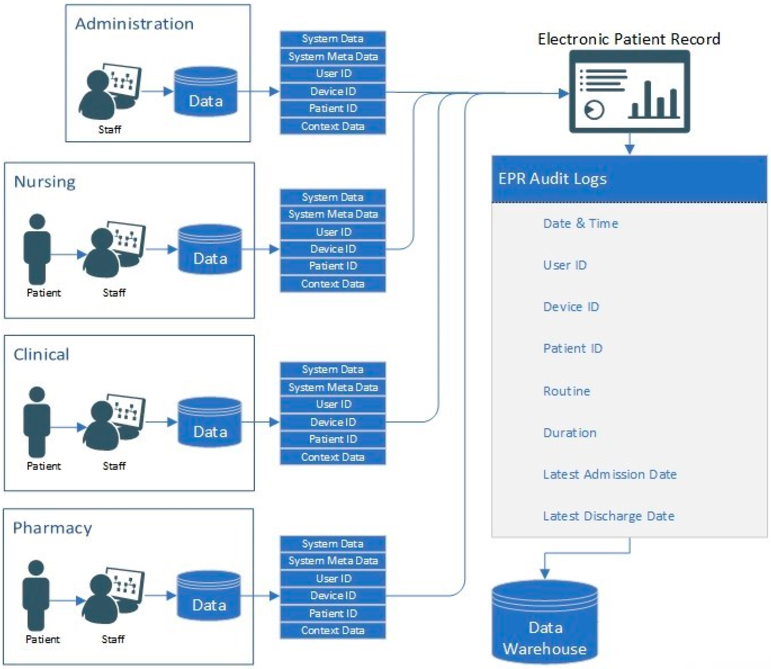
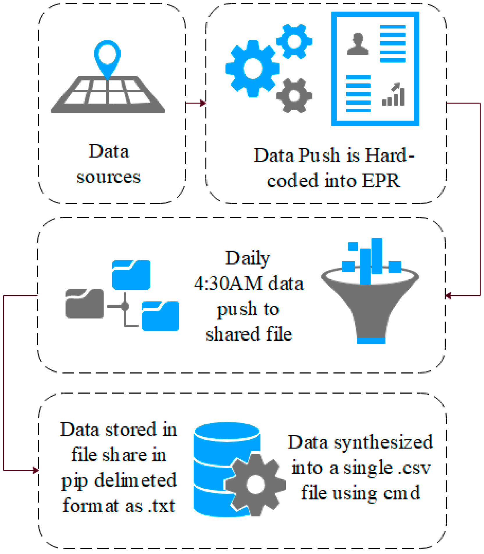
The EPR data in this study use a unique hierarchal relationship data structure (for this reason, the data cannot be queried directly and extracted). Instead, they are hard-coded into the EPR to push these data to storage on a daily basis at 04:30AM. Specifically, these data are combined into to a shared data file in pipe-delimited format (comma-delimited may cause issues with certain fields such as name, or routine). EPRs integrate many aspects of care into a single system, which are audited. Each encounter with patient data results in an audit footprint, which is stored in the data warehouse. This process is detailed in Figure 1.

These data remain in .txt format until they are synthesised into a single .csv data file using the command prompt, as presented in Figure 2. This, however, is unusual. Many EPRs (and other medical systems) use a relationship data structure; therefore, these data can instead be extracted using an SQL query and the .csv file will be created. A sample of the EPR data used in this research is presented in

Table 2. EPR audit sample data.

Time	Device	UserID	Routine *	PatientID	Duration	Admission Date	Discharged Date
00:00	362	865	PHA.ORDS	58,991	54	28/02/2016	29/02/2016
00:02	923	199	REC REC:(DRP) UK.OE	17,278	77	15/02/2016	15/02/2016
00:02	103	677	ASF	4786	13	22/07/2008	22/07/2008
00:02	103	677	ASF	4786	54	22/07/2008	22/07/2008
00:04	923	199	REC UK.OE	62,121	147	08/02/2016	08/02/2016

* The routine descriptors are outlined in Table 3. This displays only a sample of the many different routine activities that are present in the dataset.

. Each User ID, Patient ID and Device ID reading is tokenised to anonymise the data, as outlined in Algorithm 1.

Algorithm 1. Tokenisation algorithm

1.  Function: Sort (values into alphabetical order)

2.   Set: x1 a tokenised value of 1

3.  IF next value is same as previous value

4.    Assign same tokenised value

5.       ELSEIF

6. Assign a value +1 to the previous tokenisation value

7.        ELSEIF

8.    Check: All values have been tokenised

9.       Return END

10.        END

The algorithm isolates unique entries and assigns each value an incrementing number. In the dataset used in this research, there are 1515 unique User IDs, 72,878 unique Patient IDs, 2270 Device IDs and 13,722 Routine IDs. Therefore, there are 90,385 unique IDs in the dataset in total (user, patient, device and routine combined). The Routine ID is not tokenised as it denotes the tasks performed by the user on the EPR for the interaction.

The data snapshot presented in Table 1 shows, for example, that User 865 accesses the Pharmacy Orders function of the EPR on Patient 58,991 whilst using Device 362. As such, the premise of this research is to leverage the granularity of data within EPR for the development of internal-focused security application.

3.2. Framework

The methodology presented in this research involves (1) the User ID, Patient ID, Device ID and Routine data collected and pre-processed; (2) a benchmarking process to establish and define what a normal behavioural pattern is comprised of using the LOF algorithm and (3) the inclusion of a human-in-the-loop (HIL) for the investigation of identified anomalous data points. This methodology is outlined in Figure 3.

3.3. Data Pre-Processing

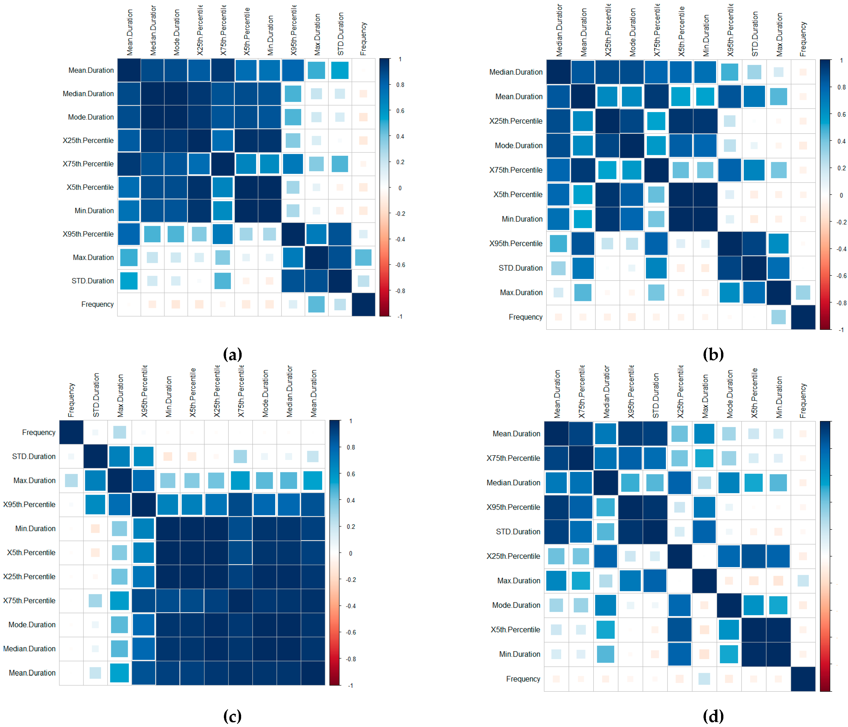
A time-series-focused statistical features extraction process is implemented in three groupings including (1) central tendency, (2) variability and (3) measures of position, calculated through the Frequency, Mean, Median, Mode, Standard Deviation, Minimum, Maximum, 1st Quartile and 3rd Quartile, the 5th Percentile and 95th Percentile features (this is further outlined in [46]). A correlation of the features for the Device ID (a), Patient ID (b), User ID (c) and Routine ID (d) is displayed in Figure 4. The correlation is implemented using the corrplot (https://cran.r-project.org/web/packages/corrplot/vignettes/corrplot-intro.html) R library package.

The visualisations display the positive and negative correlation between the features, where blue refers to positive correlation and red negative. The plots are organised using the correlation coefficient, which displays hidden structures in the matrix by means of the angular order of the eigenvectors (AOE). The ordering of the visualisation is calculated in (1) from the order of the angles (a_i), with e_i1 and e_i2 referring to the two largest eigenvalues in the correlation matrix [47].

$$a_i=\{\begin{array}{ll}\tan \left(\frac{e_{i2}}{e_{i1}}\right),& if e_{i1}>0;\\ \tan \left(\frac{e_{i2}}{e_{i1}}\right)+\pi ,& \mathit{otherwise.}\end{array}$$

(1)

On visual inspection, there are clear positive correlation patterns in each of the plots. Based on the negative correlation patterns, an omission of the frequency for the User ID, Routine and Device Interaction would be beneficial to the detection process.

In terms of the Routine and Device Interaction, the frequency patterns would relate predominately to unique routine combinations. Logically, this feature is, therefore, less significant. However, it should be retained in the Patient ID classification process.

3.4. Benchmark Profiling Using LOF

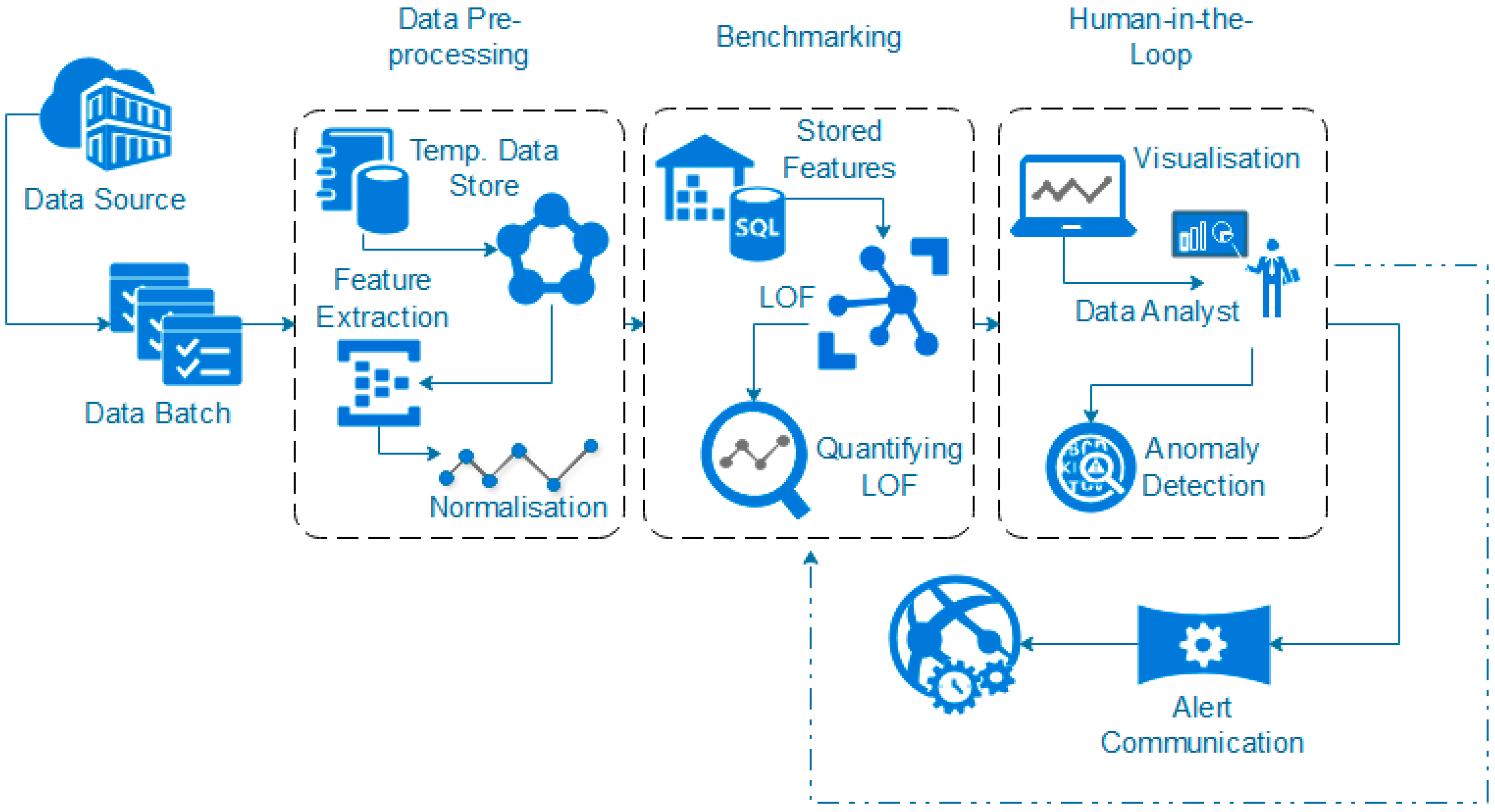
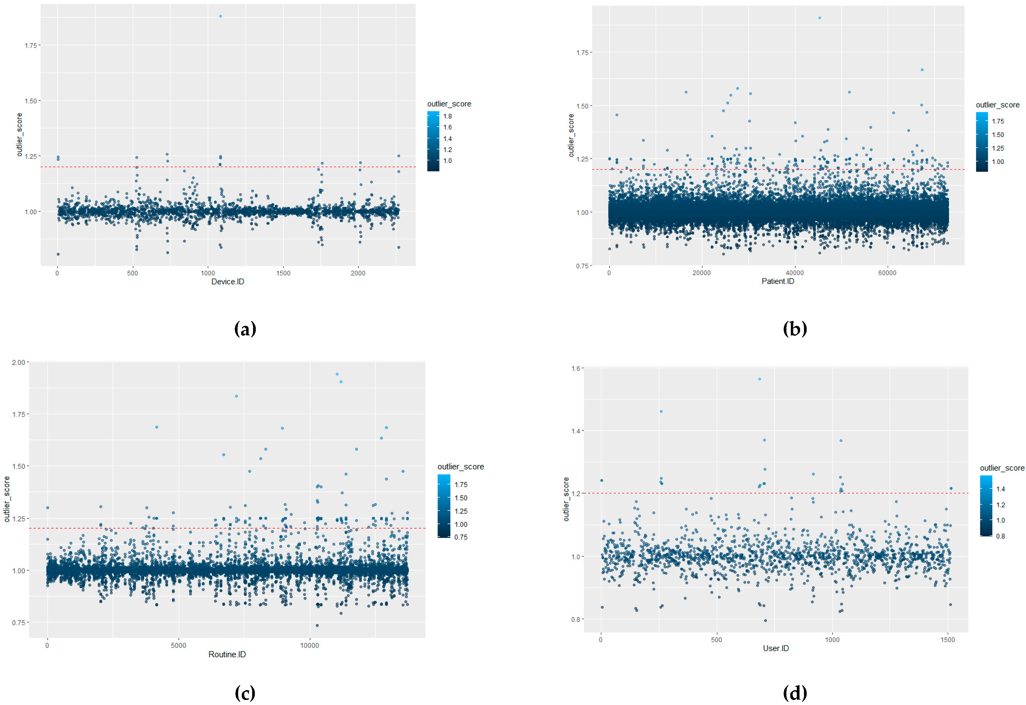
The defining of benchmark behaviours is required in order to distinguish between what is classed a normal behavioural pattern and those which should be classed as abnormal/unauthorised access. Once initial benchmarking values are set, this would tailor the system to the hospital’s unique behavioural trends. This process could, theoretically, be provided by the hospital through consultation. However, to provide a more distributable/accessible approach, it can be calculated as detailed in this section, where the initial benchmark values for each of the ID types are defined by the actual LOF approach with a HIL for confirmation.

The advantage of using LOF over other techniques is that LOF is concerned with exposing the anomalous data points. It achieves this by measuring the local deviation. In this way, data points that are a deviation from the norm are revealed [46].

In terms of EPR data, density-based outlier techniques recognise points that are deviations from related others in a single data range. This means that techniques such as LOF are beneficial for use in datasets where there might be many different professions or roles present. LOF, in particular, is advantageous over proximity-based clustering, as it considers the degree of deviance from the norm through analysing the density of one coefficient against its neighbours, whereas, if a global outlier technique is employed, a further correlation of the different hospital roles with each other would be required in order to detect irregular behaviours. The local outlier factor (LOF) calculation process involves five stages (as outlined further in [46]). Stage one concerns the k-distance computation. This is the calculation of the Euclidian distance of the k-th nearest object from p (an object). Next, the k-nearest neighbour set construction for p (Set kNN(p)) is constructed by objects within k-distance from p. Thirdly, a reachability distance computation for p is required; where the reachability distance of p to an object o in kNN(p) is defined in (2) and d(p, o) is the Euclidian distance of p to o.

$$reach-distk\left(\mathit{p},\mathit{o}\right)=max\left\{k-distance\left(\mathit{o}\right),d\left(\mathit{p},\mathit{o}\right)\right\}$$

(2)

The lrd computation for p is the local reachability density (lrd) of p, defined in (3).

$$lr{d}_k\left(\mathit{p}\right)=\frac{k}{{\Sigma }_{0\in kNN\left(\mathit{p}\right)}reach-distk\left(\mathit{p},\mathit{o}\right)}$$

(3)

The final stage is the LOF computation for p, where the local outlier factor of p is computed as displayed in (4).

$$LOF\left(\mathit{p}\right)=\frac{\frac{1}{k}{\Sigma }_{0\in kNN\left(\mathit{p}\right)}lr{d}_k\left(o\right)}{lr{d}_k\left(\mathit{p}\right)}$$

(4)

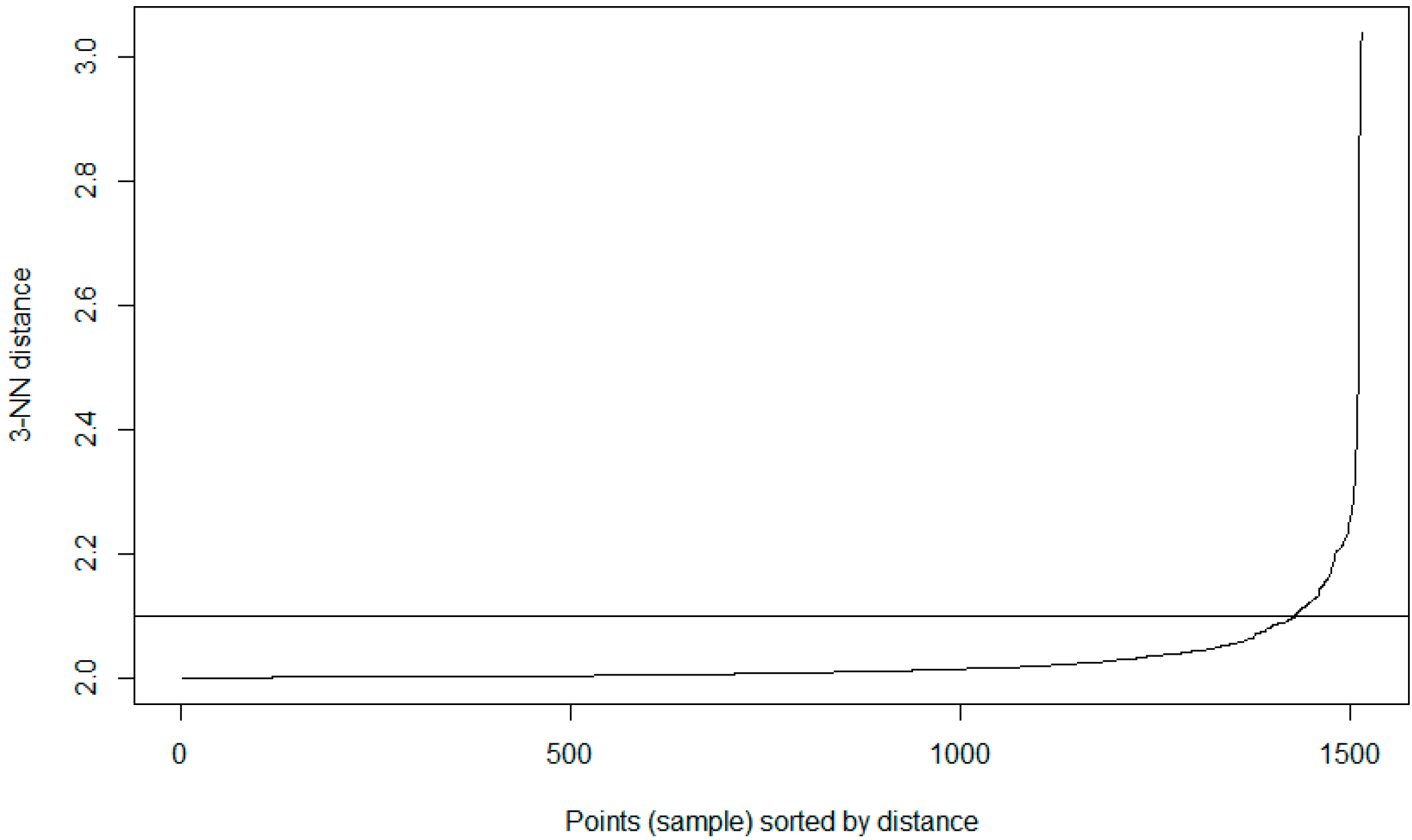
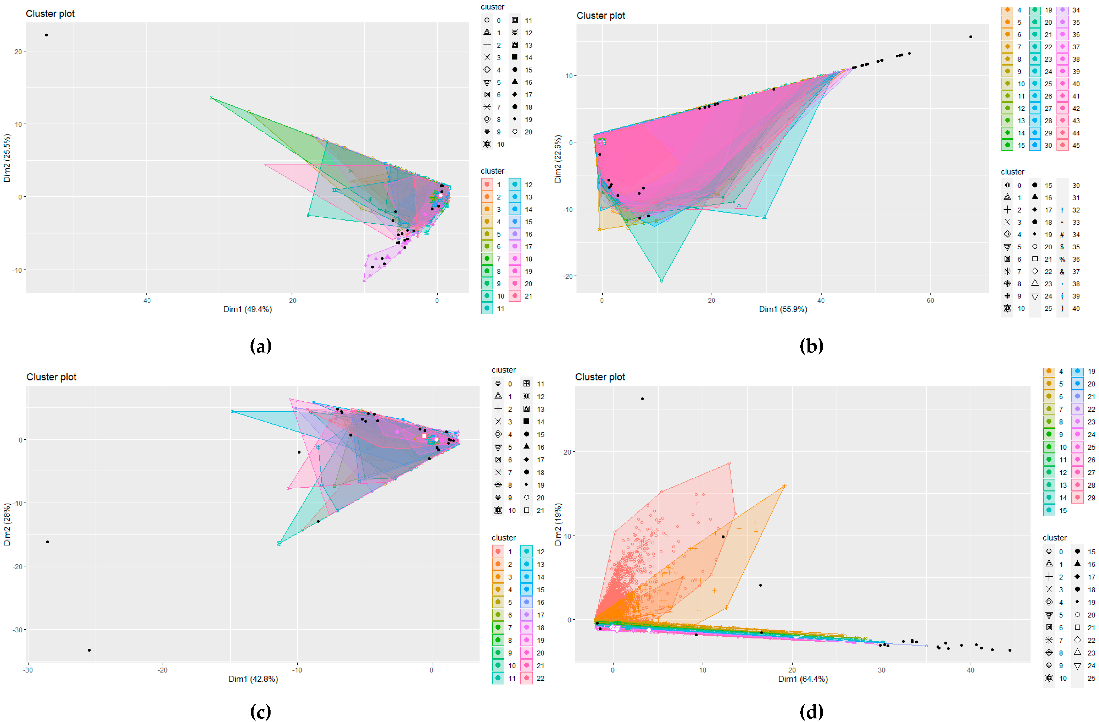
However, other solutions could be adopted, for example, DBSCAN. DBSCAN is a cluster analysis method that divides a dataset into n dimensions and forms an n-dimensional shape around each datapoint creating data clusters.

Algorithm 2. DBSCAN

1. Function: DBSCAN ()

2.    Parameters include (Data, EPS, MinPts)

3.    IF SetOfPoints is Unclassifed

4.       ClusterID = nextID(NOISE);

5.            Function: SetOfPoints.size()

6.                 FOR i from 1 to, Point = SetOfPoints(i);

7.                 IF Point is Unclassifed THEN

8                    IF ExpandCluster(SetOfPoints, Point, ClusterID, Eps, MinPts) THEN

9.                     ClusterID = nextID(ClusterID)

10.                   END FOR

11. Return DBSCAN classification

The clusters are then expanded by including other datapoints within the cluster and adding their n dimensions in the cluster. It requires two parameters: (1) ε—the minimum distance between two points to be considered neighbours and (2) MinPoints—the minimum number of points which form a dense region. Any datapoints that do not fall within a cluster can be handled as an outlier. This process is outlined in Algorithm 2, which shows a high-level DBSCAN pseudocode.

DBSCAN is often compared with LOF as an outlier model, even with large scale analysis [46]. However, DBSCAN is more applicable to cluster analysis data applications rather than anomaly detection. Clusters with varying densities cannot be easily identified, only high and low densities. Due to the lack of a weighted score, DBSCAN does not allow a patient privacy officer to prioritise their investigation into potentially inappropriate behaviour. Once the officer has investigated the noise points, there is the ‘needle-in-a-haystack’ problem of investigating border points. This is insufficient, and a weighted anomaly score is required to enable more nuanced investigation. However, a comparison of LOF with the DBSCAN approach is presented in the implementation as justification of the use of LOF for the detection methodology. As an example of active profiles within the dataset (as defined by highest frequency value) is displayed in

Table 4. User activity.

UserID	Frequency	Mean	STD	Max	5th Percentile
1016	32,557	49.50	106.66	4751	1
1320	23,674	69.57	117.32	2268	3
1025	23,104	124.06	246.66	7469	4
742	20,907	27.39	79.29	6081	2
248	19,160	125.23	264.26	8360	17

. Here, standard time frequency considerations are employed to show that User 1016 accessed data 32,557 times for a mean average of 49.50 s during the time period in which the data were collected. Further clarification on EPR data can be found in [46].

However, for clarity, User ID refers to the unique ID number assigned to the user of the EPR data. Frequency refers to the number of occurrences or actions performed by the user when accessing the EPR records. The Mean, Standard Deviation (STD), Max and 5th Percentile are time-series-based measures of central tendency and measures of dispersion used to construct the features for the LOF and DBSCAN investigation (as discussed in Section 3.3).

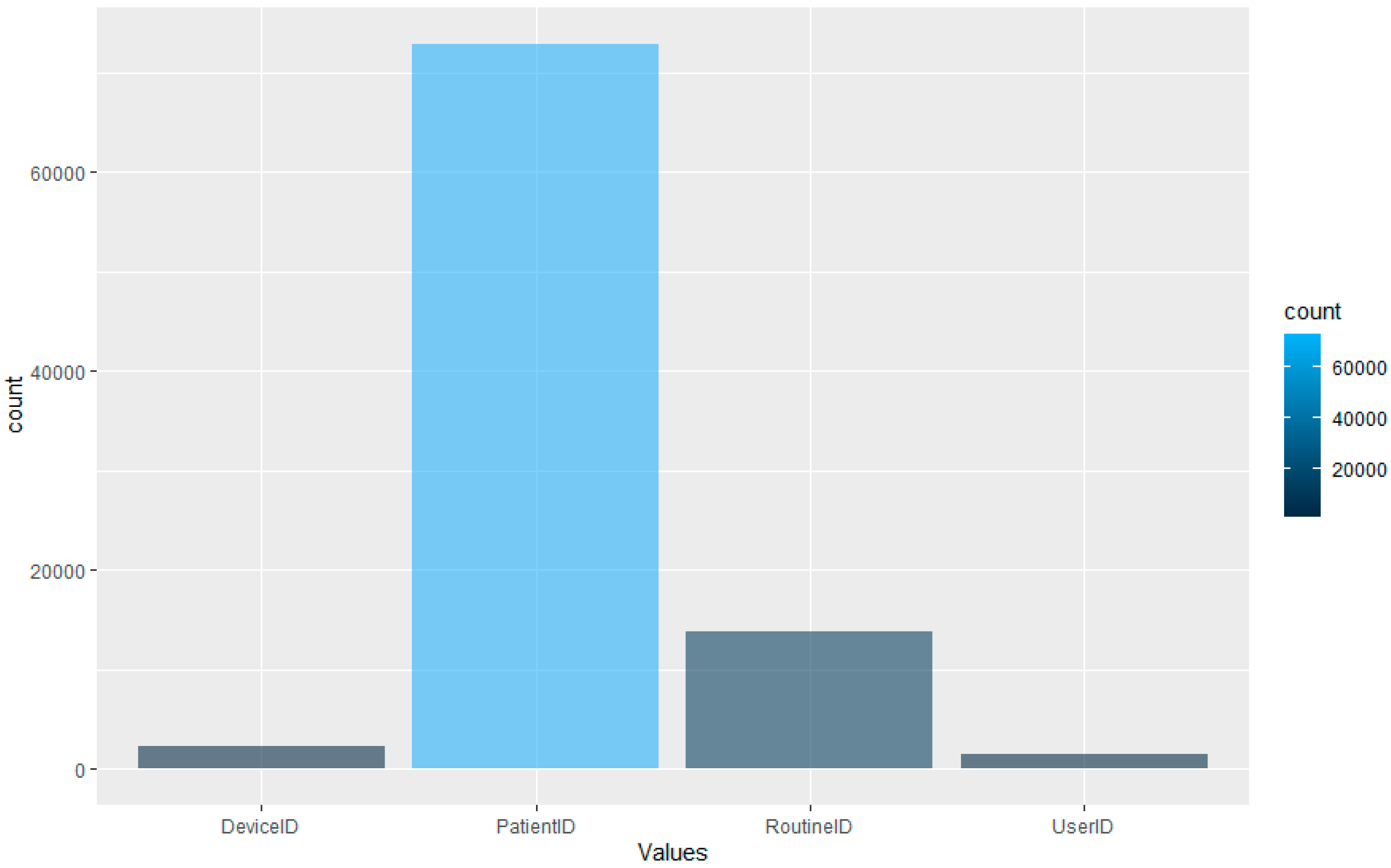
However, as the aim is to perform this type of detection using LOF. The dataset, whilst comprehensive, is unbalanced in terms of the distribution of the data across the four data types. Figure 5 displays the distribution of the data after the feature extraction and normalisation process. The graph displays that the majority of the dataset is comprised of patient ID access. This would make sense as, logically, the most likely data accessed would be related to patients within a hospital setting. The lowest portion of the dataset is comprised of the User ID information; again, this is logical, as the hospital will have fewer staff than patients.

3.5. Human-in-the-Loop

By including the HIL model, an analyst reviews the audit log anomalies and assigns a feedback score. By default, the feedback score for every anomaly is 1. The analyst can provide a feedback score in the range of 0.1 to 2. This LOF score is multiplied by the feedback score to provide the final score. Therefore, if a feedback score of 2 is given, indicating anomalous behaviour, it multiplies the anomaly score by 2 for the relevant IDs and therefore makes them more likely to be rated highly in future. If an analyst gives a score as low as 0.1, this multiplies the anomaly scores by 0.1, which effectively whitelists the IDs, making them unlikely to appear as an anomaly in future. The feedback scores are updated throughout the use of our framework by incorporating analyst feedback into the anomaly identification process. Therefore, the initial benchmark value in this experimentation is set to 1.20 based on (1) visual inspection (as displayed in Figure 5) and (2) the desire to ensure that no values close to the threshold value of 1 are selected. The choice of anomaly score is justified through consultation with the data providers, and is outlined in the following section.

4. Investigation

As previously outlined, both LOF and DBSCAN are density-based clustering approaches. DBSCAN is selected for the comparison with LOF as they both use a core and a reachability distance in order to determine outliers. However, for the DBSCAN algorithm the Optimal Value for Epsilon (EPS) must be defined. The EPS is essential for determining when two points are considered neighbours. Using a KNN distance plot, presented in Figure 6, the optimal/threshold EPS is identified as 2.1 and defined by the horizontal ab-line overlaid onto a plot of the sample points against the 3-NN distance.

4.1. DBSCAN Outlier Detection Results

The DBSCAN calculation process is implemented using the dbscan (https://cran.r-project.org/web/packages/dbscan/index.html) R package.

Table 5. Density-Based Spatial Clustering of Applications with Noise (DBSCAN) output.

User ID	User ID Type	Patient ID	Patient ID Type	Device ID Row_Id	Device ID Type	Routine ID Row_Id	Routine ID Type
119	noise	803	noise	1	noise	MPI ZCUS.UK.SCH ZCUS.UK.LETTER	noise
126	noise	804	noise	2	noise	ZCUS.UK.LETTER VH SPC OE	noise
144	noise	805	noise	3	noise	ASF	core
203	noise	806	noise	4	noise	ASF MPI	core
226	noise	807	noise	5	noise	ASF NOTE ZCUS.UK.LETTER	core

presents a sample of five rows of the DBSCAN results for User ID, Patient ID, Device ID and Routine ID. DBSCAN does not apply a weighted score to the results, and therefore the results are classified as one of three point types. A core point is classified as a point that belongs to a cluster. A boundary point is within the epsilon of a core point but does not meet the criteria of min_points to be considered a core point. Finally, noise points are not assigned to any cluster. A visualisation of the DBSCAN output is implemented in Figure 7 using the factoextra (https://cran.r-project.org/web/packages/factoextra/index.html) R library package, which show cluster plots of the predictions. The cluster against the noise identification is outlined in Table 5.

In Table 5, the User ID is displayed, which is the identification code of the user accessing the data record, the patient record being accessed (Patient ID), the device being used (Device ID) and the action (Routine ID) being conducted. The data displayed in Table 5 outline which point type (as previously outlined) the classifier predicts the data point as belonging to for its corresponding class. For example, the first row shows that DBSCAN considers that User 119 does not belong to a cluster and classes the data point as noise. The data point for Patient ID 803 is also considered noise, as is Device ID 1. As previously demonstrated in Table 2 and

Table 3. Routine descriptors.

Routine	Descriptor
PHA.ORDS	Pharmacy Orders
REC REC:(DRP) UK.OE	Recent Clinical Results Recent Clinical Results:(Departmental Reports) UK.View Orders
ASF	Assessment Forms
REC UK.OE	Recent Clinical Results UK.View Orders

, the routine action is abbreviated. These tasks are often unique to the infrastructure, so defining the full list is not possible within the constraints of this paper. However, some actions, such as assessment forms (ASF), are common actions. In this case, the ASF routine has been classed as a core data point. The results achieved are visualised in Figure 7.

The clusters are identifiable by the coloured areas, with the black dots classed as outliers or anomalous points. The visualised results are summarised in

Table 6. DBSCAN Output.

Class	Objects	Clusters	Noise
DeviceID	2270	21	21
PatientID	72,878	45	35
UserID	1515	22	23
RoutineID	13,722	29	23

. The table displays the number of objects (data points) for each class, the number of assumed clusters and the number of noise points. The total number of anomalies is calculated by adding the noise total.

As the results show, due to the lack of a weighted score, DBSCAN does not allow a patient privacy officer to prioritise their investigation into potentially inappropriate behaviour. Once the officer has investigated the noise points, there is the ‘needle-in-a-haystack’ problem of investigating border points relating to it. As such, the anomaly total provided is misleading and may be considerably higher if the related border points are also anomalous. A weighted anomaly score would offer a solution as mitigation for this challenge and enable more nuanced investigation.

4.2. LOF Outlier Detection Results

The LOF visualisation in Figure 8 creates an anomaly priority ordering display, where the advantage of a weighted anomaly score is apparent. Each of the classes are displayed in four separate plots, (a) to (e). The data points are plotted with the ID on the x-axis and the anomaly score on the y-axis. This means that the points can be integrated into an interactive list (using for example the R plotly (https://cran.r-project.org/web/packages/plotly/index.html) package), where the datapoints display the ID number. The data point colour is defined by the anomaly score. Where points with a higher anomaly score are coloured with a lighter blue. This enables an analyst to investigate the associated activity with the ID. By visualizing the LOF results in this manner, activities such as staff members misusing their access privileges can be investigated, whilst the HIL approach facilitates a refining of the system for increased situational awareness.

Using the feature vectors, the LOF process is implemented using the outliers (https://cran.r-project.org/web/packages/outliers/index.html) R library package. A LOF score of 1.0 or below indicates a dense region and is classed as being comparable to its neighbours, i.e., an inlier [46]. A value significantly above 1 therefore indicates an outlier (anomaly). The use of visual inspection for the benchmark would be considered a HIL approach. HIL approaches are common approaches used for decision-based modelling [48,49]. This would only be required for the first stage and could, in future, be automated.

4.3. Outlier Validation

As validation for the benchmark process, (beyond the use of visual inspection), an overview of the data patterns is provided. The consideration would be to investigate how the LOF anomaly/normal patterns relate to in a real-world setting as justification for the anomaly scores. Using this above approach, 358 anomalies out of 90,385 unique IDs are presented. The threshold value would require further refinement using the HIL approach to reduce level of anomalies for a more accurate identification process. However, it is clear that this approach is capable of detection anomalies, but the HIL is crucial for labelling and refining the detection methodology. The visualisation provided by LOF offers a grading-based score for the anomaly detection process, and future work could exploit this by facilitating a grading system. For example, values over 2 could be treated with a higher priority than those closer to 1.2. Furthermore, with regard to achieving false negative results (anomalies labelled as normal, but are in-fact abnormal), the risk would be minimal. In order to be classed as normal, but be anomalous, the data access/device usage pattern would have to conform to the expected guidelines outlined above, which is a benchmark behaviour unique to the hospital setting.

4.4. Discussion

In this paper, two density-based classification techniques (DBSCAN and LOF) were employed for the detection of anomalies within EPR data. The techniques are selected with the consideration of factoring in a HIL approach. For that reason, a consideration of the visualisation of the results is also essential for providing legitimate information to the user. For the DBSCAN, the EPS was identified as 2.1 and the experimentation was subsequently conducted under this consideration. Based on the experimentation results, the recommendation is to adopt LOF for the process, due to the use of the weighted score. The addition of the weighted score also has clear benefits for the visualisation of the results, as demonstrated through the clarity of the plots presented in Figure 8, compared with those in Figure 7.

Furthermore, as validation of the outliers detected, under consultation with the hospital providing the data, the following offers a justification for the benchmark value of 1.2 and clarification of what would be classed as normal/abnormal behaviour within the infrastructure.

• With regard to the User ID, a user typically spends 300 s (5 min) or less performing an action on a patient. This pattern is reflected in the dataset, where the most active users rarely exceed 400 s. This would relate to the LOF score of 1. However, anomalies, such as 7000 s (almost 2 h), are recorded in the dataset, with user 685 standing out as an anomaly. These values will be recorded as outliers in the LOF process.
• In terms of the Patient ID, the dataset patterns are typically clustered around 1000-s-access patterns (17 min); however, with some notable anomalies, such as the user that accesses a patient ID for 3750 s and some even over 5000 s. As confirmed by the hospital, 1000 s is a typical time block for a patient record to be accessed and would be the LOF score of 1. Most clinic sessions last 15 min, which would confirm this observation. However, unlike with User IDs, there are no clear observations that patient IDs are accessed for longer on different devices than others.
• As confirmed under consultation with the hospital, Device ID access is typically around 400 s, with some users accessing a device for no longer than a few seconds. However, one user does perform a routine on a device for over 1600 s. Additionally, 300 s (5 min) or less is typically spent on a device performing an action on a patient. Similar observations, with varying datapoints, show that it is atypical for a device to be used for longer than approximately 600 s. Some exceptions, such as the data that are accessed for 1700 s. Therefore, 400 s is the initial benchmark for accessing devices in the dataset and would likely produce an LOF score of 1.
• Routine ID demonstrates that 400 s is the typical time spent on a device in the dataset, with some exceptions, such as the routine that is accessed for 1700 s. Due to the routines having extreme anomalies within the dataset (such as 12,000 s), the scale makes observations more challenging to determine for Routine ID. A routine appears to be typically performed in under 1000 s on a patient. Therefore, 1000 s is the initial benchmark for typical routine behaviour in the dataset.

5. Conclusions

The research presented in this paper offers a significant contribution in patient privacy monitoring. Proactive monitoring of audit logs is required to achieve comprehensive situational awareness of activity within an EPR. The system framework uses the LOF algorithm to detect unusual data patterns, labelling points as normal or anomalous, under the consideration of a HIL approach. Current procedure-based models are insufficient for internal anomaly detection. Reputational damage to the hospital is caused by the fact that most information security incidents are detected by the patient, or staff member, whose privacy has been violated rather than by a security analyst. Therefore, this work represents research towards a system to ensure the confidentiality and privacy of EPR systems. As such, this research project will increase the situational awareness of data flow and actively address the issue of data misuse. Machine learning algorithms have the capability to observe and learn patterns of data and profile users’ behaviour, which can then be represented visually. Therefore, our future work will look towards the integration of machine learning. Specifically, we will assess the performance of our approach against machine learning-based techniques, for example, against a Support Vector Machine (SVM) and decision tree. This will ensure the safeguarding of patient privacy in healthcare systems.