Climate Sensitive Tree Growth Functions and the Role of Transformations

Abstract
1. Introduction
2. Materials and Methods
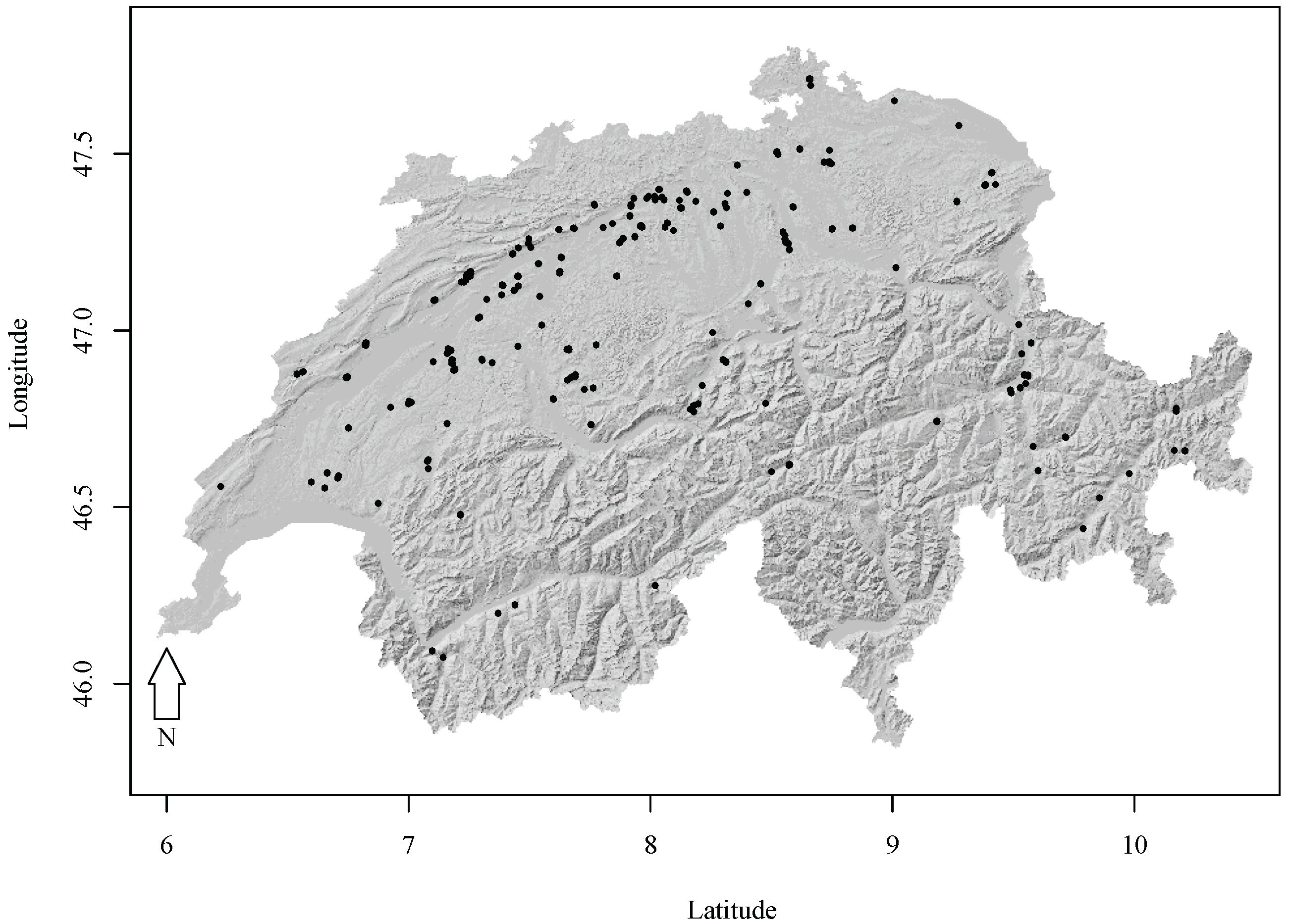
2.1. Experimental Forest Research Data
2.2. Explanatory Variables
2.2.1. Competition
2.2.2. Stand Development
2.2.3. Site
2.2.4. Stand Density
2.2.5. Thinning
2.2.6. Mixture
2.2.7. Climate
2.2.8. Years Past 1940
2.3. Model Fitting
2.3.1. Base Model
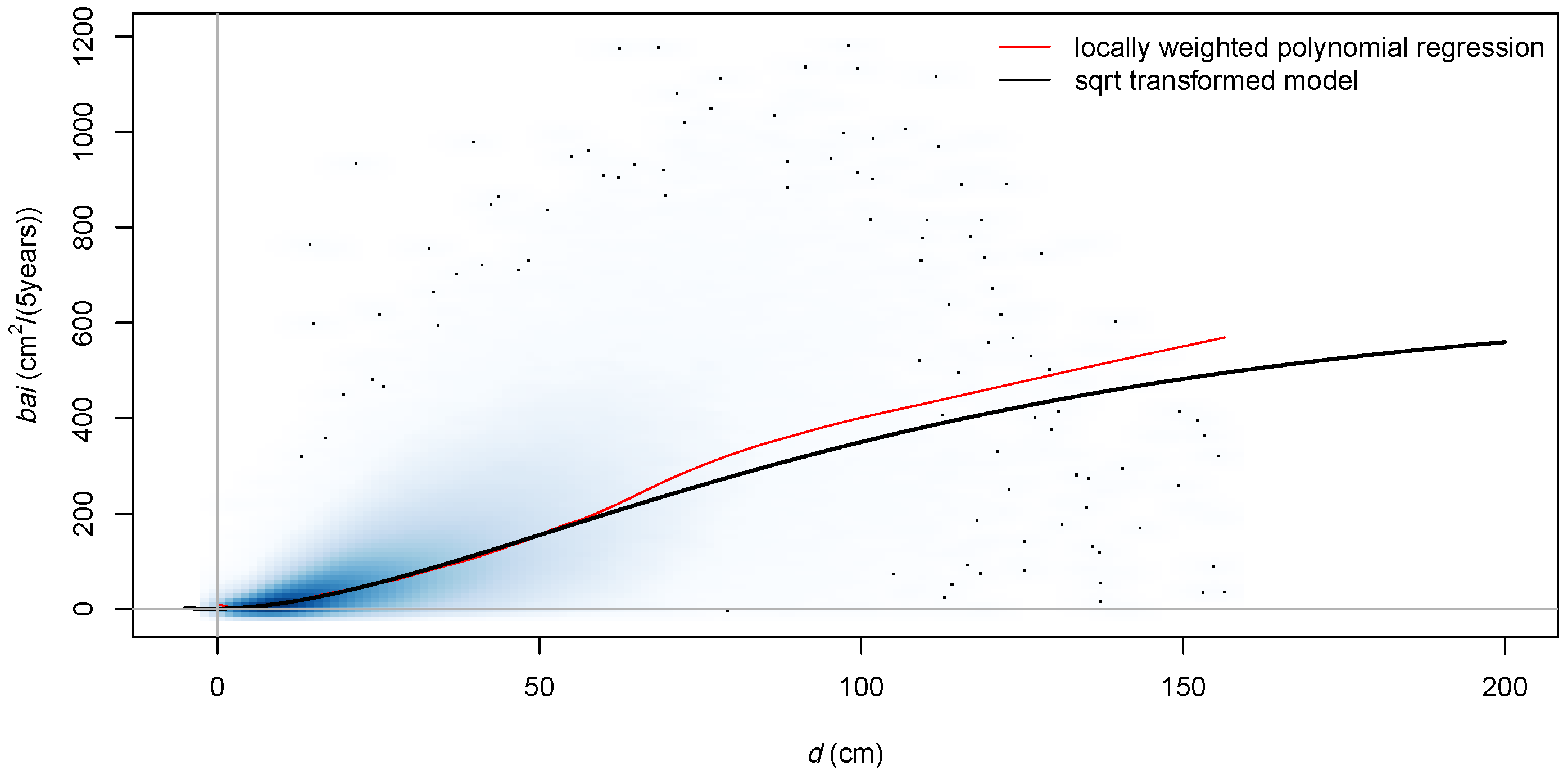
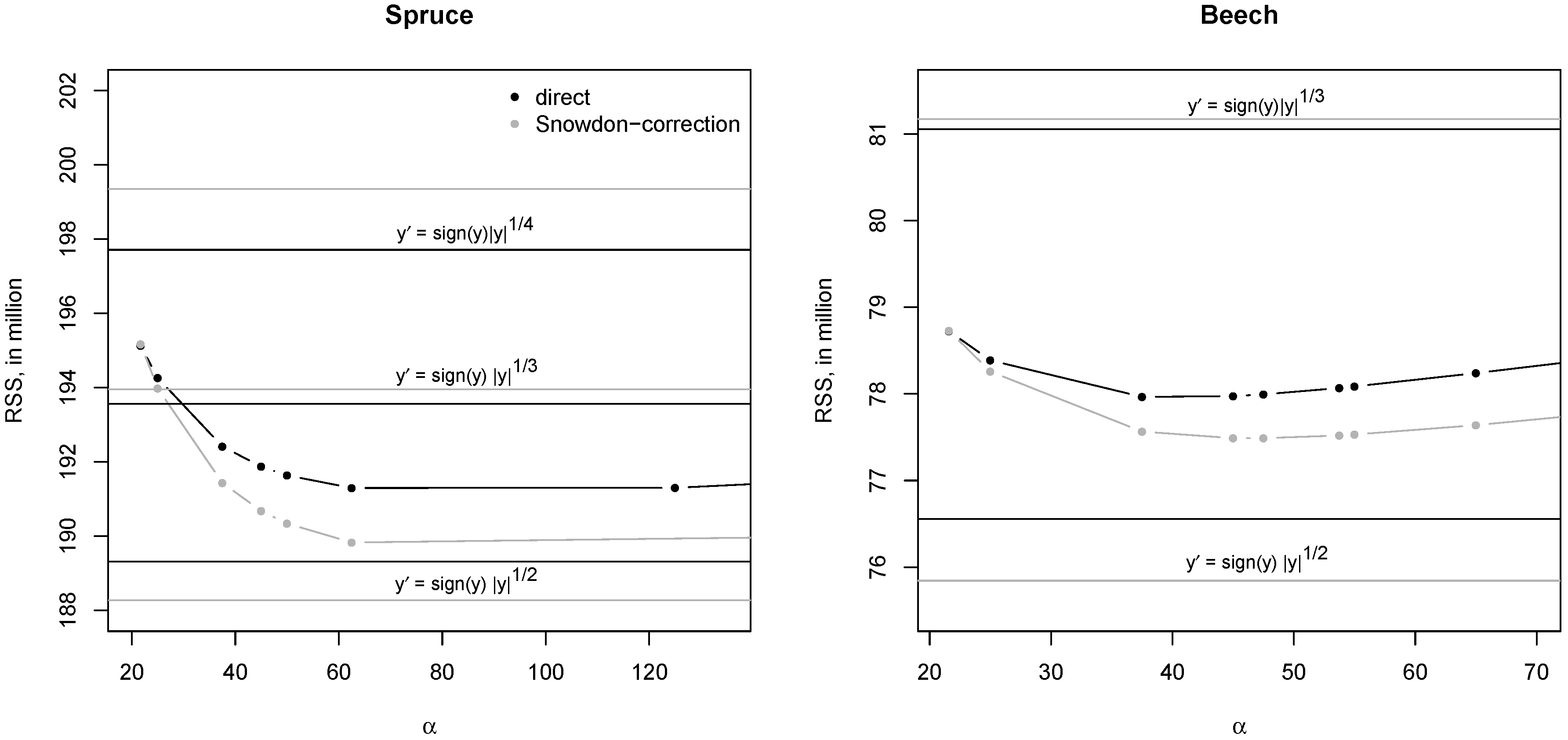
2.3.2. Transformation
- = sign(y) , with
- , with
2.3.3. Model Selection
2.3.4. Model Validation
3. Results
3.1. Role of Transformation
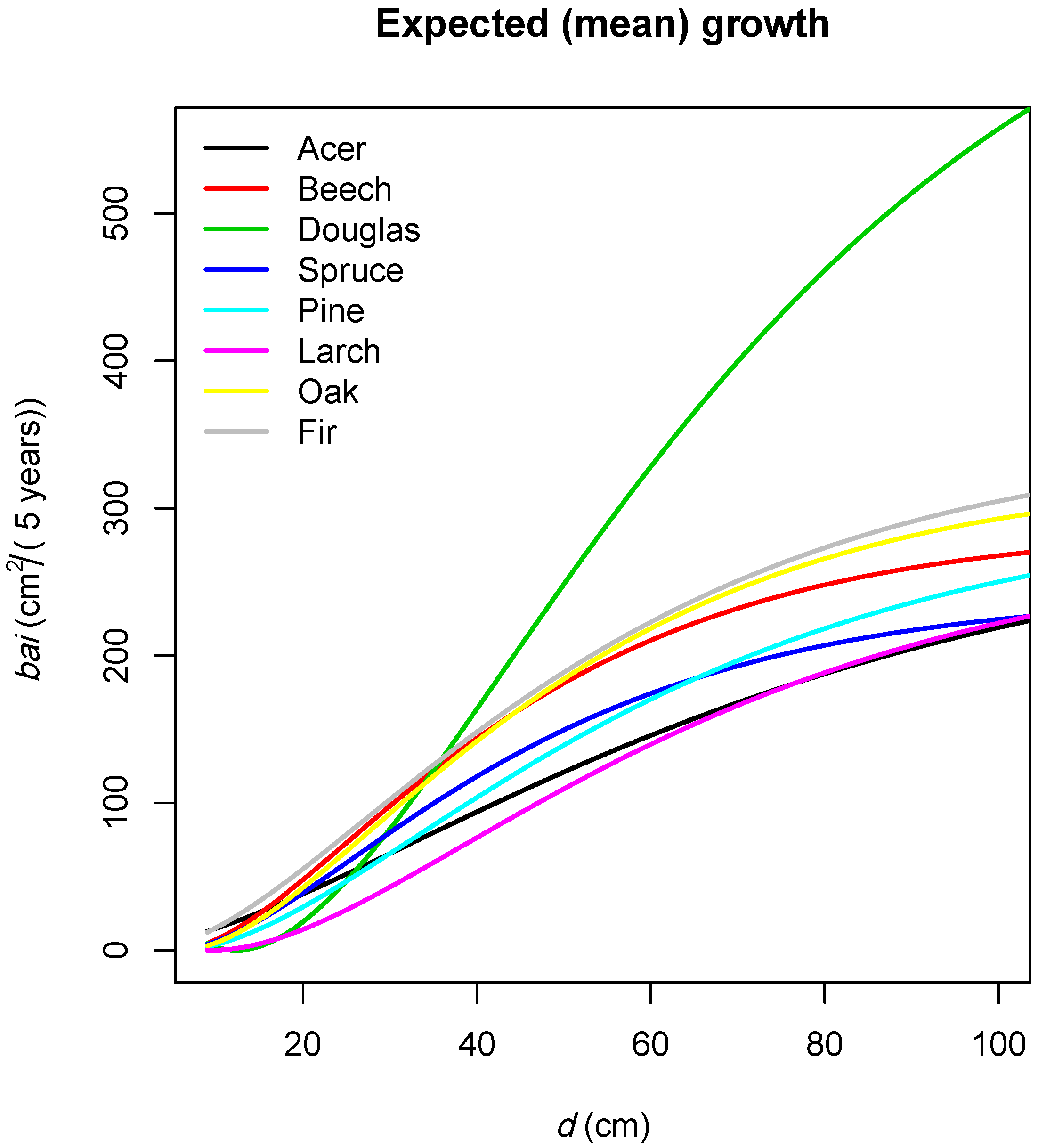
3.2. Climate Sensitive Growth Functions
3.2.1. Overview
3.2.2. Effects
Competition
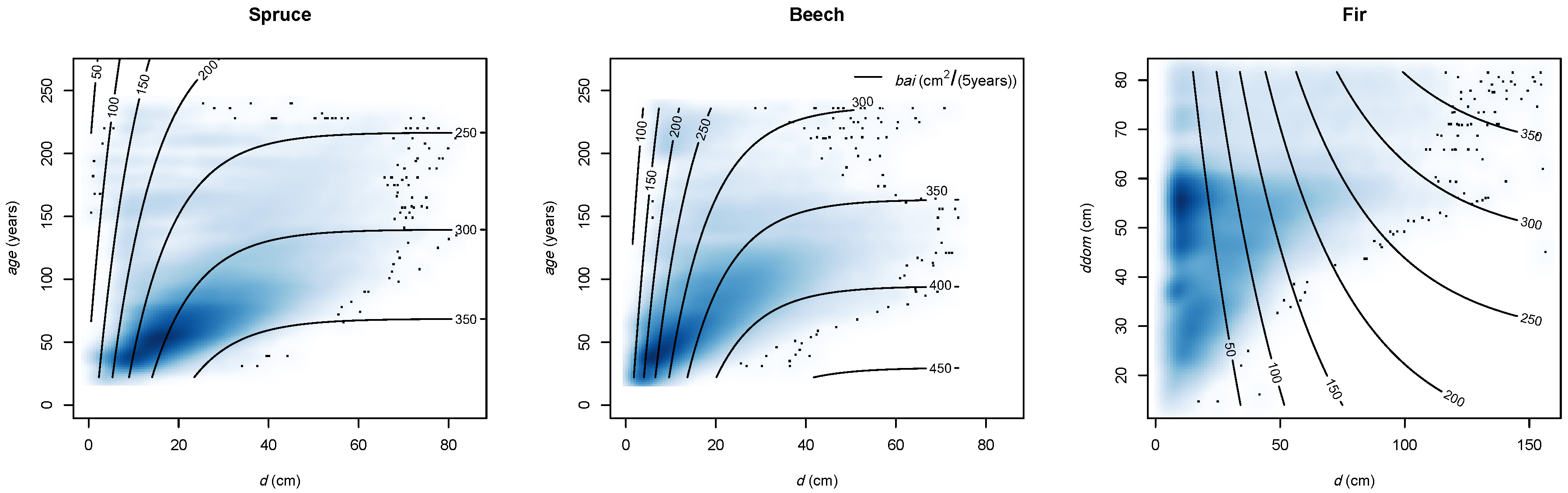
Stand Development
Site
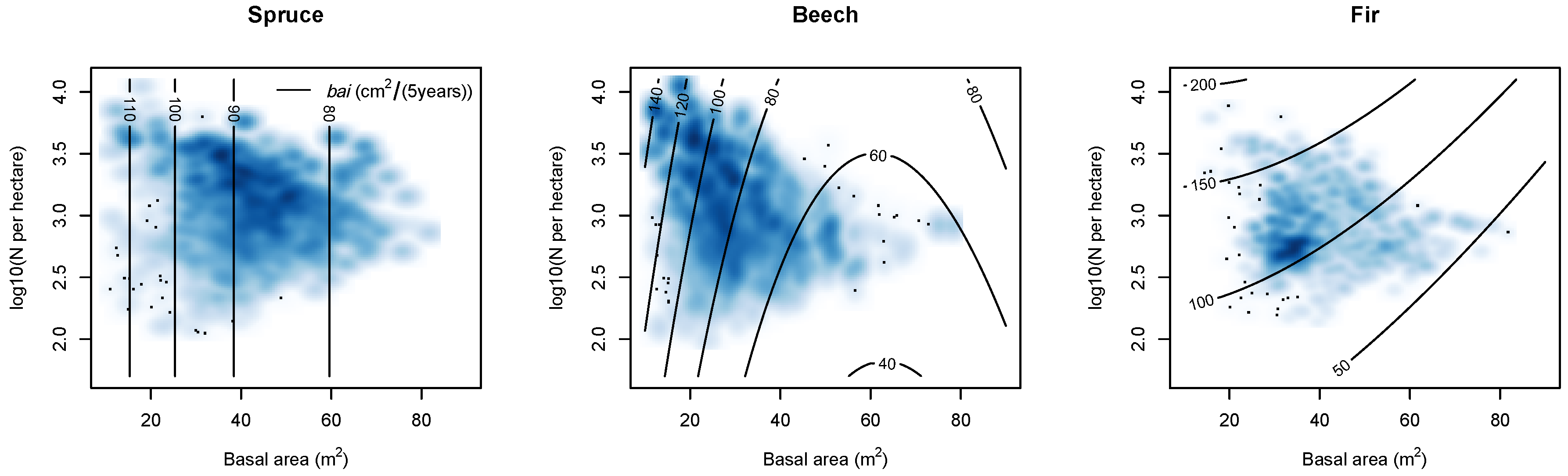
Stand Density
Thinning
Mixture
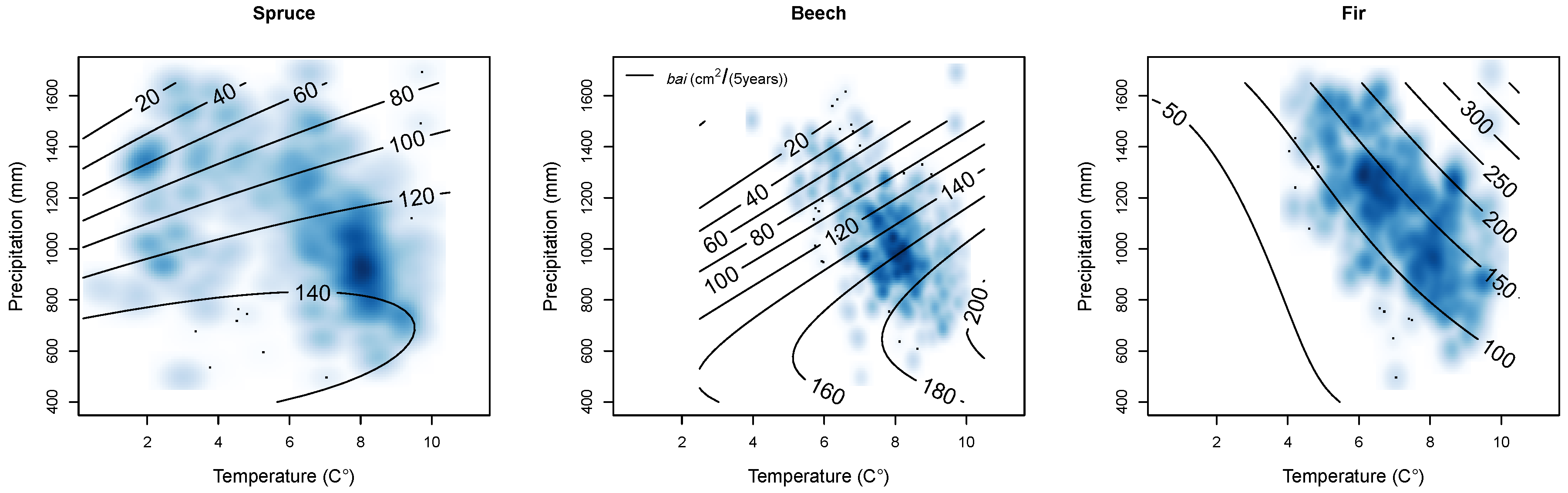
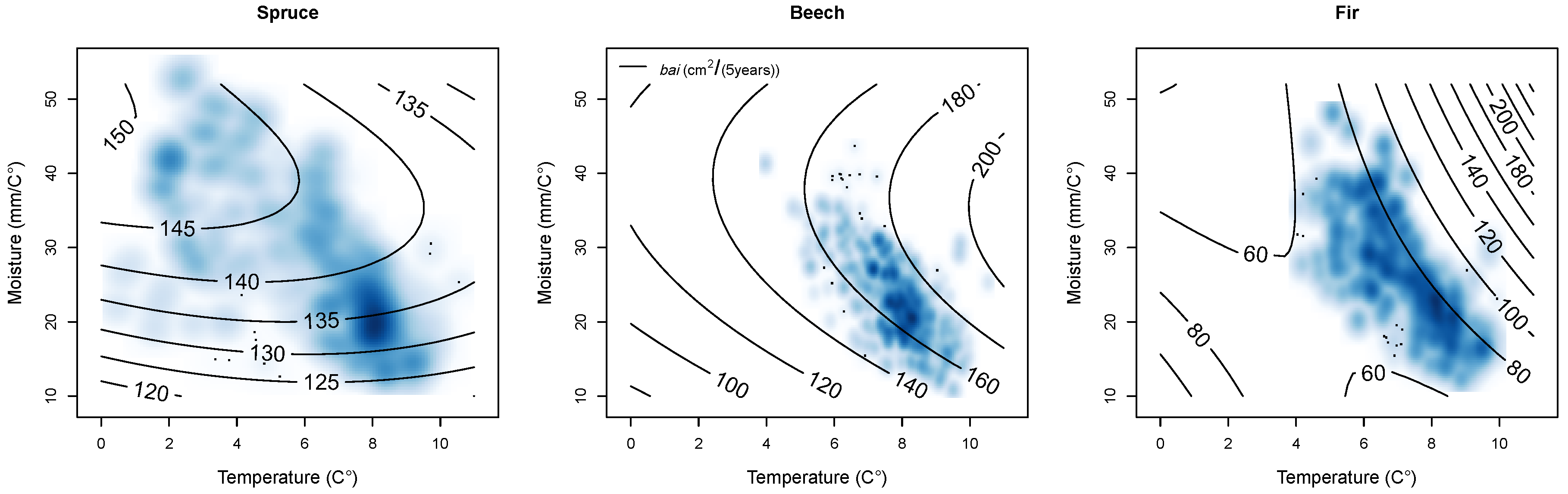
Climate
Non Significant Effects
4. Discussion
4.1. Transformation
4.2. Estimation Method
4.3. Estimated Effects
4.3.1. Explained Variance
4.3.2. Model Selection
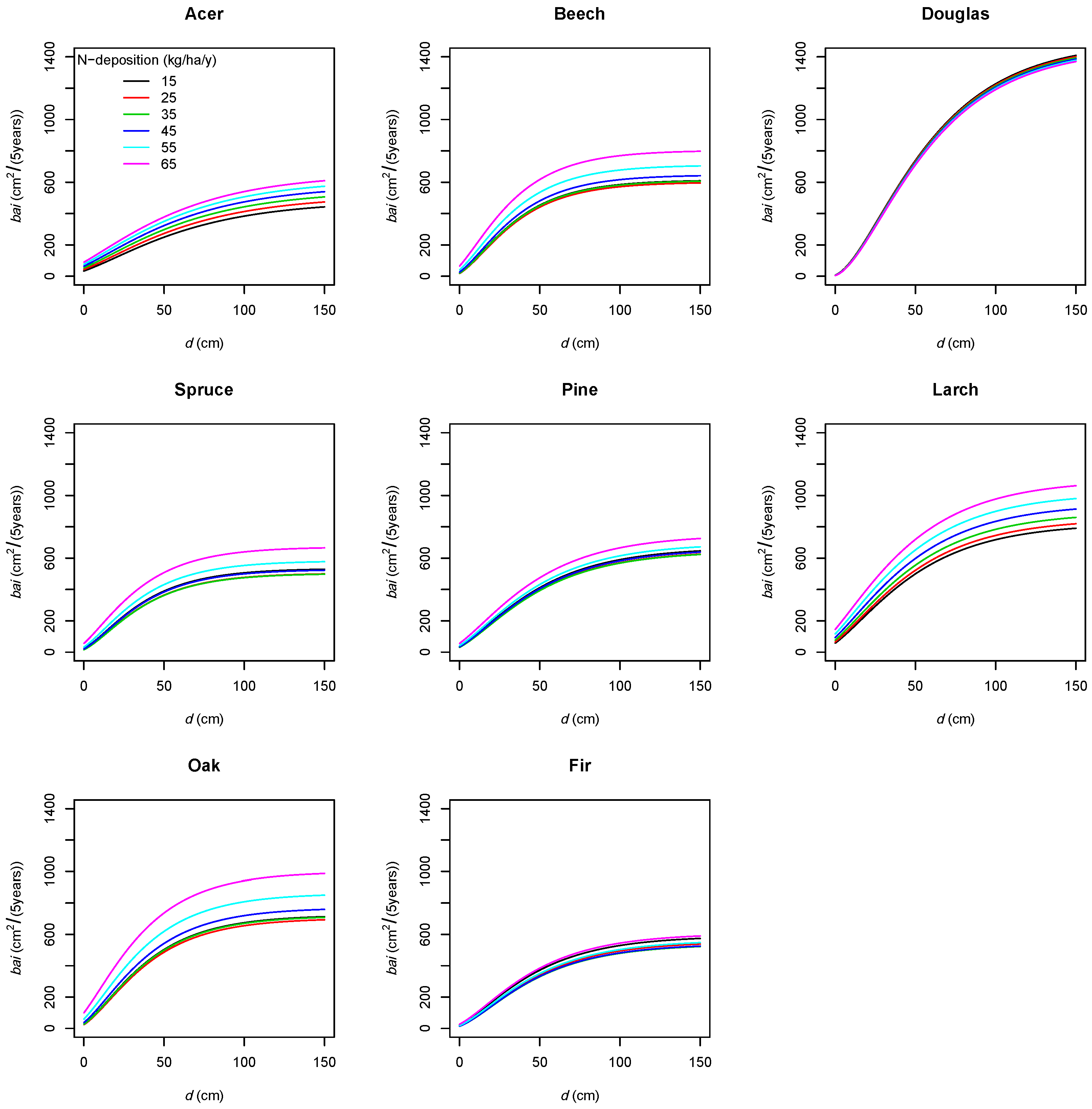
4.3.3. Nitrogen
4.3.4. Years Past 1940
5. Conclusions
Supplementary Materials
Acknowledgments
Conflicts of Interest
Abbreviations
| d | (single tree-specfic) tree diameter (at 1.3 m height, breast height) in cm |
| dominant diameter in cm: quadratic mean of the 100 thickest trees per hectare | |
| A | total plot area in hectares (104 m2) |
| a | stand age in years |
| tree basal area (at breast height) in m2: | |
| total plot basal area in m2/ha: | |
| ith year of the measurement | |
| basal area increment normalized to 5-year period: | |
| relative basal area increment: | |
| cumulative basal area: | |
| basal area of larger trees: | |
| relative basal area of larger trees: | |
| percentage of basal area previously harvested in relation to | |
| total number of trees per hectare in a plot | |
| percentage of stems harvested since last inventory | |
| crown surface area in m2: with the imputed crown radius, the imputed crown length | |
| crown base (height where the living crown starts), in m | |
| crown cross sectional area in m2 | |
| stand density index: | |
| crown competition index Equation (2) | |
| change in crown competition index after harvesting has taken place Equation (2) | |
| leading tree species is coniferous (holding maximum basal area in a stand) | |
| if the observation year is before 1940, it is zero, otherwise the current year of observation−1940. | |
| p | yearly mean precipitation sum over period length in mm. Calculated for physiological year, meaning that the sum was taken from October until September, in contrast to calender years [42]. |
| t | mean physiological year temperature, over intervals such as p. |
| m | Aridity index (defined by deMartonne ([38], [p. 520])). . Since this index means smaller values have higher aridity, its inverse interpretation is more intuitive. Consequently it was labeled “moisture-index” (m). In contrast to precipitation and temperature, moisture shows higher explanatory power in the spring months [42]; hence only the spring months (March–June) over periods were used to calculate the moisture index. |
References
- Bolte, A.; Ammer, C.; Löf, M.; Madsen, P.; Nabuurs, G.J.; Schall, P.; Spathelf, P.; Rock, J. Adaptive forest management in central Europe: Climate change impacts, strategies and integrative concept. Scand. J. For. Res. 2009, 24, 473–482. [Google Scholar] [CrossRef]
- Lindner, M.; Fitzgerald, J.B.; Zimmermann, N.E.; Reyer, C.; Delzon, S.; van der Maaten, E.; Schelhaas, M.J.; Lasch, P.; Eggers, J.; van der Maaten-Theunissen, M.; et al. Climate change and European forests: What do we know, what are the uncertainties, and what are the implications for forest management? J. Environ. Manag. 2014, 146, 69–83. [Google Scholar] [CrossRef] [PubMed]
- Wykoff, W.R. A Basal Area Increment Model for Individual Conifers in the Northern Rocky Mountains. For. Sci. 1990, 36, 1077–1104. [Google Scholar]
- Monserud, R.A.; Sterba, H. A basal area increment model for individual trees growing in even- and uneven-aged forest stands in Austria. For. Ecol. Manag. 1996, 80, 57–80. [Google Scholar] [CrossRef]
- Pretzsch, H.; Biber, P.; Dursky, J. The single tree-based stand simulator SILVA-construction, application and evaluation. For. Ecol. Manag. 2002, 162, 3–21. [Google Scholar] [CrossRef]
- Nagel, J.; Albert, M.; Schmidt, M. Das waldbauliche Prognose- und Entscheidungsmodell BWINPro 6.1: Neuparametrisierung und Modellerweiterungen. Wald Holz 2002, 57, 486–492. [Google Scholar]
- Zell, J. A Climate Sensitive Single Tree Stand Simulator for Switzerland; Technical Report; Swiss Federal Institute of Forest, Snow and Landscape Research, WSL: Birmensdorf, Switzerland, 2016. [Google Scholar]
- Reynolds, K.M.; Twery, M.; Lexer, M.J.; Vacik, H.; Ray, D.; Shao, G.; Borges, J.G. Decision Support Systems in Forest Management. In Handbook on Decision Support Systems 2; Springer: Berlin/Heidelberg, Germany, 2008; pp. 499–533. [Google Scholar]
- Oberhuber, W.; Kofler, W. Topographic influences on radial growth of Scots pine (Pinus sylvestris L.) at small spatial scales. Plant Ecol. 2000, 146, 229–238. [Google Scholar] [CrossRef]
- Lévesque, M.; Walthert, L.; Weber, P. Soil nutrients influence growth response of temperate tree species to drought. J. Ecol. 2016, 104, 377–387. [Google Scholar] [CrossRef]
- Fritts, H.C. Tree Rings and Climate; Academic Press: Cambridge, MA, USA, 1976; p. 567. [Google Scholar]
- Biging, G.S.; Dobbertin, M. Evaluation of Competition Indices in Individual Tree Growth Models. For. Sci. 1995, 41, 360–377. [Google Scholar]
- Laubhann, D.; Sterba, H.; Reinds, G.J.; De Vries, W. The impact of atmospheric deposition and climate on forest growth in European monitoring plots: An individual tree growth model. For. Ecol. Manag. 2009, 258, 1751–1761. [Google Scholar] [CrossRef]
- Andreassen, K.; Tomter, S.M. Basal area growth models for individual trees of Norway spruce, Scots pine, birch and other broadleaves in Norway. For. Ecol. Manag. 2003, 180, 11–24. [Google Scholar] [CrossRef]
- Belcher, D.M.; Holdaway, M.R.; Brand, G.J. A Description of STEMS—The Stand and Tree Evaluation and Modeling System; General Technical Report NC-79; U.S. Dept. of Agriculture, Forest Service, North Central Forest Experiment Station: St. Paul, MN, USA, 1982; p. 79.
- Schelhaas, M.J.; Hengeveld, G.M.; Heidema, N.; Thürig, E.; Rohner, B.; Vacchiano, G.; Vayreda, J.; Redmond, J.; Socha, J.; Fridman, J.; et al. Species-specific, pan-European diameter increment models based on data of 2.3 million trees. For. Ecosyst. 2018, 5, 21. [Google Scholar] [CrossRef]
- Rohner, B.; Waldner, P.; Lischke, H.; Ferretti, M.; Thürig, E. Predicting individual-tree growth of central European tree species as a function of site, stand, management, nutrient, and climate effects. Eur. J. For. Res. 2017, 1–16. [Google Scholar] [CrossRef]
- Nothdurft, A.; Wolf, T.; Ringeler, A.; Böhner, J.; Saborowski, J. Spatio-temporal prediction of site index based on forest inventories and climate change scenarios. For. Ecol. Manag. 2012, 279, 97–111. [Google Scholar] [CrossRef]
- Albert, M.; Schmidt, M. Climate-sensitive modelling of site-productivity relationships for Norway spruce (Picea abies (L.) Karst.) and common beech (Fagus sylvatica L.). For. Ecol. Manag. 2010, 259, 739–749. [Google Scholar] [CrossRef]
- Bugmann, H. A Review of Forest Gap Models. Clim. Chang. 2001, 51, 259–305. [Google Scholar] [CrossRef]
- Reyer, C.; Lasch-Born, P.; Suckow, F.; Gutsch, M.; Murawski, A.; Pilz, T. Projections of regional changes in forest net primary productivity for different tree species in Europe driven by climate change and carbon dioxide. Ann. For. Sci. 2014, 71, 211–225. [Google Scholar] [CrossRef]
- Iverson, L.R.; Prasad, A.M. Potential Changes in Tree Species Richness and Forest Community Types following Climate Change. Ecosystems 2001, 4, 186–199. [Google Scholar] [CrossRef]
- Trasobares, A.; Zingg, A.; Walthert, L.; Bigler, C. A climate-sensitive empirical growth and yield model for forest management planning of even-aged beech stands. Eur. J. For. Res. 2016, 135, 263–282. [Google Scholar] [CrossRef]
- Zingg, A. Diameter and Basal Area Increment in Permanent Growth and Yield Plots in Switzerland. In Growth Trends in European Forests; Springer: Berlin/Heidelberg, Germany, 1996; pp. 239–265. [Google Scholar]
- West, P.W. Use of diameter increment and basal area increment in tree growth studies. Can. J. For. Res. 1980, 10, 71–77. [Google Scholar] [CrossRef]
- Assmann, E.; Davis, P.W. The Principles of Forest Yield Study: Studies in the Organic Production, Structure, Increment and Yield of Forest Stands; Elsevier Science: New York, NY, USA, 1970; p. 521. [Google Scholar]
- Lhotka, J.M. Examining growth relationships in Quercus stands: An application of individual-tree models developed from long-term thinning experiments. For. Ecol. Manag. 2017, 385, 65–77. [Google Scholar] [CrossRef]
- Hansen, J.; Nagel, J. Waldwachstumskundliche Softwaresysteme auf Basis von TreeGrOSS; Technical Report; Nordwestdeutsche Forstliche Versuchsanstalt: Göttingen, Germany, 2014. [Google Scholar]
- Pokharel, B.; Dech, J.P. Mixed-effects basal area increment models for tree species in the boreal forest of Ontario, Canada using an ecological land classification approach to incorporate site effects. Forestry 2012, 85, 255–270. [Google Scholar] [CrossRef]
- Calama, R.; Montero, G. Multilevel linear mixed model for tree diameter increment in stone pine (Pinus pinea): A calibrating approach. Silva Fenn. 2005, 39, 37–54. [Google Scholar] [CrossRef]
- Jogiste, K. A Basal Area Increment Model for Norway Spruce in Mixed Stands in Estonia. Scand. J. For. Res. 2000, 15, 97–102. [Google Scholar] [CrossRef]
- Moreno, P.; Palmas, S.; Escobedo, F.; Cropper, W.; Gezan, S. Individual-Tree Diameter Growth Models for Mixed Nothofagus Second Growth Forests in Southern Chile. Forests 2017, 8, 506. [Google Scholar] [CrossRef]
- Quicke, H.; Meldahl, R.; Kush, J. Basal area growth of individual trees: a model derived from a regional longleaf pine growth study. For. Sci. 1994, 40, 528–542. [Google Scholar]
- Box, G.E.P.; Cox, D.R.; Society, S.; Methodological, S.B. An Analysis of Transformations. J. R. Stat. Soc. 1964, 26, 211–252. [Google Scholar]
- Fischer, C. Comparing the Logarithmic Transformation and the Box-Cox Transformation for Individual Tree Basal Area Increment Models. For. Sci. 2016, 62, 297–306. [Google Scholar] [CrossRef]
- Zhang, L.; Peng, C.; Dang, Q. Individual-tree basal area growth models for jack pine and black spruce in northern Ontario. For. Chron. 2004, 80, 366–374. [Google Scholar] [CrossRef]
- Huber, P.J. Robust Estimation of a Location Parameter. Ann. Math. Stat. 1964, 35, 73–101. [Google Scholar] [CrossRef]
- Pretzsch, H. Forest Dynamics, Growth and Yield; Springer: Berlin/Heidelberg, Germany, 2010. [Google Scholar]
- Rihm, B. Critical Loads of Nitrogen and their Exceedances: Eutrophing Atmospheric Depositions: Report on Mapping Critical Loads of Nitrogen for Switzerland, Produced within the Work Programme Under the Convention on Long-Range Transboundary Air Pollution of the; Technical Report; Federal Office of Environment, Forests and Landscape (FOEFL): Berne, Switzerland, 1996. [Google Scholar]
- Reineke, L.H. Perfecting a stand-density index for even-aged forests. J. Agric. Res. 1933, 46, 627–638. [Google Scholar]
- Remund, J.; Rihm, B.; Huguenin-Landl, B. Klimadaten für die Waldmodellierung für das 20. und 21. Jahrhundert: Schlussbericht des Projektes im Forschungsprogramm Wald und Klimawandel; Meteotest: Berne, Switzerland, 2014. [Google Scholar]
- Rohner, B.; Weber, P.; Thürig, E. Bridging tree rings and forest inventories: How climate effects on spruce and beech growth aggregate over time. For. Ecol. Manag. 2016, 360, 159–169. [Google Scholar] [CrossRef]
- Biondi, F.; Qeadan, F. A Theory-Driven Approach to Tree-Ring Standardization: Defining the Biological Trend from Expected Basal Area Increment. Tree Ring Res. 2008, 64, 81–96. [Google Scholar] [CrossRef]
- Rousseeuw, P.; Croux, C.; Todorov, V.; Ruckstuhl, A.; Salibian-Barrera, M.; Verbeke, T.; Koller, M.; Maechler, M. Robustbase: Basic Robust Statistics. R package version 0.92-5. 2015. Available online: http://CRAN.R-project.org/package=robustbase (accessed on 21 June 2018).
- R Core Team. R: A Language and Environment for Statistical Computing, Vienna Austria. R package version 0.92-5. 2017. Available online: http://CRAN.R-project.org/package=robustbase (accessed on 21 June 2018).
- Wood, S. Fast stable restricted maximum likelihood and marginal likelihood estimation of semiparametric generalized linear modelse. J. R. Stat. Soc. B 2011, 73, 3–36. [Google Scholar] [CrossRef]
- Snowdon, P. A ratio estimator for bias correction in logarithmic regressions. Can. J. For. Res. 1991, 21, 720–724. [Google Scholar] [CrossRef]
- Ellenberg, H. Vegetation Ecology of Central Europe, 4th ed.; Cambridge University Press: Cambridge, UK, 1988; p. 731. [Google Scholar]
- Houpert, L.; Rohner, B.; Forrester, D.; Mina, M.; Huber, M. Mixing Effects in Norway Spruce—European Beech Stands Are Modulated by Site Quality, Stand Age and Moisture Availability. Forests 2018, 9, 83. [Google Scholar] [CrossRef]
- Gregoire, T.G. Generalized Error Structure for Forestry Yield Models. For. Sci. 1987, 33, 423–444. [Google Scholar]
- Pinheiro, J.; Bates, D.; DebRoy, S.; Sarkar, D.; R Core Team. nlme: Linear and Nonlinear Mixed Effects Models. R Package Version 3.1-131. 2017. Available online: https://CRAN.R-project.org/package=nlme (accessed on 21 June 2018).
- Bates, D.; Mächler, M.; Bolker, B.; Walker, S. Fitting Linear Mixed-Effects Models Using lme4. J. Stat. Softw. 2015, 67, 1–48. [Google Scholar] [CrossRef]
- Koller, M. {robustlmm}: An {R} Package for Robust Estimation of Linear Mixed-Effects Models. J. Stat. Softw. 2016, 75, 1–24. [Google Scholar] [CrossRef]


| Variable Units | bai m2/(5 years) | d cm | bal m2 | rbal - | cba - | cc - | a years | ddom cm | csa m2 | ndep kg/ha/year | slope % | Nor. - | Eas. - | sdi - | bat m2 | nt 1/ha | bah % | nh % | ccc - | mixB - | t °C | p mm | m mm/°C | Y.P. 1940 years | year - |
|---|---|---|---|---|---|---|---|---|---|---|---|---|---|---|---|---|---|---|---|---|---|---|---|---|---|
| min | −29.8 | 0.6 | 0.0 | 0.0 | 0.0 | 0.0 | 22 | 11.4 | 3.1 | 5.2 | 2.5 | −1.0 | −1.0 | 57 | 3.5 | 24 | 0.0 | 0.0 | 0.0 | 0.0 | 0.2 | 145 | 10.8 | 0 | 1904 |
| 5% | 0.2 | 6.2 | 4.3 | 0.1 | 0.0 | 0.5 | 34 | 16.4 | 23.6 | 11.1 | 2.5 | −1.0 | −1.0 | 489 | 17.9 | 342 | 0.0 | 0.0 | 0.0 | 0.0 | 3.4 | 747 | 14.4 | 0 | 1913 |
| 50% | 32.4 | 17.6 | 24.6 | 0.8 | 0.2 | 1.1 | 63 | 33.3 | 73.2 | 19.9 | 10.0 | 0.0 | 0.0 | 767 | 35.2 | 1050 | 0.1 | 0.1 | 0.1 | 0.1 | 7.9 | 1005 | 22.3 | 0 | 1936 |
| 95% | 181.0 | 46.4 | 46.9 | 1.0 | 0.6 | 2.4 | 154 | 58.2 | 294.0 | 37.1 | 50.0 | 1.0 | 0.7 | 1181 | 58.5 | 4060 | 0.2 | 0.3 | 0.3 | 1.0 | 9.1 | 1412 | 39.6 | 53 | 1993 |
| max | 901.9 | 156.5 | 93.2 | 1.0 | 1.0 | 4.1 | 293 | 81.7 | 1206.9 | 60.6 | 80.0 | 1.0 | 1.0 | 1660 | 94.2 | 11,139 | 0.6 | 0.7 | 1.7 | 1.0 | 11.5 | 1693 | 54.0 | 72 | 2012 |
| Group | Co. | Variable | Maple | Beech | Douglas Fir | Spruce | Pine | Larch | Oak | Fir |
|---|---|---|---|---|---|---|---|---|---|---|
| Diameter | Intercept | 5.858 | 1.150 | 2.680 | 5.429 | −6.390 | 7.339 | −7.538 | −1.750 | |
| d | 16.13 | 20.30 | 36.18 | 19.08 | 19.89 | 21.12 | 21.66 | 19.48 | ||
| d.exp | −0.01931 | −0.03512 | −0.02289 | −0.03172 | −0.02540 | −0.02407 | −0.03159 | −0.02711 | ||
| bal | −0.060920 | −0.065076 | −0.075616 | |||||||
| Competition | rbal | −4.482 | −2.030 | |||||||
| cba | 1.404 | 0.845 | 3.520 | |||||||
| Stand development | a | −0.05312 | −0.05535 | −0.34983 | −0.05592 | −0.08499 | −0.07945 | −0.06539 | ||
| a2 | 0.0002020 | 0.0002173 | 0.0015429 | 0.0001668 | 0.0002086 | 0.0001778 | 0.0001548 | |||
| ddom | 0.07733 | |||||||||
| ndep | 0.073038 | −0.127648 | −0.010480 | −0.188290 | −0.111304 | 0.011745 | −0.168438 | −0.158790 | ||
| ndep2 | 0.002485 | 0.002982 | 0.001768 | 0.000970 | 0.003283 | 0.002066 | ||||
| slope | −0.2442 | 0.0029 | ||||||||
| northness | −0.2485 | |||||||||
| Site | eastness | 1.3340 | 0.1786 | 0.4530 | ||||||
| relief.depres. | −0.9685 | |||||||||
| relief.slope | −0.6542 | −0.4546 | 0.2175 | |||||||
| relief.summit | −0.1927 | −0.8402 | 0.9349 | |||||||
| relief.slope.toe | 0.6588 | −1.7911 | ||||||||
| Stand density | sdi | −0.002934 | −0.003622 | |||||||
| bat | −0.20652 | −0.07191 | −0.06243 | −0.05675 | 0.02064 | −0.02525 | ||||
| bat2 | 0.001587 | 0.000363 | −0.001909 | −0.000830 | ||||||
| bat(nt) | 0.00349 | 0.01100 | ||||||||
| (nt) | 0.6270 | 2.2025 | ||||||||
| Thinning | treat | 0.5474 | 0.1521 | 1.7647 | 0.5355 | −0.2515 | ||||
| bah | 0.0208 | 1.9846 | ||||||||
| ccc | −2.209500 | |||||||||
| Mixture | mixB | −2.893 | −2.830 | −2.419 | −1.911 | |||||
| lead.con | 1.405297 | 1.189001 | ||||||||
| Climate | t | −0.3261 | 0.3434 | 1.9871 | 0.0866 | 2.4940 | −0.2539 | 3.0467 | −1.1924 | |
| p | 0.00170 | 0.00089 | 0.00070 | −0.00111 | −0.00272 | −0.00619 | 0.00116 | −0.00188 | ||
| m | 0.3422 | 0.1934 | −0.3176 | 0.1019 | 0.6144 | −0.2154 | −0.4253 | −0.1410 | ||
| −0.0000504 | −0.0001068 | −0.0011325 | 0.0008349 | −0.0000792 | ||||||
| 0.0545 | −0.0401 | 0.0363 | 0.0300 | |||||||
| t2 | −0.1672 | −0.0078 | −0.1312 | −0.0397 | −0.1637 | 0.0656 | ||||
| p2 | 0.00000205 | 0.00001383 | 0.00000274 | −0.00000949 | 0.00000163 | |||||
| m2 | −0.00761932 | −0.00196531 | 0.00007983 | 0.01552329 | 0.00251696 | −0.00806958 | 0.00146262 | |||
| Unexplained | year.past1940 | 0.0298 | 0.0227 | 0.0924 | 0.0320 | 0.0295 | 0.0401 | 0.0196 |
| Tree species | Maple | Beech | Douglas | Spruce | Pine | Larch | Oak | Fir |
|---|---|---|---|---|---|---|---|---|
| n | 2450 | 149,009 | 9759 | 190,047 | 13,452 | 24,807 | 44,799 | 139,977 |
| (%) | 68.66 | 73.91 | 72.08 | 62.13 | 47.18 | 56.97 | 80.36 | 67.73 |
| (%) | 56.94 | 72.18 | 68.15 | 60.04 | 38.83 | 40.65 | 78.87 | 66.30 |
| (cm2/(5 years)) | 21.70 | 22.67 | 60.53 | 31.56 | 33.86 | 45.20 | 26.19 | 54.89 |
| (cm2/(5 years)) | 25.44 | 23.41 | 64.65 | 32.42 | 36.43 | 53.09 | 27.17 | 56.10 |
| (%) | 73.31 | 63.93 | 53.44 | 61.97 | 53.03 | 58.70 | 52.33 | 78.04 |
| (%) | 85.94 | 66.01 | 57.07 | 63.65 | 57.06 | 68.94 | 54.28 | 79.76 |
| robust residual | 1.52 | 1.38 | 2.34 | 1.80 | 1.91 | 2.22 | 1.46 | 2.08 |
| weights, smaller 1 (in %) | 22.57 | 20.93 | 20.48 | 20.29 | 19.54 | 20.31 | 19.59 | 20.36 |
© 2018 by the author. Licensee MDPI, Basel, Switzerland. This article is an open access article distributed under the terms and conditions of the Creative Commons Attribution (CC BY) license (http://creativecommons.org/licenses/by/4.0/).
Share and Cite
Zell, J. Climate Sensitive Tree Growth Functions and the Role of Transformations. Forests 2018, 9, 382. https://doi.org/10.3390/f9070382
Zell J. Climate Sensitive Tree Growth Functions and the Role of Transformations. Forests. 2018; 9(7):382. https://doi.org/10.3390/f9070382
Chicago/Turabian StyleZell, Jürgen. 2018. "Climate Sensitive Tree Growth Functions and the Role of Transformations" Forests 9, no. 7: 382. https://doi.org/10.3390/f9070382
APA StyleZell, J. (2018). Climate Sensitive Tree Growth Functions and the Role of Transformations. Forests, 9(7), 382. https://doi.org/10.3390/f9070382