Modeling Fuel Treatment Leverage: Encounter Rates, Risk Reduction, and Suppression Cost Impacts


Abstract
:1. Introduction
2. Materials and Methods
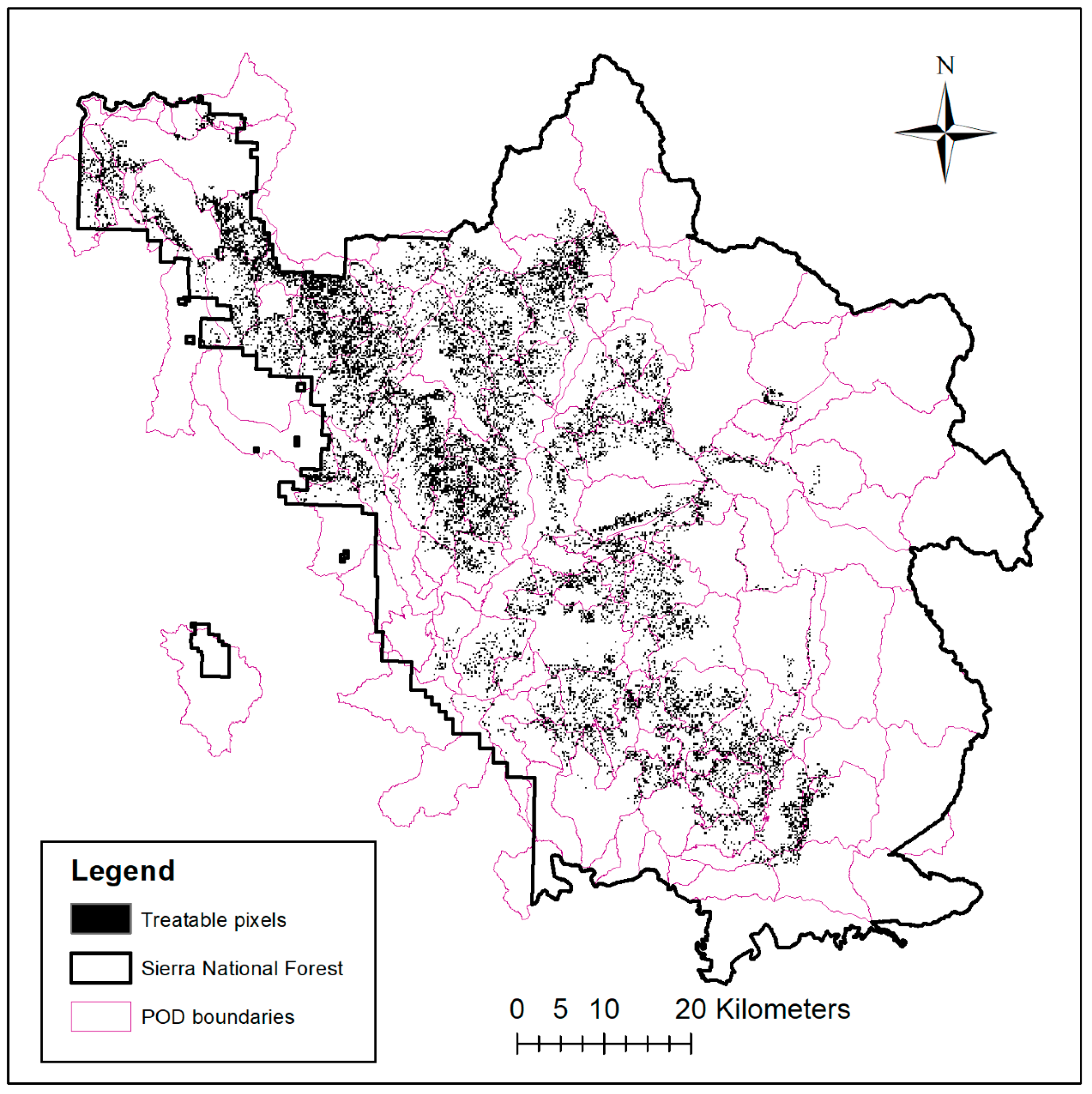
2.1. Case Study Location
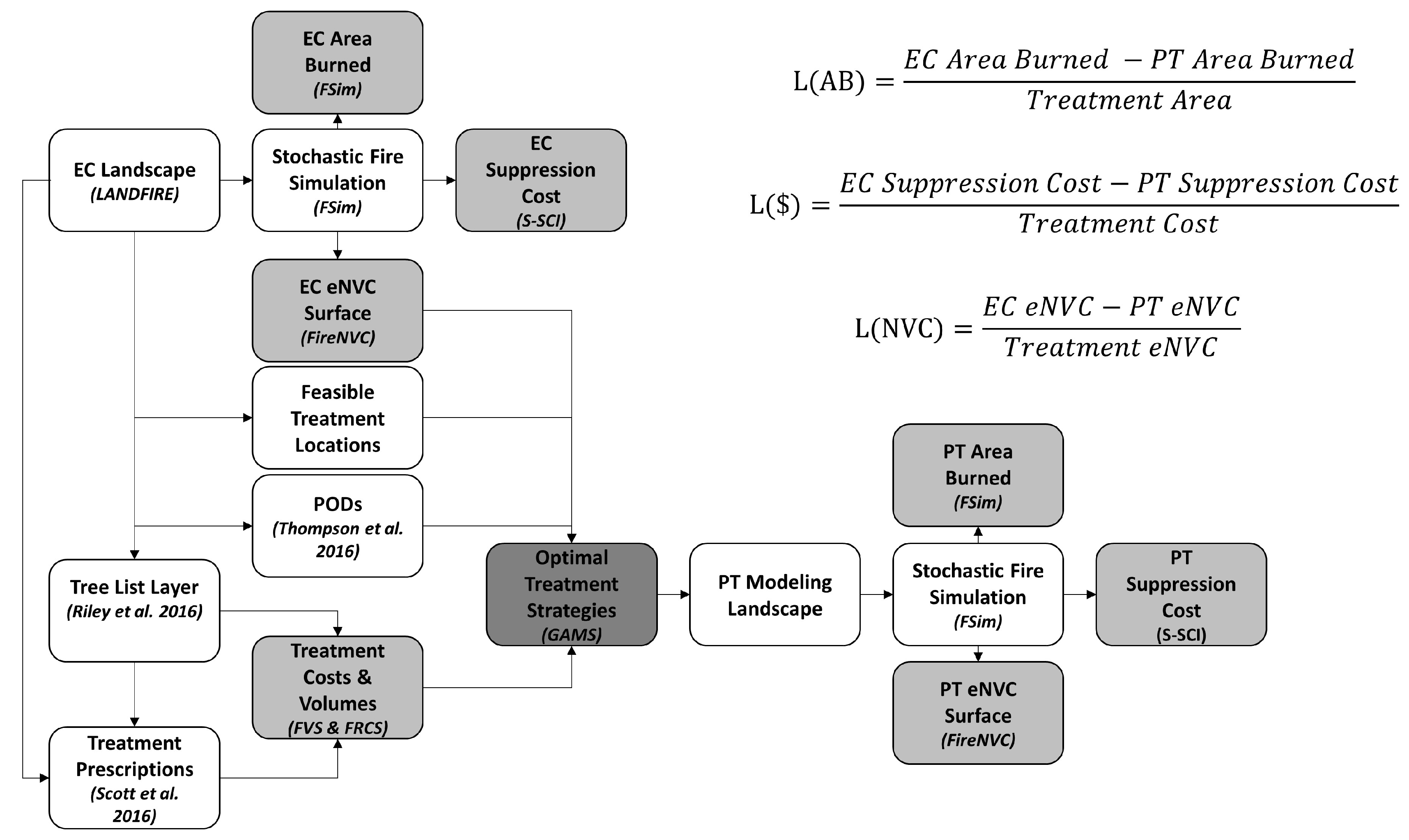
2.2. Model Workflow and Leverage Metrics
2.3. Fuel Treatment Eligibility, Prescription, and Cost Modeling
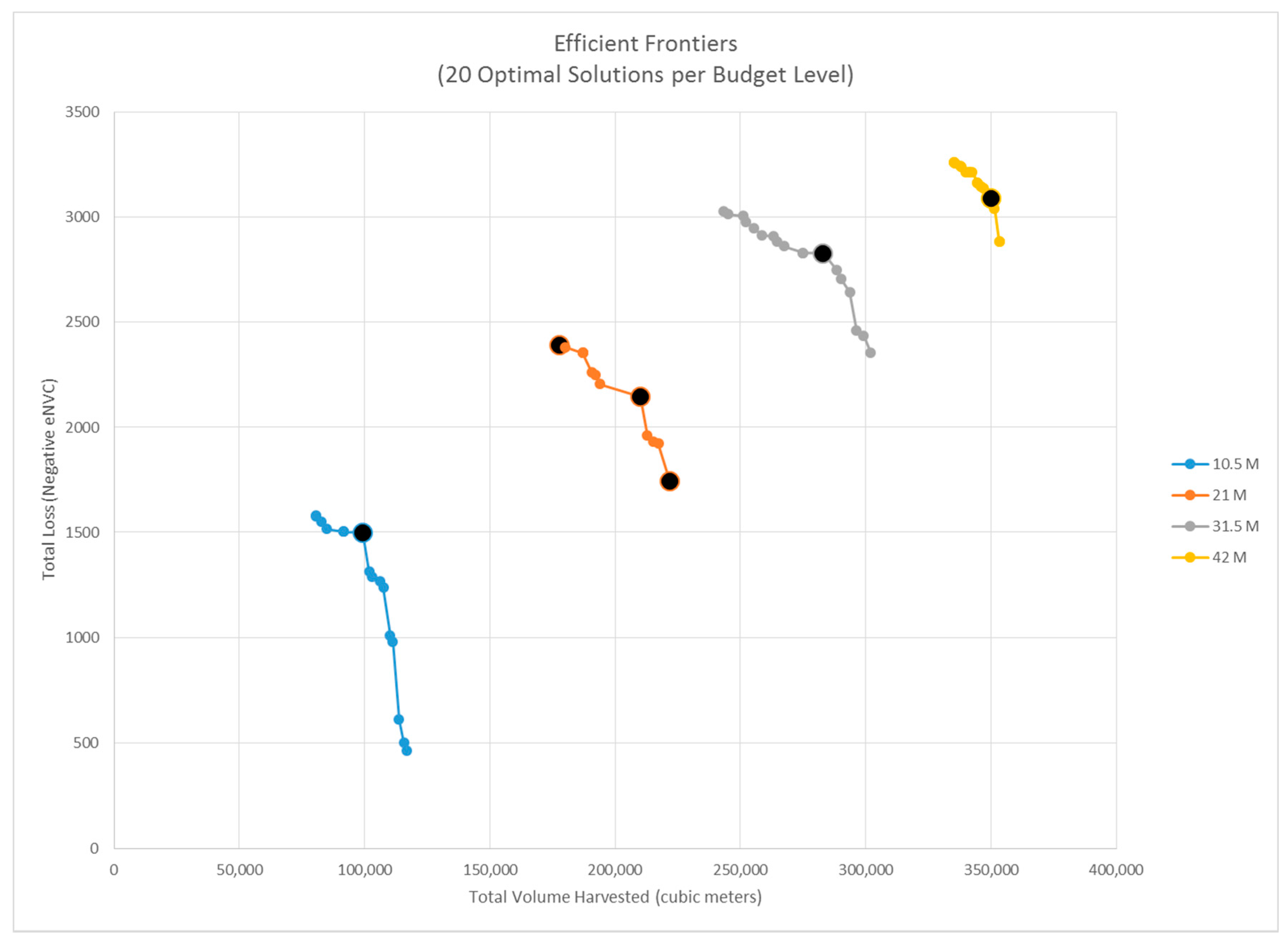
2.4. Treatment Strategy Optimization
| index for and set of feasible PODs | |
| B | maximum allowable budget |
| summed expected net value change for POD i | |
| total board foot volume harvested for POD i | |
| total treatment cost of POD i | |
| 0/1 variable; 1 if POD i is scheduled for treatment |
2.5. Stochastic Fire Simulation, Risk Assessment, and Suppression Cost Modeling
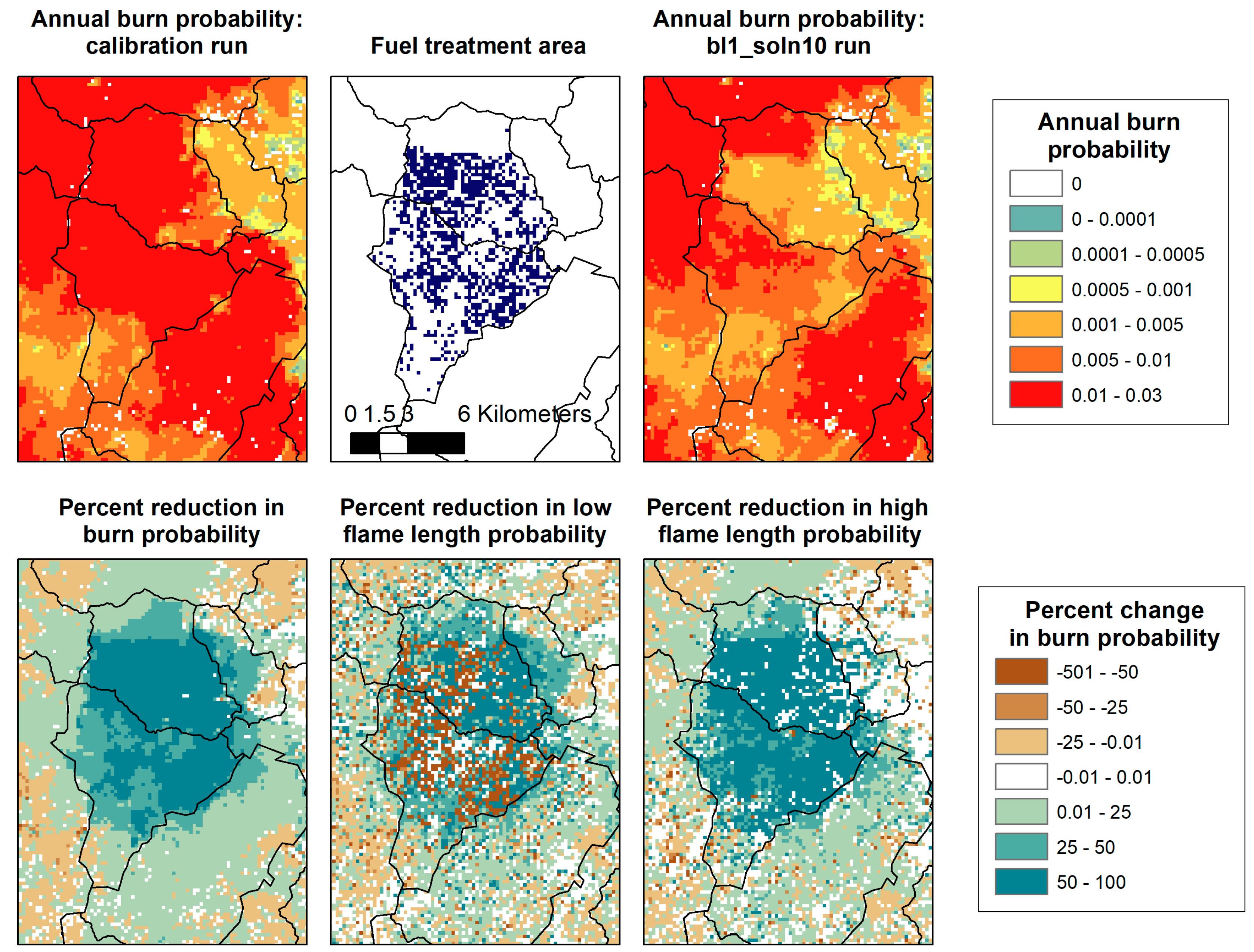
2.6. Fire-Treatment Encounters and Changes in Burn Probability
3. Results
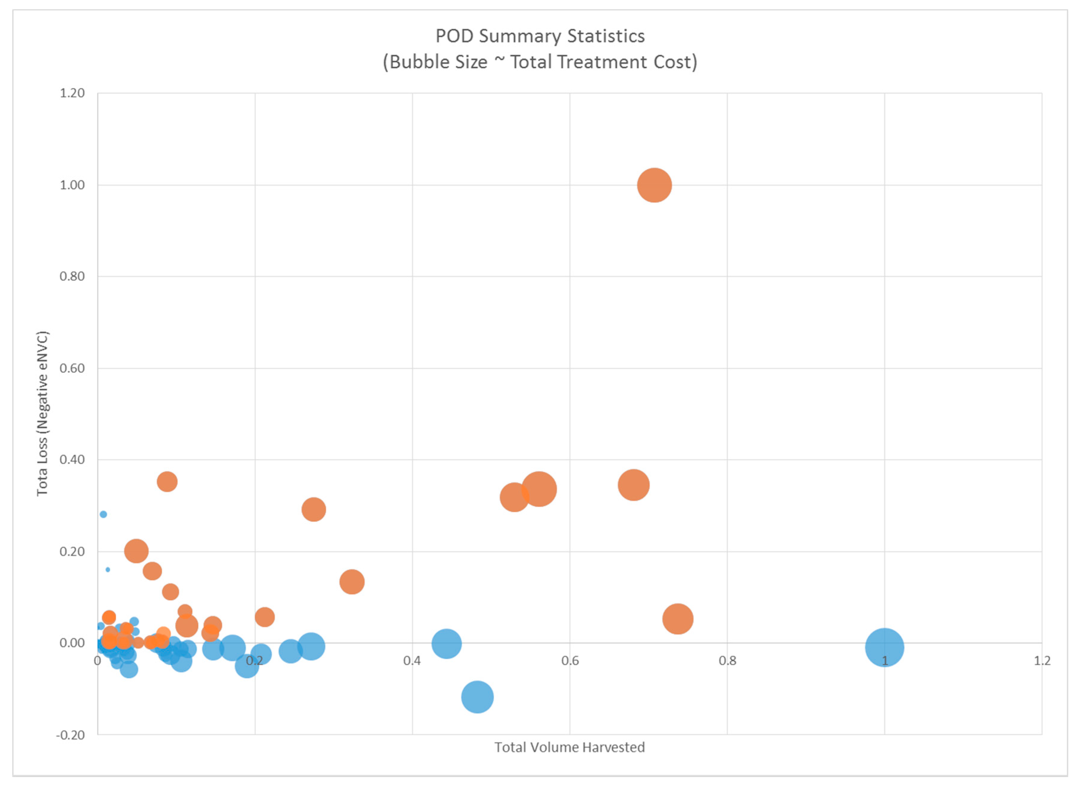
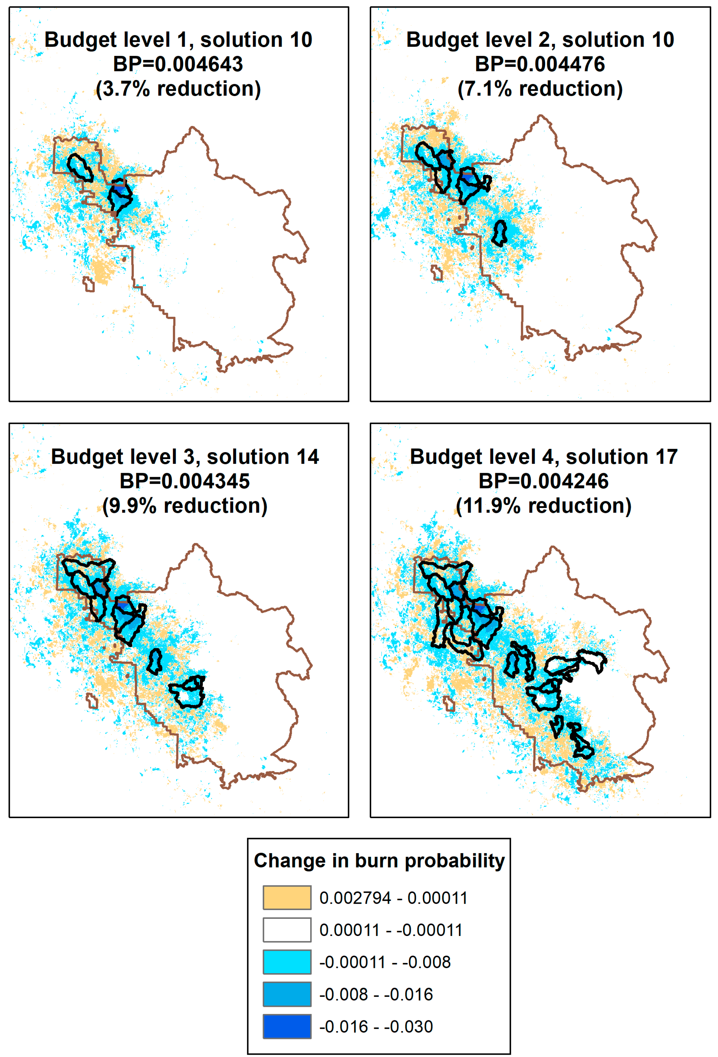
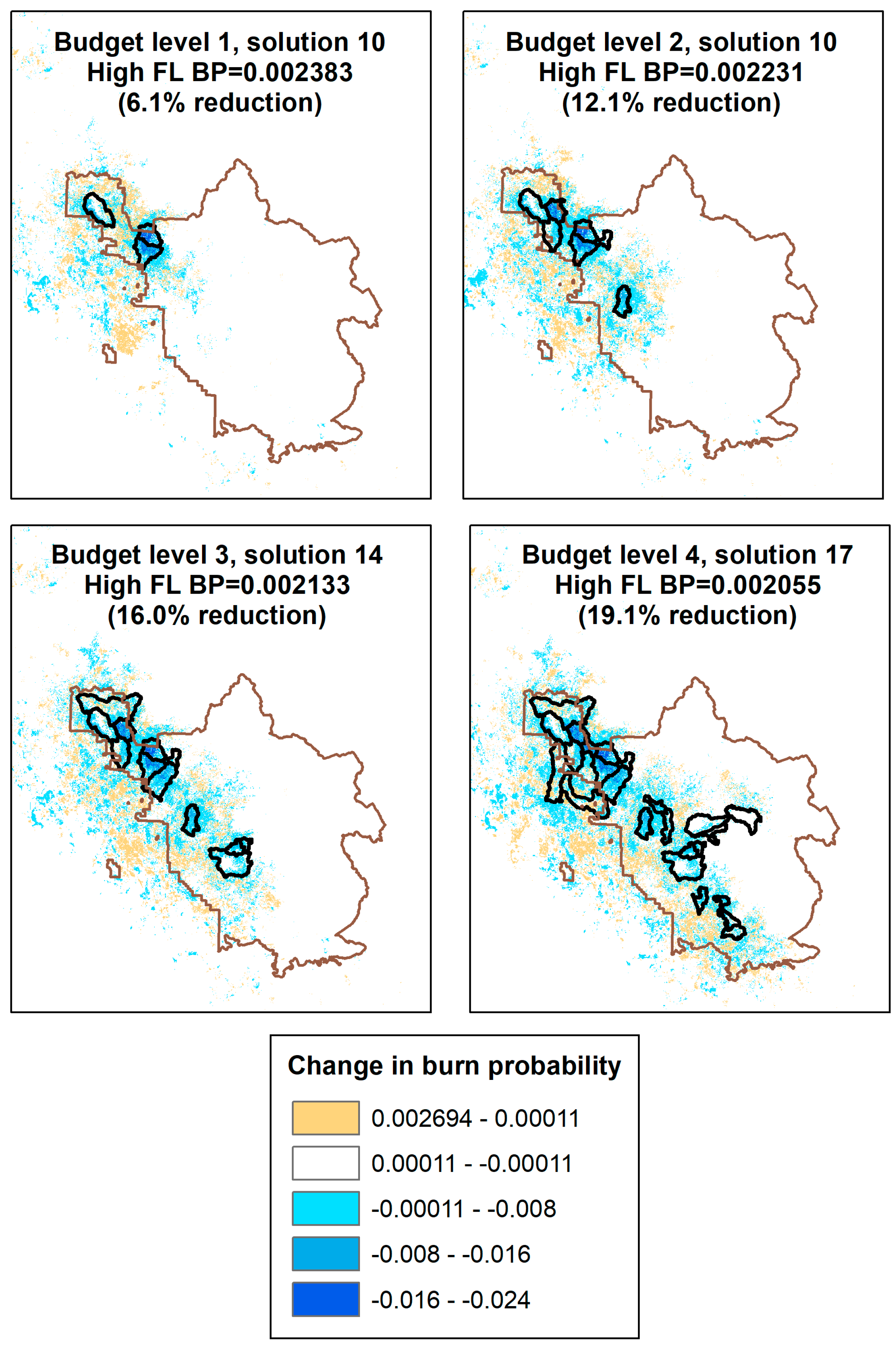
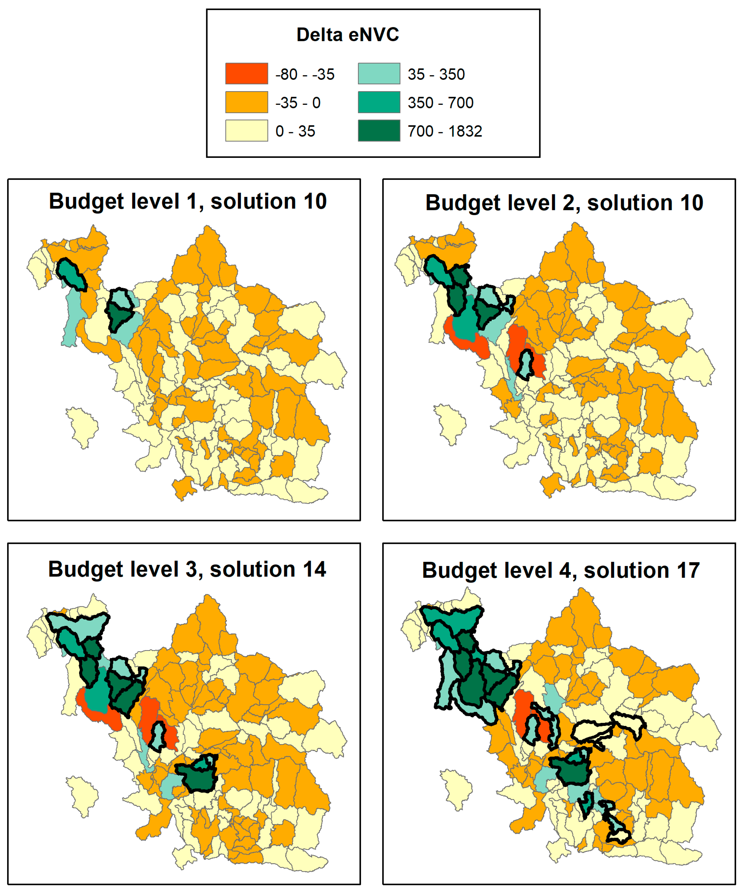
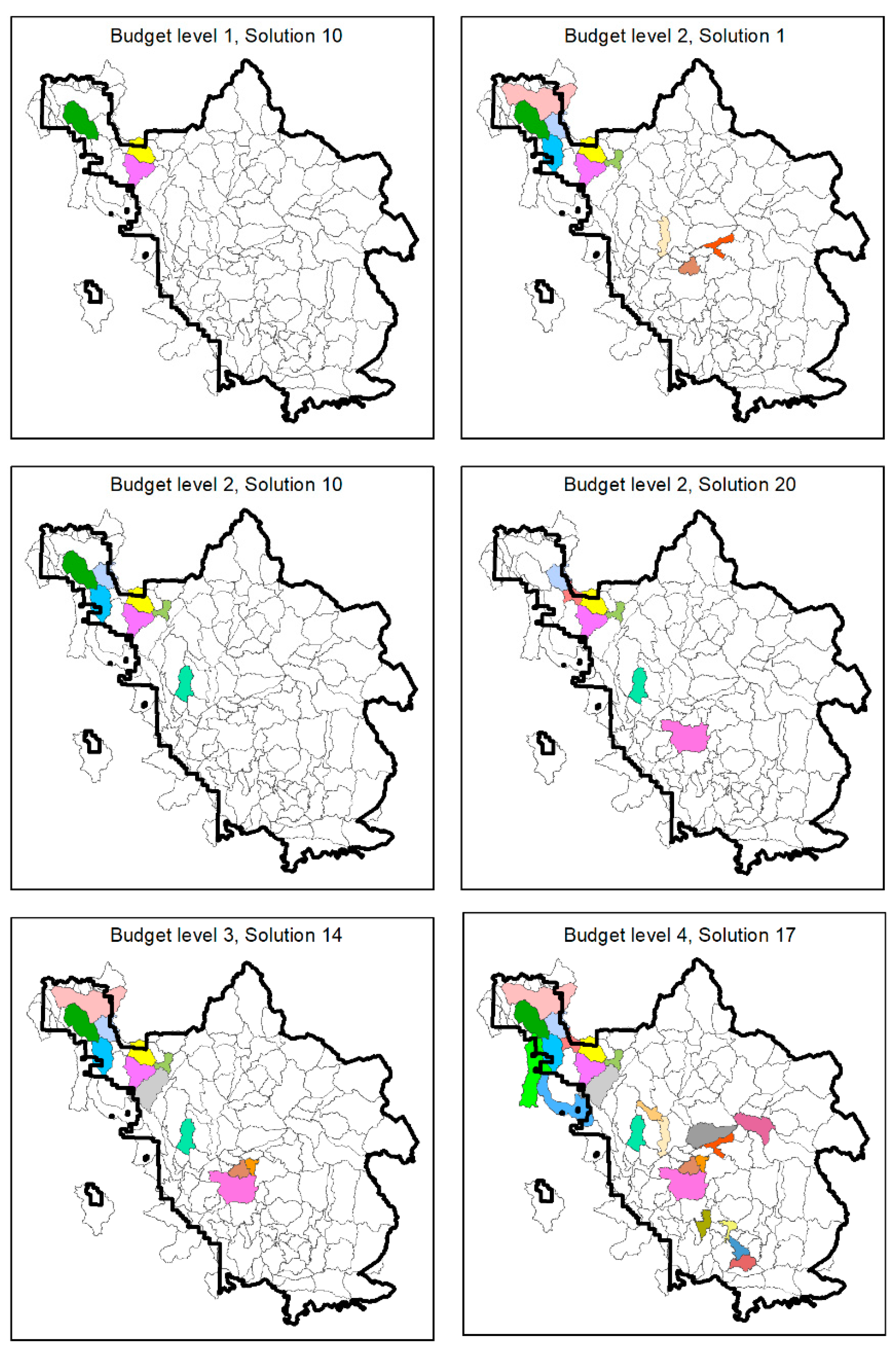
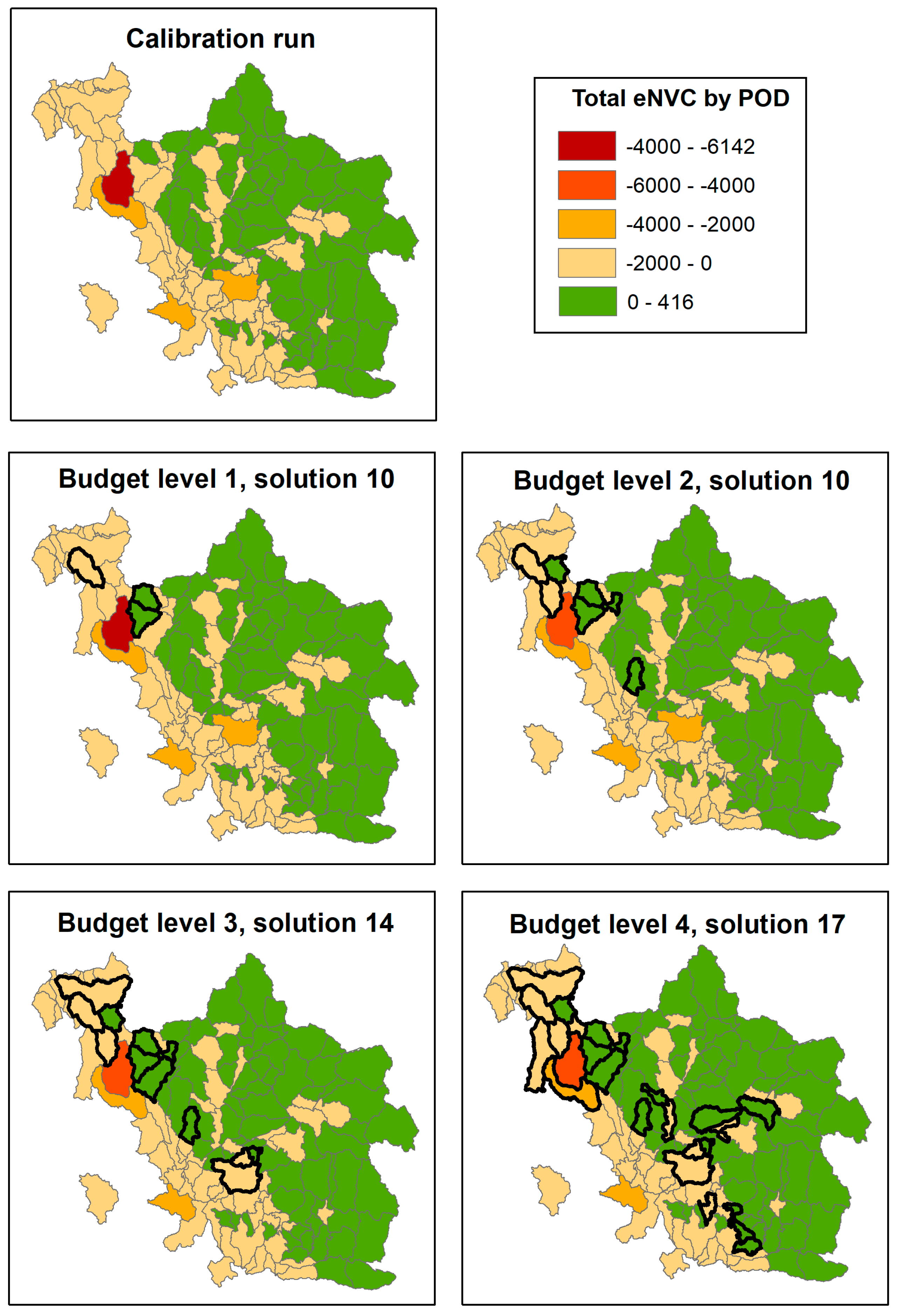
3.1. POD Summaries, Optimal Treatment Strategies, and Changes in Burn Probability
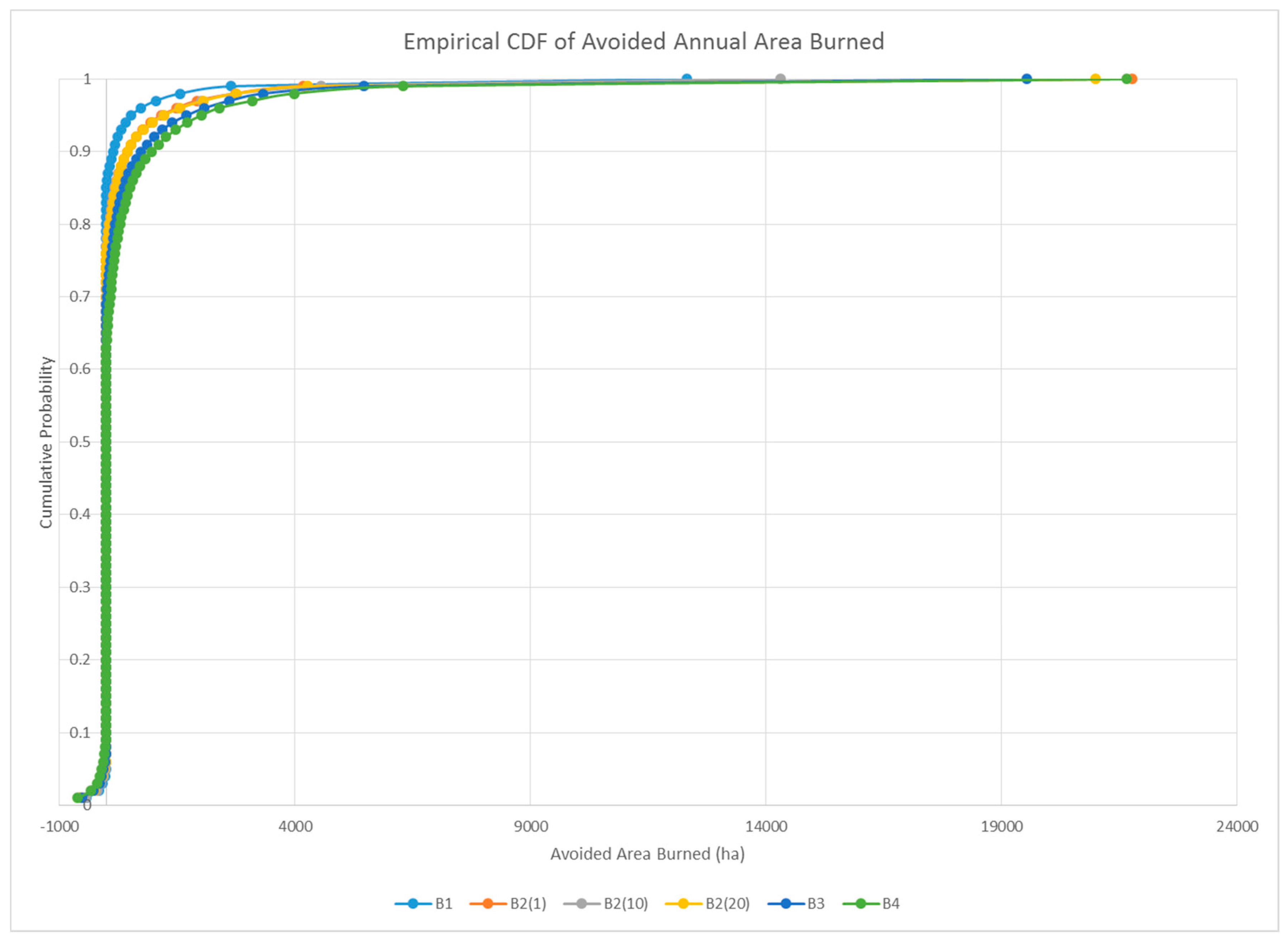
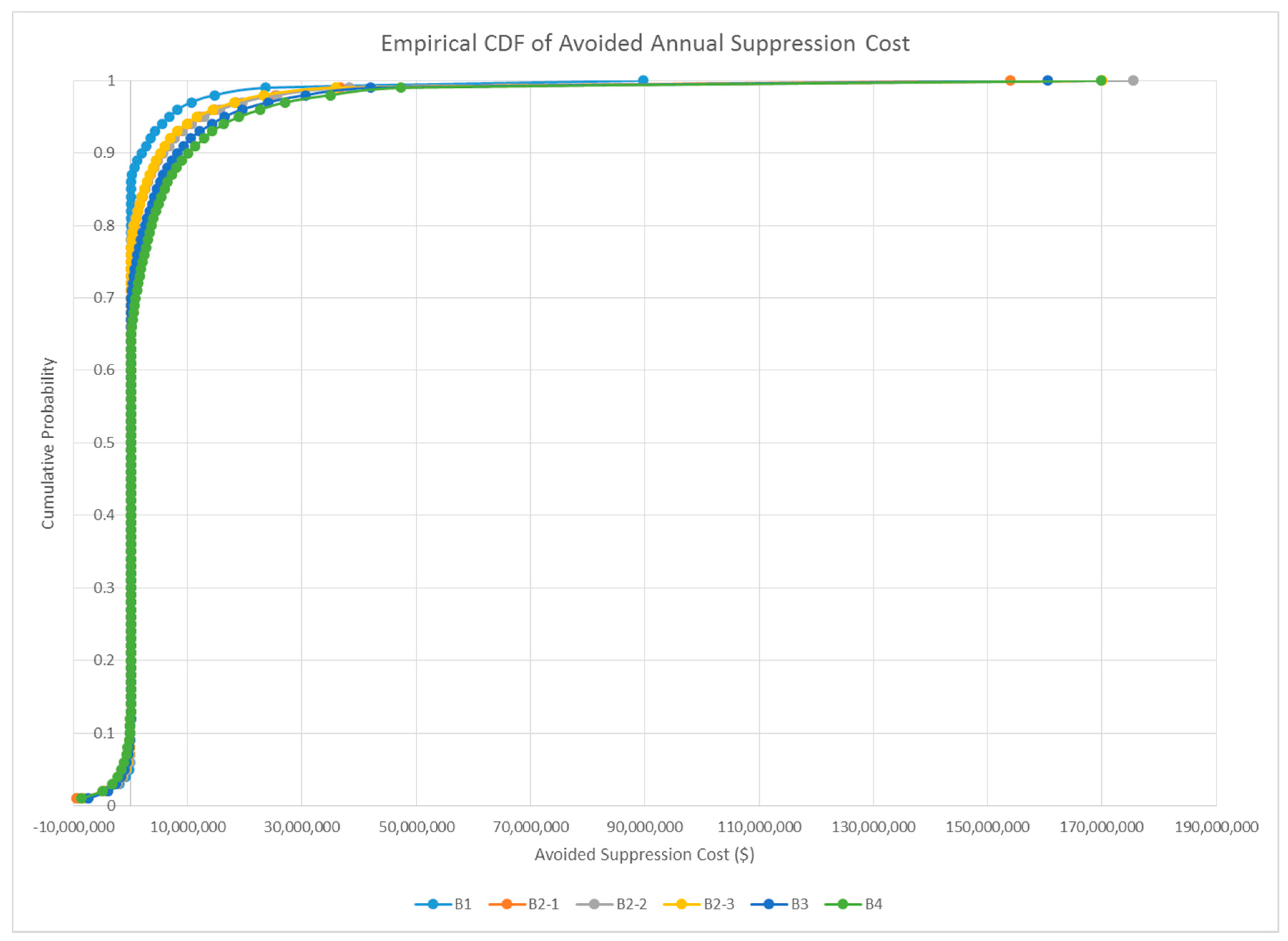
3.2. Encounter Rates and Leverage Metrics
4. Discussion
5. Conclusions
Acknowledgments
Author Contributions
Conflicts of Interest
References
- Abatzoglou, J.T.; Williams, A.P. Impact of anthropogenic climate change on wildfire across western US forests. Proc. Natl. Acad. Sci. USA 2016, 113, 11770–11775. [Google Scholar] [CrossRef] [PubMed]
- Jolly, W.M.; Cochrane, M.A.; Freeborn, P.H.; Holden, Z.A.; Brown, T.J.; Williamson, G.J.; Bowman, D.M. Climate-induced variations in global wildfire danger from 1979 to 2013. Nat. Commun. 2015, 6. [Google Scholar] [CrossRef] [PubMed]
- Riley, K.L.; Loehman, R.A. Mid-21st-century climate changes increase predicted fire occurrence and fire season length, Northern Rocky Mountains, United States. Ecosphere 2016, 7. [Google Scholar] [CrossRef]
- Syphard, A.D.; Massada, A.B.; Butsic, V.; Keeley, J.E. Land use planning and wildfire: Development policies influence future probability of housing loss. PLoS ONE 2013, 8, e71708. [Google Scholar] [CrossRef] [PubMed]
- Caggiano, M.D.; Tinkham, W.T.; Hoffman, C.; Cheng, A.S.; Hawbaker, T.J. High resolution mapping of development in the wildland-urban interface using object based image extraction. Heliyon 2016, 2, e00174. [Google Scholar] [CrossRef] [PubMed]
- Fusco, E.J.; Abatzoglou, J.T.; Balch, J.K.; Finn, J.T.; Bradley, B.A. Quantifying the human influence on fire ignition across the western USA. Ecol. Appl. 2016, 26, 2390–2401. [Google Scholar] [CrossRef] [PubMed]
- Gude, P.; Rasker, R.; Van den Noort, J. Potential for future development on fire-prone lands. J. For. 2008, 106, 198–205. [Google Scholar]
- Robinne, F.N.; Parisien, M.A.; Flannigan, M. Anthropogenic influence on wildfire activity in Alberta, Canada. Int. J. Wildland Fire 2016, 25, 1131–1143. [Google Scholar] [CrossRef]
- Theobald, D.M.; Romme, W.H. Expansion of the US wildland–urban interface. Landsc. Urban Plan. 2007, 83, 340–354. [Google Scholar] [CrossRef]
- Calkin, D.E.; Thompson, M.P.; Finney, M.A. Negative consequences of positive feedbacks in US wildfire management. For. Ecosyst. 2015, 2. [Google Scholar] [CrossRef]
- Collins, B.M.; Everett, R.G.; Stephens, S.L. Impacts of fire exclusion and recent managed fire on forest structure in old growth Sierra Nevada mixed-conifer forests. Ecosphere 2011, 2, 1–14. [Google Scholar] [CrossRef]
- Stephens, S.L.; Collins, B.M.; Biber, E.; Fulé, P.Z. US federal fire and forest policy: Emphasizing resilience in dry forests. Ecosphere 2016, 7. [Google Scholar] [CrossRef]
- Collins, R.D.; de Neufville, R.; Claro, J.; Oliveira, T.; Pacheco, A.P. Forest fire management to avoid unintended consequences: A case study of Portugal using system dynamics. J. Environ. Manag. 2013, 130, 1–9. [Google Scholar] [CrossRef] [PubMed]
- Curt, T.; Frejaville, T. Wildfire policy in Mediterranean France: How far is it efficient and sustainable? Risk Anal. 2017. [Google Scholar] [CrossRef] [PubMed]
- Olson, R.L.; Bengston, D.N.; DeVaney, L.A.; Thompson, T.A. Wildland Fire Management Futures: Insights from a Foresight Panel; Gen. Tech. Rep. NRS-152; U.S. Department of Agriculture, Forest Service, Northern Research Station: Newtown Square, PA, USA, 2015; 44p.
- Schoennagel, T.; Balch, J.K.; Brenkert-Smith, H.; Dennison, P.E.; Harvey, B.J.; Krawchuk, M.A.; Mietkiewicz, M.; Morgan, P.; Moritz, M.A.; Rasker, R.; et al. Adapt to more wildfire in western North American forests as climate changes. Proc. Natl. Acad. Sci. USA 2017, 114, 4582–4590. [Google Scholar] [CrossRef] [PubMed]
- Balch, J.K.; Bradley, B.A.; Abatzoglou, J.T.; Nagy, R.C.; Fusco, E.J.; Mahood, A.L. Human-started started wildfires expand the fire niche across the United States. Proc. Natl. Acad. Sci. USA 2017, 114, 2946–2951. [Google Scholar] [CrossRef] [PubMed]
- Prestemon, J.P.; Butry, D.T.; Thomas, D.S. The net benefits of human-ignited wildfire forecasting: The case of tribal land units in the United States. Int. J. Wildland Fire 2016, 25, 390–402. [Google Scholar] [CrossRef] [PubMed]
- North, M.P.; Stephens, S.L.; Collins, B.M.; Agee, J.K.; Aplet, G.; Franklin, J.F.; Fulé, P.Z. Reform forest fire management. Science 2015, 349, 1280–1281. [Google Scholar] [CrossRef] [PubMed]
- Haight, R.G.; Fried, J.S. Deploying wildland fire suppression resources with a scenario-based standard response model. INFOR Inf. Syst. Oper. Res. 2007, 45, 31–39. [Google Scholar] [CrossRef]
- Meyer, M.D.; Roberts, S.L.; Wills, R.; Brooks, M.; Winford, E.M. Principles of Effective USA Federal Fire Management Plans. Fire Ecol. 2015, 11. [Google Scholar] [CrossRef]
- Omi, P.N. Theory and practice of wildland fuels management. Curr. For. Rep. 2015, 1, 100–117. [Google Scholar] [CrossRef]
- Fernandes, P.M. Empirical support for the use of prescribed burning as a fuel treatment. Curr. For. Rep. 2015, 1, 118–127. [Google Scholar] [CrossRef]
- Agee, J.K.; Skinner, C.N. Basic principles of forest fuel reduction treatments. For. Ecol. Manag. 2005, 211, 83–96. [Google Scholar] [CrossRef]
- Cochrane, M.A.; Moran, C.J.; Wimberly, M.C.; Baer, A.D.; Finney, M.A.; Beckendorf, K.L.; Eidenshink, J.; Zhu, Z. Estimation of wildfire size and risk changes due to fuels treatments. Int. J. Wildland Fire 2012, 21, 357–367. [Google Scholar] [CrossRef]
- Finney, M.A.; McHugh, C.W.; Grenfell, I.C. Stand-and landscape-level effects of prescribed burning on two Arizona wildfires. Can. J. For. Res. 2005, 35, 1714–1722. [Google Scholar] [CrossRef]
- Graham, R.T.; Jain, T.B.; Loseke, M. Fuel Treatments, Fire Suppression, and Their Interaction with Wildfire and Its Impacts: The Warm Lake Experience during the Cascade Complex of Wildfires in Central Idaho, 2007; Gen. Tech. Rep. RMRS-GTR-229; U.S. Department of Agriculture, Forest Service, Rocky Mountain Research Station: Fort Collins, CO, USA, 2009; 36p.
- Moghaddas, J.J.; Craggs, L. A fuel treatment reduces fire severity and increases suppression efficiency in a mixed conifer forest. Int. J. Wildland Fire 2008, 16, 673–678. [Google Scholar] [CrossRef]
- Snider, G.; Daugherty, P.J.; Wood, D. The irrationality of continued fire suppression: An avoided cost analysis of fire hazard reduction treatments versus no treatment. J. For. 2006, 104, 431–437. [Google Scholar]
- Taylor, M.H.; Sanchez Meador, A.J.; Kim, Y.S.; Rollins, K.; Will, H. The economics of ecological restoration and hazardous fuel reduction treatments in the ponderosa pine forest ecosystem. For. Sci. 2015, 61, 988–1008. [Google Scholar] [CrossRef]
- Thompson, M.P.; Vaillant, N.M.; Haas, J.R.; Gebert, K.M.; Stockmann, K.D. Quantifying the potential impacts of fuel treatments on wildfire suppression costs. J. For. 2013, 111, 49–58. [Google Scholar] [CrossRef]
- Campbell, J.L.; Harmon, M.E.; Mitchell, S.R. Can fuel-reduction treatments really increase forest carbon storage in the western US by reducing future fire emissions? Front. Ecol. Environ. 2012, 10, 83–90. [Google Scholar] [CrossRef]
- North, M.; Brough, A.; Long, J.; Collins, B.; Bowden, P.; Yasuda, D.; Miller, J.; Sugihara, N. Constraints on mechanized treatment significantly limit mechanical fuels reduction extent in the Sierra Nevada. J. For. 2015, 113, 40–48. [Google Scholar] [CrossRef]
- Rhodes, J.J.; Baker, W.L. Fire probability, fuel treatment effectiveness and ecological tradeoffs in western US public forests. Open For. Sci. J. 2008, 1, 1–7. [Google Scholar]
- Thompson, M.; Anderson, N. Modeling fuel treatment impacts on fire suppression cost savings: A review. Calif. Agric. 2015, 69, 164–170. [Google Scholar] [CrossRef]
- Vaillant, N.M.; Reinhardt, E.D. An Evaluation of the Forest Service Hazardous Fuels Treatment Program—Are We Treating Enough to Promote Resiliency or Reduce Hazard? J. For. 2017, 115, 300–308. [Google Scholar] [CrossRef]
- Collins, B.M.; Stephens, S.L.; Moghaddas, J.J.; Battles, J. Challenges and approaches in planning fuel treatments across fire-excluded forested landscapes. J. For. 2010, 108, 24–31. [Google Scholar]
- Finney, M.A. A computational method for optimising fuel treatment locations. Int. J. Wildland Fire 2008, 16, 702–711. [Google Scholar] [CrossRef]
- Loudermilk, E.L.; Stanton, A.; Scheller, R.M.; Dilts, T.E.; Weisberg, P.J.; Skinner, C.; Yang, J. Effectiveness of fuel treatments for mitigating wildfire risk and sequestering forest carbon: A case study in the Lake Tahoe Basin. For. Ecol. Manag. 2014, 323, 114–125. [Google Scholar] [CrossRef]
- Barnett, K.; Parks, S.A.; Miller, C.; Naughton, H.T. Beyond fuel treatment effectiveness: Characterizing Interactions between fire and treatments in the US. Forests 2016, 7, 237. [Google Scholar] [CrossRef]
- Boer, M.M.; Sadler, R.J.; Wittkuhn, R.S.; McCaw, L.; Grierson, P.F. Long-term impacts of prescribed burning on regional extent and incidence of wildfires—Evidence from 50 years of active fire management in SW Australian forests. For. Ecol. Manag. 2009, 259, 132–142. [Google Scholar] [CrossRef]
- Price, O.F.; Pausas, J.G.; Govender, N.; Flannigan, M.; Fernandes, P.M.; Brooks, M.L.; Bird, R.B. Global patterns in fire leverage: The response of annual area burnt to previous fire. Int. J. Wildland Fire 2015, 24, 297–306. [Google Scholar] [CrossRef]
- Cary, G.J.; Davies, I.D.; Bradstock, R.A.; Keane, R.E.; Flannigan, M.D. Importance of fuel treatment for limiting moderate-to-high intensity fire: Findings from comparative fire modelling. Landsc. Ecol. 2017, 32, 1473–1483. [Google Scholar] [CrossRef]
- Ager, A.A.; Day, M.A.; Vogler, K. Production possibility frontiers and socioecological tradeoffs for restoration of fire adapted forests. J. Environ. Manag. 2016, 176, 157–168. [Google Scholar] [CrossRef] [PubMed]
- Stevens, J.T.; Collins, B.M.; Long, J.W.; North, M.P.; Prichard, S.J.; Tarnay, L.W.; White, A.M. Evaluating potential trade-offs among fuel treatment strategies in mixed-conifer forests of the Sierra Nevada. Ecosphere 2016, 7. [Google Scholar] [CrossRef]
- Vogler, K.C.; Ager, A.A.; Day, M.A.; Jennings, M.; Bailey, J.D. Prioritization of forest restoration projects: Tradeoffs between wildfire protection, ecological restoration and economic objectives. Forests 2015, 6, 4403–4420. [Google Scholar] [CrossRef]
- Schultz, C.A.; Jedd, T.; Beam, R.D. The Collaborative Forest Landscape Restoration Program: A history and overview of the first projects. J. For. 2012, 110, 381–391. [Google Scholar] [CrossRef]
- Collaborative Forest Landscape Restoration Program Results. Available online: https://www.fs.fed.us/restoration/CFLRP/results.shtml (accessed on 3 October 2017).
- Collaborative Forest Landscape Restoration Program Projects. Available online: https://www.fs.fed.us/restoration/CFLRP/guidance.shtml (accessed on 3 October 2017).
- Scott, J.H.; Thompson, M.P.; Calkin, D.E. A Wildfire Risk Assessment Framework for Land and Resource Management; Gen. Tech. Rep. RMRS-GTR-315; U.S. Department of Agriculture, Forest Service, Rocky Mountain Research Station: Fort Collins, CO, USA, 2013; 83p.
- Thompson, M.P.; Haas, J.R.; Gilbertson-Day, J.W.; Scott, J.H.; Langowski, P.; Bowne, E.; Calkin, D.E. Development and application of a geospatial wildfire exposure and risk calculation tool. Environ. Model. Softw. 2015, 63, 61–72. [Google Scholar] [CrossRef]
- Hand, M.S.; Thompson, M.P.; Calkin, D.E. Examining heterogeneity and wildfire management expenditures using spatially and temporally descriptive data. J. For. Econ. 2016, 22, 80–102. [Google Scholar] [CrossRef]
- Thompson, M.P. Decision making under uncertainty: Recommendations for the Wildland Fire Decision Support System (WFDSS). In Proceedings of the Large Wildland Fires Conference, Missoula, MT, USA, 19–23 May 2014; Keane, R.E., Jolly, W.M., Parsons, R., Riley, K.L., Eds.; USDA Forest Service, Rocky Mountain Research Station Proc.: Missoula, MT, USA, 2015. RMRS-P-73. [Google Scholar]
- Scott, J.H.; Thompson, M.P.; Gilbertson-Day, J.W. Examining alternative fuel management strategies and the relative contribution of National Forest System land to wildfire risk to adjacent homes—A pilot assessment on the Sierra National Forest, California, USA. For. Ecol. Manag. 2016, 362, 29–37. [Google Scholar] [CrossRef]
- Thompson, M.P.; Bowden, P.; Brough, A.; Scott, J.H.; Gilbertson-Day, J.W.; Taylor, A.; Anderson, J.; Haas, J.R. Application of Wildfire Risk Assessment Results to Wildfire Response Planning in the Southern Sierra Nevada, California, USA. Forests 2016, 7, 64. [Google Scholar] [CrossRef]
- Riley, K.L.; Thompson, M.P.; Scott, J.H.; Gilbertson-Day, J.G. A model-based framework to evaluate alternative wildfire suppression strategies. Resources 2017. in review. [Google Scholar]
- The Sierra National Forest. Available online: https://www.fs.usda.gov/sierra/ (accessed on 3 October 2017).
- Landscape Fire and Resource Management Planning Tools (LANDFIRE). Available online: https://www.landfire.gov/index.php (accessed on 3 October 2017).
- Dinkey Collaborative Landscape Restoration Strategy. Available online: https://www.fs.usda.gov/Internet/FSE_DOCUMENTS/stelprdb5351832.pdf (accessed on 3 October 2017).
- Short, K.C. A spatial database of wildfires in the United States, 1992–2011. Earth Syst. Sci. Data 2014, 6, 1–27. [Google Scholar] [CrossRef]
- Ballard, C.; Ballard, K.; Goss, J.; Rojas, R.; Tolmie, D.; Sierra National Forest Staff, CA, USA. Personal communication, 2016.
- Wei, Y.; Thompson, M.P.; Haas, J.; Dillon, G. Spatial optimization of operationally relevant large fire confine and point protection strategies: model development and test cases. Can. J. For. Res. 2017. in revisions. [Google Scholar]
- Riley, K.L.; Grenfell, I.C.; Finney, M.A. Mapping forest vegetation for the western United States using modified random forests imputation of FIA forest plots. Ecosphere 2016, 7. [Google Scholar] [CrossRef]
- Forest Vegetation Simulator. Available online: https://www.fs.fed.us/fvs/ (accessed on 3 October 2017).
- Fuel Reduction Cost Simulator. Available online: http://www.fs.fed.us/pnw/data/frcs/frcs.shtml (accessed on 3 October 2017).
- Calkin, D.; Gebert, K. Modeling fuel treatment costs on Forest Service lands in the western United States. West. J. Appl. For. 2006, 21, 217–221. [Google Scholar]
- Gross Domestic Product: Implicit Price Deflator. Available online: https://fred.stlouisfed.org/data/GDPDEF.txt (accessed on 3 October 2017).
- Finney, M.A.; McHugh, C.W.; Grenfell, I.C.; Riley, K.L.; Short, K.C. A simulation of probabilistic wildfire risk components for the continental United States. Stoch. Environ. Res. Risk Assess. 2011, 25, 973–1000. [Google Scholar] [CrossRef]
- Scott, J.H.; Thompson, M.P.; Gilbertson-Day, J.W. Exploring how alternative mapping approaches influence fireshed assessment and human community exposure to wildfire. GeoJournal 2017, 82, 201–215. [Google Scholar] [CrossRef]
- Jolly, M.; Missoula Fire Sciences Laboratory, Rocky Mountain Research Station, Missoula, MT, USA. Personal communication, 2014.
- Grenfell, I.C.; Finney, M.A.; Jolly, W.M. Simulating spatial and temporally related fire weather. In Proceedings of the VI International Conference on Forest Fire Research, Coimbra, Portugal, 15–18 November 2010; Viegas, D., Ed.; University of Coimbra: Coimbra, Portugal, 2010; p. 9. [Google Scholar]
- Finney, M.A. Fire growth using minimum travel time methods. Can. J. For. Res. 2002, 32, 1420–1424. [Google Scholar] [CrossRef]
- Scott, J.H.; Reinhardt, E.D. Assessing Crown Fire Potential by Linking Models of Surface and Crown Fire Behavior; USDA Forest Service Research Paper; U.S. Department of Agriculture, Forest Service, Rocky Mountain Research Station: Fort Collins, CO, USA, 2001.
- Finney, M.; Grenfell, I.C.; McHugh, C.W. Modeling containment of large wildfires using generalized linear mixed-model analysis. For. Sci. 2009, 55, 249–255. [Google Scholar]
- Scott, J.H.; Burgan, R.E. Standard Fire Behavior Fuel Models: A Comprehensive Set for Use with Rothermel’s Surface Fire Spread Model; General Technical Report RMRS-GTR-153; USDA Forest Service, Rocky Mountain Research Station: Fort Collins, CO, USA, 2005.
- Gebert, K.M.; Calkin, D.E.; Yoder, J. Estimating suppression expenditures for individual large wildland fires. West. J. Appl. For. 2007, 22, 188–196. [Google Scholar]
- Wildland Fire Decision Support System Data Downloads. Available online: http://wfdss.usgs.gov/wfdss/WFDSS_Data_Downloads.shtml (accessed on 3 October 2017).
- Hogland, J.; Anderson, N. Function Modeling Improves the Efficiency of Spatial Modeling Using Big Data from Remote Sensing. Big Data Cogn. Comput. 2017, 1, 3. [Google Scholar] [CrossRef]
- The R Project for Statistical Computing. Available online: https://www.r-project.org/ (accessed on 3 October 2017).
- Jones, K.W.; Cannon, J.B.; Saavedra, F.A.; Kampf, S.K.; Addington, R.N.; Cheng, A.S.; MacDonald, L.H.; Wilson, C.; Wolk, B. Return on investment from fuel treatments to reduce severe wildfire and erosion in a watershed investment program in Colorado. J. Environ. Manag. 2017, 198, 66–77. [Google Scholar] [CrossRef] [PubMed]
- Ager, A.A.; Vaillant, N.M.; McMahan, A. Restoration of fire in managed forests: A model to prioritize landscapes and analyze tradeoffs. Ecosphere 2013, 4, 1–19. [Google Scholar] [CrossRef]
- Sneeuwjagt, R.J.; Kline, T.S.; Stephens, S.L. Opportunities for improved fire use and management in California: Lessons from Western Australia. Fire Ecol. 2013, 9, 14–25. [Google Scholar]
- North, M.; Collins, B.M.; Stephens, S. Using fire to increase the scale, benefits, and future maintenance of fuels treatments. J. For. 2012, 110, 392–401. [Google Scholar] [CrossRef]
- Finney, M.A.; Seli, R.C.; McHugh, C.W.; Ager, A.A.; Bahro, B.; Agee, J.K. Simulation of long-term landscape-level fuel treatment effects on large wildfires. Int. J. Wildland Fire 2008, 16, 712–727. [Google Scholar] [CrossRef]
- Fried, J.S.; Potts, L.D.; Loreno, S.M.; Christensen, G.A.; Barbour, R.J. Inventory-based landscape-scale simulation of management effectiveness and economic feasibility with BioSum. J. For. 2016, 51, 6499–6514. [Google Scholar] [CrossRef]
- Riley, K.L.; Thompson, M.P. An uncertainty analysis of wildfire modeling. In Uncertainty in Natural Hazards: Modeling and Decision Support; Riley, K.L., Thompson, M.P., Webley, P., Eds.; Wiley and American Geophysical Union Books: New York, NY, USA, 2017; pp. 191–213. [Google Scholar]
- Barros, A.; Ager, A.; Day, M.; Preisler, H.; Spies, T.; White, E.; Pabst, R.; Olsen, K.; Platt, E.; Bailey, J.; et al. Spatiotemporal dynamics of simulated wildfire, forest management, and forest succession in central Oregon, USA. Ecol. Soc. 2017, 22. [Google Scholar] [CrossRef]
- O’Connor, C.D.; Calkin, D.E.; Thompson, M.P. An empirical machine learning method for predicting potential fire control locations for pre-fire planning and operational fire management. Int. J. Wildland Fire 2017, 26, 587–597. [Google Scholar]


| Treatment Scenario | Number of PODs Treated | Area Treated (ha) | Percent of Sierra National Forest Treated | Percent Reduction in Sierra National Forest Mean Burn Probability |
|---|---|---|---|---|
| Budget 1 | 3 | 4031 | 0.7% | 3.7% |
| Budget 2 (1) 1 | 10 | 8217 | 1.4% | 6.8% |
| Budget 2 (10) | 7 | 7922 | 1.4% | 7.2% |
| Budget 2 (20) | 7 | 7919 | 1.4% | 6.7% |
| Budget 3 | 12 | 12,114 | 2.1% | 9.9% |
| Budget 4 | 24 | 16,534 | 2.9% | 12.0% |
| Budget 1 | Budget 2 (1) | Budget 2 (10) | Budget 2 (20) | Budget 3 | Budget 4 | |
|---|---|---|---|---|---|---|
| Mean annual number of large fires | 2.40 | 2.38 | 2.38 | 2.38 | 2.36 | 2.35 |
| Proportion of fires that encountered a treatment | 0.07 | 0.16 | 0.14 | 0.14 | 0.22 | 0.31 |
| Mean treated area burned per fire (ha) | 9.12 | 20.18 | 19.27 | 18.71 | 28.20 | 36.71 |
| Proportion of fire seasons where fires encountered a treatment | 0.15 | 0.28 | 0.24 | 0.25 | 0.34 | 0.42 |
| Mean annual treated area burned (ha) | 21.85 | 47.77 | 45.55 | 44.19 | 66.23 | 85.60 |
| Budget 1 | Budget 2 (1) | Budget 2 (10) | Budget 2 (20) | Budget 3 | Budget 4 | |
|---|---|---|---|---|---|---|
| Mean reduction in annual area burned (ha) | 99.27 | 193.83 | 201.20 | 195.45 | 280.09 | 343.55 |
| Ratio of treated area burned to reduction in area burned | 11.23 | 10.03 | 10.91 | 10.93 | 10.45 | 9.92 |
| Budget 1 | Budget 2 (1) | Budget 2 (10) | Budget 2 (20) | Budget 3 | Budget 4 | |
|---|---|---|---|---|---|---|
| Mean annual avoided suppression costs ($M) | 0.72 | 1.67 | 1.79 | 1.60 | 2.50 | 2.99 |
| Percentile corresponding to full offset of treatment cost | 0.97 | 0.97 | 0.97 | 0.98 | 0.98 | 0.98 |
| Payback period (years) | 13.82 | 12.01 | 11.16 | 12.50 | 12.01 | 13.36 |
| Treatment revenue (total) to fully offset treatment cost in 10 years ($M) | $2.76 | $3.35 | $2.07 | $4.00 | $5.02 | $10.06 |
| Treatment revenue ($/cubic meter) to fully offset treatment cost in 10 years | $27.85 | $18.83 | $9.86 | $18.05 | $17.74 | $28.74 |
| Budget 1 | Budget 2 (1) | Budget 2 (10) | Budget 2 (20) | Budget 3 | Budget 4 | |
|---|---|---|---|---|---|---|
| L(AB) | 0.06 | 0.06 | 0.06 | 0.06 | 0.06 | 0.05 |
| L($) | 0.07 | 0.08 | 0.09 | 0.08 | 0.08 | 0.07 |
| L(NVC) | 2.94 | 3.05 | 2.66 | 2.54 | 2.85 | 2.86 |
© 2017 by the authors. Licensee MDPI, Basel, Switzerland. This article is an open access article distributed under the terms and conditions of the Creative Commons Attribution (CC BY) license (http://creativecommons.org/licenses/by/4.0/).
Share and Cite
Thompson, M.P.; Riley, K.L.; Loeffler, D.; Haas, J.R. Modeling Fuel Treatment Leverage: Encounter Rates, Risk Reduction, and Suppression Cost Impacts. Forests 2017, 8, 469. https://doi.org/10.3390/f8120469
Thompson MP, Riley KL, Loeffler D, Haas JR. Modeling Fuel Treatment Leverage: Encounter Rates, Risk Reduction, and Suppression Cost Impacts. Forests. 2017; 8(12):469. https://doi.org/10.3390/f8120469
Chicago/Turabian StyleThompson, Matthew P., Karin L. Riley, Dan Loeffler, and Jessica R. Haas. 2017. "Modeling Fuel Treatment Leverage: Encounter Rates, Risk Reduction, and Suppression Cost Impacts" Forests 8, no. 12: 469. https://doi.org/10.3390/f8120469
APA StyleThompson, M. P., Riley, K. L., Loeffler, D., & Haas, J. R. (2017). Modeling Fuel Treatment Leverage: Encounter Rates, Risk Reduction, and Suppression Cost Impacts. Forests, 8(12), 469. https://doi.org/10.3390/f8120469