Article

Impact of Climate Change on the Spatial Dynamics of Habitats Suitable for the Genus Clusia L. in Peru

by
Dennis Cieza-Tarrillo
1,
Jim J. Villena-Velásquez
1,2,
Neiser Vergara-Yrigoin
2,
José I. Pomiano-Mendoza
1,
Jeiner O. Rafael-Abanto
2,
Sivmny V. Valqui-Reina
1,
Sandy Chapa-Gonza
1,
Carlos Culqui-Arce
1,* and
Alex J. Vergara
1,*
1
Instituto de Investigación en Forestería y Ecosistemas Tropicales (INIFET), Escuela Profesional de Ingeniería Forestal, Universidad Nacional Toribio Rodríguez de Mendoza de Amazonas (UNTRM), Chachapoyas 01001, Peru
2
Grupo de Investigación en Gestión Sostenible, Genética y Tecnología Forestal (GIGESTFOR), Universidad Nacional Autónoma de Chota, Chota 06121, Peru
*
Authors to whom correspondence should be addressed.
Forests 2026, 17(9), 1126; https://doi.org/10.3390/f17091126
Submission received: 19 August 2026 / Revised: 15 September 2026 / Accepted: 17 September 2026 / Published: 20 September 2026

Abstract

Climate change is expected to reshape the climatic suitability of Neotropical plant taxa, particularly in topographically complex regions such as the tropical Andes, yet no nationwide assessment exists for the genus Clusia L. (Clusiaceae) in Peru. We modeled its current and future potential distribution using MaxEnt, based on 245 spatially thinned occurrence records (GBIF) and bioclimatic variables from WorldClim 2.1 selected through Pearson correlation and variance inflation factor filtering. Model complexity was tuned with ENMeval using spatial block cross-validation, and future projections were generated under the SSP2-4.5 and SSP5-8.5 scenarios for 2041–2060, 2061–2080, and 2081–2100 across three Global Climate Models. The model showed acceptable, stable performance (training AUC = 0.824, test AUC = 0.825), with elevation and precipitation seasonality (Bio15) as the leading predictors, together with Bio19 and Bio3 accounting for over 80% of the total contribution. Currently, only 16.61% of Peru is climatically suitable (medium–high) for the genus, concentrated discontinuously along Andean slopes and inter-Andean valleys. Both future scenarios project progressive contraction and fragmentation of suitable habitat, most severe under SSP5-8.5, where high-loss areas reach 50.43% of the evaluated territory by 2081–2100; these projections should be interpreted as plausible scenarios rather than validated forecasts, given the absence of independent data for future periods. Habitat gains were restricted to higher elevations, consistent with an altitudinal range shift. These results provide a coarse-scale spatial baseline that highlights broad patterns of climatic vulnerability for the genus, intended to guide exploratory conservation attention and future species-level research in the Andean region, rather than site-specific management decisions.

1. Introduction

Climate change alters the temperature and precipitation gradients that determine species distribution, particularly in regions where variations in these climatic variables act as limiting factors for species persistence [1,2]. These changes alter the climatic suitability for species, affecting their distribution patterns, survival, and population dynamics. As a result, altitudinal and latitudinal shifts, a reduction in climatically favorable areas, habitat fragmentation, and changes in the composition of biological communities may occur [1,3,4,5]. In tropical mountain ecosystems, these effects are more significant due to abrupt environmental gradients, high plant diversity, and species groups with limited distributions or those that depend on specific climatic conditions [4,6,7].
Peru is particularly vulnerable to these processes because it encompasses the western Amazon and the tropical Andes, two regions known for their high plant diversity, high endemism, and marked environmental heterogeneity [8,9]. The wide range of elevations, humidity gradients, and climatic diversity create conditions that favor a high abundance of Neotropical plants. In turn, these factors influence the differential responses of species to climate change, altering the extent and location of climatically favorable areas [10]. Therefore, assessing the potential distribution of plant taxa under future climate scenarios is essential for understanding how species might be redistributed, identifying areas of stability, contraction, or expansion of their potential habitat, and generating scientific information to support the planning of conservation strategies, biodiversity management, and decision-making in the face of the effects of climate change [8,10].
In this context, the genus Clusia L. (Clusiaceae) is one of the most representative taxa of Neotropical tropical forests due to its wide geographic distribution, high species diversity, and ability to occupy a wide variety of habitats, ranging from lowland rainforests to montane forests, where it plays an important role in the structure and functioning of these ecosystems [11,12,13]. It currently comprises more than 300 species distributed from southern Mexico, through Central America and the Antilles, to Colombia, Venezuela, Ecuador, Peru, Bolivia, and northern Argentina, with its main centers of diversification concentrated in the Amazon Basin and the tropical Andes [12,14,15]. Its species include trees, shrubs, epiphytes, and hemiepiphytes capable of colonizing Amazonian, montane, and premontane rainforests, reflecting high ecological plasticity and a wide distribution [13,16]. In Peru, the available information on the genus comes primarily from herbarium records, floristic inventories, and georeferenced biodiversity databases [17,18]. However, these records represent isolated observations of presence and are influenced by differences in botanical sampling effort across geographic regions, which may generate spatial gaps and biases in occurrence data [19,20]. Therefore, occurrence records alone may not fully represent the potential distribution of suitable habitats or future changes under climate scenarios.
Despite the ecological importance of the genus Clusia L., whose species contribute to the structure and functioning of tropical forests by providing essential resources for wildlife and other ecosystem components [11,12,13], as well as containing bioactive compounds of pharmaceutical and cosmetic interest, possessing ornamental value, participating in succession dynamics, and occupying various vegetation strata [11,12,13], its potential distribution in Peru remains insufficiently assessed from a spatial and climatic perspective. This gap limits the identification of priority areas for conservation, botanical exploration, and land-use planning [21], a situation that is particularly relevant in light of the environmental changes projected for the 21st century [22,23]. Furthermore, the lack of nationwide studies limits our understanding of the genus’s potential response to intermediate and high greenhouse gas emission scenarios, making it difficult to identify future changes in its potential distribution and to formulate conservation strategies based on scientific evidence [24].
Species distribution models allow for the estimation of areas of environmental suitability based on presence records and climatic variables [25], making them a useful tool for analyzing taxa with incomplete biogeographic information [26]. Consequently, various algorithms have been developed, including Generalized Linear Models (GLM), Generalized Additive Models (GAM), Random Forest (RF), Boosted Regression Trees (BRT), and MaxEnt, which differ in their data requirements, predictive capacity, and ecological applications [25]. Among these, MaxEnt has demonstrated robust performance when only presence records are available, a common situation in floristic studies and biodiversity databases [27]. However, its application requires controlling for the quality of occurrence records, spatial bias, redundancy among predictors, and model complexity in order to obtain ecologically consistent projections [28,29].
Temperature and moisture gradients related to vegetation distribution can be characterized using an appropriate climatic basis, which can be provided by the bioclimatic variables from WorldClim [30,31,32]. Likewise, future climate projections can be assessed using the Shared Socioeconomic Pathways (SSPs), which represent different trajectories of socioeconomic development associated with varying levels of greenhouse gas emissions and radiative forcing [33]. In particular, the SSP2-4.5 and SSP5-8.5 scenarios allow for a comparison between an intermediate scenario and a high-emissions scenario for the periods 2041–2060, 2061–2080, and 2081–2100. To reduce the uncertainty associated with climate projections, these were evaluated using three Global Climate Models (GCMs) [30,33,34].
In Peru, distribution models have been used in various studies to assess plant species and genera of ecological, forestry, or economic importance [35,36,37,38]. However, there is still no national assessment aimed at estimating the current and future potential distribution of the genus Clusia L. under the SSP2-4.5 and SSP5-8.5 scenarios. This gap limits our understanding of its potential redistribution in response to climate change and hinders the identification of priority areas for conservation, biodiversity monitoring, land-use planning, and the design of management strategies based on scientific evidence [39,40].
This study evaluated the current and future potential distribution of the genus Clusia L. in Peru using maximum entropy modeling, based on georeferenced occurrence records and bioclimatic variables from WorldClim. Future projections were analyzed under the SSP2-4.5 and SSP5-8.5 scenarios for the periods 2041–2060, 2061–2080, and 2081–2100. This allowed for the identification of climatically favorable areas, the estimation of potential changes in environmental suitability, and the generation of spatial evidence for the conservation and biogeographic research of the genus in Peru.

2. Materials and Methods

2.1. Study Area

The study area comprised the entire territory of Peru, located in the western part of South America (Figure 1A). Peru extends between latitudes 0°01′ and 18°21′ S and longitudes 68°39′ and 81°20′ W (Figure 1B). Covering an area of 1,285,216 km2, the country exhibits a pronounced altitudinal gradient, ranging from sea level to 6733 m above sea level, which contributes to its remarkable physiographic, climatic, and ecological heterogeneity [39,41,42].
Peruvian territory comprises three major natural regions (Coast, Highlands, and Rainforest), characterized by marked gradients in temperature, precipitation, and topography [43]. This environmental heterogeneity is reflected in the presence of 84 of Holdridge’s 104 life zones, as well as in a high diversity of terrestrial ecosystem conditions that support a rich flora and make Peru an ideal setting for assessing potential changes in species distribution under climate change scenarios [9,44,45]. Among the main ecosystems are Amazonian rainforests, montane and montane cloud forests, seasonally dry forests, and high-Andean scrublands and grasslands, whose distribution is primarily determined by altitudinal, climatic, and topographic gradients [46,47,48].
Climatic conditions vary significantly from one natural region to another. The Coast region has average annual precipitation ranging from 22 to 174 mm and average annual temperatures of 18 to 24 °C [49]; the Sierra region has average temperatures ranging from 7 to 18 °C and precipitation ranging from 570 to 1200 mm per year, with marked seasonality [50,51], while the Rainforest is characterized by average annual temperatures ranging from 24 to 27 °C and precipitation generally exceeding 2000 mm per year, which favors the development of extensive tropical rainforests [9]. This climatic variability is one of the main factors determining the distribution of vegetation and species throughout Peru.

2.2. Database Compilation

The georeferenced records of the genus Clusia L. in Peru were obtained from the Global Biodiversity Information Facility (GBIF) (https://www.gbif.org/es/) (accessed on 10 July 2026), with 961 occurrence points initially compiled. Subsequently, the nomenclatural authorship, the recognized scientific name, the synonyms, and the taxonomic rank of identification were reviewed. Finally, the names were standardized according to their current nomenclature to ensure the taxonomic and spatial consistency of the dataset used in the ecological modeling [52,53]. The removal of coordinates that were null, repeated, inverted, located in the ocean, or assigned to administrative centroids that did not match the location description was part of the geographic validation process [54,55]. This procedure resulted in the exclusion of 113 records due to incorrect geographic coordinates, 68 duplicate records, and 23 records located outside Peruvian territory, yielding 757 valid records. No explicit numerical threshold for coordinate uncertainty was applied; records were filtered based on geographic validation criteria and the availability of climate information, as described above. Furthermore, in order to reduce autocorrelation and bias related to road networks, urban areas, or regions with high sampling density, spatial filtering was applied using a minimum nearest-neighbor distance of 2 km, consistent with distances used in previous Neotropical plant SDM studies [19,56,57]; this step removed 512 additional records due to spatial clustering. As a result, a final dataset of 245 occurrence points was obtained for the development of the distribution models. Finally, the cleaned dataset was overlaid with bioclimatic variables, thereby yielding a set of unique occurrences that are taxonomically reliable and spatially independent, which was used to calibrate and validate MaxEnt [29,58].

2.3. Variable Selection and Processing

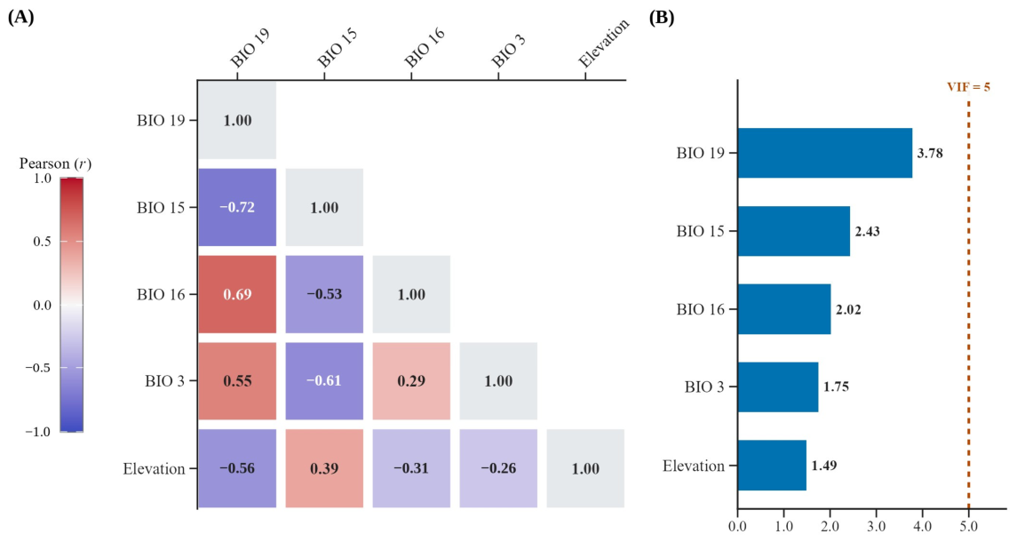
The environmental characterization was performed using the nineteen bioclimatic variables from WorldClim version 2.1 (https://worldclim.org), which cover the reference period from 1970 to 2000 and have a spatial resolution of 30 arcseconds. These data reveal annual and seasonal patterns, as well as extreme conditions related to temperature and precipitation, key factors in determining the distribution of tropical and mountain vegetation [59,60]. All raster datasets were cropped to the political boundaries of Peru and harmonized in terms of extent, origin, cell size, number of rows and columns, coordinate system, and units [32,61,62]. For the cartographic analysis, the data were projected into WGS 84 and resampled to a common grid of 250 m using bilinear interpolation; this process ensured that the layers coincided spatially, although this should not be interpreted as an improvement in the actual climatic resolution of the original ~1-km WorldClim data [63,64]. In addition, the quality of each predictor was verified by checking for discontinuities, outliers, coding errors, and empty cells. Climate values were then obtained for the cleaned-up locations and for a random selection of land cells [32,65,66]. The autocorrelation of variables was analyzed using Pearson’s correlation; variables with |r| ≥ 0.80 were excluded [67]. As an additional check, the variance inflation factor (VIF) was calculated, and variables with VIF ≥ 5 were successively removed until a stable set with VIF < 5 was obtained (Figure 2) [68]. The selection process avoided including variables derived from the same climatic signal simultaneously and prioritized predictors capable of representing water availability, thermal amplitude, and seasonality (Table 1) [65,69].

2.4. Selection of Climate Models for Future Prediction

To generate future projections of climate suitability, bioclimatic variables derived from the Coupled Model Intercomparison Project, Phase 6 (CMIP6) simulations available through WorldClim v2.1 were used; these data have been spatially downsampled and bias-corrected using the WorldClim v2.1 reference climate [32,70]. Three global climate models (GCMs) were selected: ACCESS-CM2, HadGEM3-GC31-LL, and MPI-ESM1-2-HR. For each GCM, climate suitability projections were carried out independently under the SSP2-4.5 and SSP5-8.5 scenarios for the periods 2041–2060, 2061–2080, and 2081–2100 [71,72,73]. The GCMs were selected based on the need to account for some of the structural uncertainty associated with climate projections, as well as the available evidence on the performance of CMIP6 models in South America. Regional evaluation studies have shown that GCM performance varies across subregions and climate variables, particularly in high-altitude regions with complex topography such as the Andes; therefore, no single model can be considered optimal for all climatic conditions [74,75,76]. The use of a multimodel ensemble made it possible to reduce dependence on a single climate scenario and account for the uncertainty associated with differences among global climate models (GCMs), providing a more robust representation of possible future climate conditions [77]. To integrate the projections from the three GCMs, the pixel-by-pixel median was used, generating a consensus climate projection for each scenario and period. This method served to reduce the influence of extreme values across models, thereby representing the central trend of the dataset. In addition, uncertainty was estimated using the per-cell standard deviation among GCMs, identifying areas of greater climate agreement or divergence [78]. To evaluate responses under contrasting climate forcing conditions, the CMIP6 SSP2-4.5 and SSP5-8.5 scenarios were considered, corresponding to intermediate and high radiative forcing trajectories, respectively [72].
The first describes an intermediate scenario in which radiative forcing stabilizes; the second, on the other hand, points to a trend of high emissions and increased warming by the end of the 21st century [73,79]. For each scenario, the periods 2041–2060, 2061–2080, and 2081–2100 were considered [80]. Future layers included only the variables retained during the current calibration and were subjected to the same clipping, alignment, reprojection, and unit checking. Likewise, the reference system, the land mask, the spatial extent, the map resolution, and the cell origin were kept constant [81]. Finally, MaxEnt was used to project each combination of scenario, model, and time period independently [82,83].

2.5. MaxEnt Modeling

The current and future distribution of Clusia L. was modeled in the R 4.6.0 environment using the maximum entropy (MaxEnt) algorithm, which is widely used to estimate environmental suitability and the potential distribution of species based on presence records and environmental variables [84,85]. Model calibration, evaluation, and selection were performed using the ENMeval 2.0.5.2 software package, which is designed to facilitate the reproducible evaluation of ecological niche models and the selection of optimal MaxEnt configurations [86]. To this end, validated records of species from Peru were integrated, generating a supraspecific estimate based on groupings and representative of the combined climatic envelope of the genus [86,87,88]. A total of 10,000 background points were selected using weighted sampling based on a bias surface constructed from the spatial density of occurrences, thereby reducing the influence of areas with higher collection effort [89]. The complexity of the MaxEnt model was optimized by evaluating regularization multipliers ranging from 0.5 to 4.0 and combinations of linear, quadratic, hinge, and product features, thereby reducing overfitting [86,90]. The candidate models were compared using spatial block cross-validation, the omission rate information criterion, and the test AUC (Area Under the Curve) [91,92]. The final configuration selected was the combination of linear, quadratic, hinge, and product (LQHP) features, with a regularization multiplier of 0.5. This parameterization was selected as the optimal configuration evaluated using ENMeval, providing the best balance between predictive power and model complexity, reducing the risk of overfitting, and promoting the spatial and temporal transferability of climate suitability predictions [86]. The final model was fitted using 72 bootstrap replicates, with a maximum of 10,000 iterations. The importance of the variables was estimated using percentage contribution and cumulative contribution [93,94]. For the cartographic presentation, suitability was classified into four categories: unsuitable (0–0.44), low (0.44–0.56), medium (0.56–0.72), and high (0.72–1) using Jenks’ natural breaks calculated from the current suitability map [95,96]. These same fixed thresholds were subsequently applied to all future projections (both SSP scenarios and all three time periods), ensuring that suitability classes remained consistent across time and allowing direct comparison of class-specific area changes. To assess the spatiotemporal change in habitat suitability, a cell-by-cell difference layer was calculated by subtracting the current continuous suitability value from each future projection (future minus current). This continuous change layer was then classified into five categories (high loss, loss, no change, gain, and high gain) using Jenks’ natural breakpoint classification, applied independently for each scenario and time period to reflect the actual distribution of change values rather than fixed a priori thresholds, unlike the fixed thresholds used for the suitability classification described above [94]. The specific values of the breakpoints defining each change category for each combination of scenario and time period are presented in Table S4. Finally, the model calibrated under current conditions was applied to each future climate combination, using clamping and extrapolation analysis to identify environments that exceeded the ranges observed during calibration [97,98].

2.6. Statistical Validation

Statistical validation of the model was performed using the MaxEnt configurations generated by ENMeval, employing spatially independent partitions created using the block method. To ensure that each set could serve, in turn, as a validation set, this procedure divided the occurrences and background points into four nearly balanced spatial sets [86,91]. The test AUC (AUCtest), calculated for each spatial dataset, was the method used to quantify discriminatory power. The AUC was calculated as the area under the ROC (Receiver Operating Characteristic) curve and represented the probability that a presence would have a level higher than the background level. Furthermore, these values were used to compare configurations built with the same information, but not as an absolute measure of accuracy, since the background is not a set of confirmed absences [86,93,94]. In addition, the discrepancy between the training AUC and the test AUC was analyzed as an indicator of overfitting; if the difference is larger, it indicates a lower capacity for transfer to spatially independent data.
AUCtest = 0 1 TPR FPR d FPR
where TPR corresponds to the proportion of independent observations with a likelihood ratio equal to or greater than the threshold, and FPR to the proportion of background points that exceeded that threshold; the latter did not represent verified absences.
Δ AUC = AUCtrain AUCTEST
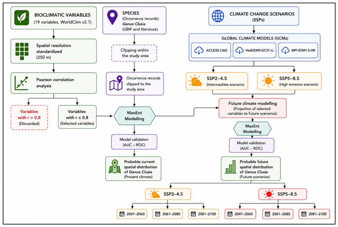
Once the final parameterization was selected, the stability of the prediction was quantified using the 72 bootstrap replicates defined in the modeling process, allowing for an assessment of the variability in the predictions associated with the resampling of the occurrence records [81,99]. Future projections were interpreted as temporal extrapolations of the model rather than as an independent validation, due to the lack of independent future observations against which to directly test the predictions [100,101]. Areas with high, medium, and low dispersion suitability were interpreted as areas of greater multimodel consensus [102,103,104]. Finally, grid cells subject to clamping or environmental extrapolation were identified and interpreted with caution, distinguishing them from projections made within the calibration climate domain [65,81]. The entire methodological process is illustrated in Figure 3.

3. Results

3.1. Statistical Metrics for Model Validation

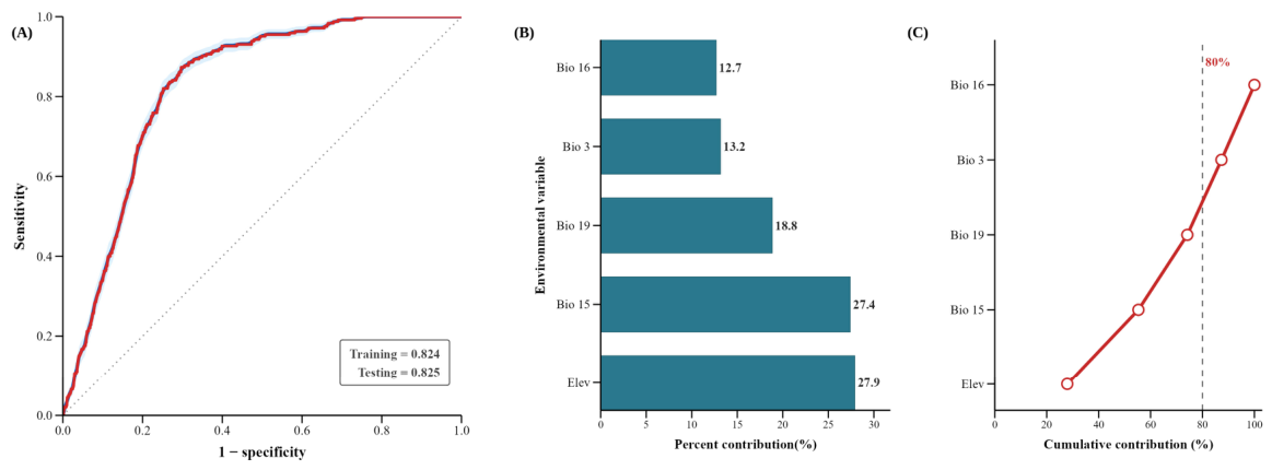
The distribution model for the genus Clusia L. in Peru yielded AUC values of 0.824 for the training dataset and 0.825 for the test dataset, with a minimal difference in performance between the two datasets (Figure 4A). Likewise, the variables with the greatest contribution to the model were elevation (Elev) and precipitation seasonality (Bio 15), with 27.9% and 27.4%, respectively, followed by precipitation during the coldest quarter (Bio 19) at 18.8%, isothermality (Bio 3) at 13.2%, and precipitation during the wettest quarter (Bio 16) at 12.7%, all contributing to the model’s prediction of the spatial distribution of habitats potentially favorable for the genus under study (Figure 4B). The variables Elev, Bio 15, Bio 19, and Bio 3 accounted for more than 80% of the model’s total contribution (Figure 4C), representing the most significant factors in estimating the spatial distribution of Clusia L. habitats in Peru.

3.2. Evaluation of the Model’s Behavior and Performance Stability

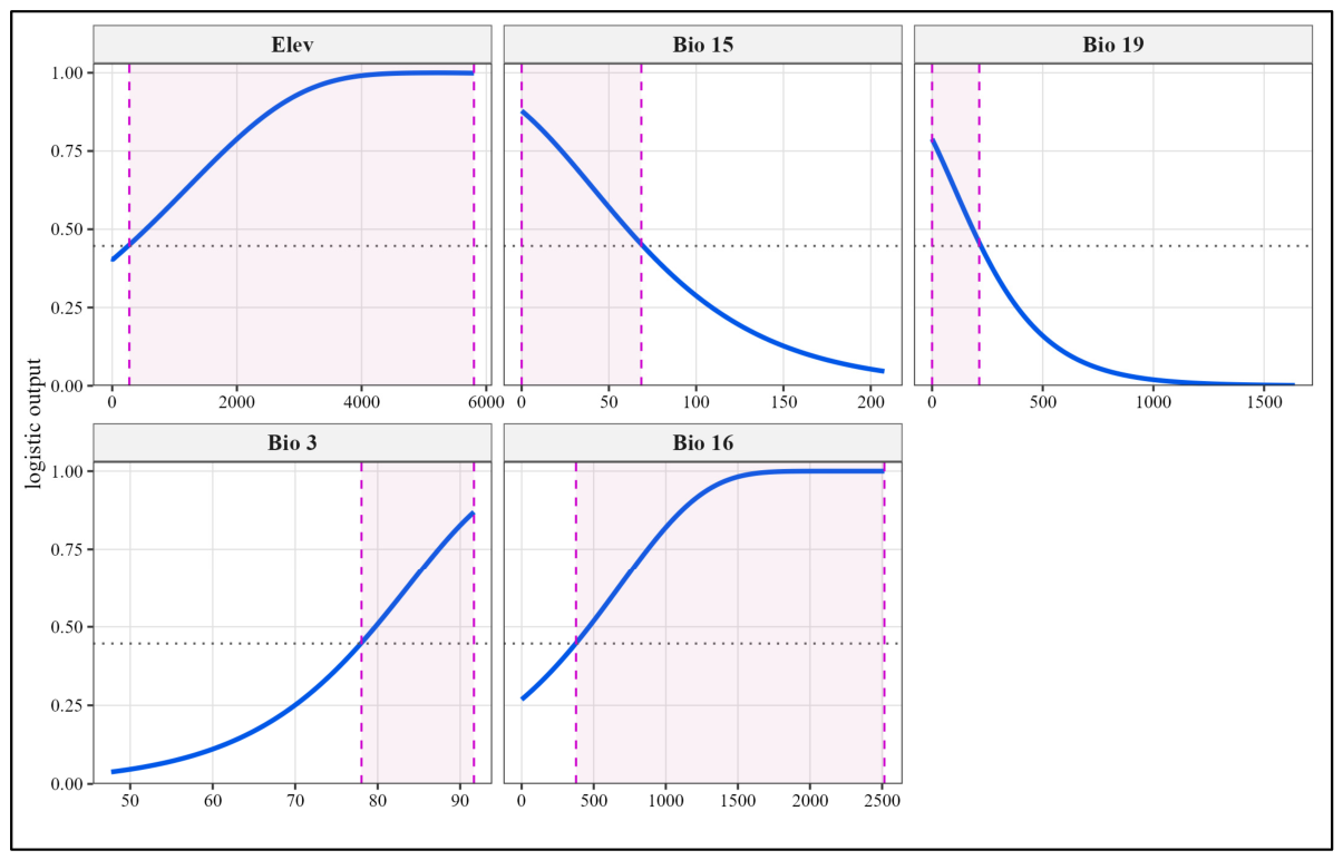
The response curves for the variables used in the modeling (Figure 5) show distinct patterns in habitat suitability for Clusia L. Elevation shows a continuous increase, exceeding the suitability threshold (probability > 0.45) starting at 300 m above sea level and reaching optimal values (~1.00) starting at 4000 m above sea level, indicating a preference for higher-elevation sites. On the other hand, the variables for precipitation seasonality (Bio 15) and precipitation in the coldest quarter (Bio 19) showed a decreasing trend in suitability. For Bio 15, suitability decreased when seasonality exceeded a value of approximately 68%, while for Bio 19, a reduction was observed when precipitation exceeded approximately 210 mm. Meanwhile, isothermality (Bio 3) and precipitation during the wettest quarter (Bio 16) exhibit positive sigmoid responses, with suitability increasing sharply when these values exceed 78% and 380 mm, respectively, and reaching maximum probability (>0.90) at values above 90% and 1500 mm. Thus, it is shown that the presence of the genus in Peru is limited to conditions of high altitude, thermal stability, and high precipitation during the wettest season, combined with low annual rainfall variability.

3.3. Current and Future Potential Distribution of Clusia L.

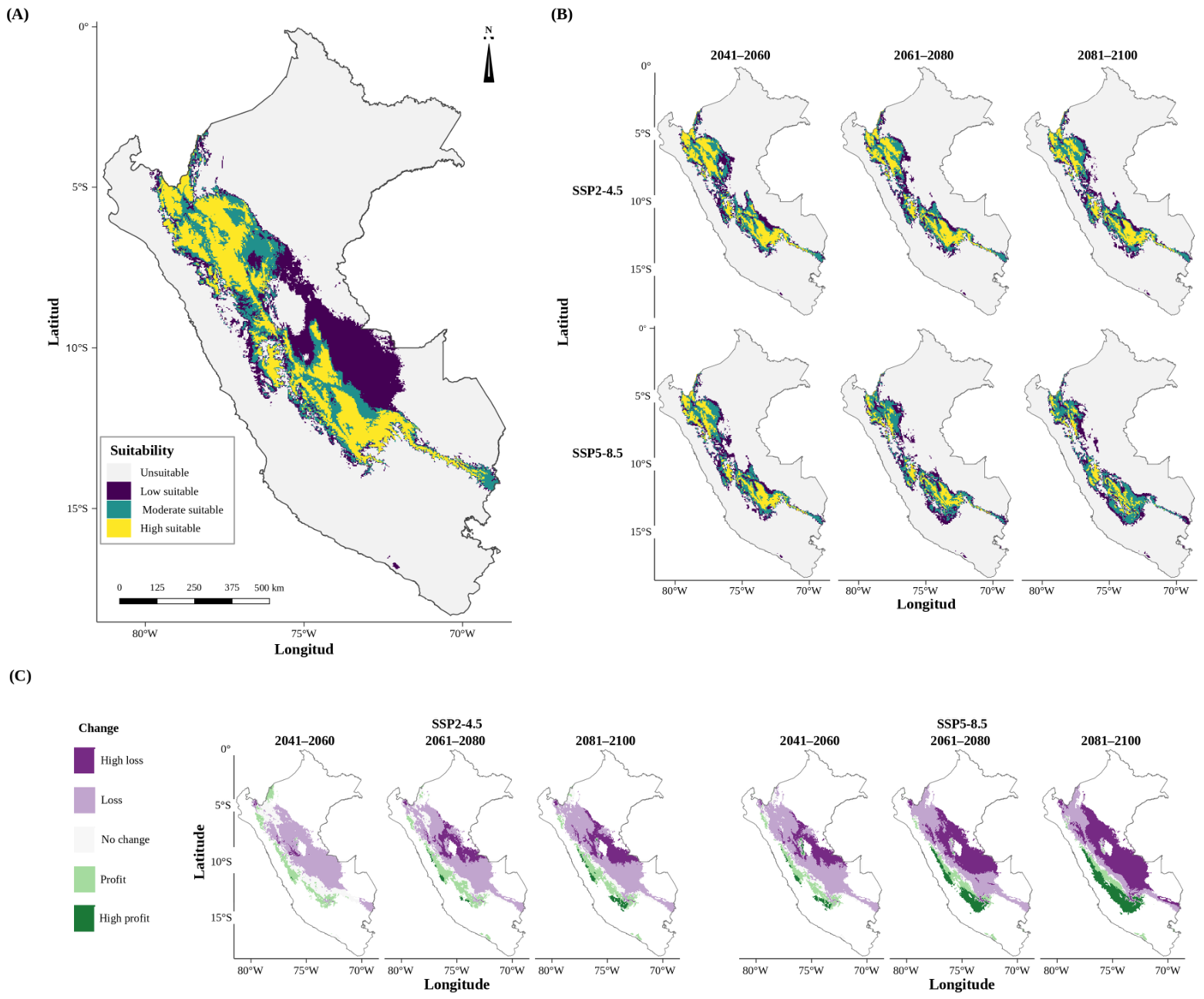
Table 2 shows the current distribution of areas based on their suitability for the presence of Clusia L. in Peru (Table S1). The results indicate that areas with low suitability covered 121,215.61 km2 (9.42%), while the medium- and high-suitability categories accounted for 97,136.43 km2 (7.55%) and 116,645.20 km2 (9.06%), respectively; thus, the areas classified as having medium and high suitability totaled 213,781.63 km2, representing 16.61% of Peruvian territory. The spatial assessment of suitable habitats for Clusia L. shows a concentration in the Andean region of Peru (Figure 6A). The areas identified as having high suitability were distributed discontinuously along the western slope and the inter-Andean valleys; thus, the high and moderate suitability categories indicate greater spatial fragmentation, representing only 16.61% of the evaluated area.
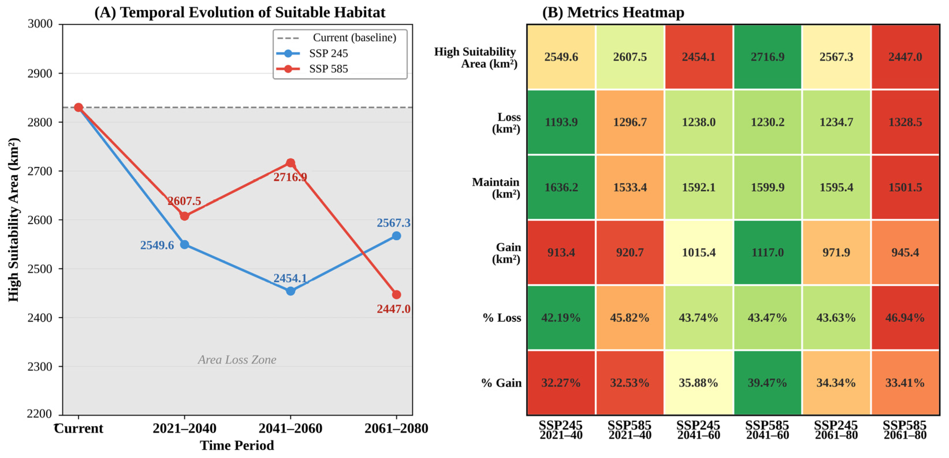
Table 3 shows the quantification of areas by evaluated climate scenario (disaggregated by individual GCM in Table S2); in the SSP2-4.5 scenario, the area classified as highly suitable decreased from 9.68 million ha (7.53%) in 2041–2060 to 7.66 million ha (5.95%) in 2081–2100. Meanwhile, the area classified as having moderate suitability showed a smaller change, decreasing from 9.14 million ha (7.11%) to 8.93 million ha (6.94%) (Figure 7). Thus, these changes indicate a gradual reduction in the most favorable climatic conditions, while areas classified as unsuitable progressively increased their share until they exceeded 82% of the national territory. The SSP5-8.5 scenario showed a more pronounced response. High suitability decreased from 7.37 million ha (5.73%) in 2041–2060 to 4.89 million ha (3.81%) in 2081–2100, representing a loss of approximately 2.48 million ha. Although the average suitability remained close to 7%, the unsuitable area reached 107.74 million ha (83.72%) by the end of the century.
Figure 6B shows the model projections, which indicate a general trend toward a reduction in areas with the greatest climatic suitability for Clusia L. during the future periods evaluated; specifically, in the SSP5-8.5, the decline is more pronounced, as this trend was accompanied by an increase in areas classified as unsuitable, especially toward the end of the century, when the reduction was concentrated primarily in the areas of highest suitability in the northern and central Andes, where a progressively more fragmented distribution was observed, particularly under SSP5-8.5 (individual GCM projections available in Figures S1–S3).
Table 4 shows the quantification of changes in suitability by evaluated climate scenario; in the SSP2-4.5 scenario, the “high loss” category increased dramatically from 0.68 million ha (1.99%) in the 2041–2060 period to 7.06 million ha (20.01%) in 2081–2100. Meanwhile, moderate loss remained the dominant category throughout the entire century, accounting for more than 54% of the area across the three time horizons evaluated. However, areas classified as “no change” decreased from 9.08 million ha (26.29%) to 3.94 million ha (11.18%), while the “gain” and “high gain” categories showed minor increases, collectively reaching 4.84 million ha (13.73%) by the end of the century. These changes indicate that, under SSP2-4.5, continuous habitat degradation predominates, with little compensation from new favorable areas. The SSP5-8.5 scenario showed a considerably more severe response. The area with high loss increased rapidly, rising from 6.63 million ha (18.87%) in 2041–2060 to 19.24 million ha (50.43%) in 2081–2100, meaning that more than half of the assessed area will experience drastic losses in suitability. However, the “high gain” category showed a gradual increase, reaching 5.03 million ha (13.19%) by 2081–2100.
Figure 6C shows the model’s spatiotemporal projections, which indicate a trend toward the retreat and degradation of Clusia L. habitats in Peru. In both scenarios, areas of moderate and high habitat loss are concentrated primarily on the eastern slopes and in the inter-Andean zone of northern and central Peru, exhibiting severe spatial fragmentation. Meanwhile, habitat gains are restricted to higher-altitude areas of the Andean region, a pattern possibly associated with an altitudinal shift in the genus toward higher elevations in response to warming; this process of retreat and degradation of suitable habitat is most severe under the high-emissions scenario SSP5-8.5 (Figure 6).

3.4. Multimodel Uncertainty and Spatial Divergence Among GCMs

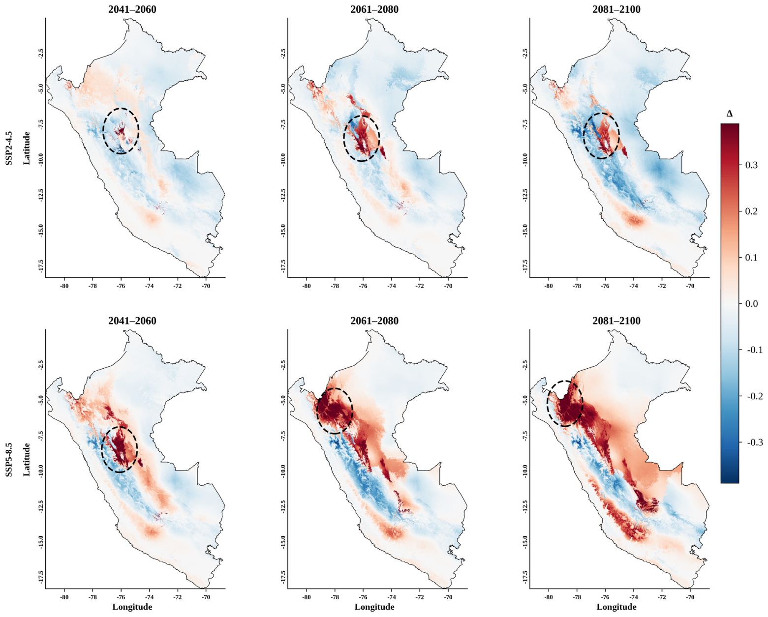
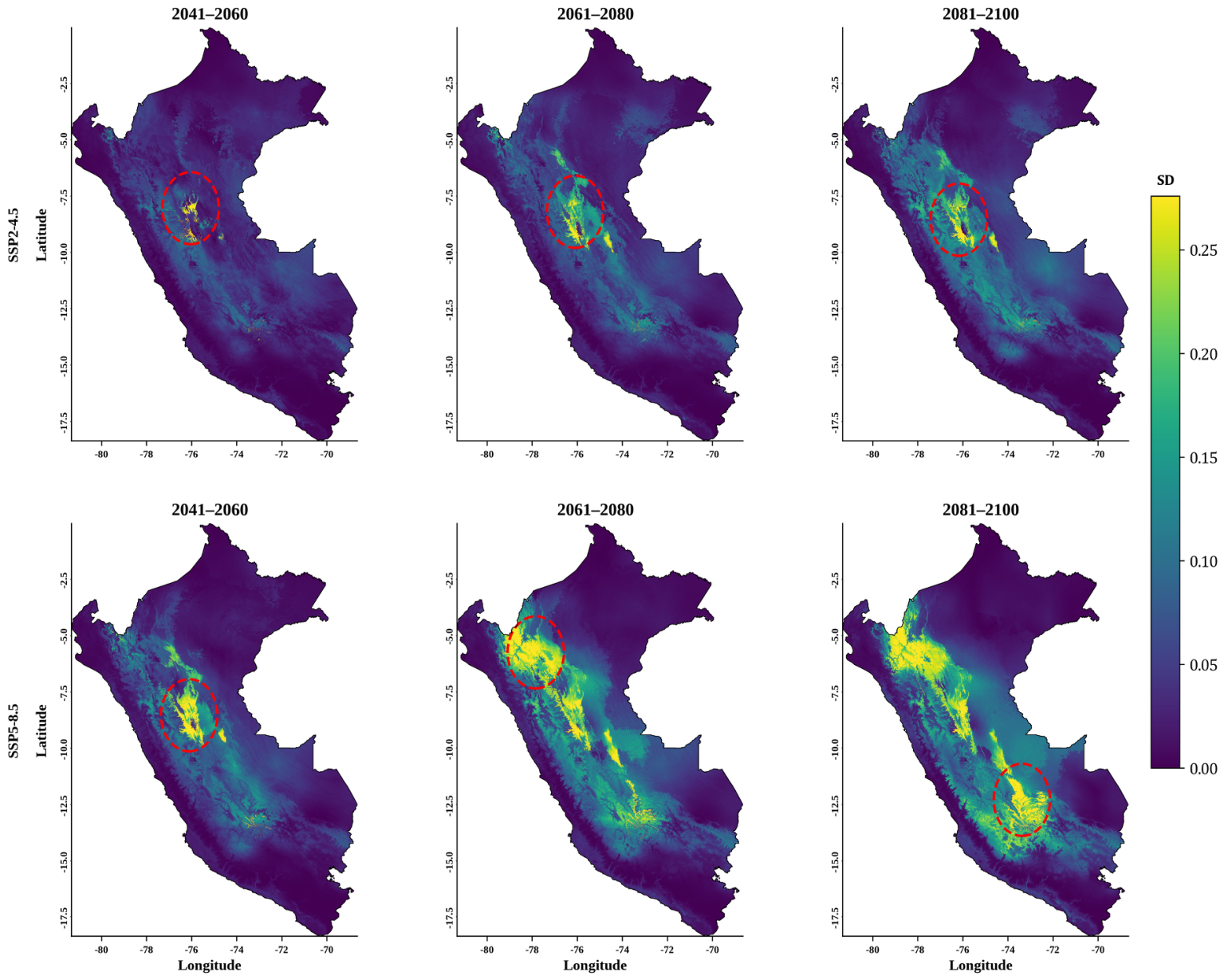
Spatial uncertainty among the three GCMs, measured as the per-cell standard deviation of suitability, was concentrated along the Andean cordillera under both SSP scenarios and increased with time horizon (Figure 8). To further characterize this pattern, HadGEM3-GC31-LL and MPI-ESM1-2-HR were compared directly, as these models generally showed the greatest pairwise divergence. This comparison revealed a consistent spatial asymmetry (Figure 9): divergence was greater and more variable along the western Andean flank (SD = 0.055–0.094 under SSP2-4.5; 0.111–0.168 under SSP5-8.5) than along the eastern, Amazon-facing slopes (SD = 0.040–0.056 under SSP2-4.5; 0.044–0.101 under SSP5-8.5), with the gap between flanks widening progressively toward 2081–2100 and being most pronounced under the high-emission scenario.

4. Discussion

Based on the geospatial modeling conducted in this study, it was found that the territorial suitability for the genus Clusia L. in Peru is concentrated primarily in the Andean region of Peru, based mainly on the seasonality of precipitation. The future projection indicates a trend of progressive contraction of the suitable habitat for Clusia L. in the high-emission SSP scenarios, consistent with the initial hypothesis posed in the study to determine whether changes in future climate trends will generate negative spatial dynamics for species of this genus.
The performance of the MaxEnt model for Clusia L. was evaluated using the ROC curve (AUC), a metric that is not affected by diagnostic thresholds and allows for the evaluation of performance across all possible ranges [104]. The model achieved an AUC of 0.824 for the training set and 0.825 for the test set, values well above the random prediction line (AUC = 0.5) and above the commonly cited threshold of acceptable discrimination (AUC ≥ 0.7) [105], indicating adequate discriminatory performance and a low level of overfitting, attributable to the spatial-block validation method used [106]. Nonetheless, these values are below the range (AUC ≥ 0.9) that other authors consider indicative of excellent model performance [107], and should therefore be interpreted as acceptable rather than exceptional discrimination, consistent with the known limitations of AUC as an absolute accuracy metric [108].
It is important to note that a high statistical discrimination value such as AUC reflects the model’s ability to distinguish presence records from background points within the calibration data, but does not by itself guarantee that the model captures the full ecological requirements of the species or genus. AUC is a relative, correlative measure of statistical fit rather than a validation of ecological mechanism [108]; a model can achieve high discriminatory performance while still reflecting sampling artifacts, a coarse genus-level generalization, or the influence of predictor variables that correlate with, but do not directly cause, suitable conditions for the taxon. Accordingly, the statistical performance reported here should be interpreted as an indicator of internal model consistency rather than as confirmation that the predictors used fully represent the ecological niche of Clusia L.
Geographically, the suitable areas for Clusia L. in Peru are closely linked to the environmental gradient of the Andes mountain range, which is explained primarily by the strong influence of the variables elevation and seasonal precipitation (Bio 15), a pattern consistent with what has been reported for other Andean plant species whose distribution also responds strongly to these same climatic predictors [109]. Furthermore, the response pattern observed for isothermality (Bio 3) suggests that daily and annual thermal stability is a limiting factor for the establishment of Clusia L., consistent with findings for other epiphytic and hemiepiphytic taxa in montane forests, whose survival is severely restricted outside narrow temperature ranges [110]. Taken together, this suggests that the combination of a steep altitudinal gradient and limited thermal tolerance could explain the discontinuous distribution of suitable habitat observed for the genus in Peru [81,111].
In addition to bioclimatic variables, elevation is a determining factor in the territorial suitability of many plant species, as it directly influences their growth, development, and survival [108]. As elevation increases in the mountains, a number of forest site factors such as temperature and soil fertility change, forcing forest species into less favorable habitats, which is reflected in areas with lower species abundance and poorer conditions for adaptability [44]. This was reflected in our model, where elevation (27.9% contribution) played a significant role, confirming that it is a key factor in modeling the suitability of Clusia L., a genus found in Neotropical montane forest sites. This reaffirms that, in Andean forests, variations in tree composition and among populations are closely related to the thermal and altitudinal gradients [45].
The close relationship between Clusia and water regime is best explained by the interaction of Bio 15, Bio 19, and Bio 16 in the model, which confirms that environmental conditions do not act in isolation but rather in combination. These findings have been reported previously by authors such as Brück et al. [112], who found that some Clusia species, such as Clusia flaviflora, respond to water stress, vapor pressure deficit, and soil moisture [112].
The concentration of inter-GCM divergence along the western Andean flank is likely related to structural differences in how HadGEM3-GC31-LL and MPI-ESM1-2-HR represent orographic precipitation and moisture transport across steep topographic gradients. The western slope of the Andes is characterized by a sharp climatic transition from the hyper-arid Pacific coast to montane forest driven by the rain-shadow effect and by ENSO-related sea surface temperature variability, processes that GCMs are known to resolve differently depending on their horizontal resolution and convective parameterization schemes [74,75,76]. In contrast, the eastern, Amazon-facing slopes are climatically more homogeneous and moisture-saturated throughout the year, which likely explains the comparatively higher agreement between models in that region. This is consistent with previous evaluations of CMIP6 model performance in the tropical Andes, which report greater inter-model spread in precipitation-related variables specifically in areas of complex terrain and strong climatic gradients [74,75,76].
This structural source of disagreement has direct implications for the interpretation of our fragmentation results. Because much of the projected high-loss and high-gain area reported in Section 3.3 falls precisely within this zone of greatest inter-model disagreement, the fragmentation patterns described for the western Andean corridor, particularly under SSP5-8.5 by the end of the century, should be interpreted with more caution than those for the eastern, Amazon-facing slopes, where the three GCMs agree more closely.
The importance of the estimated distribution lies in its ability to generate interpretations of Clusia’s future vulnerability. The model estimates that 73.97% of Peruvian territory is unsuitable, while 9.42% is low suitability, 7.55% is medium suitability, and 9.06% is high suitability. This is corroborated by the characteristics of the tropical Andes, where even minimal variations in elevation cause changes in temperature, humidity, and structural changes in vegetation [113]. Taken together, all of this indicates that only 16.61% of Peruvian territory meets high or moderate suitability conditions for species of the genus Clusia L. At this genus-level, regional scale, this provides a coarse framework for flagging broad areas of potential conservation interest for the genus, which would require finer, species-level assessment before informing specific management or land-use interventions.
Furthermore, an analysis of the impact of climate change on the suitability of areas for Clusia L., based on a comparison of the SSP2-4.5 and SSP5-8.5 scenarios, reveals a nonlinear response of the suitable area to the magnitude of radiative forcing, with a gap that progressively widens toward the end of the century. Under the SSP2-4.5 scenario, the area of high suitability decreased from 7.53% to 5.95% between 2041 and 2100, while under the SSP5-8.5 scenario, the reduction was from 5.73% to 3.81% over the same period, reaching a high loss rate of 50.43% of the evaluated territory by 2081–2100. This pattern of disproportionate intensification under more severe climate scenarios has been documented in other modeling studies in the tropical Andes, where the magnitude of suitable area loss increases by a factor of 1.3 to 1.6 when moving from a low-emissions scenario to a high-emissions scenario [114]. Similarly, in Peruvian coastal ecosystems, a progressive increase in the loss of suitable habitat has been reported as the assessed climate scenario intensifies [115], which suggests that this nonlinear sensitivity to the magnitude of radiative forcing could be a recurring pattern in South American flora in response to climate change.
The restriction of fitness gains to higher-elevation areas suggests a process of altitudinal upward shift as a response of the genus to warming, a pattern widely documented in montane forests of the tropical Andes, where tree communities have shown directional changes in their composition toward a greater presence of species originating from lower, warmer elevations as warming progresses [113]. However, this response mechanism faces an obvious physical limitation: the available area gradually decreases as altitude increases, due to the characteristic conical shape of mountain systems, which could create an ecological ceiling for the genus’s expansion [116]. The coexistence of losses concentrated on the eastern slope and limited gains in elevation supports the hypothesis of a redistribution rather than a net expansion of suitable habitat, a pattern consistent with the general principle that climate change shifts species’ distribution limits: contraction at the extreme where conditions are no longer tolerable and gain at the opposite extreme, rather than leading to an expansion of the total occupied area [117], a pattern that remained consistent across the three climate models evaluated (Figures S1–S3).
A key limitation of this study is the uneven botanical sampling coverage of Peru, which may not fully represent the true distribution of the genus Clusia L.; substantial areas, particularly in the lowland Amazon, likely remain under-collected relative to more accessible Andean regions. Although a bias-surface correction based on occurrence density was applied when selecting background points (Section 2.2), this approach mitigates rather than eliminates the influence of geographically uneven sampling effort, and cannot fully distinguish a genuine ecological limit from a collection artifact. This caveat is particularly relevant for interpreting the elevation response curve (Section 3.2), and should be kept in mind when interpreting the spatial patterns reported here. Although the resulting model demonstrates good predictive performance, it is important to note that it represents a generalization of the climatic conditions associated with territorial suitability for Clusia L., and therefore does not capture possible differences in ecological requirements among individual species within the genus. Furthermore, since MaxEnt is an algorithm that works only with presence data, the AUC values obtained should be interpreted as a relative measure of discrimination and not as an absolute estimate of accuracy [118]. The future projections were not subjected to independent validation, since there are no subsequent observations available against which to compare them; consequently, these results should be interpreted as plausible scenarios rather than deterministic predictions. The cells identified through clamping and extrapolation analysis, which are concentrated primarily in the areas of greatest projected change, require cautious interpretation, as they lie outside the calibration climate domain.
We also note that the bias-surface correction applied during background point selection (Section 2.2) was derived solely from the spatial density of the occurrence records themselves, rather than from an independent proxy of sampling effort (e.g., road density or protected-area coverage). This target-group background approach can partially mitigate collection bias, but may also reinforce it if climatically suitable, under-sampled regions are not adequately weighted relative to more accessible, heavily collected areas. We were unable to cross-validate the bias surface against an independent sampling-effort covariate with the current dataset, and we flag this as a methodological limitation for future studies to address.
Beyond the species distribution modelling literature, methodological parallels can also be drawn from remote-sensing-based habitat delineation approaches in topographically complex terrain. For example, long-term Landsat time-series analyses of surface water dynamics in wetlands and waterbodies have demonstrated how fine-scale (30 m) spatial resolution and multi-decadal validation can improve the detection of habitat boundary changes under shifting environmental conditions [119]. While our approach relies on climatic niche modelling rather than direct surface reflectance monitoring, such remote-sensing time-series frameworks offer a complementary perspective on how habitat boundaries can be tracked and validated at high spatial resolution, and may inform future refinements of the spatial validation strategy for genus-level suitability projections such as ours.

5. Conclusions

This study provides the first nationwide assessment of the current and future potential distribution of the genus Clusia L. in Peru. The MaxEnt model, calibrated with spatial block cross-validation, showed acceptable and stable predictive performance (training AUC = 0.824, test AUC = 0.825), with minimal overfitting. Elevation and precipitation seasonality (Bio15) were the strongest predictors, together with precipitation of the coldest quarter (Bio19) and isothermality (Bio3), jointly accounting for over 80% of the model’s contribution, indicating that the genus’s distribution in Peru is governed primarily by the altitudinal gradient of the Andes and by thermal and hydric stability rather than by annual temperature or rainfall totals alone. Suitable habitat (medium and high combined) currently covers only 16.61% of Peruvian territory, distributed discontinuously along the western Andean slope and the inter-Andean valleys.
Climate projections for the SSP2-4.5 and SSP5-8.5 scenarios both indicate a progressive contraction and increasing fragmentation of suitable habitat toward the end of the century, with the high-emissions scenario producing markedly more severe losses (high-loss area reaching 50.43% of the evaluated territory by 2081–2100). Habitat gains were restricted to higher-elevation areas, consistent with an altitudinal range shift rather than a net expansion, and are ultimately constrained by the decreasing land area available at higher elevations. As these future suitability estimates rely on the spatial transfer of a model calibrated under current conditions to climatic conditions projected decades ahead, without independent observations for validation, the percentage changes reported here should be read as plausible relative trends rather than precise quantitative forecasts. These findings offer a coarse-scale spatial baseline that identifies broad regions of climatic vulnerability for Clusia L. in the Peruvian Andes, useful as a starting hypothesis for conservation attention and future monitoring, but not as a substitute for species-level, field-validated assessments when informing site-specific land-use or management decisions. Because the model represents a genus-level generalization and MaxEnt outputs are a relative measure of discrimination rather than an absolute estimate of accuracy, future work should refine these projections at the species level and incorporate independent validation as new occurrence data become available.

Supplementary Materials

The following supporting information can be downloaded at https://www.mdpi.com/article/10.3390/f17091126/s1: Table S1: Area by suitability class under historical climate conditions; Table S2: Area by suitability class projected for each Global Climate Model (GCM), under the SSP2-4.5 and SSP5-8.5 scenarios; Table S3: Area by suitability class of the multi-GCM ensemble, under the SSP2-4.5 and SSP5-8.5 scenarios; Table S4: Jenks natural-breaks thresholds used to classify the habitat suitability change layer (future minus current suitability) into five categories, for each SSP scenario and future period; Table S5: Taxonomic composition of the 245 occurrence records used to calibrate the MaxEnt model for Clusia L. in Peru, by taxon and by life-form group; Figure S1: Spatial distribution of projected climatic suitability for Clusia L. for the period 2041–2060, for each GCM and SSP scenario; Figure S2: idem for 2061–2080; Figure S3: idem for 2081–2100.

Author Contributions

Conceptualization, D.C.-T., J.J.V.-V., J.I.P.-M., N.V.-Y., J.O.R.-A., S.V.V.-R., C.C.-A. and A.J.V.; methodology, D.C.-T., J.J.V.-V., J.I.P.-M., N.V.-Y., J.O.R.-A., S.V.V.-R., C.C.-A. and A.J.V.; software, D.C.-T., S.V.V.-R. and A.J.V.; formal analysis, D.C.-T., S.V.V.-R. and A.J.V.; investigation, D.C.-T., J.J.V.-V., J.I.P.-M., N.V.-Y., J.O.R.-A., S.V.V.-R., C.C.-A. and A.J.V.; resources, A.J.V.; data curation, D.C.-T., S.V.V.-R. and A.J.V.; writing—original draft preparation, D.C.-T., J.J.V.-V., J.I.P.-M., N.V.-Y., J.O.R.-A., S.V.V.-R., C.C.-A. and A.J.V.; writing—review and editing, A.J.V. and S.V.V.-R.; visualization, D.C.-T., J.J.V.-V., J.I.P.-M., N.V.-Y., J.O.R.-A. and S.V.V.-R.; supervision, A.J.V.; project administration, A.J.V. and S.C.-G.; funding acquisition, A.J.V. and S.C.-G. All authors have read and agreed to the published version of the manuscript.

Funding

This research was funded by project “Mejoramiento del servicio de formación de pre grado en educación superior universitaria de la Escuela Profesional de Ingeniería Forestal de la UNTRM Distrito De Chachapoyas—Provincia De Chachapoyas—Departamento De Amazonas”, of the Peruvian Government, with the grant number CUI 2513702. Additionally, the APC was funded by the Vicerrectorado de Investigación, Universidad Nacional Toribio Rodríguez de Mendoza de Amazonas.

Data Availability Statement

Dataset available upon request to the authors.

Acknowledgments

The authors thank the Laboratorio de Analisis Geoespacial y Manejo Forestal (GEOFOREST) of the UNTRM for allowing the development of this research in its facilities and equipment.

Conflicts of Interest

The authors declare no conflicts of interest.

References

  1. Schipper, A.; Hielkema, W.; Ziemba, A. Impact of Climate Change on Biodiversity and Implications for Nature-Based Solutions. Climate 2024, 12, 179. [Google Scholar] [CrossRef] [Scilit]
  2. Calvin, K.; Dasgupta, D.; Krinner, G.; Mukherji, A.; Thorne, P.; Trisos, C.; Romero, J.; Aldunce, P.; Barrett, K.; Blanco, G.; et al. Climate Change 2023: Synthesis Report. 2023. Available online: https://www.ipcc.ch/report/ar6/syr/ (accessed on 10 July 2026).
  3. Ye, C.; Wang, H.; Jin, X. Sharp Increase of Extinction Risk of Mountain Biodiversity under Global Climate Change: Insights from Highly Dispersible Orchids. Biol. Conserv. 2025, 310, 111346. [Google Scholar] [CrossRef] [Scilit]
  4. Ali, M.; Huang, Z.; Wani, Z.; Song, J.; Wu, B.; Hussain, K.; Abdul, R.; Wang, J.; Fang, Z.; Bussmann, R.; et al. Conservation Deficits and Climate-Driven Habitat Shifts of Threatened Plants in South Asia. Geogr. Sustain. 2026, 7, 100477. [Google Scholar] [CrossRef] [Scilit]
  5. Solakis, A.; Hidalgo, N.; Boynton, R.; Thorne, J. Phenological Shifts Since 1830 in 29 Native Plant Species of California and Their Responses to Historical Climate Change. Plants 2025, 14, 843. [Google Scholar] [CrossRef] [Scilit] [PubMed]
  6. Salinas, N.; Cosio, E.; Silman, M.; Meir, P.; Nottingham, A.; Roman, R.; Malhi, Y. Tropical Montane Forests in a Changing Environment. Front. Plant Sci. 2021, 12, 712748. [Google Scholar] [CrossRef] [Scilit] [PubMed]
  7. Ioan, S.; Roseo, F.; Brambilla, M. Mountain Ecosystem Services under a Changing Climate: A Global Perspective. Ecosyst. Serv. 2025, 73, 101732. [Google Scholar] [CrossRef] [Scilit]
  8. Tovar, C.; Carril, A.; Gutiérrez, A.; Ahrends, A.; Fita, L.; Zaninelli, P.; Flombaum, P.; Abarzúa, A.; Alarcón, D.; Aschero, V.; et al. Understanding Climate Change Impacts on Biome and Plant Distributions in the Andes: Challenges and Opportunities. J. Biogeogr. 2022, 49, 1420–1442. [Google Scholar] [CrossRef] [Scilit] [PubMed]
  9. Farfan, W.; Feeley, K.; Myers, J.; Tello, S.; Sallo, J.; Malhi, Y.; Phillips, O.; Baker, T.; Nina, A.; Garcia, K.; et al. Amazonian and Andean Tree Communities Are Not Tracking Current Climate Warming. Proc. Natl. Acad. Sci. USA 2025, 122, e2425619122. [Google Scholar] [CrossRef] [Scilit] [PubMed]
  10. Briscoe, N.; Morris, S.; Mathewson, P.; Buckley, L.; Jusup, M.; Levy, O.; Maclean, I.; Pincebourde, S.; Riddell, E.; Roberts, J.; et al. Mechanistic Forecasts of Species Responses to Climate Change: The Promise of Biophysical Ecology. Glob. Change Biol. 2023, 29, 1451–1470. [Google Scholar] [CrossRef] [Scilit] [PubMed]
  11. Luján, M.; Leverett, A.; Winter, K. Forty Years of Research into Crassulacean Acid Metabolism in the Genus Clusia: Anatomy, Ecophysiology and Evolution. Ann. Bot. 2023, 132, 739–752. [Google Scholar] [CrossRef] [Scilit] [PubMed]
  12. Pachon, P.; Winter, K.; Lasso, E. Updating the Occurrence of Crassulacean Acid Metabolism (CAM) in the Genus Clusia through Carbon Isotope Analysis of Species from Colombia. Photosynthetica 2022, 60, 304–322. [Google Scholar] [CrossRef] [Scilit] [PubMed]
  13. Pietroluongo, M.; Anholeti, M.; Fuly, A.; Valverde, A.; De Paiva, S. Biological Activities of Species of the Genus Clusia L (Clusiaceae): A General Approach. An. Acad. Bras. Ciênc. 2024, 96, e20220649. [Google Scholar] [CrossRef] [Scilit] [PubMed]
  14. Luján, M. Clusia Chuj (Clusiaceae), a New Tree Species from the Border between Guatemala and Mexico. Kew Bull. 2023, 78, 533–537. [Google Scholar] [CrossRef] [Scilit]
  15. Aranda, J.; Campos, E.; Sumich, J.; Virgo, A.; García, M.; Winter, K.; Luján, M.; Hammel, B. Tidying up the Small-Leaved Clusia Taxonomy: Description of Clusia Nanophylla (Clusiaceae), a New Tree Species from Panama and Comments on Its Previously Used Names. Kew Bull. 2025, 80, 975–981. [Google Scholar] [CrossRef] [Scilit]
  16. Wodcke, E.; Luján, M.; Hammel, B. Clusia Salicifolia (Clusiaceae), a New Hemiepiphyte Species from Costa Rica and Panama. Kew Bull. 2024, 79, 185–190. [Google Scholar] [CrossRef] [Scilit]
  17. Luján, M.; Paolini, J.; Sanoja, E.; Rojas, C.A.; Ely, F. Integrative Taxonomy Led to Recognising Clusia Reginae (Clusiaceae), a New Tree Species from the Venezuelan Andes. Kew Bull. 2024, 79, 191–200. [Google Scholar] [CrossRef] [Scilit]
  18. GBIF Registros Biológicos. Available online: https://www.gbif.org/es/occurrence/search?occurrenceStatus=PRESENT&taxonKey=3R8S&country=PE (accessed on 10 July 2026).
  19. Moudrý, V.; Bazzichetto, M.; Remelgado, R.; Devillers, R.; Lenoir, J.; Mateo, R.; Lembrechts, J.; Sillero, N.; Lecours, V.; Cord, A.; et al. Optimising Occurrence Data in Species Distribution Models: Sample Size, Positional Uncertainty, and Sampling Bias Matter. Ecography 2024, 2024, e07294. [Google Scholar] [CrossRef] [Scilit]
  20. Daru, B.; Park, D.; Primack, R.; Willis, C.; Barrington, D.; Whitfeld, T.; Seidler, T.; Sweeney, P.W.; Foster, D.; Ellison, A.; et al. Widespread Sampling Biases in Herbaria Revealed from Large-Scale Digitization. New Phytol. 2018, 217, 939–955. [Google Scholar] [CrossRef] [Scilit] [PubMed]
  21. Pimenta, M.; Alaves, A.; Fernando, S.; Pereira, M.; Almeida, R.; Soares, A.; Falcon, G.; Raíces, D.; De Marco, J. One Size Does Not Fit All: Priority Areas for Real World Problems. Ecol. Model. 2022, 470, 110013. [Google Scholar] [CrossRef] [Scilit]
  22. Critchlow, R.; Cunningham, C.; Crick, H.; Macgregor, N.; Morecroft, M.; Pearce, J.; Oliver, T.; Carroll, M.; Beale, C. Multi-Taxa Spatial Conservation Planning Reveals Similar Priorities between Taxa and Improved Protected Area Representation with Climate Change. Biodivers. Conserv. 2022, 31, 683–702. [Google Scholar] [CrossRef] [Scilit]
  23. Qazi, A.; Saqib, Z.; Zaman-ul-Haq, M. Trends in Species Distribution Modelling in Context of Rare and Endemic Plants: A Systematic Review. Ecol. Process. 2022, 11, 40. [Google Scholar] [CrossRef] [Scilit]
  24. Xu, W.; Luo, D.; Peterson, K.; Zhao, Y.; Yu, Y.; Ye, Z.; Sun, J.; Yan, K.; Wang, T. Advancements in Ecological Niche Models for Forest Adaptation to Climate Change: A Comprehensive Review. Biol. Rev. 2025, 100, 1754–1781. [Google Scholar] [CrossRef] [Scilit] [PubMed]
  25. Franklin, J. Species Distribution Modelling Supports the Study of Past, Present and Future Biogeographies. J. Biogeogr. 2023, 50, 1533–1545. [Google Scholar] [CrossRef] [Scilit]
  26. Escamilla, J.; Sedda, L.; Diggle, P.; Atkinson, P. A Joint Distribution Framework to Improve Presence-Only Species Distribution Models by Exploiting Opportunistic Surveys. J. Biogeogr. 2022, 49, 1176–1192. [Google Scholar] [CrossRef] [Scilit]
  27. Leroy, B. Choosing Presence-Only Species Distribution Models. J. Biogeogr. 2023, 50, 247–250. [Google Scholar] [CrossRef] [Scilit]
  28. Nolan, V.; Gilbert, F.; Reader, T. Solving Sampling Bias Problems in Presence–Absence or Presence-Only Species Data Using Zero-Inflated Models. J. Biogeogr. 2022, 49, 215–232. [Google Scholar] [CrossRef] [Scilit]
  29. Barber, R.; Ball, S.; Morris, R.; Gilbert, F. Target-Group Backgrounds Prove Effective at Correcting Sampling Bias in Maxent Models. Divers. Distrib. 2022, 28, 128–141. [Google Scholar] [CrossRef] [Scilit]
  30. Worldclim Datos Climáticos Futuros: Documentación de WorldClim 1. Available online: https://www.worldclim.org/data/cmip6/cmip6climate (accessed on 10 July 2026).
  31. WorldClim Bioclimatic Variables—WorldClim Documentation. Available online: https://www.worldclim.org/data/bioclim (accessed on 10 July 2026).
  32. Fick, S.; Hijmans, R. WorldClim 2: New 1-Km Spatial Resolution Climate Surfaces for Global Land Areas. Int. J. Climatol. 2017, 37, 4302–4315. [Google Scholar] [CrossRef] [Scilit]
  33. Sparey, M.; Cox, P.; Williamson, M. Bioclimatic Change as a Function of Global Warming from CMIP6 Climate Projections. Biogeosciences 2023, 20, 451–488. [Google Scholar] [CrossRef] [Scilit]
  34. Intergovernmental Panel on Climate Change. Future Global Climate: Scenario-Based Projections and Near-Term Information Supplementary Material; Cambridge University Press: Cambridge, UK, 2021. [Google Scholar]
  35. Rojas, N.; García, L.; Cotrina, A.; Goñas, M.; Salas, R.; Silva, J.; Oliva, M. Land Suitability for Cocoa Cultivation in Peru: AHP and MaxEnt Modeling in a GIS Environment. Agronomy 2022, 12, 2930. [Google Scholar] [CrossRef] [Scilit]
  36. Santos, V.; Macedo, J. Modelización de La Distribución Potencial de Gentianella Weberbaueri (Gentianaceae) En Perú. Lilloa 2025, 62, 747–761. [Google Scholar] [CrossRef] [Scilit] [PubMed]
  37. Cubas, J.; Chuquibala, B.; Atalaya, N.; Tineo, D.; Taboada, V.; Cabrera, H.; Cruz, J.; Goñas, M.; Gómez, D. Modeling the Potential Distribution of Musa (AAB), Cv. ‘Bellaco’ and Carica Papaya under Climate Change Scenarios in the Provinces of Jaén and San Ignacio. Smart Agric. Technol. 2026, 14, 102271. [Google Scholar] [CrossRef] [Scilit]
  38. Vergara, A.; Cieza, D.; Ocaña, C.; Quiñonez, L.; Idrogo, G.; Muñoz, L.; Auquiñivin, E.; Cruzalegui, R.; Arbizu, C. Current and Future Spatial Distribution of the Genus Cinchona in Peru: Opportunities for Conservation in the Face of Climate Change. Sustainability 2023, 15, 14109. [Google Scholar] [CrossRef] [Scilit]
  39. Zevallos, J.; Lavado-Casimiro, W. Climate Change Impact on Peruvian Biomes. Forests 2022, 13, 238. [Google Scholar] [CrossRef] [Scilit]
  40. Guzman, B.; Cotrina, A.; Allauja, E.; Olivera, C.; Ramos, J.; Hoyos, M.; Barboza, E.; Torres, C.; Oliva, M. Predicting Potential Distribution and Identifying Priority Areas for Conservation of the Yellow-Tailed Woolly Monkey (Lagothrix Flavicauda) in Peru. J. Nat. Conserv. 2022, 70, 126302. [Google Scholar] [CrossRef] [Scilit]
  41. Ministerio del Ambiente [MINAM]. Definiciones Conceptuales de los Ecosistemas del Perú. 2022. Available online: https://sinia.minam.gob.pe/sites/default/files/archivos/public/docs/5.%20Definiciones-Conceptuales-de-los-Ecosistemas_MINAM.pdf (accessed on 6 August 2026).
  42. Ministerio del Ambiente [MINAM]. Mapa Nacional de Ecosistemas del Perú. 2023. Available online: https://sinia.minam.gob.pe/sites/default/files/archivos/public/docs/1.%20Mapa%20Nacional%20de%20Ecosistemas%20del%20Per%C3%BA.pdf (accessed on 6 August 2026).
  43. Quinteros, Y.; Macedo, J.; Santos, V.; Angeles, F.; Gómez, D.; Campos, J.; Solis, J.; Salinas, A.; Valencia, Z. Floristic Diversity and Distribution Pattern along an Altitudinal Gradient in the Central Andes: A Case Study of Cajatambo, Peru. Plants 2024, 13, 3328. [Google Scholar] [CrossRef] [Scilit] [PubMed]
  44. Guerrero, A.; Rodríguez, E.; Leiva, S.; Pollack, L. Zonas de Vida En El Proceso de La Zonificación Ecológica Económica (ZEE) de La Provincia de Trujillo, Región La Libertad, Perú. Arnaldoa 2019, 26, 761–792. [Google Scholar]
  45. Holzmann, K.L. Exploring Biodiversity from Andean Peaks to the Amazonian Lowland. Bull. Ecol. Soc. Am. 2025, 106, e70013. [Google Scholar] [CrossRef] [Scilit]
  46. Martinez, G.; Rojas, C.; Delgado, G.; Zune, F.; Huaman, A.; Murillo, Y.; Brightsmith, D. Floristic composition and diversity in four amazon rainforest habitats from Tambopata, Madre de Dios, Peru. Folia Amaz. 2023, 32, e32687. [Google Scholar] [CrossRef] [Scilit]
  47. Reyes, C.; Reynel, C.; Palacios, S.; Huamani, J. Plant communities determined by climate and soil parameters along an altitudinal gradient in the Chanchamayo valley, Peru. Folia Amaz. 2024, 33, e33776. [Google Scholar] [CrossRef] [Scilit]
  48. Urquiaga, E.; Bader, M.; Kessler, M. Contrasting Topography-Vegetation Relationships at Natural and Human-Influenced Mountain Treelines in the Peruvian Andes. Landsc. Ecol. 2024, 39, 213. [Google Scholar] [CrossRef] [Scilit]
  49. Jury, M.; Alfaro, L. Peruvian North Coast Climate Variability and Regional Ocean–Atmosphere Forcing. Coasts 2024, 4, 508–534. [Google Scholar] [CrossRef] [Scilit]
  50. Newell, F.; Ausprey, I.; Robinson, S. Spatiotemporal Climate Variability in the Andes of Northern Peru: Evaluation of Gridded Datasets to Describe Cloud Forest Microclimate and Local Rainfall. Int. J. Climatol. 2022, 42, 5892–5915. [Google Scholar] [CrossRef] [Scilit]
  51. Sulca, S.; Calle, V.; Acuña, D. Ocean-atmospheric macro-scale pattern associated with extreme droughts in the southern highlands of Peru. Ecol. Apl. 2022, 21, 57–66. [Google Scholar]
  52. de Melo, P.H.A.; Bystriakova, N.; Lucas, E.; Monro, A.K. A New R Package to Parse Plant Species Occurrence Records into Unique Collection Events Efficiently Reduces Data Redundancy. Sci. Rep. 2024, 14, 5450. [Google Scholar] [CrossRef] [Scilit] [PubMed]
  53. Nusch, C.J.; Cagnina, L.C.; Peloche, S.B.; Villarreal, G.L.; Lira, A.J.; Antonelli, R.L.; Folegotto, L.E.; Errecalde, M.L.; De Giusti, M.R. Clasificación Automática de Materias En Repositorios Institucionales Mediante Aprendizaje Supervisado y Representaciones Vectoriales Multilingües: Un Estudio de Caso En SEDICI. In Proceedings of the XIV Conferencia Internacional BIREDIAL-ISTEC, Brasilia, Brazil, 8–10 October 2025. [Google Scholar] [CrossRef] [Scilit]
  54. Li, Y.; Zhang, T.; Zhou, H.; Wang, B.; Xu, P.; Sun, H.; Xia, F.; Shao, W. Climatic Suitability of Cornus Officinalis Across Paleoclimatic, Current, and Future Climates: Implications for Conservation and Climate-Informed Cultivation. Horticulturae 2026, 12, 989. [Google Scholar] [CrossRef] [Scilit]
  55. Driouech, H.; El Haddouti, I.; Alaoui Mhamdi, O.; Hafid, A.; Louahlia, S.; Benfodda, Z.; Libiad, M.; Khabbach, A. Predicting the Potential Distribution of Stachys Fontqueri Pau (Lamiaceae), a Strictly Endemic Medicinal Species of the Moroccan Rif, Under the Effects of Climate Change for Sustainable Conservation. Sustainability 2026, 18, 8279. [Google Scholar] [CrossRef] [Scilit]
  56. Zizka, A.; Silvestro, D.; Andermann, T.; Azevedo, J.; Duarte Ritter, C.; Edler, D.; Farooq, H.; Herdean, A.; Ariza, M.; Scharn, R.; et al. CoordinateCleaner: Standardized Cleaning of Occurrence Records from Biological Collection Databases. Methods Ecol. Evol. 2019, 10, 744–751. [Google Scholar] [CrossRef] [Scilit]
  57. Ribeiro, B.R.; Velazco, S.J.E.; Guidoni-Martins, K.; Tessarolo, G.; Jardim, L.; Bachman, S.P.; Loyola, R. Bdc: A Toolkit for Standardizing, Integrating and Cleaning Biodiversity Data. Methods Ecol. Evol. 2022, 13, 1421–1428. [Google Scholar] [CrossRef] [Scilit]
  58. Gábor, L.; Moudrý, V.; Lecours, V.; Malavasi, M.; Barták, V.; Fogl, M.; Šímová, P.; Rocchini, D.; Václavík, T. The Effect of Positional Error on Fine Scale Species Distribution Models Increases for Specialist Species. Ecography 2020, 43, 256–269. [Google Scholar] [CrossRef] [Scilit]
  59. Caballero, L.; Fajardo, F.; Calbi, M.; Silva, G. Climate Change Can Drive a Significant Loss of Suitable Habitat for Polylepis Quadrijuga, a Treeline Species in the Sky Islands of the Northern Andes. Front. Ecol. Evol. 2021, 9, 661550. [Google Scholar] [CrossRef] [Scilit]
  60. Amiri, M.; Tarkesh, M.; Jafari, R.; Jetschke, G. Bioclimatic Variables from Precipitation and Temperature Records vs. Remote Sensing-Based Bioclimatic Variables: Which Side Can Perform Better in Species Distribution Modeling? Ecol. Inform. 2020, 57, 101060. [Google Scholar] [CrossRef] [Scilit]
  61. Poggio, L.; Simonetti, E.; Gimona, A. Enhancing the WorldClim Data Set for National and Regional Applications. Sci. Total Environ. 2018, 625, 1628–1643. [Google Scholar] [CrossRef] [Scilit] [PubMed]
  62. Merkenschlager, C.; Bangelesa, F.; Paeth, H.; Hertig, E. Blessing and Curse of Bioclimatic Variables: A Comparison of Different Calculation Schemes and Datasets for Species Distribution Modeling within the Extended Mediterranean Area. Ecol. Evol. 2023, 13, e10553. [Google Scholar] [CrossRef] [Scilit] [PubMed]
  63. Maharjan, S.K.; Sterck, F.J.; Raes, N.; Poorter, L. Temperature and Soils Predict the Distribution of Plant Species along the Himalayan Elevational Gradient. J. Trop. Ecol. 2022, 38, 58–70. [Google Scholar] [CrossRef] [Scilit]
  64. Biella, P.; Cornalba, M.; Rasmont, P.; Neumayer, J.; Mei, M.; Brambilla, M. Climate Tracking by Mountain Bumblebees across a Century: Distribution Retreats, Small Refugia and Elevational Shifts. Glob. Ecol. Conserv. 2024, 54, e03163. [Google Scholar] [CrossRef] [Scilit]
  65. Soley-Guardia, M.; Alvarado-Serrano, D.F.; Anderson, R.P. Top Ten Hazards to Avoid When Modeling Species Distributions: A Didactic Guide of Assumptions, Problems, and Recommendations. Ecography 2024, 2024, e06852. [Google Scholar] [CrossRef] [Scilit]
  66. Bongiovanni, G.; Matiu, M.; Crespi, A.; Napoli, A.; Majone, B.; Zardi, D. EEAR-Clim: A High-Density Observational Dataset of Daily Precipitation and Air Temperature for the Extended European Alpine Region. Earth Syst. Sci. Data 2025, 17, 1367–1391. [Google Scholar] [CrossRef] [Scilit]
  67. Vergara, A.J.; Valqui-Reina, S.V.; Gómez-Santillán, Y.; Cieza-Tarrillo, D.; Zúñiga, C.L.-O.; Munoz-Astecker, L.; Whetten, R.; Arbizu, C.I. Current and Future Spatial Dynamics of the Edaphoclimatic Distribution of Ceiba Pentandra in the Geographical Department of Amazonas, Peru. Front. For. Glob. Chang. 2026, 9, 1835040. [Google Scholar] [CrossRef] [Scilit]
  68. Cushman, S.A.; Kaszta, Z.M.; Burns, P.; Hakkenberg, C.R.; Jantz, P.; Macdonald, D.W.; Brodie, J.F.; Deith, M.C.M.; Goetz, S. Simulating Multi-Scale Optimization and Variable Selection in Species Distribution Modeling. Ecol. Inform. 2024, 83, 102832. [Google Scholar] [CrossRef] [Scilit]
  69. Dormann, C.F.; Elith, J.; Bacher, S.; Buchmann, C.; Carl, G.; Carré, G.; Marquéz, J.R.G.; Gruber, B.; Lafourcade, B.; Leitão, P.J.; et al. Collinearity: A Review of Methods to Deal with It and a Simulation Study Evaluating Their Performance. Ecography 2013, 36, 27–46. [Google Scholar] [CrossRef] [Scilit]
  70. Eyring, V.; Bony, S.; Meehl, G.; Senior, C.; Stevens, B.; Stouffer, R.; Taylor, K. Overview of the Coupled Model Intercomparison Project Phase 6 (CMIP6) Experimental Design and Organization. Geosci. Model Dev. 2016, 9, 1937–1958. [Google Scholar] [CrossRef] [Scilit]
  71. Bi, D.; Dix, M.; Marsland, S.; O’farrell, S.; Sullivan, A.; Bodman, R.; Law, R.; Harman, I.; Srbinovsky, J.; Rashid, H.; et al. Configuration and Spin-up of ACCESS-CM2, the New Generation Australian Community Climate and Earth System Simulator Coupled Model. J. South. Hemisph. Earth Syst. Sci. 2020, 70, 225–251. [Google Scholar] [CrossRef] [Scilit]
  72. O’Neill, B.; Tebaldi, C.; Van Vuuren, D.; Eyring, V.; Friedlingstein, P.; Hurtt, G.; Knutti, R.; Kriegler, E.; Lamarque, J.; Lowe, J.; et al. The Scenario Model Intercomparison Project (ScenarioMIP) for CMIP6. Geosci. Model Dev. 2016, 9, 3461–3482. [Google Scholar] [CrossRef] [Scilit]
  73. Riahi, K.; van Vuuren, D.P.; Kriegler, E.; Edmonds, J.; O’Neill, B.; Fujimori, S.; Bauer, N.; Calvin, K.; Dellink, R.; Fricko, O.; et al. The Shared Socioeconomic Pathways and Their Energy, Land Use, and Greenhouse Gas Emissions Implications: An Overview. Glob. Environ. Chang. 2017, 42, 153–168. [Google Scholar] [CrossRef] [Scilit]
  74. Almazroui, M.; Ashfaq, M.; Islam, M.N.; Rashid, I.U.; Kamil, S.; Abid, M.; O’Brien, E.; Ismail, M.; Reboita, M.; Sörensson, A.A.; et al. Assessment of CMIP6 Performance and Projected Temperature and Precipitation Changes Over South America. Earth Syst. Environ. 2021, 5, 155–183. [Google Scholar] [CrossRef] [Scilit]
  75. Arias, P.; Correa, I.; Fita, L.; Martínez, J.; Alvarez, C.; Alves, L.; Boisier, J.; Campozano, L.; Espinoza, J.; Junquas, C.; et al. How Well CMIP6 Models Simulate Key Boundary Conditions Affecting South American Climate? Insights for Regional Modeling Efforts. Clim. Dyn. 2025, 63, 231. [Google Scholar] [CrossRef] [Scilit]
  76. Fernandez, C.; Hattermann, F.; Krysanova, V.; Vega, F.; Menz, C.; Gleixner, S.; Bronstert, A. High-Resolution Climate Projection Dataset Based on CMIP6 for Peru and Ecuador: BASD-CMIP6-PE. Sci. Data 2024, 11, 34. [Google Scholar] [CrossRef] [Scilit] [PubMed]
  77. Goberville, E.; Beaugrand, G.; Hautekèete, N.; Piquot, Y.; Luczak, C. Uncertainties in the Projection of Species Distributions Related to General Circulation Models. Ecol. Evol. 2015, 5, 1100–1116. [Google Scholar] [CrossRef] [Scilit] [PubMed]
  78. Zhang, L.; Liu, S.; Sun, P.; Wang, T.; Wang, G.; Zhang, X.; Wang, L. Consensus Forecasting of Species Distributions: The Effects of Niche Model Performance and Niche Properties. PLoS ONE 2015, 10, e0120056. [Google Scholar] [CrossRef] [Scilit] [PubMed]
  79. Meinshausen, M.; Nicholls, Z.R.J.; Lewis, J.; Gidden, M.J.; Vogel, E.; Freund, M.; Beyerle, U.; Gessner, C.; Nauels, A.; Bauer, N.; et al. The Shared Socio-Economic Pathway (SSP) Greenhouse Gas Concentrations and Their Extensions to 2500. Geosci. Model Dev. 2020, 13, 3571–3605. [Google Scholar] [CrossRef] [Scilit]
  80. Noce, S.; Caporaso, L.; Santini, M. A New Global Dataset of Bioclimatic Indicators. Sci. Data 2020, 7, 398. [Google Scholar] [CrossRef] [Scilit] [PubMed]
  81. Zurell, D.; Franklin, J.; König, C.; Bouchet, P.; Dormann, C.; Elith, J.; Fandos, G.; Feng, X.; Guillera-Arroita, G.; Guisan, A.; et al. A Standard Protocol for Reporting Species Distribution Models. Ecography 2020, 43, 1261–1277. [Google Scholar] [CrossRef] [Scilit]
  82. Lan, Y.; Wu, X.; Xu, M.; Li, K.; Huan, Y.; Zhou, G.; Lun, F.; Shang, W.; Zhang, R.; Xie, Y. High-Resolution Global Distribution Projections of 10 Rodent Genera under Diverse SSP-RCP Scenarios, 2021–2100. Sci. Data 2025, 12, 1467. [Google Scholar] [CrossRef] [Scilit] [PubMed]
  83. da Silveira, L.C.L.; Marcon, A.K.; Liebsch, D.; Marchioro, C.A. Where the Black-Horned Capuchins Roam: Present and Future Ranges of Sapajus Nigritus and Their Overlap with Pine Plantations. Ecosystems 2026, 29, 59. [Google Scholar] [CrossRef] [Scilit]
  84. Phillips, S.; Aneja, V.; Kang, D.; Arya, S. Modelling and Analysis of the Atmospheric Nitrogen Deposition in North Carolina. Int. J. Glob. Environ. Issues 2006, 6, 231–252. [Google Scholar] [CrossRef] [Scilit]
  85. Zhu, Y.; Hao, Z.; Zhu, L.; Shen, L.; Liu, Y.; Gan, M. Progress in the Application of Machine Learning in the Field of Single-Cell and Spatial Transcriptomics. Genes 2026, 17, 604. [Google Scholar] [CrossRef] [Scilit] [PubMed]
  86. Kass, J.; Muscarella, R.; Galante, P.; Bohl, C.; Pinilla, G.; Boria, R.; Soley, M.; Anderson, R. ENMeval 2.0: Redesigned for Customizable and Reproducible Modeling of Species’ Niches and Distributions. Methods Ecol. Evol. 2021, 12, 1602–1608. [Google Scholar] [CrossRef] [Scilit]
  87. Smith, A.B.; Godsoe, W.; Rodríguez-Sánchez, F.; Wang, H.H.; Warren, D. Niche Estimation Above and Below the Species Level. Trends Ecol. Evol. 2019, 34, 260–273. [Google Scholar] [CrossRef] [Scilit] [PubMed]
  88. López, K.; Osorio, L.; Rojas, O.; Chiappa, X.; Patrón, C.; Yáñez, C. An Exhaustive Evaluation of Modeling Ecological Niches above Species Level to Predict Marine Biological Invasions. Mar. Environ. Res. 2023, 186, 105926. [Google Scholar] [CrossRef] [Scilit] [PubMed]
  89. Fourcade, Y.; Engler, J.O.; Rödder, D.; Secondi, J. Mapping Species Distributions with MAXENT Using a Geographically Biased Sample of Presence Data: A Performance Assessment of Methods for Correcting Sampling Bias. PLoS ONE 2014, 9, e97122. [Google Scholar] [CrossRef] [Scilit] [PubMed]
  90. Wang, Z.; Li, N.; Xu, R.; Ying, Z.; Ruan, X.; Wang, T.; Liao, W.; Su, Y. Distribution Model and Prediction of the Tree Fern Alsophila Costularis Baker (Cyatheaceae) in China. Ecol. Evol. 2024, 14, e11594. [Google Scholar] [CrossRef] [Scilit] [PubMed]
  91. Muscarella, R.; Galante, P.J.; Soley-Guardia, M.; Boria, R.A.; Kass, J.M.; Uriarte, M.; Anderson, R.P. ENMeval: An R Package for Conducting Spatially Independent Evaluations and Estimating Optimal Model Complexity for Maxent Ecological Niche Models. Methods Ecol. Evol. 2014, 5, 1198–1205. [Google Scholar] [CrossRef] [Scilit]
  92. Hirzel, A.H.; Le Lay, G.; Helfer, V.; Randin, C.; Guisan, A. Evaluating the Ability of Habitat Suitability Models to Predict Species Presences. Ecol. Model. 2006, 199, 142–152. [Google Scholar] [CrossRef] [Scilit]
  93. Radosavljevic, A.; Anderson, R.P. Making Better Maxent Models of Species Distributions: Complexity, Overfitting and Evaluation. J. Biogeogr. 2014, 41, 629–643. [Google Scholar] [CrossRef] [Scilit]
  94. Phillips, S.J.; Anderson, R.P.; Dudík, M.; Schapire, R.E.; Blair, M.E. Opening the Black Box: An Open-Source Release of Maxent. Ecography 2017, 40, 887–893. [Google Scholar] [CrossRef] [Scilit]
  95. Li, Y.; Li, M.; Li, C.; Liu, Z. Optimized Maxent Model Predictions of Climate Change Impacts on the Suitable Distribution of Cunninghamia Lanceolata in China. Forests 2020, 11, 302. [Google Scholar] [CrossRef] [Scilit]
  96. Silva, C.; Adams, C.; Paschoaletto, K.; De Barros, M.; Pereira, M.; McAlpine, C. Using Species Distribution Models to Predict Potential Landscape Restoration Effects on Puma Conservation. PLoS ONE 2016, 11, e0145232. [Google Scholar] [CrossRef] [Scilit] [PubMed]
  97. Ren, J.; Li, S.; Zhang, Y.; Yang, Q.; Liu, J.; Fan, J.; Xiang, Y. MaxEnt-Based Evaluation of Climate Change Effects on the Habitat Suitability of Magnolia Officinalis in China. Front. Plant Sci. 2025, 16, 1601585. [Google Scholar] [CrossRef] [Scilit] [PubMed]
  98. Serafini, C.; Cosentino, F.; Amori, G.; Maiorano, L. Modelling Species Distribution at the Boundaries of the Earth’s Climate. Glob. Ecol. Biogeogr. 2025, 34, e70082. [Google Scholar] [CrossRef] [Scilit]
  99. Merow, C.; Smith, M.; Edwards, T.; Guisan, A.; Mcmahon, S.; Normand, S.; Thuiller, W.; Wüest, R.; Zimmermann, N.; Elith, J. What Do We Gain from Simplicity versus Complexity in Species Distribution Models? Ecography 2014, 37, 1267–1281. [Google Scholar] [CrossRef] [Scilit]
  100. Morán, A.; Lahoz, J.; Elith, J.; Wintle, B. Evaluating 318 Continental-Scale Species Distribution Models over a 60-Year Prediction Horizon: What Factors Influence the Reliability of Predictions? Glob. Ecol. Biogeogr. 2017, 26, 371–384. [Google Scholar] [CrossRef] [Scilit]
  101. Piirainen, S.; Lehikoinen, A.; Husby, M.; Kålås, J.; Lindström, Å.; Ovaskainen, O. Species Distributions Models May Predict Accurately Future Distributions but Poorly How Distributions Change: A Critical Perspective on Model Validation. Divers. Distrib. 2023, 29, 654–665. [Google Scholar] [CrossRef] [Scilit]
  102. Behroozian, M.; Amini, T.; Zare, H.; Ejtehadi, H. Assessing Climate Change Impacts on the Geographical Distribution of Cupressus Sempervirens in the Mediterranean Region. Sci. Rep. 2025, 15, 40127. [Google Scholar] [CrossRef] [Scilit] [PubMed]
  103. Quille-Mamani, J.; Huayna-Felipe, G.; Pino-Vargas, E.; Franco-León, P.; Cabrera-Olivera, F.; Espinoza-Molina, J.; Acosta-Caipa, K.; Taya-Acosta, E.; Huanuqueño-Murillo, J. Range-Wide Habitat Suitability, Climate Change Exposure and Field Stand Structure in Two Andean Polylepis Species. Forests 2026, 17, 897. [Google Scholar] [CrossRef] [Scilit]
  104. Wang, R.; Li, Q.; He, S.; Liu, Y.; Wang, M.; Jiang, G. Modeling and Mapping the Current and Future Distribution of Pseudomonas Syringae Pv. Actinidiae under Climate Change in China. PLoS ONE 2018, 13, e0192153. [Google Scholar] [CrossRef] [Scilit] [PubMed]
  105. Gufi, Y.; Manaye, A.; Tesfamariam, B.; Abrha, H.; Gidey, T.; Gebru, K. Modeling Climate Change Impact on Distribution and Abundance of Balanites Aegyptiaca in Drylands of Ethiopia. Model. Earth Syst. Environ. 2023, 9, 3415–3427. [Google Scholar] [CrossRef] [Scilit]
  106. Bald, L.; Gottwald, J.; Zeuss, D. SpatialMaxent: Adapting Species Distribution Modeling to Spatial Data. Ecol. Evol. 2023, 13, e10635. [Google Scholar] [CrossRef] [Scilit] [PubMed]
  107. Lee, W.; Song, J.; Yoon, S.; Jung, J. Spatial Evaluation of Machine Learning-Based Species Distribution Models for Prediction of Invasive Ant Species Distribution. Appl. Sci. 2022, 12, 10260. [Google Scholar] [CrossRef] [Scilit]
  108. Wani, Z.; Negi, V.; Bhat, J.; Satish, K.; Kumar, A.; Khan, S.; Dhyani, R.; Siddiqui, S.; Al-Qthanin, R.; Pant, S. Elevation, Aspect, and Habitat Heterogeneity Determine Plant Diversity and Compositional Patterns in the Kashmir Himalaya. Front. For. Glob. Chang. 2023, 6, 1019277. [Google Scholar] [CrossRef] [Scilit]
  109. Scrivanti, L.; Anton, A. Spatial Distribution of Poa Scaberula (Poaceae) along the Andes. Heliyon 2020, 6, e05220. [Google Scholar] [CrossRef] [Scilit] [PubMed]
  110. Hollenbeck, E.; Sax, D. Experimental Evidence of Climate Change Extinction Risk in Neotropical Montane Epiphytes. Nat. Commun. 2024, 15, 6045. [Google Scholar] [CrossRef] [Scilit] [PubMed]
  111. Merow, C.; Smith, M.J.; Silander, J.A. A Practical Guide to MaxEnt for Modeling Species’ Distributions: What It Does, and Why Inputs and Settings Matter. Ecography 2013, 36, 1058–1069. [Google Scholar] [CrossRef] [Scilit]
  112. Brück, M.; Benra, F.; Wakassa, D.; Fischer, J.; Senbeto, T.; Law, E.; Pacheco, M.; Schultner, J.; Abson, D. A Social-Ecological Approach to Support Equitable Land Use Decision-Making. Ambio 2024, 53, 1752–1767. [Google Scholar] [CrossRef] [Scilit] [PubMed]
  113. Fadrique, B.; Báez, S.; Duque, Á.; Malizia, A.; Blundo, C.; Carilla, J.; Osinaga-Acosta, O.; Malizia, L.; Silman, M.; Farfán-Ríos, W.; et al. Widespread but Heterogeneous Responses of Andean Forests to Climate Change. Nature 2018, 564, 207–212. [Google Scholar] [CrossRef] [Scilit] [PubMed]
  114. González, J.; Escobar, M.; Lara, D.; Carvajal, J. Mapping the Threat: Projecting Invasive Plant Distribution in the Tropical Andes under Climate Change. Perspect. Ecol. Conserv. 2024, 22, 348–357. [Google Scholar] [CrossRef] [Scilit]
  115. Flores, S.; Bracke, S.; Haesen, S.; Van Meerbeek, K. Divergent Responses of Endemic and Non-Endemic Plant Species to Climate Change in South American Lomas Ecosystems. J. Plant Ecol. 2025, 19, rtaf226. [Google Scholar] [CrossRef] [Scilit]
  116. Loik, M.E. Press, Pulse, and Squeeze: Is Climatic Equilibrium Ever Possible on Mountains? Biol. Conserv. 2024, 291, 110468. [Google Scholar] [CrossRef] [Scilit]
  117. Pecl, G.; Araújo, M.; Bell, J.; Blanchard, J.; Bonebrake, T.; Chen, I.; Clark, T.; Colwell, R.; Danielsen, F.; Evengård, B.; et al. Biodiversity Redistribution under Climate Change: Impacts on Ecosystems and Human Well-Being. Science 2017, 355, eaai9214. [Google Scholar] [CrossRef] [Scilit] [PubMed]
  118. Lobo, J.; Jiménez, A.; Real, R. AUC: A Misleading Measure of the Performance of Predictive Distribution Models. Glob. Ecol. Biogeogr. 2008, 17, 145–151. [Google Scholar] [CrossRef] [Scilit]
  119. Hemati, M.; Mahdianpari, M.; Shiri, H.; Mohammadimanesh, F. Comprehensive Landsat-Based Analysis of Long-Term Surface Water Dynamics over Wetlands and Waterbodies in North America. Can. J. Remote Sens. 2023, 50, 2293058. [Google Scholar] [CrossRef] [Scilit]
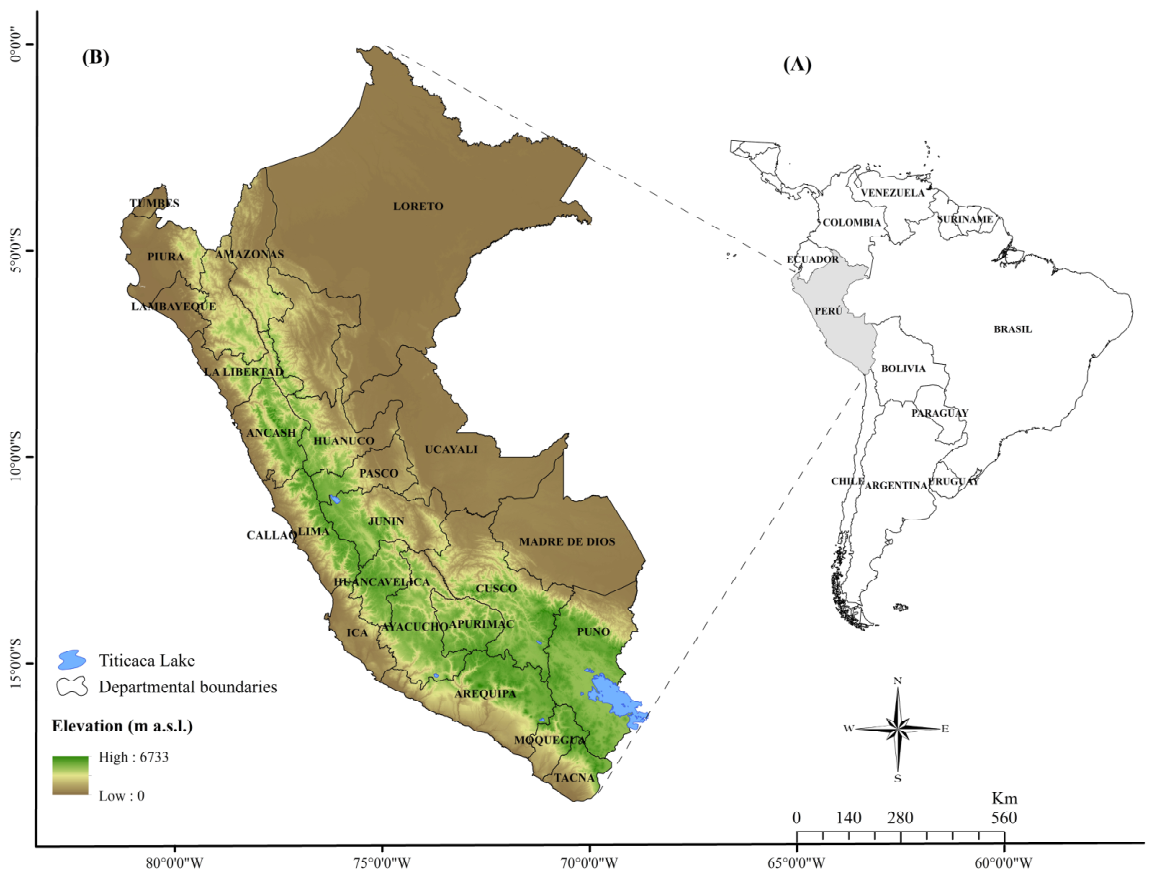
Figure 1. Location of the study area. (A) Location of Peru in South America. (B) Peru with departmental boundaries.
Forests 17 01126 g001
Figure 2. Variable selection. (A) Pearson correlation. (B) VIF values for variables.
Forests 17 01126 g002
Figure 3. Methodological Flowchart of the Process for Modeling the Habitat Suitability of the Genus Clusia L. in Peru Using MaxEnt.
Forests 17 01126 g003
Figure 4. Statistical metrics. (A) AUC-ROC, (B) Contribution variables, (C) Cumulative contribution.
Forests 17 01126 g004
Figure 5. Response Curves for the Variables Included in the Habitat Suitability Modeling of the Genus Clusia L. in Peru.
Forests 17 01126 g005
Figure 6. Current distribution and projected changes in habitat suitability for Clusia L. in Peru under climate change scenarios. (A) Current suitability. (B) Future suitability (2041–2100 period). (C) Spatiotemporal dynamics of change in habitat suitability.
Forests 17 01126 g006
Figure 7. Dynamics of change in the area of high habitat suitability for Clusia L. in Peru (2041–2100). (A) Projected reduction in suitable area under the SSPs. (B) Matrix of losses, gains, and percentages of change.
Forests 17 01126 g007
Figure 8. Spatial uncertainty (SD) among the three GCMs in projected suitability for Clusia L., by scenario and period.
Forests 17 01126 g008
Figure 9. Spatial difference in projected suitability between HadGEM3-GC31-LL and MPI-ESM1-2-HR, by scenario and period.
Forests 17 01126 g009
Table 1. Bioclimatic variables initially evaluated for modeling the potential distribution of the genus Clusia L. in Peru.
TypeCodeBioclimatic VariableUnitEcological Component Represented
BioclimaticBIO1 (*)Average annual temperature°CAnnual Heat Balance
BIO2 (*)Average daytime range°CDaily Temperature Variability
BIO3Isothermality%Relationship Between Daily and Annual Variation
BIO4 (*)Seasonal Variations in TemperatureDE × 100Seasonal Temperature Variability
BIO5 (*)Highest temperature in the warmest month°CMaximum thermal stress
BIO6 (*)Lowest temperature in the coldest month°CMinimum thermal limit
BIO7 (*)Annual temperature range°CAnnual temperature range
BIO8 (*)Average temperature of the wettest quarter°CTemperature Conditions During the Wet Season
BIO9 (*)Average temperature during the driest quarter°CTemperature Conditions During the Dry Season
BIO10 (*)Average temperature of the warmest quarter°CWarm thermal condition
BIO11 (*)Average temperature of the coldest quarter°CCold thermal condition
BIO12 (*)Annual precipitationmmAnnual Water Availability
BIO13 (*)Precipitation for the wettest monthmmMaximum monthly availability
BIO14 (*)Precipitation during the driest monthmmMonthly water deficit
BIO15Seasonal Variations in Precipitation%Seasonal Water Variability
BIO16Precipitation during the wettest quartermmMaximum water availability
BIO17 (*)Precipitation during the driest quartermmSeverity of the dry season
BIO18 (*)Precipitation during the warmest quartermmInteraction Between Heat and Humidity
BIO19Precipitation during the coldest quartermmWater Availability During the Cold Season
TopographicElevElevationm.a.s.lElevation in meters above sea level
Note: (*) variables with |r| ≥ 0.80.
Table 2. Current suitability area for Clusia L.
Suitability ClassArea (ha)Area (km2)% of Area Total
Unsuitable95,197,199.51951,972.0073.97%
Low12,121,560.69121,215.619.42%
Medium9,713,643.1697,136.437.55%
High11,664,519.77116,645.209.06%
Total128,696,923.131,286,969.23100.00%
Table 3. Future suitability area for Clusia L. under SSP2-4.5 and SSP5-8.5 scenarios.
SSPPeriodUnsuitableLowMediumHigh
ha%ha%ha%ha%
2-4.52041–2060103,249,960.1580.23%6,609,807.265.14%9,149,509.987.11%9,687,645.757.53%
2061–2080105,771,261.6482.19%6,060,334.034.71%8,494,816.766.60%8,370,510.716.50%
2081–2100105,760,624.5482.18%6,340,961.704.93%8,933,884.206.94%7,661,452.705.95%
5-8.52041–2060105,553,021.9882.02%6,659,090.095.17%9,106,559.557.08%7,378,251.525.73%
2061–2080107,057,506.2783.19%7,435,883.105.78%8,920,435.216.93%5,283,098.564.11%
2081–2100107,746,332.4483.72%6,888,574.095.35%9,162,605.787.12%4,899,410.833.81%
Table 4. Change in suitability area (future vs. current) for Clusia L.
SSPPeriodHigh LossLossNo ChangeGainHigh Gain
ha%ha%ha%ha%ha%
SSP2-4.52041–2060685,989.941.99%20,602,908.0259.62%9,085,772.9226.29%4,122,049.6611.93%61,409.360.18%
2061–20805,296,308.0815.23%18,942,465.7154.47%5,824,013.3116.75%4,419,831.8012.71%296,480.540.85%
2081–21007,060,022.3720.01%19,425,637.6555.07%3,944,866.8911.18%3,903,113.9011.06%942,959.462.67%
SSP5-8.52041–20606,638,869.8618.87%20,487,135.5858.24%4,006,323.4911.39%3,244,851.349.22%799,348.532.27%
2061–208013,432,921.3936.58%15,872,912.5843.22%1,691,677.164.61%2,718,716.067.40%3,009,916.478.20%
2081–210019,245,973.3350.43%10,224,721.3926.79%1,184,085.283.10%2,474,572.836.48%5,032,690.0013.19%
Disclaimer/Publisher’s Note: The statements, opinions and data contained in all publications are solely those of the individual author(s) and contributor(s) and not of MDPI and/or the editor(s). MDPI and/or the editor(s) disclaim responsibility for any injury to people or property resulting from any ideas, methods, instructions or products referred to in the content.