Spatial Patterns of Soil Water-Holding Capacity and Their Environmental Drivers in Spruce-Fir-Korean Pine Forest of the Xiaoxing’an Mountains

Abstract

In the primary spruce-fir-Korean pine forest affected by historical windthrow, soil water-holding capacity shows complex spatial associations with forest microenvironment and soil physicochemical properties. However, its spatial variability and multi-factor hierarchical association pathways remain poorly understood. Taking the primary spruce-fir-Korean pine forest on a historically windthrow-affected site in the Liangshui National Nature Reserve, Xiaoxing’an Mountains, China as the research object, geostatistics and partial least-squares structural equation modeling were used to analyze the spatial pattern of topsoil (0–20 cm) water-holding capacity and its environmental association pathways. The results showed saturated, capillary and field water-holding capacities of topsoil exhibited moderate variability and strong spatial autocorrelation (all nugget to sill ratios < 25%), showing a patchy distribution. No significant direct association was detected between windthrow mechanical disturbance intensity and topsoil water-holding capacity. Bulk density (path coefficient = −0.685, p < 0.001) and soil porosity (path coefficient = 0.273, p < 0.001) had significant direct associations with soil water-holding capacity, whereas soil particle size distribution showed no significant effect (p > 0.05). Canopy structure and understory microclimate exerted indirect associations with soil water-holding capacity via soil structure; litter showed no significant associative effect (p > 0.05). These results indicate that soil water-holding capacity on the historically windthrow-affected site was not randomly distributed, but presented an ordered patchy pattern closely related to in-plot micro-environmental factors.

1. Introduction

Forest soil water-holding capacity is a core indicator for evaluating ecosystem hydrological regulation and water conservation functions [1], and exerts important influences on surface runoff, water storage and catchment hydrological security [2]. Saturated water-holding capacity, capillary water-holding capacity and field water-holding capacity are key parameters for characterizing this capacity and are widely applied in the assessment of forest hydrological functions [3,4].

Numerous studies have explored the factors influencing forest soil water-holding capacity. Wang et al. [5] suggested that soil physical properties (bulk density, soil porosity) act as direct determinants of soil water-holding capacity; generally, lower bulk density and better-developed soil porosity correspond to higher soil water-holding capacity. Beyond intrinsic soil properties, canopy structure can indirectly modulate soil moisture conditions by altering under-canopy rainfall redistribution [6] and modifying understory microclimate [7]. Microclimatic conditions such as understory temperature and humidity can regulate soil water evaporation and infiltration processes [8]. The litter layer can participate in soil hydrological regulation via rainfall interception and reduction in surface evaporation [9]. Nevertheless, most existing studies focus on the relationships between individual environmental factors and soil water-holding capacity. Systematic analyses of multi-factor hierarchical regulatory pathways remain relatively scarce.

Windthrow represents a common natural disturbance [10]. It can generate forest gaps and pit-mound microtopography via canopy damage and tree uprooting [11], substantially alter stand structure [12] and surface microtopography [13] and further reshape understory microclimate as well as soil hydrothermal conditions [14]. Existing studies on soil hydrological properties have mostly focused on undisturbed steady-state stands, logged sites [15] and burned areas [16], with plantation and secondary forests as major research subjects [17]. Research on windthrow-affected natural forests, especially the zonal climax primary spruce-fir-Korean pine forest, remains rather limited. The Xiaoxing’an Mountains constitute a vital ecological barrier and water conservation region in China [18], where primary spruce-fir-Korean pine forests frequently suffer windthrow disturbances [19]. Nevertheless, the spatial patterns of soil water-holding capacity and its multi-factor regulatory pathways on historically windthrow-affected sites remain unclear. In particular, systematic quantitative analyses of hierarchical effects along the “canopy structure–understory microclimate–litter–soil structure” chain are scarce.

To date, no consistent conclusions have been reached regarding how soil water-holding capacity responds to forest disturbances. In studies covering different disturbance types and stand conditions, both increases and decreases in soil water-holding capacity have been reported [20]. Such inconsistent findings indicate that disturbance effects on soil hydrological functions are not unidirectionally driven by a single factor, but are predominantly governed by multi-factor interactions. The litter layer is recognized as an important regulatory node [21]. Nevertheless, its regulatory effect is not universal and exhibits strong environmental dependence across different ecosystems [22]. Accordingly, this study puts forward the following hypotheses: on windthrow-affected sites, canopy structure affects soil hydrological functions through an indirect cascading pathway of “canopy structure–understory microclimate–soil physical properties–soil water-holding capacity”; there is no significant direct association between windthrow mechanical disturbance intensity and topsoil water-holding capacity; and the direct regulatory effect of the litter layer is insignificant. Nevertheless, systematic quantitative verification of these hypothesized multi-factor hierarchical pathways remains lacking.

Therefore, this study investigated a primary spruce-fir-Korean pine forest with historical windthrow impacts in the Liangshui National Nature Reserve, Xiaoxing’an Mountains, China. Geostatistics were applied to characterize the spatial patterns of topsoil water-holding capacity. Combined with partial least-squares structural equation modeling (PLS-SEM), we revealed multi-factor hierarchical influence pathways on soil water-holding capacity from the perspective of the “canopy structure–understory microclimate–litter–soil structure” framework. The specific objectives of this study were as follows: (1) to clarify the spatial variability and distribution patterns of topsoil water-holding capacity under historical windthrow disturbance, and to examine spatial associations between windthrow disturbance intensity and topsoil water-holding capacity within the study site; (2) to disentangle direct and indirect environmental factors affecting soil water-holding capacity and quantify the pathways and effect magnitudes of each factor; and (3) to establish a hierarchical regulatory model of “canopy structure–understory microclimate–litter–soil structure–soil water-holding capacity” and identify key pathways sustaining soil hydrological functions on windthrow-affected sites. This work aims to provide a theoretical reference for ecological conservation and natural restoration management of regional primary spruce-fir-Korean pine forests on windthrow-disturbed sites.

2. Materials and Methods

2.1. Study Area

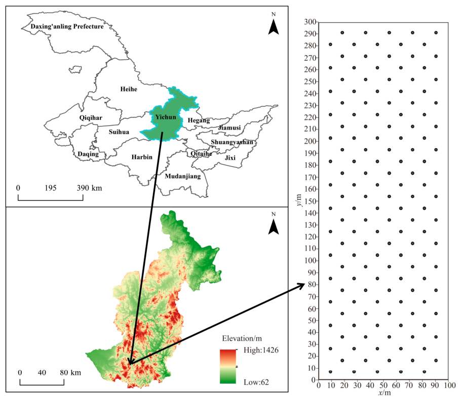
The study area is located in Liangshui National Nature Reserve, Heilongjiang Province, China (128°47′08″–128°57′19″ E, 47°06′49″–47°16′10″ N), on the southeastern branch of the Xiaoxing’an Mountains. It features low-hill and hilly landforms with an average elevation of approximately 400 m and has a temperate continental monsoon climate, characterized by long, cold and dry winters, as well as short summers with concurrent rainfall and high temperatures. The mean annual temperature is −0.3 °C, and the mean annual precipitation is 676 mm, with rainfall mainly concentrated from June to August. The zonal soil type is dark-brown forest soil. Temperate mixed coniferous broad-leaved forests dominated by Korean pine (Pinus koraiensis) prevail in the reserve. The main tree species include Pinus koraiensis, Picea koraiensis, Acer ukurunduense, Acer tegmentosum, Betula costata, Abies nephrolepis, Tilia amurensis, Acer mono and Syringa reticulata.

2.2. Plot Establishment and Vegetation Survey

In July 2024, a permanent 100 m × 300 m plot was established in a windthrow-affected spruce-fir-Korean pine forest within the study area. The plot was subdivided into 300 sub-plots of 10 m × 10 m using a grid-based sampling design. Obvious windthrow features were observed inside the plot, including stem breakage, root plates, leaning/fallen trees, tree uprooting and pit-mound microtopography. A total of 298 damaged living trees and 50 unidentifiable root plates were recorded, yielding 348 windthrow-related features in total. The criteria for identifying windthrow features included broken stems with fresh or old fracture surfaces, uprooted trees accompanied by pit-mound microtopography, leaning and fallen trees and residual root plates from windthrow events. Snags originating from natural senescence were not counted as windthrow features. Standing dead trees were classified as windthrow-caused mortality and included in statistics only if pit-mound microtopography caused by windthrow was present at their root bases [19,23]. Due to the lack of long-term monitoring records, the exact timing of single or multiple historical windthrow events generating these features cannot be determined in this study. Therefore, all references to “post-disturbance” in the manuscript denote the observed present-day status of the site, rather than results derived from time-series post-disturbance dynamic monitoring.

2.3. Sample Collection and Laboratory Measurements

2.3.1. Soil Sample Collection and Measurement

In June 2025, 150 sampling points were selected from the 300 grid sub-plots (10 m × 10 m) using a systematic S-shaped sampling scheme, whereby every alternate sub-plot was visited along an S-shaped route across the plot (see Figure 1 for the spatial distribution of sampling points). At each sampling point, three undisturbed core samples (0–20 cm depth) were collected around the centre of the selected sub-plot. Their average values represented soil physical properties for that sampling point to reduce sampling errors caused by micro-scale spatial variability in forest topsoil. Bulk density, soil porosity and soil water-holding capacity were measured using the core sampling method [5]. Let m₀ = mass of the metal core ring, m₁ = total mass of core ring plus undisturbed soil and m₂ = mass of the aluminium box; the undisturbed soil core was submerged in water for 12 h and weighed (recorded as m₃). The saturated core ring was placed on a tray filled with dry sand for 2 h and weighed (recorded as m₄). After a further 48 h, the core was weighed again (recorded as m₅). Approximately 20 g of representative soil was taken from the core ring, placed in a pre-weighed aluminium box and weighed (recorded as m₆). The subsample was then oven-dried at 105 °C for 8 h to constant mass and re-weighed (recorded as m₇). Total porosity, capillary porosity, non-capillary porosity and bulk density were calculated from the above mass measurements. Saturated water-holding capacity, capillary water-holding capacity and field water-holding capacity were further derived. The calculation formulas are shown below:

$$\begin{gathered} K_1=\left(m_7-m_2\right)/\left(m_6-m_2\right) \\ {m}_{dry}=\left(m_1-m_0\right)\times K_1 \\ BD=m_{dry}/V \\ \mathrm{S}\mathrm{a}\mathrm{t}\mathrm{u}\mathrm{r}\mathrm{a}\mathrm{t}\mathrm{e}\mathrm{d} \mathrm{W}\mathrm{H}\mathrm{C}=\left[\left(m_3-m_0\right)-m_{dry}\right]/m_{dry}\times 100 \\ \mathrm{F}\mathrm{i}\mathrm{e}\mathrm{l}\mathrm{d} \mathrm{W}\mathrm{H}\mathrm{C}=\left[\left(m_4-m_0\right)-m_{dry}\right]/m_{dry}\times 100 \\ \mathrm{C}\mathrm{a}\mathrm{p}\mathrm{i}\mathrm{l}\mathrm{l}\mathrm{a}\mathrm{r}\mathrm{y} \mathrm{W}\mathrm{H}\mathrm{C}=\left[\left(m_5-m_0\right)-m_{dry}\right]/m_{dry}\times 100 \\ \mathrm{N}\mathrm{C}\mathrm{P}=\left(\mathrm{S}\mathrm{W}\mathrm{H}\mathrm{C}-\mathrm{C}\mathrm{W}\mathrm{H}\mathrm{C}\right)\times \mathrm{B}\mathrm{D} \\ \mathrm{C}\mathrm{P}=\mathrm{C}\mathrm{W}\mathrm{H}\mathrm{C}\times \mathrm{B}\mathrm{D} \\ \mathrm{T}\mathrm{P}=\mathrm{N}\mathrm{C}\mathrm{P}+\mathrm{C}\mathrm{P} \end{gathered}$$

where $K_1$ is the moisture conversion coefficient; $m_{dry}$ is the mass of oven-dried soil inside the metal core ring (g); V is the volume of the core ring, 100 cm³; TP is total porosity (%); CP is capillary porosity (%); and NCP is non-capillary porosity (%).

Saturated, capillary and field water-holding capacities obtained via the core sampling method in this study represent intrinsic soil hydrological properties measured under laboratory conditions, which differ from temporally variable in situ soil water content influenced by meteorological conditions in the field.

Approximately 500 g of composite soil samples were simultaneously collected for soil particle size distribution analysis. The pipette method was adopted for measurements [24], with NaOH solution used as the dispersing agent.

2.3.2. Canopy Structure Measurement

Hemispherical photography was used to acquire canopy images above each soil sampling point. A Canon EOS 50D digital camera (Canon Inc., Tokyo, Japan) fitted with a Sigma EX DG 8 mm fisheye lens (Sigma Corporation, Kawasaki, Japan) was mounted on a tripod at 1.5 m above the ground, with the lens oriented vertically upward for canopy photography. Photography was conducted under uniform light conditions during early morning or overcast days. Three consecutive hemispherical (full-sky) photographs were taken at the centre of each sub-plot. HemiView 2.1 canopy analysis software was used for image interpretation. Plot latitude, longitude and elevation data were imported. Automatic threshold segmentation combined with manual fine tuning was applied to process images. Output parameters included leaf area index (LAI), mean leaf angle (MLA), ground cover (GndCover), visible sky fraction (VisSky), effective leaf area density (ELADP) and coefficient of variation of leaf area index (LAIDev).

2.3.3. Litter Collection and Measurement

Three 0.5 m × 0.5 m sub-plots were arranged along the diagonal within each soil sampling plot. All litter within each sub-plot was collected and placed into paper bags. Fresh mass was measured in the field. Samples were transported to the laboratory and oven-dried at 65 °C to constant mass (the mass difference between two successive weighings < 0.01 g). Dry mass was recorded. Surface litter mass (LM, g/m²) and litter moisture content (LMC, %) were calculated according to the following formulas:

$$\begin{gathered} \mathrm{L}\mathrm{M}={\displaystyle \raisebox{1ex}{$W_{dry}$}\!\left/ \!\raisebox{-1ex}{$0.25$}\right.} \\ \mathrm{L}\mathrm{M}\mathrm{C}={\displaystyle \raisebox{1ex}{$W_{fresh}-W_{dry}$}\!\left/ \!\raisebox{-1ex}{$W_{dry}$}\right.}\times 100\% \end{gathered}$$

where $W_{dry}$ is the dry litter mass of a single sub-plot (g), $W_{fresh}$ is the fresh litter mass of a single sub-plot (g) and 0.25 is the sub-plot area (m²). Finally, the average value from the three sub-plots was taken to represent litter characteristics for each sampling point.

2.3.4. Understory Microclimate Factor Measurement

Under the growing season from June to October 2025, six representative sunny days were selected each month for understory microclimate measurements. A quantum/illuminance dual-radiometer (Apogee Instruments Inc., Logan, UT, USA) was used to measure photosynthetic photon-flux density (PPFD, μmol·m⁻²·s⁻¹) at 1.5 m above each soil sampling point. An infrared thermometer was applied to obtain surface-soil temperature (SST, °C). A digital thermocouple probe thermometer (Spectrum Technologies, Inc., Aurora, IL, USA) was used to measure soil temperature at 20 cm depth (ST, °C). A digital temperature–humidity meter (TES Electrical Electronic Corp., Taiwan, China) measured air temperature (AT, °C) and relative humidity (RH, %) at 1.5 m above the ground surface. Mean values calculated from all observations collected from June to October at each sampling point were used for subsequent statistical analyses.

2.4. Data Processing and Statistical Analyses

2.4.1. Semivariogram

The semivariogram was applied to characterize the spatial heterogeneity of soil water-holding capacity and forest micro-environmental factors. Its calculation formula is given below:

$$\mathsf{\gamma }\left(h\right)={\displaystyle \frac{1}{2N\left(h\right)}}{\sum }_{i=1}^{N_{\left(h\right)}}{\left[Z\left(x_i\right)-Z\left(x_i+h\right)\right]}^2$$

where $\mathsf{\gamma }\left(h\right)$ is the semivariogram value; $N\left(h\right)$ is the number of point pairs separated by distance h; and $Z\left(x_i\right)$ and $Z\left(x_i+h\right)$ are the observed values at sample locations $x_i$ and $x_i+h$, respectively [25].

In the semivariogram, the range (A₀) reflects the spatial autocorrelation distance. Samples exhibit spatial autocorrelation within the range; beyond this range, no spatial autocorrelation exists among samples [26]. The nugget to sill ratio (the ratio of nugget variance to sill variance) quantifies the strength of spatial autocorrelation: values < 25% indicate strong spatial autocorrelation; values between 25% and 75% indicate moderate spatial autocorrelation; and values > 75% indicate weak spatial autocorrelation, implying that spatial variability is dominated by random factors, and such variables are unsuitable for spatial interpolation [27]. The coefficient of variation (CV) measures the degree of data dispersion for each indicator: CV < 10% represents weak variability; 10% ≤ CV ≤ 100% represents moderate variability; and CV > 100% represents strong variability.

During semivariogram fitting, the lag interval was set to 12 m according to the average distance between sampling points. Isotropic models were used for semivariogram fitting [28]. The optimal model among Gaussian, exponential and spherical models was selected by minimizing the residual sum of squares (RSS) and maximizing the coefficient of determination (R²). To assess the prediction accuracy of Kriging interpolation, leave-one-out cross-validation was performed for the optimal fitted model. Evaluation metrics including mean error (ME), root-mean-square error (RMSE) and average standard error (ASE) were calculated.

2.4.2. Global Moran’s I

The Global Moran’s I index was applied to test the significance of spatial autocorrelation for each soil water-holding capacity indicator. Global Moran’s I ranges from −1 to 1. Positive values indicate positive spatial autocorrelation, whereas a value of zero indicates a spatially random distribution of variables [29]. The Z-score approach was used for significance testing, with the significance level set at p < 0.05.

2.4.3. Spatial Association Analysis Between Windthrow Features and Soil Sampling Points

To examine the spatial association between windthrow disturbance intensity and soil water-holding capacity, spatial coordinates of 348 windthrow features were used to generate a continuous surface of plot-scale windthrow disturbance intensity via Kernel Density Estimation in ArcGIS 10.7. Disturbance intensity values were then extracted to the 150 soil sampling points. Windthrow features were further classified into a high-mechanical-disturbance group (root plates, fallen trees and stem breakage) and a low/no-mechanical-disturbance group (snags, leaning/bent trees) according to disturbance mechanisms [30]. A spatial buffer with a 10 m radius was created centred on each soil sampling point, and the spatial join tool was applied to assign the corresponding disturbance type to each sampling point.

Spearman correlation analysis was performed to examine the relationships between windthrow kernel density values and each soil water-holding capacity indicator. Independent-samples T-test was used to compare group differences in soil water-holding capacity between high- and low-disturbance groups. Cohen’s d effect size was calculated to evaluate the practical magnitude of between-group differences: Cohen’s d < 0.2 indicates a small effect; 0.2–0.5 indicates a moderate effect; and >0.5 indicates a large effect.

2.4.4. Partial Least-Squares Structural Equation Modelling (PLS-SEM)

Partial least-squares structural equation modelling (PLS-SEM) was used to disentangle direct and indirect influence paths of environmental factors on soil water-holding capacity. Model construction and analysis were implemented using SmartPLS 4.1 software. Prior to model estimation, variance inflation factor (VIF) was applied for collinearity diagnosis. No severe multicollinearity was assumed when inner VIF values of all predictor variables in the structural model were below the critical threshold of 5.0 [31]. Cronbach’s α and composite reliability were used to assess the internal consistency of the model, and average variance extracted was calculated to examine convergent validity. The bootstrap resampling procedure was adopted to test the significance of path coefficients with 5000 resamples. The 95% bias-corrected bootstrap confidence intervals (bias-corrected bootstrap CI) for indirect effects were also computed.

To detect potential unexplained spatial autocorrelation in PLS-SEM model residuals, inner-model residuals of the latent variable for soil water-holding capacity were extracted, and the Global Moran’s I index was used to perform spatial autocorrelation tests on these residuals. The Global Moran’s I was computed using the inverse-distance conceptualization of spatial relationships, with Euclidean distance used to measure distances between sampling points, and row-standardized spatial weights were implemented. Although sampling points were laid out with relatively even spacing, inverse-distance weighting captured the continuous decay of soil attribute similarity across geographic distance and avoided artificial cut-off effects caused by k-nearest-neighbour specifications. Significance assessment was performed using 999 Monte Carlo permutations. For this inverse-distance weighting, the bandwidth was set to 0 with no distance cut-off threshold, meaning all sampling point pairs were included in weight matrix construction.

2.4.5. Data Processing

Microsoft Excel 2021 was used for preliminary data processing. Descriptive statistics for all variables were computed in SPSS 27.0. The K–S (Kolmogorov–Smirnov) test was applied for normality testing (p > 0.05 indicates that data follow a normal distribution). Data that failed the normality test were log-transformed (base-10 logarithm). The transformed datasets were used for subsequent geostatistical analyses and ordinary Kriging interpolation. GS+ 9.0 was employed for semivariogram analysis and model parameter optimization. Ordinary Kriging interpolation for soil water-holding capacity indicators was implemented in ArcGIS 10.7 to generate spatial distribution maps. Spearman correlation analysis was conducted for pairwise relationships between forest micro-environmental factors and soil water-holding capacity indicators. Two-tailed tests were performed at significance levels of 0.01 and 0.05, and correlation matrix plots were produced using Origin 2026. SmartPLS 4.1 was used to construct the partial least-squares structural equation model, and the goodness-of-fit statistic was applied to evaluate the overall model performance.

3. Results

3.1. Spatial Variation Characteristics of Forest Micro-Environmental Factors

3.1.1. Descriptive Statistics of Forest Micro-Environmental Factors

Descriptive statistics for canopy structure and understory microclimate factors are summarized in

Table 1. Descriptive statistics of canopy structure and understory micro-environment factors (n = 150).

Category	Indicators	Min	Max	Mean	SD	CV/%	Skewness	Kurtosis	K–S Statistic
Canopy structure	LAI	1.386	13.214	3.303	1.466	44.38	2.934	14.645	0.163
	GndCover	0.003	0.997	0.864	0.157	18.11	−2.917	11.468	0.206
	MLA	0.038	89.986	24.112	21.803	90.43	1.414	1.444	0.160
	VisSky	0.003	0.234	0.065	0.046	71.38	1.148	1.094	0.139
	ELADP	0.001	501.068	11.992	41.555	346.52	11.111	131.029	0.386
	LAIDev	1.776	10.443	4.322	1.257	29.09	2.192	8.188	0.162
Understory microclimate factors	PPFD	37.533	801.833	239.547	150.212	62.71	1.122	1.044	0.116
	RH	46.913	62.500	53.400	2.985	5.59	0.625	0.014	0.092
	AT	20.057	26.227	23.126	0.899	3.89	−1.032	2.508	0.142
	ST	10.683	14.953	12.992	0.645	4.97	−0.065	0.612	0.044
	SST	18.103	24.773	20.792	1.201	5.78	0.576	0.935	0.067

Note: LAI, leaf area index; GndCover, ground cover; MLA, mean leaf angle; VisSky, visible sky fraction; ELADP, effective leaf area density; LAIDev, coefficient of variation of leaf area index; PPFD, photosynthetic photon-flux density; RH, relative humidity; AT, air temperature; ST, soil temperature (0–20 cm depth); SST, surface-soil temperature (0 cm); K–S, Kolmogorov–Smirnov; SD, standard deviation; and CV, coefficient of variation.

. Among canopy structure variables, the CV of ELADP reached 346.52%, indicating strong spatial variability. The CV of the remaining canopy structure indicators ranged from 10% to 100%, corresponding to moderate spatial variability. For understory microclimate factors, the CV of PPFD was 62.71%, representing moderate spatial variability. The CV of relative humidity, air temperature, soil temperature and surface-soil temperature were all lower than 10%, showing weak spatial variability.

Descriptive statistics for litter and topographic factors are summarized in

Table 2. Descriptive statistics of litter and topographic factors (n = 150).

Category	Indicators	Min	Max	Mean	SD	CV/%	Skewness	Kurtosis	K–S Statistic
Litter	LM	30.920	758.960	264.094	135.001	51.12	0.945	1.010	0.108
	LMC	0.190	1.305	0.622	0.208	33.45	0.567	−0.101	0.091
Topographic factors	Elevation	381.390	406.330	391.252	3.659	0.94	0.347	1.746	0.054
	Slope	0.000	21.000	8.207	5.045	61.48	0.462	−0.411	0.117

Note: LM, litter mass; LMC, litter moisture content.

. The CV of surfaceLM and LMC was 51.12% and 33.45%, respectively, both indicating moderate spatial variability. For topographic factors, the CV of elevation was 0.94%, representing weak spatial variability, whereas the CV of slope was 61.48%, indicating moderate spatial variability.

Descriptive statistics for soil physical structure and soil particle size distribution are summarized in

Table 3. Descriptive statistics of soil physical structure and soil particle size distribution (n = 150).

Category	Indicators	Min	Max	Mean	SD	CV/%	Skewness	Kurtosis	K–S Statistic
Soil physical structure	BD	0.260	1.275	0.607	0.206	33.84	0.907	0.877	0.108
	TP	46.055	94.488	80.730	8.263	12.09	−1.465	2.715	0.135
	CP	45.545	89.013	75.012	7.887	13.12	−0.971	1.301	0.099
	NCP	0.373	29.740	5.719	5.524	94.89	1.593	2.702	0.168
Soil particle size distribution	Clay	3.635	39.582	22.547	6.178	27.40	−0.059	−0.136	0.066
	Silt	17.281	52.099	33.577	4.944	14.72	0.316	1.380	0.070
	Sand	25.442	60.011	43.876	7.544	17.19	−0.254	−0.479	0.050

Note: BD, bulk density; TP, total porosity; CP, capillary porosity; and NCP, non-capillary porosity. The humus topsoil of this forest had relatively high organic matter content. Total porosity exceeded 80% in some soil samples, which is an observable feature of humus-rich forest soils [32].

. The CV for bulk density, soil porosity and all soil particle size distribution indicators ranged from 10% to 100%, indicating moderate spatial variability.

3.1.2. Semivariogram Analysis

Semivariogram analysis was performed for canopy structure and understory microclimate factors (

Table 4. Semivariogram parameters for canopy structure and understory micro-environment factors (n = 150).

Category	Indicators	Model Type	C0	Sill (C0 + C)	C0/(C0 + C)/%	C/(C0 + C)/%	A0/m	R2	Residual SS
Canopy structure	LAI	Gaussian	0.06500	0.13500	48.1	51.9	71.54	0.964	1.340 × 10−4
	GndCover	Exponential	0.00329	0.02598	12.7	87.3	30.90	0.681	8.184 × 10−6
	MLA	Exponential	0.02500	0.64300	3.9	96.1	38.40	0.681	0.0101
	VisSky	Spherical	1.980 × 10−4	2.046 × 10−3	9.7	90.3	100.90	0.988	2.893 × 10−8
	ELADP	Exponential	0.04700	0.95100	4.9	95.1	32.40	0.499	0.0320
	LAIDev	Spherical	0.04040	0.08120	49.8	50.2	134.90	0.965	4.571 × 10−5
Understory microclimate factors	PPFD	Gaussian	0.21550	0.47900	45.0	55.0	160.56	0.992	3.870 × 10−4
	RH	Gaussian	6.700 × 10−4	5.830 × 10−3	11.5	88.5	199.19	0.986	2.635 × 10−7
	AT	Gaussian	3.340 × 10−4	2.648 × 10−3	12.6	87.4	227.42	0.996	1.257 × 10−8
	ST	Exponential	2.520 × 10−4	2.564 × 10−3	9.8	90.2	45.30	0.902	8.910 × 10−8
	SST	Gaussian	1.300 × 10−3	4.510 × 10−3	28.8	71.2	132.50	0.968	3.539 × 10−7

Note: C₀: nugget variance; sill (C₀ + C): sill variance; C₀/(C₀ + C): nugget to sill ratio; C/(C₀ + C): structural variance ratio; A₀: range; R²: coefficient of determination; and residual SS: residual sum of squares. Semivariogram models with R² < 0.6 exhibit poor fitting performance, and their spatial structure parameters are only for descriptive reference.

). For canopy structure variables, the optimal semivariogram model for LAI was the Gaussian model; the optimal models for GndCover, MLA and ELADP were exponential models; VisSky and LAIDev were best fitted by the spherical model. The nugget to sill ratios of LAI (48.1%) and LAIDev (49.8%) ranged from 25% to 75%, indicating moderate spatial autocorrelation. The nugget-to-sill ratios of the remaining canopy structure indicators were below 25%, showing strong spatial autocorrelation. Among understory microclimate factors, only ST was best fitted by the exponential model, whereas all other variables adopted the Gaussian model as their optimal model. The nugget to sill ratios of PPFD (45.0%) and SST (28.8%) fell within 25–75%, representing moderate spatial autocorrelation.

Semivariogram analysis was carried out for litter and topographic factors (

Table 5. Semivariogram parameters for litter and topographic factors (n = 150).

Category	Indicators	Model Type	C0	Sill (C0 + C)	C0/(C0 + C)/%	C/(C0 + C)/%	A0/m	R2	Residual SS
Litter	LM	Exponential	0.03020	0.31340	9.6	90.4	32.70	0.653	1.361 × 10−3
	LMC	Gaussian	0.06650	0.16700	39.8	60.2	198.67	0.988	9.549 × 10−5
Topographic factors	Elevation	Spherical	3.950 × 10−5	1.010 × 10−4	39.1	60.9	145.00	0.982	5.110 × 10−11
	Slope	Exponential	0.02800	0.46900	6.0	94.0	21.90	0.145	7.608 × 10−3

Note: Semivariogram models with R² < 0.6 exhibit poor fitting performance, and their spatial structure parameters are only for descriptive reference.

). The optimal semivariogram models for LM and slope were the exponential model; LMC was best fitted by the Gaussian model, and elevation by the spherical model. The nugget to sill ratios of LMC (39.8%) and elevation (39.1%) ranged from 25% to 75%, indicating moderate spatial autocorrelation. The nugget to sill ratios of LM and slope were both below 25%, showing strong spatial autocorrelation.

Semivariogram analysis was performed for soil physical structure and soil particle size distribution (

Table 6. Semivariogram parameters for soil physical structure and soil particle size distribution (n = 150).

Category	Indicators	Model Type	C0	Sill (C0 + C)	C0/(C0 + C)/%	C/(C0 + C)/%	A0/m	R2	Residual SS
Soil physical structure variables	BD	Exponential	0.00216	0.01592	13.6	86.4	48.90	0.775	4.916 × 10−6
	TP	Exponential	0.00166	0.01342	12.4	87.6	39.60	0.301	1.661 × 10−5
	CP	Exponential	0.00127	0.01304	9.7	90.3	24.60	0.311	5.547 × 10−6
	NCP	Exponential	0.0970	1.0630	9.1	90.9	21.00	0.182	0.0223
Soil particle size distribution	Clay	Exponential	0.00890	0.10080	8.8	91.2	24.90	0.303	2.555 × 10−4
	Silt	Gaussian	0.00312	0.02304	13.5	86.5	12.99	0.002	7.591 × 10−6
	Sand	Linear	0.04579	0.04579	100.0	0	103.77	0.421	1.965 × 10−5

Note: Semivariogram models with R² < 0.6 exhibit poor fitting performance, and their spatial structure parameters are only for descriptive reference.

). The optimal semivariogram models for soil physical structure variables and clay were exponential models. Silt and sand were best fitted by the Gaussian model and linear model, respectively. Sand exhibited a pure-nugget effect with a nugget to sill ratio of 100%, indicating a nearly random spatial distribution. The nugget to sill ratios of the remaining factors were all below 25%, showing strong spatial autocorrelation.

3.2. Descriptive Statistical Characteristics and Spatial Distribution of Soil Water-Holding Capacity

3.2.1. Descriptive Statistics of Soil Water-Holding Capacity

In the study plot, the mean values of soil saturated water-holding capacity, capillary water-holding capacity and field water-holding capacity were 157.26%, 144.24% and 138.40%, respectively. Their CVs were 40.60%, 37.34% and 36.93%, all indicating moderate spatial variability (

Table 7. Descriptive statistics of soil water-holding capacity (n = 150).

Indicators	Min	Max	Mean	SD	CV/%	Skewness	Kurtosis	K–S Statistic	Distribution Type
Saturated WHC/%	41.22	328.64	157.26	63.85	40.60	0.633	−0.091	0.097	*
Capillary WHC/%	40.70	293.67	144.24	53.86	37.34	0.573	0.136	0.089	*
Field WHC/%	38.73	286.77	138.40	51.11	36.93	0.562	0.227	0.082	*

Note: WHC, water-holding capacity; * indicates that the raw data conform to a normal distribution after log-transformation.

).

3.2.2. Semivariogram Analysis and Global Moran’s I

Semivariogram modelling was performed for soil water-holding capacity (

Table 8. Semivariogram parameters and p-values (n = 150).

Indicators	Model Type	C0	Sill (C0 + C)	C0/(C0 + C)/%	C/(C0 + C)/%	A0/m	R2	Residual SS	Moran’s I	Z-Score	p-Value
Saturated WHC	Exponential model	0.02860	0.19720	14.5	85.5	53.4	0.751	9.927 × 10−4	0.05802	3.43556	0.00059
Capillary WHC	Exponential model	0.02330	0.16760	13.9	86.1	51.0	0.717	7.758 × 10−4	0.05158	3.09561	0.00194
Field WHC	Exponential model	0.02220	0.16440	13.5	86.5	48.9	0.687	7.822 × 10−4	0.05049	2.84444	0.00445

Note: All p-values for Moran’s I were <0.01, indicating significant spatial autocorrelation.

). The optimal fitted model for saturated water-holding capacity, capillary water-holding capacity and field water-holding capacity was the exponential model, with coefficients of determination of 0.751, 0.717 and 0.687, respectively. The residual sum of squares was generally low, indicating satisfactory model performance for characterizing the spatial variation structure of soil water-holding capacity in the spruce-fir-Korean pine mixed forest. The nugget to sill ratios of all indicators were below 25%, showing strong spatial autocorrelation. This suggests that spatial variability in soil water-holding capacity was dominated by structural factors, with limited contributions from random factors. The range varied from 48.9 m to 53.4 m, implying significant spatial autocorrelation for soil water-holding capacity indicators within this distance. Ordinary Kriging interpolation was implemented based on the optimal semivariogram models. Results of leave-one-out cross-validation are shown in

Table 9. Statistical results of leave-one-out cross-validation for Kriging interpolation of soil water-holding capacity.

Indicators	ME	RMSE	MSE	ASE	RMSSE
Saturated WHC	0.0007325	0.66123	−0.06398696	0.6100343	1.127616
Capillary WHC	−0.0004816	0.5619427	−0.06383714	0.5162327	1.135823
Field WHC	0.00008896175	0.5378576	−0.06403996	0.4955373	1.135817

Note: ME, mean error; RMSE, root-mean-square error; MSE, mean standardized error; ASE, average standard error; and RMSSE, root-mean-square standardized error.

. The root-mean-square standardized error values for all indicators were close to 1, indicating reliable Kriging interpolation predictions.

Global Moran’s I analysis yielded Moran’s I values of 0.058, 0.052 and 0.050 of saturated water-holding capacity, capillary water-holding capacity and field water-holding capacity, respectively (p < 0.01). These results indicate significant positive spatial autocorrelation for soil water-holding capacity within the study plot, characterised by high-high and low-low spatial clustering patterns rather than a random distribution.

3.2.3. Spatial Distribution Patterns of Soil Water-Holding Capacity

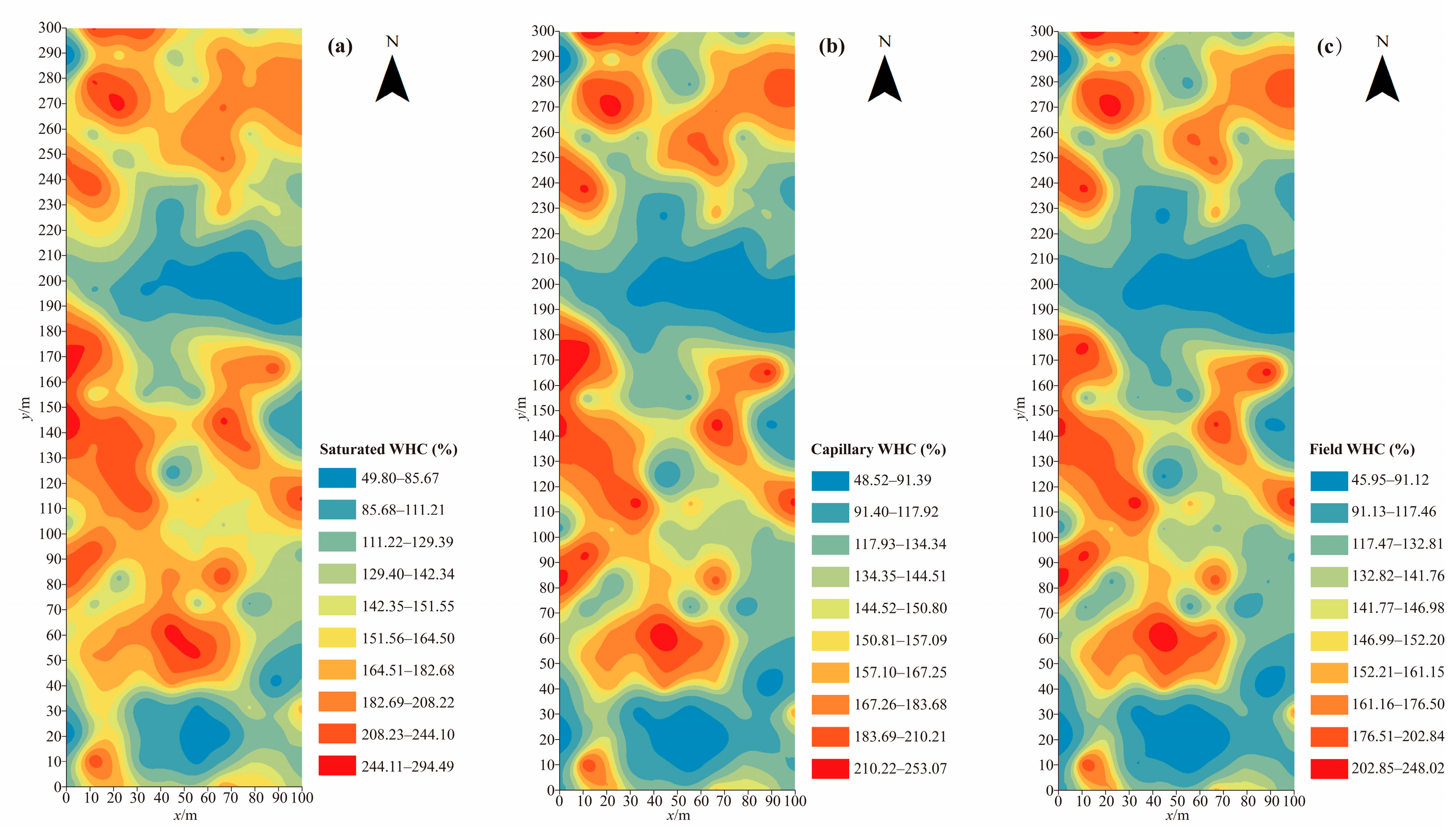
Kriging interpolation was performed based on the optimal semivariogram models (Figure 2). The spatial distribution patterns of saturated water-holding capacity, capillary water-holding capacity and field water-holding capacity were highly similar and exhibited distinct patchy clustering features. High-value zones were mainly located in the northern, southwestern and southern parts of the plot, whereas low-value zones were concentrated and continuously distributed in the central area. The high- and low-value extents largely overlapped across the three indicators, showing strong consistency in their spatial patterns.

Graded area statistics (

Table 10. Area proportions of graded soil water-holding capacity based on interpolation.

Zoning of Soil Water-Holding Capacity	Proportion of Graded Area/%	Saturated WHC	Capillary WHC	Field WHC
Low-value zone	20.75	21.79	20.91	20.46
Medium-value zone	47.94	47.79	48.22	47.36
High-value zone	31.31	30.42	30.86	32.18

Note: The grading of soil water-holding capacity was based on Kriging interpolation results and classified into low, medium, and high levels using the Natural Breaks method; proportions refer to the ratio of each graded zone area to the total plot area.

) revealed that the medium-value zones accounted for the largest proportion of area, all close to 50%, followed by high-value zones, while low-value zones occupied the smallest proportion. The differences in the proportional area of the three graded classes were all less than 2%, which further confirmed the high consistency of their spatial distributions.

3.3. Analysis of Influencing Factors for Soil Water-Holding Capacity

3.3.1. Spatial Association Between Windthrow Disturbance Intensity and Soil Water-Holding Capacity

Results of kernel density correlation analysis and group comparisons (

Table 11. Comparison of soil water-holding capacity under different mechanical disturbance types.

Indicators	Kernel Density Correlation Coefficient (r)	p-Value (Correlation)	High-Disturbance Group	Low-Disturbance Group	t-Value	p-Value (t-Test)	Cohen’s d
Saturated WHC	0.104	0.205	161.36 ± 60.36	150.58 ± 69.20	1.003	0.317	0.17
Capillary WHC	0.102	0.214	147.77 ± 50.63	138.48 ± 58.77	1.026	0.307	0.17
Field WHC	0.105	0.201	141.93 ± 48.64	132.65 ± 54.87	1.080	0.282	0.18

Note: Data are presented as “mean ± standard deviation”; p > 0.05 indicates non-significant differences between the two groups; and Cohen’s d < 0.2 represents a small effect size.

) showed that no significant statistical associations were detected between windthrow kernel density values, mechanical disturbance groups and topsoil water-holding capacity at the current observation stage (p > 0.05). Cohen’s d effect sizes for between-group differences ranged from 0.17 to 0.18, corresponding to a small effect magnitude.

3.3.2. Correlation Analysis Between Various Factors and Soil Water-Holding Capacity

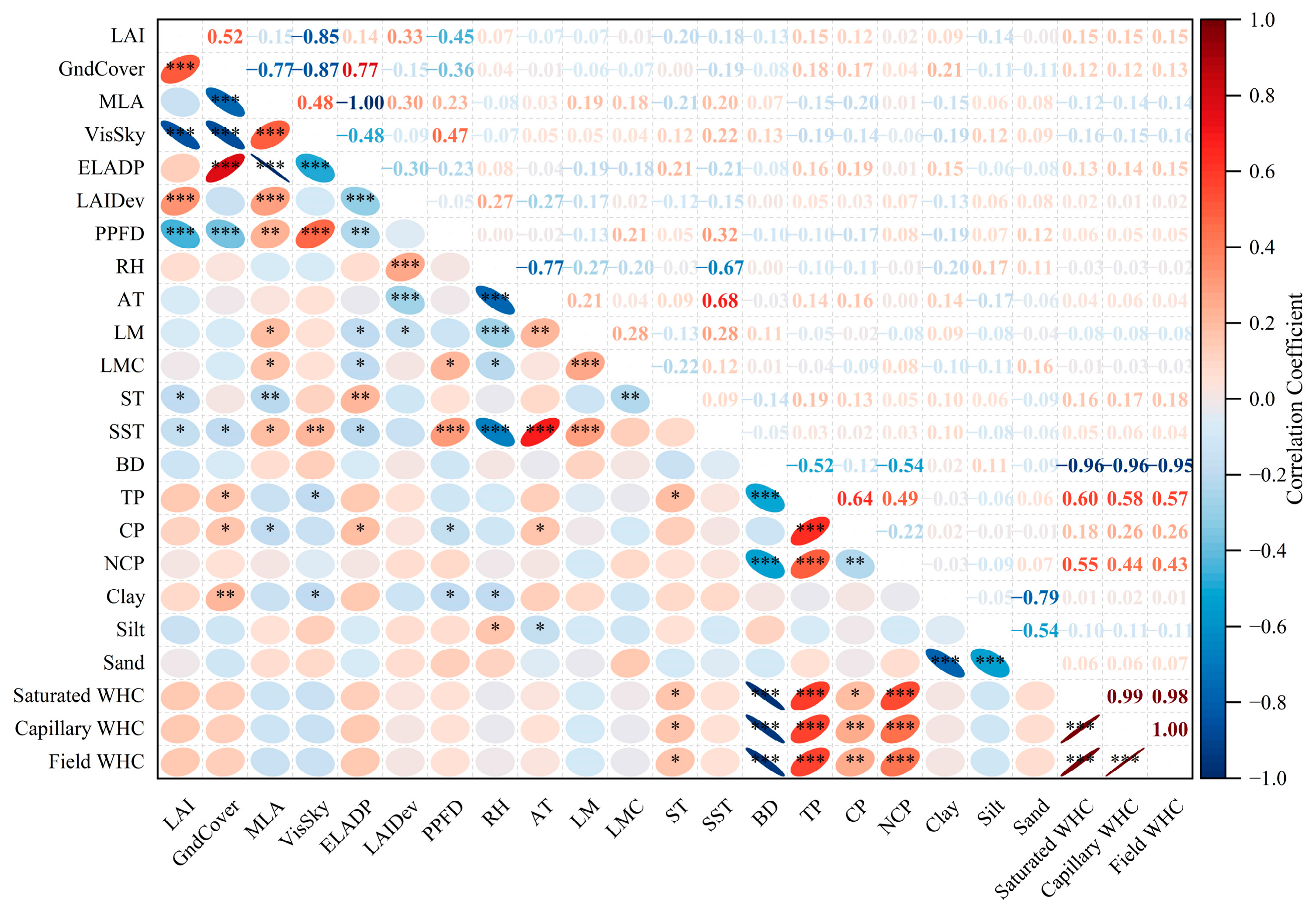
Spearman correlation analysis (Figure 3) revealed that saturated water-holding capacity, capillary water-holding capacity and field water-holding capacity were all highly significantly negatively correlated with bulk density (p < 0.001), and highly significantly positively correlated with total porosity, capillary porosity and non-capillary porosity (p < 0.001). They showed a significant positive correlation with soil temperature (p < 0.05), albeit with low correlation coefficients. No significant correlations (p > 0.05) were detected between soil water-holding capacity indicators and soil particle size distribution (clay, silt, sand), litter mass, litter moisture content, elevation and slope, as well as all canopy structure and understory microclimate factors.

3.3.3. Direct and Indirect Effects of Factors on Soil Water-Holding Capacity

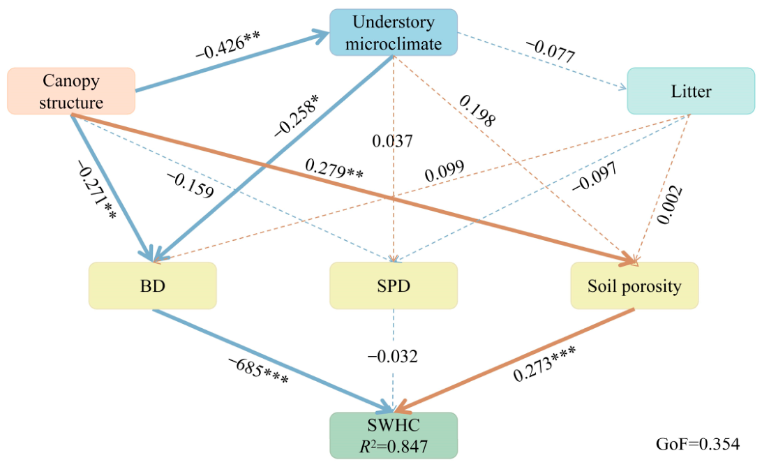
PLS-SEM revealed the direct and indirect pathways of various factors affecting soil water-holding capacity (Figure 4). Bulk density exerted a highly significant negative direct effect on soil water-holding capacity (path coefficient = −0.685, p < 0.001), whereas soil porosity had a highly significant positive direct effect (path coefficient = 0.273, p < 0.001).

Canopy structure influenced soil water-holding capacity mainly via three indirect pathways: “canopy structure → understory microclimate → bulk density → soil water-holding capacity”, “canopy structure →bulk density → soil water-holding capacity” and “canopy structure → soil porosity → soil water-holding capacity”. Canopy structure exerted a highly significant negative direct effect on understory microclimate (path coefficient = −0.426, p < 0.01), a highly significant negative direct effect on bulk density (path coefficient = −0.271, p < 0.01) and a highly significant positive direct effect on soil porosity (path coefficient = 0.279, p < 0.01). Understory microclimate had a significant negative direct effect on bulk density (path coefficient = −0.258, p < 0.05), thereby indirectly affecting soil water-holding capacity. No significant direct effects of understory microclimate on soil porosity and soil particle size distribution were detected (p > 0.05).

Neither direct nor indirect effects of litter on bulk density, soil porosity and soil water-holding capacity were significant (p > 0.05). In addition, the direct effect of soil particle size distribution on soil water-holding capacity was also non-significant (path coefficient = −0.032, p > 0.05).

Results of the model indirect-effect tests (

Table 12. Test of indirect effects in the PLS-SEM model.

Indirect Path	Path Coefficient	95% CI (Bias-Corrected)	p
Canopy structure → bulk density → SWHC	0.186	[0.057, 0.305]	0.004
Canopy structure → soil porosity → SWHC	0.076	[0.025, 0.153]	0.018
Understory micro-environment → bulk density → SWHC	0.177	[−0.032, 0.320]	0.039
Canopy structure → understory micro-environment → bulk density → SWHC	−0.075	[−0.155, 0.008]	0.077
Understory micro-environment → soil porosity → SWHC	0.054	[0.003, 0.122]	0.073

Note: SWHC, soil water-holding capacity, only indirect paths with p < 0.10 are listed; indirect paths whose confidence intervals contain zero are statistically non-significant. CI: confidence interval.

) indicated that two indirect pathways, “canopy structure →bulk density → soil water-holding capacity” and “canopy structure → soil porosity → soil water-holding capacity”, were significant. The confidence intervals of the remaining indirect pathways all contained zero, showing non-significant effects.

The reliability, validity and collinearity diagnostic results for latent variables are shown in

Table 13. Reliability, validity and collinearity diagnostics for latent variables of the structural equation model.

Latent Variable	Manifest Indicator	Construct Type	Number of Indicators	Cronbach’s α	CR (ρ _ a)	AVE	VIF
Canopy structure	GndCover, LAI, LAIDev, VisSky	Formative	4	—	—	—	1.109
Understory micro-environment	PPFD, SST, ST	Reflective	3	0.414	0.600	0.457	1.118
Bulk density	BD	Single-indicator	1	—	—	—	2.743
Soil porosity	CP, NCP	Formative	2	—	—	—	2.749
Soil particle size distribution	Clay, Silt	Formative	2	—	—	—	1.008
Litter	LM, LWC	Reflective	2	0.319	—	0.456	1.009
Soil water-holding capacity	SWC, CWC, FWC	Reflective	3	0.993	0.993	0.986	—

Note: Formative constructs are not applicable for Cronbach’s α, CR and AVE, denoted by “—”. CR is not reported for litter owing to only two indicators and a low Cronbach’s α, denoted by “—”. Single-indicator construct (bulk density) is not applicable for the above-mentioned reliability and validity metrics, denoted by “—”. As an endogenous latent variable, soil water-holding capacity does not apply to VIF, denoted by “—”. CR (ρ _ a), composite reliability (rho-A); AVE, average variance extracted; VIF, variance inflation factor.

. The model yields a moderate goodness-of-fit (GoF = 0.354). This moderate value is constrained by objective model characteristics, including the inclusion of formative constructs, single-item constructs and limited consistency among observed indicators within several reflective latent variables. All VIF values are below the critical threshold of 5.0, indicating no severe multicollinearity in the structural model.

Results of spatial autocorrelation analysis for soil water-holding capacity residuals (

Table 14. Spatial autocorrelation analysis of SWHC residuals.

Statistic	Value	Interpretation
Moran’s I	0.067	Close to 0, indicating weak spatial autocorrelation
Z-score	1.186	Less than 1.96, not statistically significant
p-value	0.235	>0.05, not statistically significant

Note: bandwidth = 0, no distance cut-off threshold. Since the spatial association scale of model residuals cannot be known a priori, semivariogram-derived ranges of raw water-holding indicators were not used as distance cut-off thresholds.

) showed no significant spatial dependence of soil water-holding capacity residuals (p > 0.05).

4. Discussion

4.1. Spatial Distribution of Soil Water-Holding Capacity

Topsoil represents the most active soil layer for material cycling and energy exchange. Its water-holding capacity serves as a core indicator for evaluating the water-conservation function of forest soils [33,34], and can directly buffer the responses of forest ecosystems to precipitation fluctuations. Moreover, it is susceptible to disturbance history, which generally increases ecosystem spatial heterogeneity [35,36]. Our results demonstrated that topsoil (0–20 cm) water-holding capacity within the windthrow gap exhibited strong positive spatial autocorrelation at small scales and displayed a distinct patchy distribution pattern. This pattern may partly stem from the inherent spatial heterogeneity of topsoil in primary natural forests. On the other hand, previous studies have confirmed that windthrow-induced gaps, downed-wood coverage, root breakage and spatial variation in humus inputs can alter surface cover, soil structure and organic matter inputs, thereby triggering local heterogeneity in soil water-holding capacity [37,38,39]. Limited by the absence of undisturbed control plots, the present study could not quantitatively disentangle the relative contributions of inherent soil heterogeneity and windthrow disturbance processes to the spatial pattern of soil water-holding capacity.

The range of spatial autocorrelation reflects the effective scale at which environmental factors influence soil water-holding capacity [40]. In this study, the range for soil water-holding capacity was similar to that of bulk density, whereas the range of capillary porosity was lower. This suggests that even within windthrow-disturbed sites, the spatial pattern of soil water-holding capacity remains predominantly governed by the spatial variation in bulk density [39,41]. Capillary porosity is largely controlled by fine-scale micro-variations such as soil texture and organic matter content [42,43], with limited responses to plot-scale patchy windthrow disturbance. The spatial-scale parameters of soil hydrological properties obtained from windthrow-disturbed spruce-fir-Korean pine mixed forests can provide quantitative references for soil sampling design, ecological spatial zoning and hydrological function pattern assessment in future comparable primary forests.

4.2. Effects of Forest Micro-Environmental Factors on the Spatial Distribution of Soil Water-Holding Capacity

Bulk density and soil porosity are the primary direct factors regulating soil water-holding capacity [44]. Our results showed that soil water-holding capacity was significantly negatively correlated with bulk density and significantly positively correlated with soil porosity, whereas no significant association was detected with soil particle size distribution. This pattern may stem from the relatively homogeneous soil parent material within the study plot, where spatial variation in soil texture is limited [45], and thus cannot produce detectable statistical effects. Previous studies have demonstrated that pit-mound microtopography generated by windthrow can substantially alter bulk density. Disturbance processes such as tree uprooting and stem breakage directly loosen soil mass and modify soil compaction [46]. Soil structure modifications induced by natural disturbance can spatially override background effects derived from soil texture [47]. Nevertheless, such a direct association was not detected in our study site. The canopy–understory–microclimate pathway remained an important indirect route modifying soil physical structure. A study by Liu et al. [48] in temperate forests of Northeast China also reported no significant direct effect of soil texture on soil water-holding capacity; disturbances exerted indirect influences mainly by altering soil organic carbon and plant functional traits. Collectively, soil physical structure exhibited stronger statistical associations with soil water-holding capacity than soil particle size distribution within this windthrow-disturbed site.

Beyond the direct associations derived from soil physical structure, our results indicate that canopy structure within windthrow-disturbed sites can modify bulk density and soil porosity by regulating understory light, temperature, and humidity [49], and thereby indirectly affect soil water-holding capacity. This may be attributed to the heterogeneous canopy structure formed by residual canopy patches and windthrow gaps. Such a structure maintains relative stability of the understory microclimate and conserves soil structure, reflecting the buffering effect of understory microclimate at windthrow-disturbed sites [50,51], which represents a potential structural basis for the preservation of soil hydrological functions in the study site.

The litter layer constitutes the interface between the forest floor and the atmosphere and plays a potentially important role in forest water conservation [52]. Contrary to expectations from previous studies [53], neither direct nor indirect associative effects of litter on soil water-holding capacity were detected in this study. Such divergent findings can be interpreted in the context of windthrow disturbance characteristics reported in existing literature. Windthrow delivers a large pulse of fresh dead organic material, which cannot be transformed into stable soil organic matter to improve soil porosity at the current observation stage [42]. Meanwhile, tree uprooting induces soil mass inversion and disrupts the continuity of topsoil pores, leading to structural decoupling between the litter layer and mineral soil horizon [54]. The combination of these two processes hampers the expression of litter-related hydrological effects under present-day conditions [55]. It should be noted that this pattern, i.e., prominent associations with soil physical structure and non-significant litter effects, cannot be readily extrapolated to other disturbance types such as fire, which is dominated by chemical surface modification and ash inputs [56,57], or light selective logging with well-preserved physical soil structures [58]. From a temporal dynamic perspective, litter may gradually exert positive feedback effects during the mid- to late post-disturbance stage, following long-term downed-wood decomposition and continuous humus accumulation [59]. This may re-establish coupled hydrological relationships within the forest soil system over long-term succession [4]. Our results support the hypothesis proposed in the Introduction: no significant direct associative effects of the litter layer on soil water-holding capacity were observed at the current observation stage. Furthermore, path coefficients derived from PLS-SEM only represent statistical covariation among variables; caution should be exercised when interpreting physical causal directions.

4.3. Future Research and Management Implications

The long-term responses of deep-soil water-holding capacity to organic matter accumulation [60], pore development [17] and microtopographic changes [4] exhibit considerable differences. This study did not conduct sampling across multiple soil depth gradients, nor did it analyse the spatial differentiation of soil water-holding capacity within pit-mound microtopography [61]. Meanwhile, long-term permanent monitoring was absent in the present study. Soil physical structure, litter decomposition, canopy structure and understory microclimate within windthrow-disturbed sites are temporally dynamic. The magnitude and direction of effects exerted by these factors on soil water-holding capacity may shift along succession, which prevents a full reconstruction of the temporal recovery trajectory of soil hydrology following disturbance. Furthermore, soil organic carbon, aggregate stability, root biomass and soil biological activity can indirectly affect soil water-holding capacity by regulating the formation and stability of soil pores. Future studies may incorporate these indicators to improve the multi-factor synergistic analytical framework. In terms of observation techniques, non-contact hyperspectral imaging and integrated sensor penetration devices represent alternative approaches for fine-scale soil hydrological observations in windthrow sites [62,63]. Sampling was conducted at a single historical windthrow site in this study. Undisturbed control plots and pre-disturbance baseline data were unavailable, and the exact year of windthrow occurrence could not be determined.

From the perspective of forest ecological conservation practice, the results of this study can provide basic references for conservation monitoring and restoration assessment of windthrow-affected spruce-fir-Korean-pine forest sites in the Xiaoxing’anling Mountains. Soil hydrological pattern data obtained from this undisturbed plot offer quantitative insights for judging site restoration progress in future monitoring: if gradual homogenization of soil physical properties is observed in long-term monitoring, such a phenomenon may serve as an indicator for the evolution of surface cover and soil disturbance toward pre-disturbance conditions, acting as a potential hydrological reference for subsequent ecological restoration effectiveness assessment. It should be emphasized that this study represents only a single snapshot-style field pattern observation without controlled experiments of multi-gradient management interventions. Accordingly, direct empirical evaluation of eco-hydrological effects of specific management options such as retaining coarse woody debris and avoiding forest-cleaning operations cannot be achieved. Existing literature indicates that such measures help maintain soil structure heterogeneity and site ecological functions [64,65,66]. Our field observations are consistent with these published viewpoints, whereas causal links still need to be further verified by future controlled manipulation experiments.

5. Conclusions

Within windthrow-disturbed sites, topsoil water-holding capacity exhibited an ordered patchy spatial pattern rather than random distribution. This pattern was primarily governed by soil physical structure (bulk density and soil porosity). At the current observation stage, the litter layer exerted no significant effect on soil water-holding capacity. No direct statistical association was detected between the mechanical intensity of windthrow disturbance and soil water-holding capacity. Canopy structure can indirectly link to soil physical properties via understory microclimate, thereby influencing soil water-holding capacity.

References

1. Ilek, A.; Kucza, J.; Szostek, M. The effect of the bulk density and the decomposition index of organic matter on the water storage capacity of the surface layers of forest soils. Geoderma 2017, 285, 27–34. [Google Scholar] [CrossRef] [Scilit]
2. Halecki, W.; Łyszczarz, S.; Lasota, J.; Błońska, E.; Chattopadhyay, S. Quantifying the Soil Water Storage Capacity of Flysh Catchments Surrounded by Mixed Forests in Outer Carpathians. Environ. Process. 2023, 10, 28. [Google Scholar] [CrossRef] [Scilit]
3. Singh, D.; Singh, N.; Singh, H.; Islam, S.; Dwivedi, A.; Ojha, C.; Barh, A. Characterization and predictive modelling of quasi-saturated hydraulic conductivity across land use systems in the Northwest Himalayas. Sci. Rep. 2025, 15, 30435. [Google Scholar] [CrossRef] [Scilit] [PubMed]
4. Virano-Riquelme, V.; Feger, K.; Julich, S. Insight into the variation of soil hydraulic properties under beech and spruce forest-A case study in the forest of Tharandt, NE Germany. J. Plant Nutr. Soil Sci. 2024, 187, 545–558. [Google Scholar] [CrossRef] [Scilit]
5. Wang, D.; Chen, J.; Tang, Z.; Zhang, Y. Effects of Soil Physical Properties on Soil Infiltration in Forest Ecosystems of Southeast China. Forests 2024, 15, 1470. [Google Scholar] [CrossRef] [Scilit]
6. Fischer-Bedtke, C.; Metzger, J.; Demir, G.; Wutzler, T.; Hildebrandt, A. Throughfall spatial patterns translate into spatial patterns of soil moisture dynamics—Empirical evidence. Hydrol. Earth Syst. Sci. 2023, 27, 2899–2918. [Google Scholar] [CrossRef] [Scilit]
7. Meijers, E.; Groenewoud, R.; de Vries, J.; van der Zee, J.; Nabuurs, G.; Vos, M.; Sterck, F. Canopy cover at the crown-scale best predicts spatial heterogeneity of soil moisture within a temperate Atlantic forest. Agric. For. Meteorol. 2025, 363, 110431. [Google Scholar] [CrossRef] [Scilit]
8. Lyu, S.; Wang, J. Soil Water Stable Isotopes Reveal Surface Soil Evaporation Loss Dynamics in a Subtropical Forest Plantation. Forests 2021, 12, 1648. [Google Scholar] [CrossRef] [Scilit]
9. Du, J.; Niu, J.; Gao, Z.; Chen, X.; Zhang, L.; Li, X.; van Doorn, N.; Luo, Z.; Zhu, Z. Effects of rainfall intensity and slope on interception and precipitation partitioning by forest litter layer. Catena 2019, 172, 711–718. [Google Scholar] [CrossRef] [Scilit]
10. Bui, T.; Vacchiano, G. Assessing forest resilience after windthrow: Linking deadwood, regeneration, and landscape-scale susceptibility-A case study in a Pre-Alpine forest in Italy. Iforest-Biogeosci. For. 2026, 19, 102–113. [Google Scholar] [CrossRef] [Scilit]
11. Seidl, R.; Senf, C. Changes in planned and unplanned canopy openings are linked in Europe’s forests. Nat. Commun. 2024, 15, 4741. [Google Scholar] [CrossRef] [Scilit] [PubMed]
12. Gabrysiak, K.; Paluch, R.; Gawrys, R. 30-Year Changes in Oak-Hornbeam Forest after Windthrow. Forests 2021, 12, 600. [Google Scholar] [CrossRef] [Scilit]
13. Staniaszek-Kik, M.; Zarnowiec, J.; Chmura, D.; Stefanska-Krzaczek, E. Effects of root plates, pits and mounds following windthrow events on the biodiversity of plants and lichens in Central European mountain forests. Sci. Total Environ. 2023, 898, 165428. [Google Scholar] [CrossRef] [Scilit] [PubMed]
14. Sokolowski, K.; Gawrys, R.; Blonska, E. The falling of a tree in the forest is the beginning of significant changes in the soil. Plant Soil 2025, 507, 383–396. [Google Scholar] [CrossRef] [Scilit]
15. Dovey, S.; de Clercq, W.; du Toit, B. A comparison of soil moisture relations between standing and clearfelled plots with burnt and unburnt harvest residue treatments of a clonal eucalypt plantation on the Zululand Coastal Plain, South Africa. Water SA 2011, 37, 483–494. [Google Scholar] [CrossRef] [Scilit][Green Version]
16. Andrade, A.; Tomback, D.; Seastedt, T.; Mellmann-Brown, S. Soil moisture regime and canopy closure structure subalpine understory development during the first three decades following fire. For. Ecol. Manag. 2021, 483, 118783. [Google Scholar] [CrossRef] [Scilit]
17. Feng, T.; Zheng, H.; Wei, W.; Wang, P.; Bi, H.; Zhang, J.; Wei, T.; Wang, R.; Wang, L. Natural Forests Accelerate Soil Hydrological Processes and Enhance Water-Holding Capacities Compared to Planted Forests After Long-Term Restoration. Water Resour. Res. 2025, 61, e2025WR040857. [Google Scholar] [CrossRef] [Scilit]
18. Wu, S.; Shi, S.; Zhang, J. Evolution Analysis of Ecological Security Pattern in Forest Areas Coupling Carbon Storage and Landscape Connectivity: A Case Study of the Xiaoxing’an Mountains, China. Forests 2025, 16, 331. [Google Scholar] [CrossRef] [Scilit]
19. Mu, M.; Chen, L.; Wang, Y.; Gao, R.; Duan, W. Soil physical structure and aggregate stability dynamics during pit-mound microrelief development. Trees For. People 2026, 25, 101245. [Google Scholar] [CrossRef] [Scilit]
20. Wei, X.; Giles-Hansen, K.; Spencer, S.; Ge, X.; Onuchin, A.; Li, Q.; Burenina, T.; Ilintsev, A.; Hou, Y. Forest harvesting and hydrology in boreal Forests: Under an increased and cumulative disturbance context. For. Ecol. Manag. 2022, 522, 120468. [Google Scholar] [CrossRef] [Scilit]
21. Chen, W.; Wang, Y.; Peng, X.; Wu, Q.; Peñuelas, J.; Peng, Y.; Li, Z.; Hedenec, P.; Yuan, C.; Wu, F.; et al. A synthesis on the spatial patterns and driving factors of water-holding capacity of forest litter layer across China. J. Hydrol. 2025, 659, 133272. [Google Scholar] [CrossRef] [Scilit]
22. Castagnolli, L.; Boggiani, F.S.; Lima, J.A.d.; Lima, M.T.; Tonello, K.C. Hydrological Properties of Litter in Different Vegetation Types: Implications for Ecosystem Functioning. Hydrology 2023, 10, 165. [Google Scholar] [CrossRef] [Scilit]
23. Samonil, P.; Antolík, L.; Svoboda, M.; Adam, D. Dynamics of windthrow events in a natural fir-beech forest in the Carpathian mountains. For. Ecol. Manag. 2009, 257, 1148–1156. [Google Scholar] [CrossRef] [Scilit]
24. Tomásová, G.; Paseka, S.; Bajer, A. Comparison of laser diffractometry and pipetting methods for particle size determination: A pilot study on the implications of result discrepancies on soil classification. Soil Sci. Soc. Am. J. 2024, 89, e20791. [Google Scholar] [CrossRef] [Scilit]
25. Han, L.; Wang, C.; Meng, J.; He, Y. Spatial Variability in Soil Water-Physical Properties in Southern Subtropical Forests of China. Forests 2024, 15, 1590. [Google Scholar] [CrossRef] [Scilit]
26. Yost, R.S.; Uehara, G.; Fox, R.L. Geostatistical Analysis of Soil Chemical Properties of Large Land Areas. I. Semi-variograms. Soil Sci. Soc. Am. J. 1982, 46, 1028–1032. [Google Scholar] [CrossRef] [Scilit]
27. Zou, J.; Osborne, B. Spatially Related Sampling Uncertainty in the Assessment of Labile Soil Carbon and Nitrogen in an Irish Forest Plantation. Appl. Sci. 2021, 11, 2139. [Google Scholar] [CrossRef] [Scilit]
28. Lourenco, V.; Montenegro, A.; de Carvalho, A.; de Sousa, L.; Almeida, T.; de Almeida, T.; Vilar, B. Spatial variability of biophysical multispectral indexes under heterogeneity and anisotropy for precision monitoring. Rev. Bras. Eng. Agric. E Ambient. 2023, 27, 848–857. [Google Scholar] [CrossRef] [Scilit]
29. Yin, H.; Xiong, B.; Lao, X.; Jiang, Z.; Wu, Y.; Wang, T. Spatial Structure and Optimal Sampling Intervals of Soil Moisture at Different Depths in a Typical Karst Demonstration Zone. Water 2025, 17, 2891. [Google Scholar] [CrossRef] [Scilit]
30. Silvério, D.; Brando, P.; Bustamante, M.; Putz, F.; Marra, D.; Levick, S.; Trumbore, S. Fire, fragmentation, and windstorms: A recipe for tropical forest degradation. J. Ecol. 2019, 107, 656–667. [Google Scholar] [CrossRef] [Scilit]
31. Wang, B.; Bu, Y.; Li, Y.; Li, W.; Zhao, P.; Yang, Y.; Qi, N.; Gou, R. Quantifying the Relationship among Impact Factors of Shrub Layer Diversity in Chinese Pine Plantation Forest Ecosystems. Forests 2019, 10, 781. [Google Scholar] [CrossRef] [Scilit]
32. Hartmann, P.; Jansone, L.; Mahlau, L.; Maier, M.; Lang, V.; Puhlmann, H. Liming leads to changes in the physical properties of acidified forest soils. J. Plant Nutr. Soil Sci. 2024, 187, 195–204. [Google Scholar] [CrossRef] [Scilit]
33. Chen, S.; Huang, Y.; Yan, M.; Han, Y.; Wang, K.; Chen, Z.; Ruan, D.; Yu, Y.; Tu, Z. Differential Water Conservation Capacity in Broadleaved and Mixed Forest Restoration in Latosol Soil-Eroded Region, Hainan Province, China. Plants 2024, 13, 694. [Google Scholar] [CrossRef] [Scilit] [PubMed]
34. Ma, B.; Zhou, Y.; Chen, W.; Yu, X.; Wang, X.; Biswas, A. Root-soil moisture relationships as sustainability indicators for vegetation management: Evidence from Caragana korshinskii in China’s Loess Plateau. Ecol. Eng. 2026, 223, 107850. [Google Scholar] [CrossRef] [Scilit]
35. Acil, N.; Sadler, J.; Senf, C.; Suvanto, S.; Pugh, T. Landscape patterns in stand-replacing disturbances across the world’s forests. Nat. Sustain. 2025, 8, 86–98. [Google Scholar] [CrossRef] [Scilit]
36. Turner, M. Disturbance and landscape dynamics in a changing world. Ecology 2010, 91, 2833–2849. [Google Scholar] [CrossRef] [Scilit] [PubMed]
37. Waldron, K.; Ruel, J.; Gauthier, S.; Goulet, P. Comparisons of spatial patterns between windthrow and logging at two spatial scales. Can. J. For. Res. 2014, 44, 740–749. [Google Scholar] [CrossRef] [Scilit]
38. Wu, G.; Wang, D.; Liu, Y.; Hao, H.; Fang, N.; Shi, Z. Mosaic-pattern vegetation formation and dynamics driven by the water-wind crisscross erosion. J. Hydrol. 2016, 538, 355–362. [Google Scholar] [CrossRef] [Scilit]
39. Kooch, Y.; Zaccone, C.; Lamersdorf, N.; Tonon, G. Pit and mound influence on soil features in an Oriental Beech (Fagus orientalis Lipsky) forest. Eur. J. For. Res. 2014, 133, 347–354. [Google Scholar] [CrossRef] [Scilit]
40. Behrens, T.; Rossel, R.; Kerry, R.; MacMillan, R.; Schmidt, K.; Lee, J.; Scholten, T.; Zhu, A. The relevant range of scales for multi-scale contextual spatial modelling. Sci. Rep. 2019, 9, 14800. [Google Scholar] [CrossRef] [Scilit] [PubMed]
41. Price, K.; Jackson, C.; Parker, A. Variation of surficial soil hydraulic properties across land uses in the southern Blue Ridge Mountains, North Carolina, USA. J. Hydrol. 2010, 383, 256–268. [Google Scholar] [CrossRef] [Scilit]
42. Czachor, H.; Hallett, P.; Lichner, L.; Jozefaciuk, G. Pore shape and organic compounds drive major changes in the hydrological characteristics of agricultural soils. Eur. J. Soil Sci. 2013, 64, 334–344. [Google Scholar] [CrossRef] [Scilit]
43. Quigley, M.; Rivers, M.; Kravchenko, A. Patterns and Sources of Spatial Heterogeneity in Soil Matrix From Contrasting Long Term Management Practices. Front. Environ. Sci. 2018, 6, 28. [Google Scholar] [CrossRef] [Scilit]
44. Su, S.; Liu, X. The Water Storage Function of Litters and Soil in Five Typical Plantations in the Northern and Southern Mountains of Lanzhou, Northwest China. Sustainability 2022, 14, 8231. [Google Scholar] [CrossRef] [Scilit]
45. Hu, J.; Huang, Z.; Li, S.; Liu, B.; Ci, E. Assessing profile uniformity of soils from weathered clastic sedimentary rocks in southwest China. Catena 2023, 224, 107007. [Google Scholar] [CrossRef] [Scilit]
46. Román-Sánchez, A.; Samonil, P. The Effect of Tree-Uprooting on the Soil Spatial Complexity in an Old-Growth Temperate Forest, Central Europe. Forests 2022, 13, 769. [Google Scholar] [CrossRef] [Scilit]
47. Lal, R. Soil carbon sequestration impacts on global climate change and food security. Science 2004, 304, 1623–1627. [Google Scholar] [CrossRef] [Scilit] [PubMed]
48. Liu, S.; Yuan, Z.; Ali, A.; Sanaei, A.; Mao, Z.; Ding, F.; Zheng, D.; Fang, S.; Jia, Z.; Tao, Z.; et al. Anthropogenic Disturbances Shape Soil Capillary and Saturated Water Retention Indirectly via Plant Functional Traits and Soil Organic Carbon in Temperate Forests. Forests 2021, 12, 1588. [Google Scholar] [CrossRef] [Scilit]
49. Wardle, D.; Bardgett, R.; Klironomos, J.; Setälä, H.; van der Putten, W.; Wall, D. Ecological linkages between aboveground and belowground biota. Science 2004, 304, 1629–1633. [Google Scholar] [CrossRef] [Scilit] [PubMed]
50. Csölleová, L.; Kotrík, M.; Kupcek, D.; Knopp, V.; Mális, F. Post-harvest recovery of microclimate buffering and associated temporary xerophilization of vegetation in sub-continental oak forests. For. Ecol. Manag. 2024, 572, 122238. [Google Scholar] [CrossRef] [Scilit]
51. Wei, L.; Sanczuk, P.; Vangansbeke, P.; De Pauw, K.; Vanneste, T.; Bollmann, K.; Brunet, J.; Calders, K.; Cousins, S.; Diekmann, M.; et al. Interactive Effects of Weather and Forest Structure on Microclimate Buffering in European Deciduous Forests. Glob. Change Biol. 2025, 31, e70634. [Google Scholar] [CrossRef] [Scilit] [PubMed]
52. Ilek, A.; Blonska, E.; Miszewski, K.; Kasztelan, A.; Zborowska, M. Investigating Water Storage Dynamics in the Litter Layer: The Impact of Mixing and Decay of Pine Needles and Oak Leaves. Forests 2024, 15, 350. [Google Scholar] [CrossRef] [Scilit]
53. Marín-Castro, B.; Negrete-Yankelevich, S.; Geissert, D. Litter thickness, but not root biomass, explains the average and spatial structure of soil hydraulic conductivity in secondary forests and coffee agroecosystems in Veracruz, Mexico. Sci. Total Environ. 2017, 607, 1357–1366. [Google Scholar] [CrossRef] [Scilit] [PubMed]
54. Kooch, Y.; Darabi, S.; Hosseini, S. Effects of Pits and Mounds Following Windthrow Events on Soil Features and Greenhouse Gas Fluxes in a Temperate Forest. Pedosphere 2015, 25, 853–867. [Google Scholar] [CrossRef] [Scilit]
55. Samonil, P.; Danek, P.; Schaetzl, R.; Vasícková, I.; Valtera, M. Soil mixing and genesis as affected by tree uprooting in three temperate forests. Eur. J. Soil Sci. 2015, 66, 589–603. [Google Scholar] [CrossRef] [Scilit]
56. Moody, J.; Kinner, D.; Ubeda, X. Linking hydraulic properties of fire-affected soils to infiltration and water repellency. J. Hydrol. 2009, 379, 291–303. [Google Scholar] [CrossRef] [Scilit]
57. Nyman, P.; Sheridan, G.; Smith, H.; Lane, P. Modeling the effects of surface storage, macropore flow and water repellency on infiltration after wildfire. J. Hydrol. 2014, 513, 301–313. [Google Scholar] [CrossRef] [Scilit]
58. Abd Halim, N.; Jiang, J.; Abdu, A.; Karam, D.; Rajoo, K.; Ibrahim, Z.; Aman, S. Impact of Malayan Uniform System and Selective Management System of Logging on Soil Quality in Selected Logged-over Forest in Johor, Malaysia. Forests 2024, 15, 838. [Google Scholar] [CrossRef] [Scilit]
59. Ding, T.; Guo, Z.; Yu, Z.; Li, J.; Liu, J.; Peng, X. Soil macropore structure plays divergent roles in fresh and decomposed particulate organic matter. Commun. Earth Environ. 2025, 6, 648. [Google Scholar] [CrossRef] [Scilit]
60. Skadell, L.E.; Dettmann, U.; Guggenberger, G.; Don, A. Effects of Agricultural Management on Water Retention via Changes in Organic Carbon in Topsoil and Subsoil. J. Plant Nutr. Soil Sci. 2025, 188, 949–963. [Google Scholar] [CrossRef] [Scilit]
61. Valtera, M.; Schaetzl, R.J. Pit-mound microrelief in forest soils: Review of implications for water retention and hydrologic modelling. For. Ecol. Manag. 2017, 393, 40–51. [Google Scholar] [CrossRef] [Scilit]
62. Lee, H.; Lee, J.; Hong, S.; Kim, S. Soil water content estimation using electromagnetic waves with different frequency domains. Geomech. Eng. 2025, 40, 47–57. [Google Scholar] [CrossRef]
63. Park, G.; Kim, N.; Kang, S.; Kim, S.; Yoo, C. Instrumented dynamic cone penetrometer incorporated with time domain reflectometry. Measurement 2023, 206, 112337. [Google Scholar] [CrossRef] [Scilit]
64. Danek, P.; Samonil, P.; Hort, L. Forest floor alteration by canopy trees and soil wetness drive regeneration of a spruce-beech forest. For. Ecol. Manag. 2022, 504, 119802. [Google Scholar] [CrossRef] [Scilit]
65. Leverkus, A.; Buma, B.; Wagenbrenner, J.; Burton, P.; Lingua, E.; Marzano, R.; Thorn, S. Tamm review: Does salvage logging mitigate subsequent forest disturbances? For. Ecol. Manag. 2021, 481, 118721. [Google Scholar] [CrossRef] [Scilit]
66. Sass, E.; D’Amato, A.; Foster, D.; Plotkin, A.; Fraver, S.; Schoonmaker, P.; Orwig, D. Long-term influence of disturbance-generated microsites on forest structural and compositional development. Can. J. For. Res. 2018, 48, 958–965. [Google Scholar] [CrossRef] [Scilit]
Figure 1. Spatial distribution of sampling points.
Forests 17 01060 g001
Figure 2. Kriging interpolation map of soil water-holding capacity. (a) Saturated water-holding capacity; (b) Capillary water-holding capacity; (c) Field water-holding capacity.
Forests 17 01060 g002
Figure 3. Correlations among soil water-holding capacity indicators. Note: * p < 0.05, ** p < 0.01 and *** p < 0.001.
Forests 17 01060 g003
Figure 4. Partial least-squares structural equation model (PLS-SEM) for influencing factors of soil water-holding capacity (GoF = 0.354). Note: Red solid lines represent positive and significant path coefficients; blue solid lines represent negative and significant path coefficients; and red and blue dashed lines indicate non-significant paths. Numbers adjacent to lines denote path coefficients in the PLS-SEM model. In addition, significance tests were performed for all path coefficients: * significant at p < 0.05, ** significant at p < 0.01 and *** significant at p < 0.001. R2 represents the explained variance of response variables. GoF: goodness-of-fit; SPD: soil particle size distribution.
Forests 17 01060 g004