Multi-Feature Fusion and Seasonal Selection for Forest Type Mapping in a Subtropical–Temperate Monsoon Climate Ecotone Using Sentinel-1/2: A Case Study

Abstract

Fine-scale mapping of forest types is a prerequisite for accurately assessing forest biomass, biodiversity, ecosystem service values, and carbon budgets. Shihe County, located within an ecotone transitioning from subtropical to temperate monsoon climates in China, was selected as the case study area. By integrating Sentinel-1 SAR and Sentinel-2 multispectral imagery, along with derived vegetation indices, texture features, and backscattering coefficients, as well as statistical features extracted from the 2022 NDVI time-series, we employed a hierarchical classification framework and a random forest algorithm to generate the forest type map. The results indicated the following: (1) With a single-date multi-feature dataset, late winter (3 March) was determined to be the optimal period for forest type classification in Shihe County. (2) Shortwave infrared bands, red-edge bands, the modified vegetation index, the normalized difference red-edge index, mean texture features, and VH-polarization data were the most influential variables. (3) Incorporating yearly NDVI time-series statistical features into the single-date winter subset significantly improved classification performance, yielding an overall accuracy of 86.39% and a Kappa of 0.781, which represents a 10.83% improvement over the baseline. Persistent misclassification between bamboo forests and tea plantations remained a primary constraint on further accuracy enhancement, while the classification accuracy for evergreen broadleaf forest and deciduous coniferous forest exhibited considerable uncertainty, likely attributable to limited reference sample sizes. (4) Deciduous broadleaf forests constituted the dominant land cover type in Shihe County, whereas evergreen coniferous forests, bamboo, and tea plantations were also widely distributed, collectively reflecting the region’s transitional ecological characteristics.

1. Introduction

As a core component of terrestrial vegetation cover, forests represent the most productive and biodiverse ecosystems, playing a fundamental role in regional timber provision, ecological function maintenance, and global biogeochemical cycling. Different forest types exhibit substantial variations in growth rates and compositional structures, leading to marked differences in their economic benefits and ecological services. Consequently, forest type is widely employed in diverse forest management applications, including resource inventories, biomass and biodiversity assessments, and landscape change analyses. Furthermore, forest type maps can serve as proxies for species distribution modeling and climate change projections, as well as the refinement of Earth system models [1]. Thus, accurate and spatially explicit forest type maps are essential for addressing emerging scientific and ecological questions and for monitoring changes in multiple forest attributes.

Early remote-sensing-based forest research primarily focused on deforestation, land-use conversion, and coarse discrimination of forest categories [2]. These objectives were successfully achieved using optical data as early as the 1980s. For instance, large-scale forest investigations in China—such as the “Three-North” Shelter Forest Program, the Forest Resources Class II Survey, and forest fire monitoring—were implemented using Landsat or SPOT 5 imagery, supplemented by airborne technologies. However, owing to the limited spatial and spectral resolutions of freely available satellite data at the time (e.g., Landsat and MODIS), these datasets were inadequate for fine-scale forest resource mapping and monitoring. Moreover, classification approaches relying on a single data source and conventional spectral methods generally yielded low accuracy in distinguishing forest types, rendering early forest inventories extremely labor-intensive and time-consuming. In contrast, the integration of multispectral data with derived vegetation indices (VIs), texture features, and multi-temporal observations has enabled the extraction of valuable forest information, including class discrimination and successional stage characterization [3,4,5,6,7,8]. Despite these advances, the available remote sensing imagery provided only modest support for comprehensive forest type mapping [2,9].

Recent technological advances have largely overcome single-data-source approaches in extracting forest structure information. The development of satellite sensors (e.g., Sentinel, GaoFen, SPOT 5/6, IKONOS, QuickBird, WorldView-2/3, GeoEye-1, and RapidEye), combined with the synergistic application of spaceborne, airborne, and close-range observation techniques—including hyperspectroscopy, light detection and ranging (LiDAR), and synthetic aperture radar (SAR)—has enabled quantitative forestry research to monitor a broad range of forest attributes [10]. These include detailed forest types, species occurrence, and functional traits such as canopy height [11,12], canopy morphology [13], above-ground biomass, biodiversity, and sun-induced chlorophyll fluorescence [14]. Driven by the deep fusion of multi-source remote sensing data and advanced machine learning algorithms—e.g., random forest (RF), artificial neural networks (ANN), and extreme gradient boosting (XGBoost)—high-accuracy recognition of forest types and tree species has transcended traditional spectral classification [15]. This evolution has given rise to a new paradigm of intelligent interpretation that leverages the synergy of multi-dimensional features. The integrated use of multi-source, multi-scale, multi-temporal, and time-series remote sensing data now constitutes a fundamental technical framework for research domains such as forest type discrimination [16], dominant tree species classification [17,18,19,20], and high-resolution mapping of planted versus natural forests [21]. Consequently, both the classification accuracy and the thematic detail of forest type mapping have improved significantly [22]. Nevertheless, for large-area forest type mapping, these advanced data sources (e.g., LiDAR, hyperspectral, and very-high-resolution optical imagery) remain less widely accessible than conventional multispectral imagery, underscoring the continued relevance of optimizing multispectral-based approaches.

Multi-feature fusion techniques centered on Sentinel (optical and SAR) data offer clear advantages for regional-scale forest type discrimination or dominant tree species classification [16,23,24,25]. For instance, more than 100 features extracted from Sentinel-1 SAR and Sentinel-2 multispectral data were used to distinguish dominant tree species [26], while an optimal classification scheme employing a cross-attention fusion algorithm achieved an overall classification accuracy of 95.24% for forest type mapping using the same sensor combination [27]. In addition, several investigations have targeted regionally distinctive species resources, including bamboo forests [28,29], tea plantations [30], and tropical fruit orchards [31]. Enabled by the Google Earth Engine (GEE) platform, an increasing number of large-scale thematic forest type datasets have been published, such as the 30 m Global Forest Disturbance Dataset [32], the Global Natural and Planted Forest Dataset [21], and the Global Fine Land-cover Dataset (10 m) [33]. Collectively, those studies demonstrate that the integration of multi-feature data is effective for large-scale forest type mapping. However, when conducting forest type identification in structurally complex regions, particularly in the subtropical-to-warm-temperate transition zone in China, critical issues—such as the most discriminative remote sensing features, optimal feature combinations, and appropriate seasonal windows—remain largely unclear [15]. Therefore, it is essential to systematically evaluate the performance of multiple features using a representative case area, in order to establish a robust and reliable benchmark dataset for forest type mapping tailored to the transitional climatic zone.

Shihe County was selected as the study area. According to the vegetation type definitions in the National Technical Specification for Integrated Ecological Monitoring of Forests and Grasslands, five forest types—namely, Deciduous Broadleaf Forest (DBF), Deciduous Coniferous Forest (DCF), Evergreen Broadleaf Forest (EBF), Evergreen Coniferous Forest (ECF), and bamboo forest—along with tea plantations, were targeted for discrimination. Notably, a substantial proportion of tea plantations in Shihe County have been converted from other forest land-use types. In this study, given their spatial extent and ecological relevance to the regional forest landscape, tea plantations were explicitly classified and treated as a distinct forest type. This study performed forest type classification and mapping using multi-feature datasets derived from Sentinel-1A SAR and Sentinel-2A/B multispectral data. To this end, the specific objectives were set as follows: (1) to identify the appropriate season window for forest type discrimination based on a single-date data; (2) to determine the most informative features for forest type classification in this transition zone; (3) to evaluate the contribution of statistical features derived from yearly NDVI time-series data to classification performance; and (4) to produce a detailed vegetation type map in Shihe County using the optimal feature subset.

2. Materials and Methods

2.1. Study Area

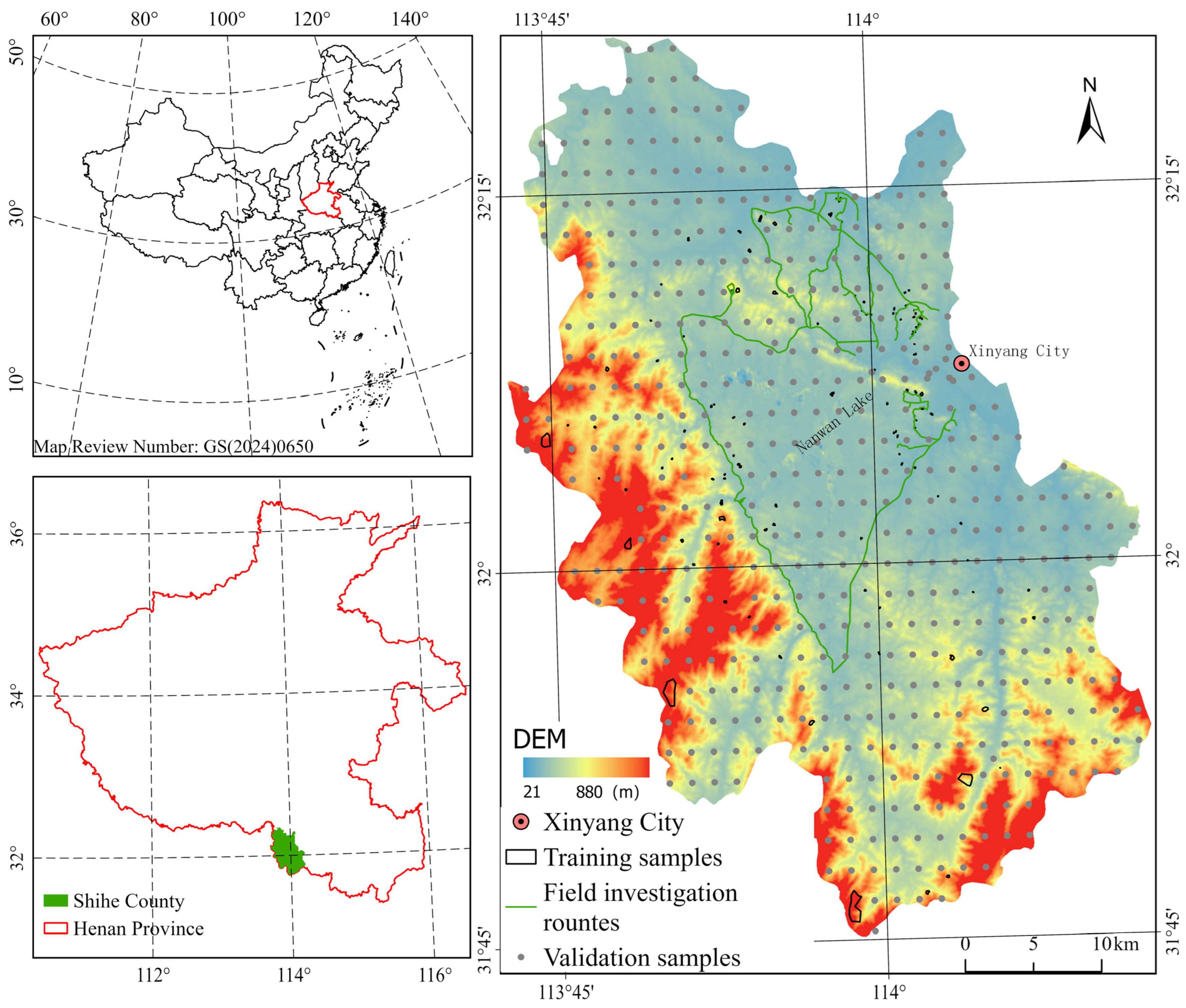
Shihe County is located in Xinyang City, Henan Province, China (approximately 32° N, 114° E) (Figure 1). The terrain is characterized by low mountains and hills, with elevations ranging from 21 to 880 m above sea level. Topographically, the area generally declines from the southwest toward the northeast. The county is situated within an ecotone transitioning from subtropical to warm-temperate monsoon climates. The region receives abundant annual precipitation, totaling approximately 1115 mm, with the majority concentrated between May and September. The area experiences four distinct seasons, with a mean annual temperature of 15.2 °C. The mean temperature in the warmest month (July) is 28 °C, while the mean temperature in the coldest month (January) drops to 2 °C.

Forests in Shihe County consist of structurally diverse stands, comprising a variety of evergreen and deciduous species. DBF dominated by Quercus variabilis and Castanea seguinii—species widely distributed in warm temperate zones—are prevalent, alongside ECF dominated by Pinus massoniana. Bamboo forests and tea plantations (Camellia sinensis) are extensively distributed in Shihe County. In addition, DCF dominated by Metasequoia glyptostroboides and EBF are extremely rare, occurring only as small-scale cultivated patches in nurseries or as landscape vegetation. Mixed forests typically exhibit DBF interspersed with ECF, bamboo, or tea plantations.

2.2. Data Sources

Sentinel-2 multispectral images and Sentinel-1 SAR images acquired during the 2022 annual cycle were downloaded from the Copernicus Open Access Hub (https://browser.dataspace.copernicus.eu/) (accessed on 20 January 2026). The Sentinel-2 constellation comprises three satellites—Sentinel-2A, Sentinel-2B, and Sentinel-2C—with the latter launched on 5 September 2024, to eventually replace Sentinel-2A. In this study, data from Sentinel-2A and Sentinel-2B were utilized. Each satellite has a revisit period of 10 days, while the combined revisit period of the two-satellite constellation is 5 days. A total of 37 Sentinel-2A/B multispectral images were obtained (

Table 1. The time information of Sentinel data. The bolded dates represent the optimal observation dates for each season.

Type	Satellites	Observation Date in 2022
SAR data	Sentinel-1A	4 May, 20 August, 31 October, 5 March
Multispectral data	Sentinel-2A	2 January, 12 January, 22 February, 3 March, 13 March, 2 April, 22 April, 2 May, 1 June, 11 June, 21 June, 11 July, 31 July, 10 August, 19 September, 29 September, 19 October, 29 October, 18 December
	Sentinel-2B	17 January, 26 February, 28 March, 7 April, 27 April, 7 May, 6 June, 16 June, 26 July, 5 August, 15 August, 25 August, 4 September, 14 September, 24 October, 3 November, 23 November, 23 December

). Sentinel-2 satellites provide freely accessible imagery with appropriate spatial, spectral, and temporal resolutions for mapping various forest attributes across large spatial scales [34]. The data comprise 13 spectral bands, including four bands at 10 m resolution (Band 2—Blue: 490 nm, Band 3—Green: 560 nm, Band 4—Red: 665 nm, Band 8—NIR1: 842 nm), six bands at 20 m resolution (Band 5—Red Edge1: 705 nm, Band 6—Red Edge2: 740 nm, Band 7—Red Edge3: 783 nm, Band 8a—NIR2: 865 nm, Band 11—SWIR1: 1610 nm, Band 12—SWIR2: 2190 nm) and three bands at 60 m spatial resolution (Band 1—Coastal Aerosol: 443 nm, Band 9—Water Vapor: 940 nm, Band 10—SWIR-Cirrus: 1375 nm) [35]. All the Sentinel-2 images were resampled into 10 m spatial resolution using the nearest-neighbor upsampling method in the Sentinel Application Platform (SNAP). For each of the four seasons, the optimal observation date was selected as the date with the least cloud cover. The representative dates for the spring, summer, autumn, and winter were determined as 2 May, 15 August, 3 November, and 3 March, respectively.

The 5-day revisit cycle of Sentinel-2 enables frequent acquisition of land surface information over a given period. Since the normalized difference vegetation index (NDVI) has been demonstrated to be a reliable indicator of multiple vegetation parameters, including leaf area index, greenness, biomass, and metabolic activity [36], it was selected to capture the phenological differences among vegetation types. Accordingly, an NDVI time series for 2022, capturing fine-scale details of vegetation growth across different tree species, was generated for Shihe County using Sentinel-2 data, with the aim of enhancing forest type classification performance. Specifically, a total of 37 Sentinel-2 images, which were geometrically and radiometrically calibrated, were first used to calculate NDVI in SNAP. Concurrently, the corresponding quality cloud confidence bands were extracted and resampled to 10 m using the nearest-neighbor method. Pixels with a value greater than 20 in the cloud confidence band were identified as being significantly affected by clouds or cloud shadows, and the corresponding NDVI values were replaced with those from temporally adjacent images through linear interpolation. Subsequently, the maximum value composite (MVC) method was adopted to generate 10-day composite images. Additionally, gaps in the images caused by prolonged rainy weather were filled using nearest-neighbor temporal interpolation to produce a complete time series at a 10-day temporal resolution. Finally, the 10-day NDVI time series were reconstructed using the Savitzky–Golay filter to reduce residual noise while preserving true vegetation phenological dynamics. The window size and the number of envelope iterations were set to 4 and 1, respectively, and a median filter was employed for spike removal.

The Sentinel-1 constellation comprises two satellites—Sentinel-1A and Sentinel-1B, equipped with C-band SAR sensors. The primary acquisition mode for terrestrial applications is the interference wide (IW) model. Ground range detected (GRD) products from Sentinel-1A were utilized in this study. Four Sentinel 1A SAR images corresponding to, or nearest to, the optimal observation dates of the four seasons were also downloaded (Table 1). The downloaded data were preprocessed in SNAP, which included geometric correction, thermal noise removal, radiometric calibration, speckle noise filtering, and terrain correction. The processed data were then converted from a linear scale to a decibel scale to obtain backscattering coefficients. We thus obtained backscattering intensity data, including VV and VH polarization data at 10 m resolution, for the four seasonal windows, which characterize vegetation structure and type-related features.

2.3. Methods

2.3.1. The Processes for Classification

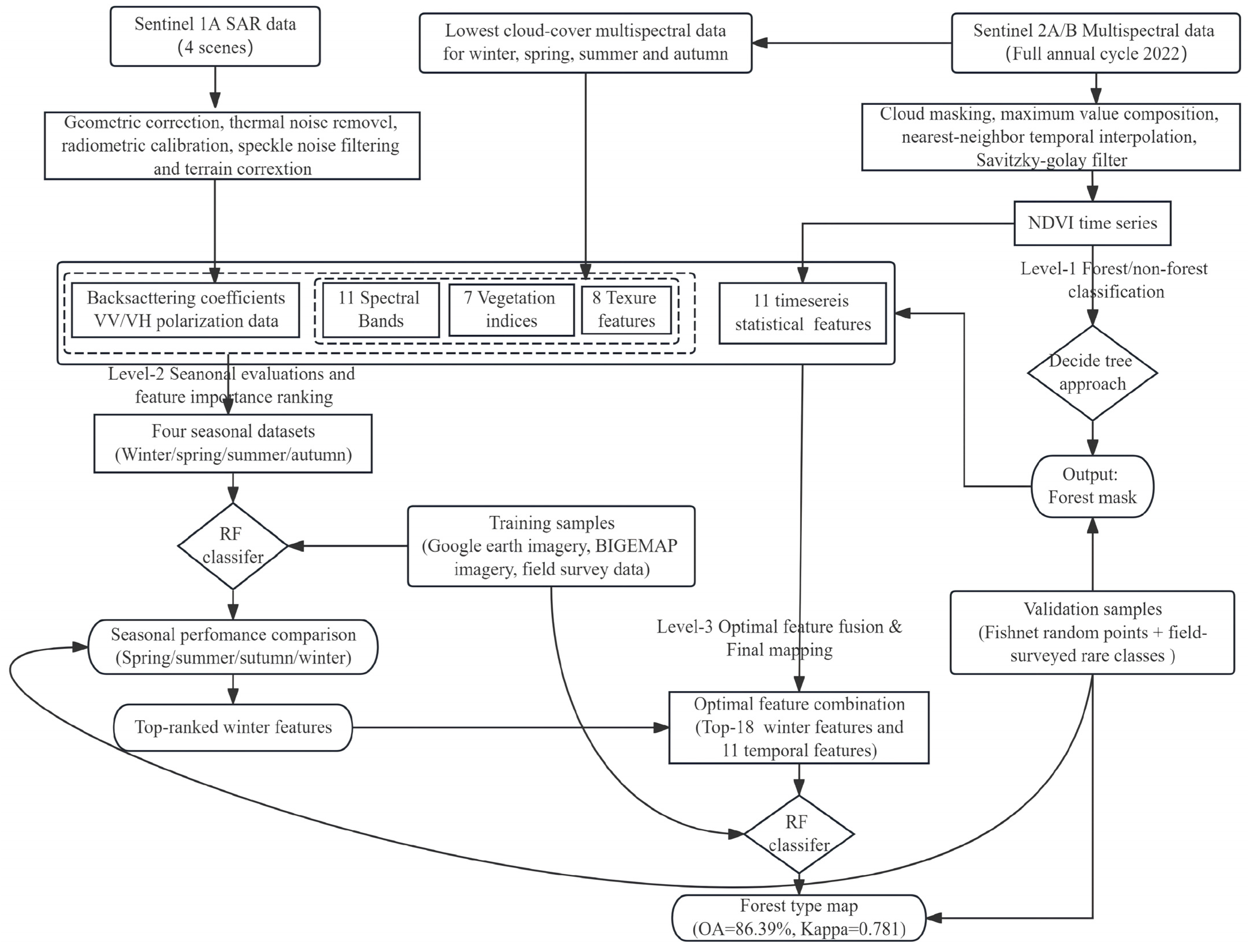
This study developed a three-level hierarchical classification framework designed to classify the landscape into forest and non-forest areas, and further into different forest types (Figure 2).

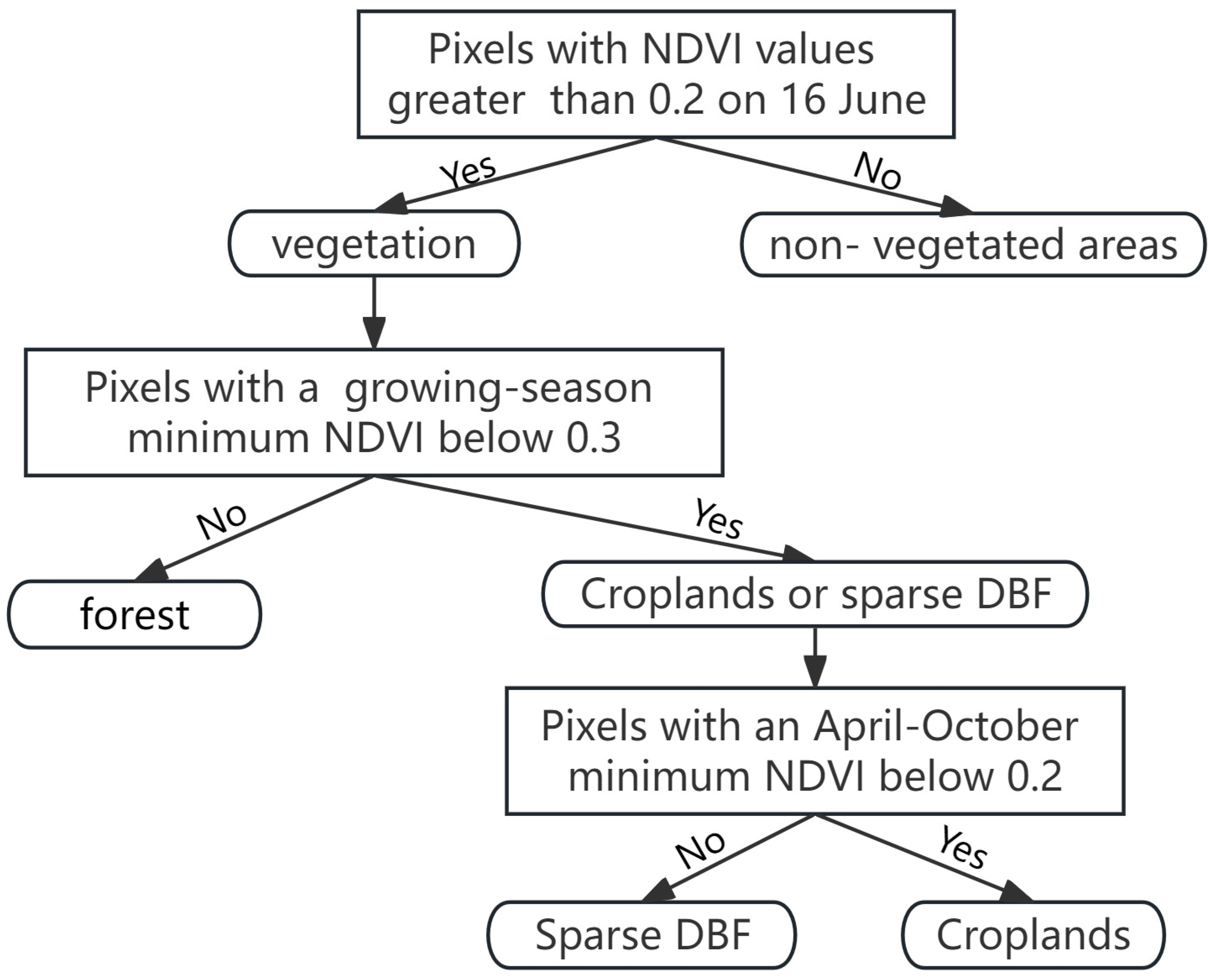
At the first level, most non-forest backgrounds were excluded from subsequent processing using a rule-based decision tree approach (Figure 3). Generally speaking, non-vegetated surfaces typically show an NDVI value less than 0.2 [36]. Vegetated areas were initially distinguished from non-vegetated surfaces using summer (peak growing season) NDVI data with a threshold exceeding 0.2. Therefore, the NDVI image on 16 June (a clear summer observation date) was first used to remove the non-vegetated pixels. To further discriminate forests from croplands and sparse DBF, the minimum NDVI values during the growing season (March to November) were examined. Given that croplands exhibit pronounced seasonal NDVI troughs due to harvesting or sowing, and considering the effects of fragmented plots and field ridges, a combined exclusion criterion was applied: pixels with a growing-season minimum NDVI below 0.3, in addition to those with an April-to-October minimum NDVI below 0.2, were classified as non-forest. Consequently, the decision tree results were binarized into forest (encompassing both forest and sparse DBF in Figure 3) and non-forest categories.

At the second level of classification, a dataset comprising 28 features for each season was assembled based on the original Sentinel-2 spectral bands, derived VIs, texture features, and backscattering coefficients acquired on the optimal dates of the four seasons (

Table 2. Detailed information on the features adopted for forest type classification in four seasons.

Type	Name	Details
Bands	B2, B3, B4, B5, B6, B7, B8, B8a, B9, B11, B12,	Sentinel-2 A/B
VIs	RVI	B8/B4
	MVI	(B8 − B5 − B11)/(B8 + B5 + B11)
	NDVI	$(\mathrm{B}8-\mathrm{B}4)/(\mathrm{B}8+\mathrm{B}4)$
	NDRI	$(\mathrm{B}8-\mathrm{B}5)/(\mathrm{B}8+\mathrm{B}5)$
	NDWI	$(\mathrm{B}2-\mathrm{B}8)/(\mathrm{B}2+\mathrm{B}8)$
	SNIR	B6 + B7 + B8 + B8a + B9
	MSAVI	0.5 × {2 × B8 + 1 − sqrt[square(2 + B8 + 1) − 8 × (B8 − B4)]}
Texture features	Mean	Computed from band B8 using GLCM
	Contrast
	Entropy
	Variance
	Correlation
	Dissimilarity
	Homogeneity
	Second moment
Backscattering coefficients	VV	Derived from Sentinel-1 SAR data
	VH

). The RF classifier—capable of efficiently processing high-dimensional data and exhibiting strong robustness against overfitting—was then applied to evaluate the performance of the four seasonal datasets. Furthermore, the Gini importance metric, implemented within the RF classifier, was employed to quantify the relative contribution of each feature to the classification.

The RF algorithm, proposed by Breiman [37], is an ensemble learning method based on classification and regression trees (CART). It operates by generating a large number of decision trees during training, with each tree constructed from a bootstrap sample of the original training data and a randomly selected subset of predictor variables at each node. RF efficiently handles high-dimensional data, exhibits strong noise resistance and nonlinear modeling capability, and is particularly effective when combined with multiple features, as it captures complex inter-feature relationships through ensemble decision-making. The final classification outcome is determined by majority voting across all decision trees, yielding high accuracy and robust generalization performance. These advantages make RF well-suited for vegetation classification tasks that require the integration of multi-source remote sensing data [25,38]. In this study, RF was implemented using the ENVI platform (version 5.6). The number of trees was set to the default value of 100, and the minimum leaf node size was set to 1. Furthermore, the RF algorithm internally computed feature importance scores based on the Gini impurity criterion. Through feature importance ranking, the algorithm identifies the variables contributing most significantly to classification accuracy, thereby optimizing the model and enhancing predictive performance. Based on this ranking, the most influential features for forest type classification in the study area were subsequently determined.

At the third classification level, we first evaluated the performance of multi-feature fusion on classification accuracy by testing various feature group combinations using the optimal seasonal dataset. To reduce data redundancy and identify the most informative features, we individually tested the optimal feature group combination and several top-ranking feature subsets—each augmented with the 11 temporal features—using the RF classifier to determine the best-performing set for the final forest type mapping of Shihe County.

2.3.2. Datasets for Forest Type Classification

Seven VIs—namely, the NDVI, the normalized difference water index (NDWI), the modified vegetation index (MVI), the normalized difference red-edge index (NDRI), the ratio vegetation index (RVI), the modified soil-adjusted vegetation index (MSAVI), and the sum of near-infrared reflectance (SNIR)—were derived from the spectral reflectance of the corresponding bands for each of the four seasons (Table 2). To enhance the spectral separability between bamboo forest and other evergreen forest types, the MVI was modified by replacing the originally red band with the red-edge 1 band, a Sentinel-2 specific spectral band [29]. Eight texture features—namely, the mean, variance, homogeneity, contrast, dissimilarity, entropy, second moment, and correlation—were computed from the NIR1 band (B8) using the gray-level co-occurrence matrix (GLCM) for the same seasonal periods. To better characterize structural heterogeneity among forest types, texture features were extracted with a 3 × 3 sliding window and quantified at 64 gray levels. In total, a total of 28 features per season—comprising 11 spectral bands, 7 VIs, 8 texture features, and 2 backscattering coefficients—were employed to evaluate their performance of single-date datasets for forest type classification.

Based on the phenological growth characteristics of the dominant forest types in the study region, 11 statistical features (

Table 3. Statistical features derived from the reconstructed 2022 NDVI time series.

ID	Feature Name (Brief)	Equation
F1	Annual range	max(NDVI_year) − min(NDVI_year)
F2	Spring range	max(NDVI_Mar–May) − min(NDVI_Mar–May)
F3	Summer range	max(NDVI_Jun–Aug) − min(NDVI_Jun–Aug)
F4	Autumn range	max(NDVI_Sep–Nov) − min(NDVI_Sep–Nov)
F5	Winter range	max(NDVI_Dec–Feb) − min(NDVI_Dec–Feb)
F6	January peak	max(NDVI_Jan)
F7	March range	max(NDVI_Mar) − min(NDVI_Mar)
F8	Greening variability	F2 − F7
F9	Senescence sum	∑(NDVI_i) for i = DOY 271 to 321
F10	Browning variability	F4 − F5
F11	Winter-summer diff	NDVI_Mar 3 − NDVI_Jun 16

) derived from the reconstructed NDVI time series and incorporated into the feature set for the third-level classification (Section 2.3.1). These metrics encompassed general phenological indicators, including the annual NDVI range (annual range), seasonal NDVI ranges for spring, summer, autumn, and winter (namely, spring range, summer range, autumn range, winter range, respectively), and the maximum NDVI value during the coldest month (January peak). In addition, features characterizing the spring green-up period (primarily March and April) and the autumn senescence phase (primarily October and November) were also considered. Accordingly, several specific features were added to the dataset: the NDVI range in March (March range), the difference between the March range and the March–May range (representing greening variability), the cumulative NDVI between October and November (the senescence sum), and the difference between the autumn and winter ranges (representing browning variability).

Among all evergreen vegetation, tea plantations generally exhibit higher NDVI values in winter compared to other forest types, but lower values in June owing to management practices such as pruning. Accordingly, the NDVI difference between 3 March and 16 June (namely, the winter-summer diff in Table 3) was employed as a discriminating feature to separate tea plantations from evergreen forest types. Finally, all the data were standardized and reprojected to the WGS 84/UTM zone 49N coordinate system to ensure geometric consistency.

2.3.3. The Sampling Strategy

The availability of representative training samples is fundamental to the accuracy of supervised classification. In this study, training samples were collected based on high-resolution winter imagery from the BIGEMAP platform (http://www.bigemap.com/) (accessed on 1 August 2025) and were subsequently validated through historical imagery in Google Earth and comprehensive field surveys (Figure 1). A total of 115 patches were collected (

Table 4. Statistics of the training and validation samples.

Type	Training Samples		Validation Samples
	Number of Patches	Area (m2)	Number
DBF	16	4,278,357	207
ECF	16	297,439	14
Bamboo forest	28	134,319	36
EBF	7	14,800	7
DCF	3	6536	5
Tea plantations	37	341,586	44
OL	8	50,912	46
Non-forest	0	0	103
Total	115	5,139,386	462

), comprising 16 classified as DBF, 16 as ECF, 28 as bamboo forest, 7 as EBF, 3 as DCF, 37 as tea plantations, and 8 as other land (OL, mainly abandoned croplands). The same training samples were consistently applied to the second- and third-level forest type classification (Figure 2).

A total of 900 random points were generated using a 30 × 30 fishnet grid in ArcGIS Pro (version 3.5.2); of these, 488 points were located within Shihe County. After removing points that fell inside or adjacent to the training sample patches (a distance of 500 m buffer), 456 points were retained. Land cover types for the remaining points were interpreted using high-resolution historical imagery available in Google Earth, based on criteria including winter leaf-off conditions, textural characteristics, seasonal phenology, temporal dynamics, and spatial associations with houses. Excluding three unidentifiable points, the interpreted samples (453 points) comprised 207 classified as DBF, 14 as ECF, 36 as bamboo forest, 2 as EBF, 1 as DCF, 44 as tea plantations, 46 as OL, and 103 as non-forest land. To supplement the validation set, an additional five EBF and four DCF derived from prior field surveys were incorporated, yielding a total of 462 validation samples (Table 4). A confusion matrix was constructed using all accuracy assessment points, from which four metrics—overall accuracy (OA), kappa coefficient, user accuracy (UA), and producer accuracy (PA)—were calculated to evaluate the classification accuracy.

3. Results

3.1. Classification of Forest and Non-Forest Types

The forest/non-forest classification derived from the decision tree approach was validated using the 453 interpreted samples obtained from fishnet-based random sampling. The validation results yielded an OA of 98.90% and a kappa coefficient of 0.968 (

Table 5. Confusion matrix of forest/non-forest classification using the decision tree algorithm.

	Non-Forest	Forest	Total	UA (%)
Non-forest	100	2	102	98.04
Forest	3	348	351	99.15
Total	103	350	453
PA (%)	97.09	99.43		98.90

). The PA and UA for the forest class were 99.43% and 99.15%, respectively, while those for the non-forest class were 97.09% and 98.04%, respectively. Classification errors were primarily attributed to abandoned croplands being misclassified as forest, largely because abandoned croplands exhibit phenological trajectories highly similar to those of DBF. To mitigate this issue and improve classification accuracy in the subsequent second- and third-level classifications, an additional class—OL—was incorporated into the training sample set alongside the six forest types.

3.2. Optimal Classification Season and Feature Importance for Forest Type Classification

The second- and third-level forest type classifications were validated using the sample points that had been identified as forest in the first-level classification. A total of 360 points, including the three misclassified points in the first-level classification, were retained to evaluate the performance of the feature subsets. Classification accuracy varied substantially across seasons (

Table 6. Classification accuracy of forest types across four seasons.

	OL		ECF		EBF		Bamboo Forest		Tea Plantation		DCF		DBF
	PA	UA	PA	UA	PA	UA	PA	UA	PA	UA	PA	UA	PA	UA	QA	Kappa
Spring	26.09	66.67	50	35	0	0	58.33	28.77	48.84	45.65	40	50	76.70	81.03	61.39	0.402
Summer	13.04	35.29	50	46.67	14.29	20	30.56	20.75	48.84	48.84	40	100	80.58	73.78	59.44	0.33
Autumn	52.17	55.81	28.57	30.77	28.57	66.67	16.67	50	44.19	82.61	40	100	92.23	71.97	68.61	0.432
Winter	50	65.71	78.57	84.61	28.57	40	80.56	43.94	58.14	71.42	20	50	84.95	85.78	73.89	0.587

). The winter dataset achieved an OA of 73.89% (kappa = 0.587), substantially outperforming autumn (68.61%, kappa = 0.432), spring (61.39%, kappa = 0.402), and summer (59.44%, kappa = 0.33). Overall, when integrating multi-feature data for a single temporal phase, the classification accuracy for forest types followed the order: winter > autumn > spring > summer. Late winter was identified as the optimal observation period for forest type classification in Shihe County, indicating that the spectral differences among forest types are most pronounced during this period. DBF consistently achieved the highest classification accuracy, with PA and UA exceeding 70% across all four seasons. However, the high UA (100%) observed for DCF in summer and autumn should be interpreted with considerable caution, owing to its limited occurrence in the study area and the small number of validation samples (5 for DCF). Overall, these results demonstrated that not all forest types can be effectively distinguished using a single-date Sentinel data alone.

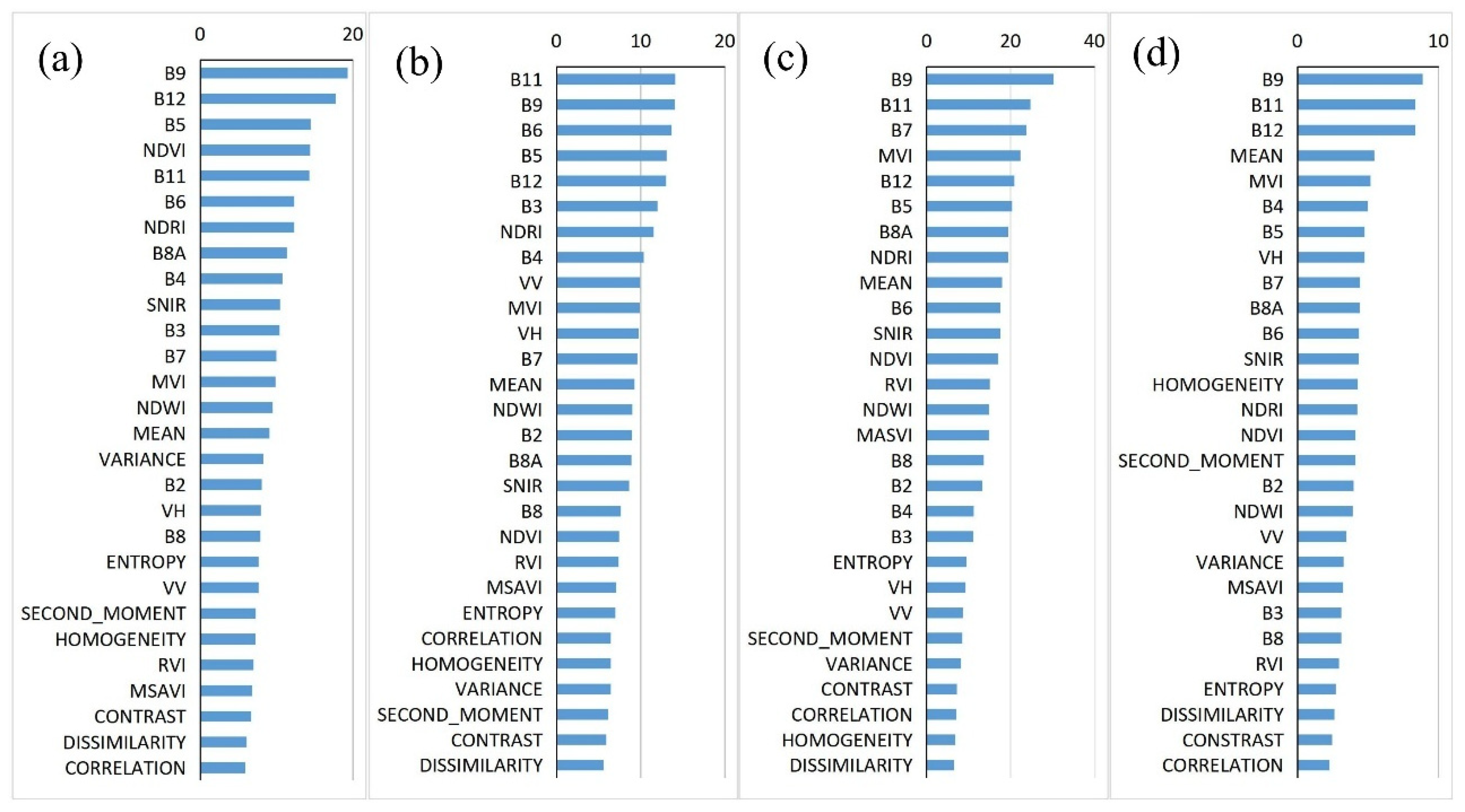
Feature importance was assessed using the Gini importance ranking embedded in the RF classifier (Figure 4). Across all seasons, the original spectral bands—particularly B9, B11, and B12, and the red-edge bands (B5, B6, B7)—consistently ranked among the most influential variables for forest type classification. Among the seven VIs, the NDVI was relatively low importance in all seasons except spring (Figure 4a). In contrast, the MVI and NDRI maintained consistently high rankings across all seasons, underscoring the critical role of red-edge information in discriminating forest types. The SNIR also exhibited moderate to high importance in all seasons except summer (Figure 4b). Texture features were most substantially to the classification accuracy in winter, whereas their importance diminished in the other seasons, likely due to the generally dense and homogeneous vegetation cover during the growing periods. Among the eight GLCM-derived texture features, the mean texture feature was consistently the most important, while correlation, contrast, dissimilarity, and entropy consistently received the lowest importance scores across all seasons. Regarding SAR backscattering, polarization data were more influential in summer and winter, but showed negligible importance in spring and autumn (Figure 4c). Generally, VH polarization outperformed VV polarization in all seasons other than summer (Figure 4b). In winter, the most informative features were identified as spectral bands, the mean texture feature, MVI, SNIR, and VH-polarized backscatter (Figure 4d).

3.3. Optimal Feature Fusion for Winter Forest Type Classification

To assess the influence of different feature groups on winter classification performance, we constructed multiple datasets with varied feature combinations, and summarized their OA and kappa coefficients in

Table 7. Classification accuracy of different feature group combinations for winter forest type mapping.

Scheme	Feature Set	No. of Features	OA (%)	Kappa
1	Bands	11	73.61	0.598
2	Bands + Textures	19	73.89	0.599
3	Bands + Backscattering	13	69.72	0.539
4	Bands + VIs	18	75.28	0.617
5	Bands + VIs + Textures	26	75.56	0.625
6	Bands + VIs + Backscatter	20	73.06	0.585
7	Bands + Textures + Backscattering	21	71.39	0.557
8	Bands + VIs + Textures + Backscattering	28	73.89	0.587
9	Bands + VIs + Textures + VH	27	75.28	0.611

. Classification using only spectral bands (Scheme 1) achieved an OA of 73.61%. Scheme 2 and Scheme 4 both outperformed Scheme 1, with Scheme 5 yielding the highest accuracy among all multi-feature schemes. These results indicate that VIs and texture features both enhance multispectral classification, with VIs contributing more substantially than textures. The addition of eight texture features to Scheme 2 and Scheme 5 produced only a slight accuracy gain. Conversely, incorporating backscattering coefficients generally reduced accuracy (Scheme 3 vs. Scheme 1, Scheme 6 vs. Scheme 4, and Scheme 8 vs. Scheme 5). However, the inclusion of a single VH polarization channel resulted in a slight accuracy loss (Scheme 9 vs. Scheme 5).

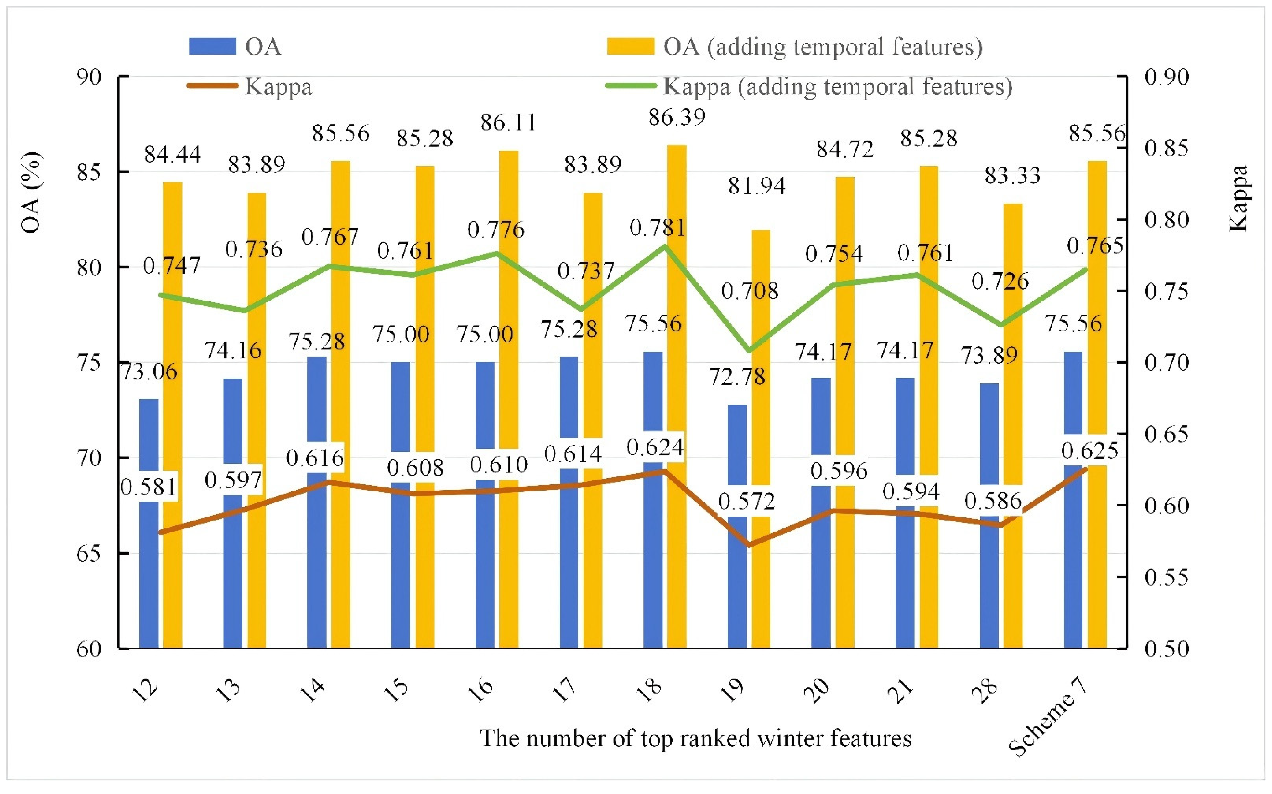
To mitigate the effects of data redundancy and overfitting on classification performance, we evaluated incremental subsets of the top-ranked features derived from the winter importance ranking (Figure 4d) and assessed their corresponding classification accuracies (Figure 5). The subset comprising the top 12 features—covering all four feature types—yielded an OA of 73.06%, while the top-18 feature subset achieved the highest accuracy, matching that of the full Scheme 7 combination. Notably, the top-15 subset produced a lower accuracy than the top-14 subset. Similarly, the top-19, top-20, and top-21 subsets all yielded lower accuracies than the top-18 subset. These results further confirm the presence of redundancy within the winter dataset.

As shown in Figure 5, incorporating 11 temporal features significantly improved OA by approximately 10% across all subsets relative to their counterparts without such features. The integrated dataset combining Scheme 7 and the 11 temporal features achieved an OA of 85.56%. When the top 14, top 16, and top 18 winter-ranked features were respectively combined with the 11 temporal features, their classification accuracy always exceeded that of the Scheme 7 + temporal features combination. Classification accuracy peaked when the top 18 winter-ranked features were combined with the 11 temporal features, yielding a 10.83% improvement in OA over the top-18 winter subset alone. Accordingly, the optimal feature set—comprising the top 18 features from the winter importance ranking and the 11 temporal statistical features—was selected for final forest type mapping in Shihe County.

3.4. Forest Type Mapping in Shihe County Using the Best-Performing Winter Dataset

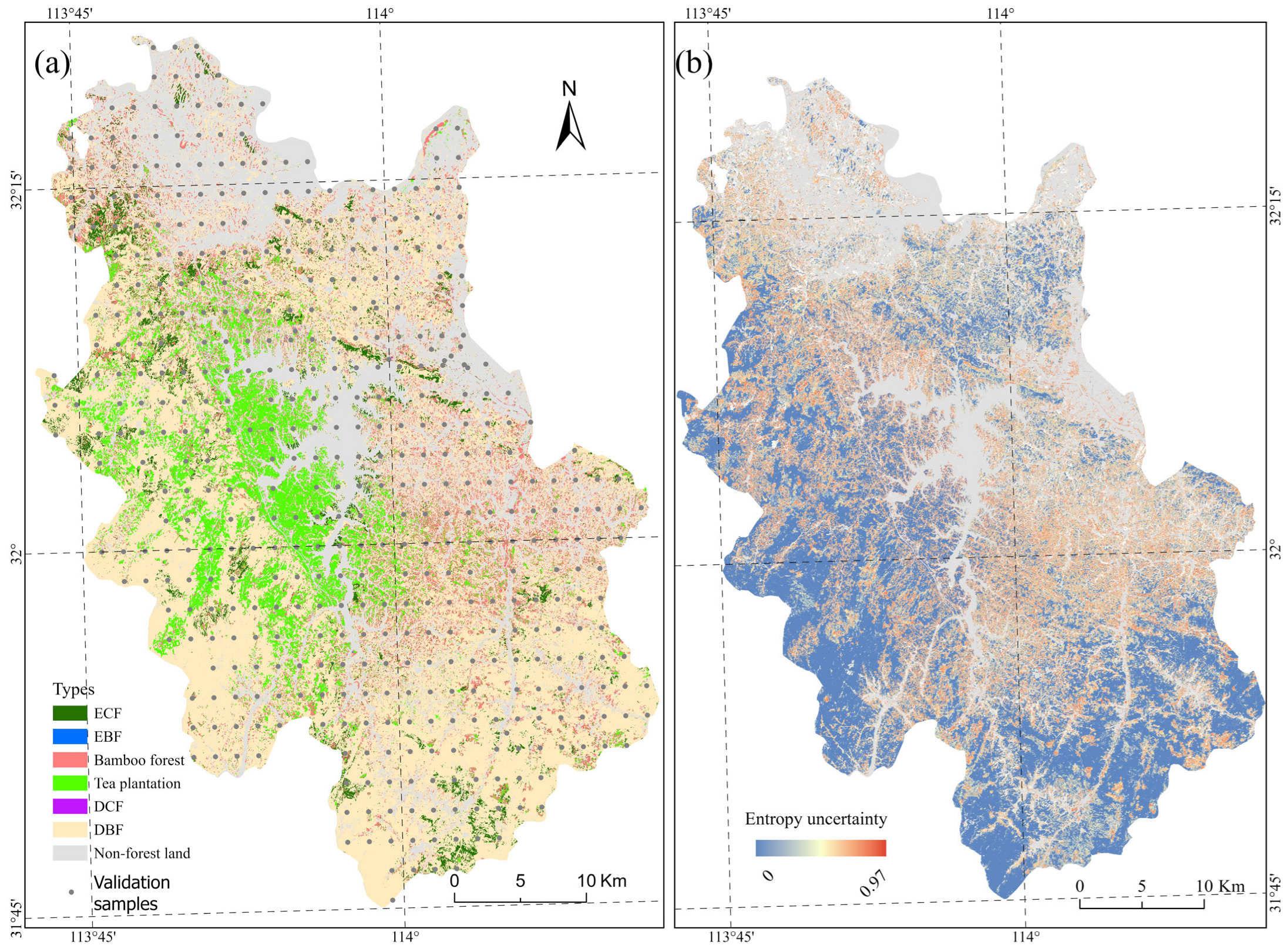
Using the RF classifier with the optimal dataset—comprising the top 18 features from the winter importance ranking and the 11 temporal statistical features—the OA and kappa coefficient reached 86.39% and 0.781, respectively (

Table 8. Confusion matrix of forest type classification in Shihe County. The OA and kappa coefficients account for error propagation from the first-level forest and non-forest classification to this stage.

	OL	ECF	EBF	Bamboo Forest	Tea Plantations	DCF	DBF		UA (%)
OL	33	0	1	0	0	0	8	42	78.57
ECF	0	12	0	0	2	0	0	14	85.71
EBF	1	0	5	0	0	0	0	6	83.33
Bamboo forest	4	0	2	34	15	0	1	56	60.71
Tea plantations	0	0	0	0	26	0	0	26	100
DCF	0	0	0	0	0	4	0	4	100
DBF	8	2	0	2	0	1	197	212	92.92
	46	14	7	36	43	5	206	360
PA (%)	71.74	85.71	71.43	94.44	60.47	80	95.63		86.39

). Major forest types in Shihe County, including DBF, ECF, and DCF, achieved relatively high classification accuracies, meeting the requirements for reliable forest type identification. The PA and UA of OL were relatively low (71.74% and 78.57%, respectively), indicating that distinguishing between DBF from abandoned croplands remains a challenging task requiring future investigation. Additionally, bamboo forest exhibited a relatively low UA of 60.71%, while tea plantations showed a notably low PA of 60.47%, due to a considerable misclassification between those two cover types. Specially, 15 validation samples of tea plantations were misclassified as bamboo forest (Table 8). The classification of EBF and DCF is subject to considerable uncertainty owing to the limited sample size available for the two classes.

The total forest area in Shihe County (including tea plantations) is 1304.79 km², covering 59.45% of the total land area. Among the forest types, DBF, bamboo forest, tea plantations, ECF, and EBF account for 68.223%, 14.107%, 11.815%, 5.469%, and 0.385% of the forest area, respectively (

Table 9. Area and proportion of each forest type in Shihe County, based on pixel-count statistics from the RF classification using the optimal feature set. Note: values are derived from classified map pixels and represent mapped areas, not unbiased area estimates.

Type	Area (km2)	Proportion of Forest Area (%)
DBF	890.16	68.223
Bamboo forest	184.06	14.106
Tea plantations	154.16	11.815
ECF	71.35	5.469
EBF	5.02	0.385
DCF	0.03	0.002
Total	1304.79	100

). The forest landscape in Shihe County is predominantly composed of DBF, with a considerable proportion of characteristic subtropical resources such as bamboo and tea plantations, followed by ECF. In contrast, EBF and DCF are extremely limited in this transitional zone. Spatially, DBF is widely distributed, with concentrations in the western and southeastern mountainous areas (Figure 6a). Tea plantations are mainly concentrated on the western side of Nanwan Lake, extending toward the southwestern mountains and the eastern side of the lake. Bamboo is primarily found in the eastern hilly region, occurring as patches near residential areas. ECF is mainly distributed on high hilltops. There were notable differences in classification confidence across the county based on the normalized entropy-based uncertainty (Figure 6b). Areas with higher uncertainty were concentrated primarily along patch edges and transition zones between land cover types, with the most pronounced uncertainty observed on the eastern and northwestern sides of Nanwan Lake. These regions are characterized by fragmented forest patches and complex land cover types.

4. Discussions

4.1. Optimal Season for Forest Type Classification

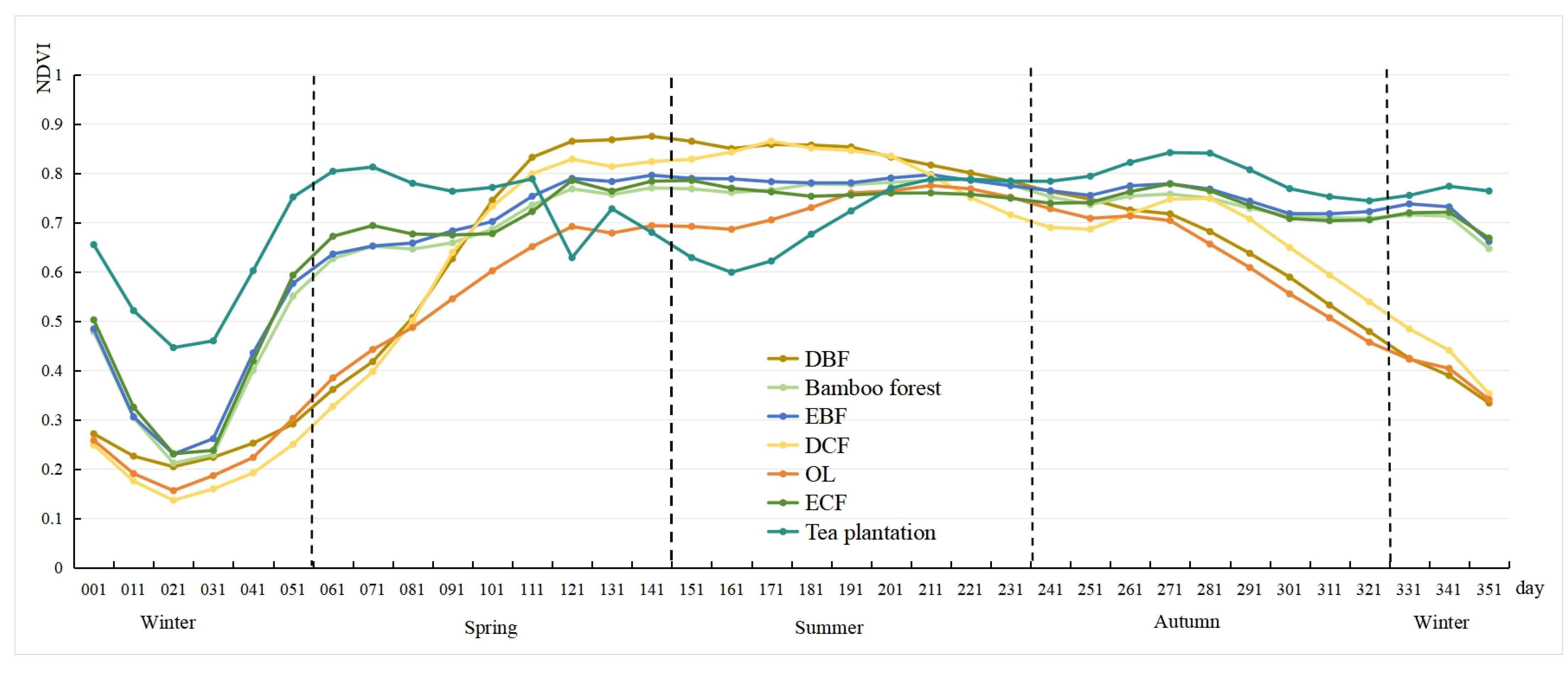
The spectral properties of different forest types vary significantly with phenological phase, crown closure, growth stage, and observation conditions. The optimal classification season is region-dependent. For example, late-spring and mid-summer imagery performed well for species-level classification in the Changbai Mountain region of Northeast China [39]. In this study, we characterized the 10-day NDVI dynamics of major forest types in Shihe County throughout 2022 (Figure 7). The NDVI time-series curves revealed substantial inter-type differences. Overall, NDVI values varied among forest types diverged most markedly in late winter and early spring—particularly among tea plantations, deciduous forests, and evergreen forests—while differences were minimal in summer. This seasonal pattern aligns with our finding that late winter (3 March, corresponding to approximately day 61 in Figure 7) constitutes the optimal seasonal window for forest type classification, whereas summer (15 August, approximately day 221) yielded the lowest classification accuracy. As for Shihe County, deciduous vegetation (DBF and DCF) is in a leafless state in late winter, while evergreen forests (EBF, ECF, and bamboo forest) and tea plantations remain photosynthetically active, resulting in pronounced spectral and phenological differences during this period [40]. Moreover, owing to physiological characteristics and management practices (e.g., fertilization), local tea plantations exhibit significantly higher NDVI values in winter than other evergreen forests [41]. Consequently, forest type classification accuracy during the late winter and early spring period reached its highest level in this study. This finding aligns with previous observations in subtropical regions [42].

4.2. Multi-Feature Fusion Is of Great Importance for Forest Type Classification

Several classification experiments were conducted using datasets that integrated spectral bands, VIs, texture features, backscattering coefficients, and time-series statistical features to discriminate forest types in Shihe County. The integration of multispectral bands, VIs, texture features, and temporal features yielded an OA of 85.56% (kappa = 0.765) (Figure 5). Our results confirm that multi-feature fusion substantially benefits for discriminating forest types, providing a more comprehensive and reliable approach that is consistent with previous findings [43,44]. Vegetation indices proved effective for discriminating forest types in this study, (e.g., Scheme 4 vs. Scheme 1, and Scheme 8 vs. Scheme 7 in Table 7). Texture features have been shown to improve OA by approximately 2% in medium-resolution images [19,45], and their contribution is typically greater when derived from high-resolution data than from medium-resolution data. In this study, however, the eight texture features led to only a slight improvement in classification accuracy when combined with multispectral bands and VIs, or both of them (Scheme 2 vs. Scheme 1, and Scheme 5 vs. Scheme 4). Similarly, several texture features consistently ranked low across all seasons (Figure 4). The inclusion of temporal features significantly enhanced classification performance by approximately 10% in this study. This is consistent with prior work showing that using satellite scenes from different phenological periods yields significantly better results than using a single scene [46,47], with reported OA improvements ranging from 10% [48] to as high as 28% [49]. Regarding backscattering coefficients, the added SAR data led to a decline in both OA and kappa (Schemes 3, 6, and 7). The reasons for this decline merit further investigation. Topographic variables—particularly elevation, which is strongly correlated with temperature—play an important role in species distribution and growth, and have been shown to improve forest classification accuracy in mountainous regions [20,50]. The addition of topographic features such as slope, profile convexity, and minimum curvature has been reported to increase OA by approximately 3% [39,49]. Nevertheless, it should be noted that topographic features were not included in the present study.

4.3. The Important Features for Improving Forest Type Classification

Our results confirmed the importance of original spectral bands across all four seasons, with shortwave infrared (SWIR) bands being the most influential features in winter—a finding consistent with previous studies [45]. VIs also proved valuable for forest type discrimination. Although the NDVI has been shown to be effective for distinguishing eight forest types [19] and served as a key predictor in spring, it was consistently outranked by MVI, NDRI, and SNIR in the remaining seasons (Figure 4). This may be attributable to redundant information conveyed by the near-infrared band in our dataset. The prominent performance of MVI and NDRI underscores the critical role of red-edge features in forest discrimination. Among the eight texture features derived from the near-infrared band, the mean texture feature was the most important across all seasons, particularly in winter. In contrast, correlation, dissimilarity, contrast, and entropy consistently ranked among the least influential features throughout the year. Regarding backscattering coefficients, SAR data contributed minimally to forest type discrimination in spring and autumn. However, VV-polarized data exhibited relatively high importance in summer, whereas VH-polarized data ranked highly in winter. This seasonal divergence aligns with earlier findings that different forest types exhibit greater separability in VH-polarization signals than in VV-polarization signals [38,51].

The selection of suitable variables is a prerequisite for improving classification accuracy. Although the integration of ancillary data with conventional spectral classification can enhance performance, the incremental benefit of additional features often becomes negligible—or even detrimental—beyond a certain dataset size. To mitigate this issue, we demonstrated that removing unimportant features can effectively improve classification accuracy. For winter classification incorporating temporal features, the dataset composed of the top 14 ranked features achieved higher accuracy than the dataset based on the optimal feature group combination dataset (37 variables) (Figure 5). Similarly, the top-18 feature subset outperformed the top-20 feature subset. These results suggest that increasing the number of features does not necessarily improve accuracy and may even reduce it. Nevertheless, the optimal selection and combination of features—which cannot be accomplished by RF importance ranking alone—remains a persistent challenge in forest type classification.

4.4. Limitations of the Study and Future Research Directions

Finally, several limitations of this study should be acknowledged. First, our analysis focused on the major forest types in Shihe County. However, the classification accuracy for certain forest types—particularly the typical subtropical EBF and the regionally sparse DCF—is subject to considerable uncertainty, owing to the limited number of training and validation samples for these classes. Consequently, future studies should extend the spatial extent to a larger region that encompasses more representative occurrences of these forest types, so as to reduce classification uncertainty and improve statistical robustness.

Second, although a set of remote sensing variables was employed in this study for forest type discrimination, numerous potentially effective features—such as the enhanced vegetation index (EVI), topographic features, and tasseled cap transformation components—remain to be explored. The selection and systematic evaluation of remote sensing parameters is a key issue in similar studies. In the present study, the discrimination accuracy between bamboo forests and tea plantations still requires further improvement, because mixed forests composed of DBF and tea plantations, as well as newly established tea plantations that often replace existing bamboo forests, are frequently misclassified as bamboo forest. Therefore, key remote sensing parameters that can effectively characterize or discriminate these two vegetation types need to be investigated to enhance their separability.

Third, we confirmed that feature selection and optimal feature combination are necessary to achieve robust and efficient forest type classification. It should be recognized that the feature importance derived from RF does not reveal causal relationships between predictor variables and classification outcomes. We plan to adopt model interpretability methods—such as attention mechanisms (AM), Shapley additive explanations (SHAP), and local interpretable model-agnostic explanations (LIME)—which can provide global or local explanations by quantifying feature contributions. Furthermore, it should be noted that all model optimization procedures were carried out exclusively on the polygon-based training dataset and evaluated using the point-based validation samples in this study. To reduce overfitting and improve model transferability, future studies should compile a spatially representative training dataset and adopt spatial cross-validation strategies for more robust model selection [52]. These techniques will facilitate the identification of robust and universally applicable remote sensing parameters for forest type discrimination.

5. Conclusions

By integrating multi-feature datasets—including spectral bands, VIs, texture features, backscattering coefficients, and time-series statistical features—derived from Sentinel-1 SAR and Sentinel-2 multispectral data, we employed a multi-level RF-based classification framework to map the major forest types in Shihe County. This approach is transferable to areas with similar biophysical settings, as almost all features are generated objectively, circumventing manual operations such as threshold selection. Our findings revealed that spectral separability in Shihe County peaked in late winter and early spring (3 March), establishing this period as the optimal period for forest cover type classification. DBF achieved relatively high classification accuracy across all seasons.

The SWIR and red-edge bands, MVI, NDRI, mean texture feature, and VH-polarized backscattering coefficient were identified as influential variables for forest type discrimination. Among all winter schemes, the combination of spectral bands, VIs and texture features yielded the highest classification accuracy. The addition of time-series statistical features further improved classification performance, increasing OA by approximately 10%. Nevertheless, to identify the critical features for discriminability among forest types, feature selection or optimization of feature combinations remains necessary. The optimal feature set—comprising the top 18 winter-ranked features and the 11 temporal features—achieved the highest classification performance, with an OA of 86.39% and a kappa coefficient of 0.781. Misclassification between bamboo forests and tea plantations was the primary factor limiting further improvement in classification accuracy; future studies should extend the spatial extent to a larger region that encompasses more representative occurrences of EBF and DCF. In terms of land cover composition, DBF dominated Shihe County, while evergreen forests occupied 31.78% of the forestland. This composition clearly reflects the transitional ecological characteristics of this region.

References

1. Yu, Z.; Ciais, P.; Piao, S.; Houghton, R.A.; Lu, C.; Tian, H.; Agathokleous, E.; Kattel, G.R.; Sitch, S.; Goll, D.; et al. Forest expansion dominates China’s land carbon sink since 1980. Nat. Commun. 2022, 13, 5347. [Google Scholar] [CrossRef] [Scilit] [PubMed]
2. Laurin, G.V.; Puletti, N.; Hawthorne, W.; Liesenberg, V.; Papale, D.; Chen, Q. Discrimination of tropical forest types, dominant species, and mapping of functional guilds by hyperspectral and simulated multispectral Sentinel-2 data. Remote Sens. Environ. 2016, 176, 163–176. [Google Scholar] [CrossRef] [Scilit]
3. Pasquarella, V.J.; Holden, C.E.; Woodcock, C.E. Improved mapping of forest type using spectral-temporal and satellite features. Remote Sens. Environ. 2018, 210, 193–207. [Google Scholar] [CrossRef] [Scilit]
4. Zhu, X.; Liu, D. Accurate mapping of forest types using dense seasonal Landsat time-series. ISPRS J. Photogramm. Remote Sens. 2014, 96, 1–11. [Google Scholar] [CrossRef] [Scilit]
5. Dong, L.B.; Liang, K.F.; Zhang, Y.F.; Liu, Z.G. Classification of forest types in Cuigang Forest Farm based on time series data of Landsat 8. Chin. J. Appl. Ecol. 2022, 33, 2339–2346. (In Chinese) [Google Scholar] [CrossRef] [Scilit] [PubMed]
6. Jiang, Y.; Li, Y. The extraction of forest information and the spatial distribution of its change in Zhejiang Province. Acta Ecol. Sin. 2014, 34, 7261–7270. (In Chinese) [Google Scholar] [CrossRef] [Scilit][Green Version]
7. Turlej, C.K.; Ozdogan, M.; Radeloff, V.C. Mapping forest types over large areas with Landsat imagery partially affected by clouds and SLC gaps. Int. J. Appl. Earth Obs. Geoinf. 2022, 107, 102689. [Google Scholar] [CrossRef] [Scilit]
8. Adams, B.; Iverson, L.; Matthews, S.; Peters, M.; Prasad, A.; Hix, D.M. Mapping Forest Composition with Landsat Time Series: An Evaluation of Seasonal Composites and Harmonic Regression. Remote Sens. 2020, 12, 610. [Google Scholar] [CrossRef] [Scilit]
9. Jia, K.; Liang, S.; Zhang, L. Forest cover classification using Landsat ETM+ data and time series MODIS NDVI data. Int. J. Appl. Earth Obs. Geoinf. 2014, 33, 32–38. [Google Scholar] [CrossRef] [Scilit]
10. Enoch, G.-A.; Gebreslasie, M. Two Decades Progress on the Application of Remote Sensing for Monitoring Tropical and Sub-Tropical Natural Forests: A Review. Forests 2021, 12, 739. [Google Scholar] [CrossRef] [Scilit]
11. Mulverhill, C.; Coops, N.C.; Hermosilla, T.; White, J.C.; Wulder, M.A. Evaluating ICESat-2 for monitoring, modeling, and update of large area forest canopy height products. Remote Sens. Environ. 2022, 271, 112919. [Google Scholar] [CrossRef] [Scilit]
12. Nazir, A.; Hanan, N.P.; Gilani, H.; Shrestha, H.L. Species Level Mapping of Forest Canopy Height in Nepal Using GEDI with Sentinel-1 and Sentinel-2. Front. Remote Sens. 2026, 7, 1725509. [Google Scholar] [CrossRef] [Scilit]
13. Li, L.; Mu, X.; Chianucci, F.; Qi, J.; Jiang, J.; Zhou, J.; Chen, L.; Huang, H.; Yan, G.; Liu, S. Ultrahigh-resolution boreal forest canopy mapping: Combining UAV imagery and photogrammetric point clouds in a deep-learning-based approach. Int. J. Appl. Earth Obs. Geoinf. 2022, 107, 102686. [Google Scholar] [CrossRef] [Scilit]
14. Zhang, X.; Zhang, Z.; Zhang, Y.; Zhang, Q.; Liu, X.; Chen, J.; Wu, Y.; Wu, L. Influences of fractional vegetation cover on the spatial variability of canopy SIF from unmanned aerial vehicle observations. Int. J. Appl. Earth Obs. Geoinf. 2022, 107, 102712. [Google Scholar] [CrossRef] [Scilit]
15. Chen, J.; Liang, X.; Liu, Z.; Gong, W.; Chen, Y.; Hyyppä, J.; Kukko, A.; Wang, Y. Tree species recognition from close-range sensing: A review. Remote Sens. Environ. 2024, 313, 114337. [Google Scholar] [CrossRef] [Scilit]
16. Cheng, K.; Wang, J.; Yan, X. Mapping Forest Types in China with 10 m Resolution Based on Spectral–Spatial–Temporal Features. Remote Sens. 2021, 13, 973. [Google Scholar] [CrossRef] [Scilit]
17. Cao, Y.; Coops, N.C.; Murray, B.A.; Sinclair, I.; Geordie, R.-M. M3FNet: Multi-modal multi-temporal multi-scale data fusion network for tree species composition mapping. ISPRS J. Photogramm. Remote Sens. 2026, 231, 797–814. [Google Scholar] [CrossRef] [Scilit]
18. Jiang, X.; Zhao, S.; Chen, Y.; Lu, D. Exploring Tree Species Classification in Subtropical Regions with a Modified Hierarchy-Based Classifier Using High Spatial Resolution Multisensor Data. J. Remote Sens. 2022, 2022, 9847835. [Google Scholar] [CrossRef] [Scilit]
19. Yu, D.; Tu, L.; Wei, Z.; Zhu, F.; Yu, C.; Wang, D.; Li, J.; Huang, X. Forest Tree Species Classification Based on Deep Ensemble Learning by Fusing High-Resolution, Multitemporal, and Hyperspectral Multisource Remote Sensing Data. IEEE Geosci. Remote Sens. Lett. 2026, 23, 2500105. [Google Scholar] [CrossRef] [Scilit]
20. Yang, B.; Zhao, Y.; Li, J.; Liu, M.; Feng, L.; Zhou, B.; Wu, L. Large-scale mapping and uncertainty assessment of dominant tree species in southern China based on Sentinel-2 time series. J. Environ. Manag. 2025, 390, 126293. [Google Scholar] [CrossRef] [Scilit] [PubMed]
21. Xiao, Y.; Wang, Q.; Zhang, H.K. Global Natural and Planted Forests Mapping at Fine Spatial Resolution of 30 m. J. Remote Sens. 2024, 4, 0204. [Google Scholar] [CrossRef] [Scilit]
22. Huang, H.G. Progress and perspective of quantitative remote sensing of forestry. J. Beijing For. Univ. 2019, 41, 1–14. (In Chinese) [Google Scholar] [CrossRef]
23. Bolyn, C.; Lejeune, P.; Michez, A.; Latte, N. Mapping tree species proportions from satellite imagery using spectral–spatial deep learning. Remote Sens. Environ. 2022, 280, 113205. [Google Scholar] [CrossRef] [Scilit]
24. Grabska, E.; Hostert, P.; Pflugmacher, D.; Ostapowicz, K. Forest Stand Species Mapping Using the Sentinel-2 Time Series. Remote Sens. 2019, 11, 1197. [Google Scholar] [CrossRef] [Scilit]
25. Cheng, K.; Wang, J. Forest Type Classification Based on Integrated Spectral-Spatial-Temporal Features and Random Forest Algorithm—A Case Study in the Qinling Mountains. Forests 2019, 10, 559. [Google Scholar] [CrossRef] [Scilit]
26. Liu, S.Y.; Wen, Y.B.; Wu, J.W.; Chang, W.L.; Peng, D.l. Classification of dominant tree species in Tieling based on Sentinel-2 multi-dimensional feature fusion. For. Eng. 2025, 41, 1101–1115. (In Chinese) [Google Scholar] [CrossRef]
27. Xie, Y.F.; Jia, Z.H.; Zhang, X.L. Forest classification via cross-attention fusion of multispectral and SAR remote sensing data. Natl. Remote Sens. Bull. 2025, 29, 2989–3005. (In Chinese) [Google Scholar] [CrossRef] [Scilit]
28. Cui, L.; Du, H.Q.; Zhou, G.M.; Li, X.J.; Mao, F.J.; Xu, X.J.; Fan, W.L.; Li, Y.G.; Zhu, D.E.; Liu, T.Y.; et al. Combination of decision tree and mixed pixel decomposition for extracting bamboo forest information in China. J. Remote Sens. 2019, 23, 166–176. (In Chinese) [Google Scholar] [CrossRef] [Scilit]
29. Li, L.; Li, N.; Lu, D.; Chen, Y. Mapping Moso bamboo forest and its on-year and off-year distribution in a subtropical region using time-series Sentinel-2 and Landsat 8 data. Remote Sens. Environ. 2019, 231, 111265. [Google Scholar] [CrossRef] [Scilit]
30. Yang, C. Extraction of Xinyang Tea Planting Area Based on the Random Forest Algorithm and Its Temporal and Spatial Variation Analysis. Master’s Thesis, Xinyang Normal University, Xinyang, China, 2022. (In Chinese) [Google Scholar]
31. Nguyen, C.T.; Diem, P.K.; Nghia, D.H.; Diem, N.K.; Diep, N.T.H.; Phan, T.-N.; Minh, V.Q.; Quang, N.H. Leveraging convolutional neural networks and textural features for tropical fruit tree species classification. Remote Sens. Appl. Soc. Environ. 2026, 39, 101633. [Google Scholar] [CrossRef] [Scilit]
32. Wang, L.; Liu, S.; Song, W.; Ding, S.; Zhang, J. Global high-resolution forest disturbance type dataset. Earth Syst. Sci. Data 2026, 18, 1601–1617. [Google Scholar] [CrossRef] [Scilit]
33. Zhang, X.; Liu, L.; Zhao, T.; Zhang, W.; Guan, L.; Bai, M.; Chen, X. GLC_FCS10: A global 10 m land-cover dataset with a fine classification system from Sentinel-1 and Sentinel-2 time-series data in Google Earth Engine. Earth Syst. Sci. Data 2025, 17, 4039–4062. [Google Scholar] [CrossRef] [Scilit]
34. Bjerreskov, K.S.; Nord-Larsen, T.; Fensholt, R. Forest type and tree species classification of nemoral forests with Sentinel-1 and 2 Time Series data. Remote Sens. 2021, 13, 950. [Google Scholar] [CrossRef] [Scilit]
35. Karasiak, N.; Sheeren, D.; Fauvel, M.; Willm, J.; Dejoux, J.F.; Monteil, C. Mapping Tree Species of Forests in Southwest France using Sentinel-2 Image Time Series. In Proceedings of the 9th International Workshop on the Analysis of Multitemporal Remote Sensing Images (MultiTemp 2017), Brugge, Belgium, 27–29 June 2017; pp. 1–4. [Google Scholar]
36. Anyamba, A.; Tucker, C.J. Analysis of Sahelian vegetation dynamics using NOAA-AVHRR NDVI data from 1981–2003. J. Arid. Environ. 2005, 63, 596–614. [Google Scholar] [CrossRef] [Scilit]
37. Breiman, L. Random Forests. Mach. Learn. 2001, 45, 5–32. [Google Scholar] [CrossRef] [Scilit]
38. Liu, Y.; Gong, W.; Hu, X.; Gong, J. Forest Type Identification with Random Forest Using Sentinel-1A, Sentinel-2A, Multi-Temporal Landsat-8 and DEM Data. Remote Sens. 2018, 10, 946. [Google Scholar] [CrossRef] [Scilit]
39. Liu, P.; Ren, C.; Wang, Z.; Jia, M.; Yu, W.; Ren, H.; Xia, C. Evaluating the Potential of Sentinel-2 Time Series Imagery and Machine Learning for Tree Species Classification in a Mountainous Forest. Remote Sens. 2024, 16, 293. [Google Scholar] [CrossRef] [Scilit]
40. Miyazawa, Y.; Kikuzawa, K. Photosynthesis and physiological traits of evergreen broadleafed saplings during winter under different light environments in a temperate forest. Can. J. Bot. 2006, 84, 60–69. [Google Scholar] [CrossRef] [Scilit]
41. Wang, L. Studies on the accumulation and distribution of the nutrition of tea plant in the autumn-winter period. J. Tea Sci. 1985, 5, 39–44. (In Chinese) [Google Scholar]
42. Zhang, J.; Li, H.; Wang, J.; Liang, Y.; Li, R.; Sun, X. Exploring the Differences in Tree Species Classification between Typical Forest Regions in Northern and Southern China. Forests 2024, 15, 929. [Google Scholar] [CrossRef] [Scilit]
43. Chen, S.; Wang, X.; Shi, M.; Tao, G.; Qiao, S.; Chen, Z. Developing Interpretable Deep Learning Model for Subtropical Forest Type Classification Using Beijing-2, Sentinel-1, and Time-Series NDVI Data of Sentinel-2. Forests 2025, 16, 1709. [Google Scholar] [CrossRef] [Scilit]
44. Lu, M.; Chen, B.; Liao, X.; Yue, T.; Yue, H.; Ren, S.; Li, X.; Nie, Z.; Xu, B. Forest Types Classification Based on Multi-Source Data Fusion. Remote Sens. 2017, 9, 1153. [Google Scholar] [CrossRef] [Scilit]
45. Yu, X.; Lu, D.; Jiang, X.; Li, G.; Chen, Y.; Li, D.; Chen, E. Examining the Roles of Spectral, Spatial, and Topographic Features in Improving Land-Cover and Forest Classifications in a Subtropical Region. Remote Sens. 2020, 12, 2907. [Google Scholar] [CrossRef] [Scilit]
46. Hill, R.A.; Wilson, A.K.; George, M.; Hinsley, S.A. Mapping tree species in temperate deciduous woodland using time-series multi-spectral data. Appl. Veg. Sci. 2010, 13, 86–99. [Google Scholar] [CrossRef] [Scilit]
47. Grigorieva, O.; Brovkina, O.; Saidov, A. An original method for tree species classification using multitemporal multispectral and hyperspectral satellite data. Silva Fenn. 2020, 54, 10143. [Google Scholar] [CrossRef] [Scilit]
48. Xie, Z.; Chen, Y.; Lu, D.; Li, G.; Chen, E. Classification of Land Cover, Forest, and Tree Species Classes with ZiYuan-3 Multispectral and Stereo Data. Remote Sens. 2019, 11, 164. [Google Scholar] [CrossRef] [Scilit]
49. Shirazinejad, G.; Javad Valadan Zoej, M.; Latifi, H. Applying multidate Sentinel-2 data for forest-type classification in complex broadleaf forest stands. For. Int. J. For. Res. 2022, 95, 363–379. [Google Scholar] [CrossRef] [Scilit]
50. Cheng, K.; Su, Y.; Guan, H.; Tao, S.; Ren, Y.; Hu, T.; Ma, K.; Tang, Y.; Guo, Q. Mapping China’s planted forests using high resolution imagery and massive amounts of crowdsourced samples. ISPRS J. Photogramm. Remote Sens. 2023, 196, 356–371. [Google Scholar] [CrossRef] [Scilit]
51. Udali, A.; Lingua, E.; Persson, H.J. Assessing Forest Type and Tree Species Classification Using Sentinel-1 C-Band SAR Data in Southern Sweden. Remote Sens. 2021, 13, 3237. [Google Scholar] [CrossRef] [Scilit]
52. Meyer, H.; Reudenbach, C.; Wöllauer, S.; Nauss, T. Importance of spatial predictor variable selection in machine learning applications—Moving from data reproduction to spatial prediction. Ecol. Model. 2019, 411, 108815. [Google Scholar] [CrossRef] [Scilit]
Figure 1. Overview of the study area.
Forests 17 01007 g001
Figure 2. Workflow of the hierarchical classification framework employed for forest type mapping in this study. Dashed boxes are used to distinguish the feature datasets that were extracted and subsequently employed in different classification levels.
Forests 17 01007 g002
Figure 3. Decision tree flowchart for binary forest/non-forest classification based on multi-temporal NDVI thresholds.
Forests 17 01007 g003
Figure 4. Variable importance rankings for forest type classification derived from the RF algorithm for the (a) spring, (b) summer, (c) autumn, and (d) winter datasets. Features are presented in descending order of their Gini importance scores within each season.
Forests 17 01007 g004
Figure 5. OA and kappa coefficient as a function of the number of top-ranked features included in the winter classification dataset (based on importance ranking shown in Figure 4d).
Forests 17 01007 g005
Figure 6. Forest type classification map of Shihe County (a) and the corresponding entropy-based uncertainty map (b), derived from the RF classifier using a pixel-based framework that integrated the top 18 winter-ranked features and the 11 temporal features.
Forests 17 01007 g006
Figure 7. Mean NDVI temporal profiles of the major vegetation types in the study area for the year 2022, calculated by averaging the NDVI values of all training samples within each respective class.
Forests 17 01007 g007