Article

Spatiotemporal Heterogeneity and Explanatory Factors of Ecosystem Functions and Services in Inner Mongolia

1
China Fire and Rescue Institute, Beijing 102202, China
2
State Key Laboratory of Urban and Regional Ecology, Research Center for Eco-Environmental Sciences, Chinese Academy of Sciences, Beijing 100085, China
*
Author to whom correspondence should be addressed.
Forests 2026, 17(8), 968; https://doi.org/10.3390/f17080968
Submission received: 29 June 2026 / Revised: 10 August 2026 / Accepted: 12 August 2026 / Published: 14 August 2026

Abstract

Arid and semi-arid ecosystems are being reshaped by climate variability and human interventions, but increases in individual ecosystem indicators do not necessarily translate into coherent gains in ecosystem multifunctionality. Inner Mongolia is a representative region for examining this issue because it spans a sharp transition from humid forested mountains to arid grassland, desert, and plateau systems and serves as an important ecological security barrier in northern China. Using multi-source remote sensing, meteorological, ecological observation, land-use, and socioeconomic data, we assessed changes in net primary productivity, soil conservation, water conservation, habitat quality, and a comprehensive ecological benefit index from 2001 to 2020. We found that ecosystem service capacity did not follow a uniform recovery trajectory. High values were persistently concentrated in the northeastern forested mountains, whereas western arid regions remained the main low-value areas. Temporal changes also differed among indicators: soil conservation increased most clearly, water conservation fluctuated strongly between years, NPP varied unevenly among ecological regions, and habitat quality changed only slightly at the regional scale. The integrated index further revealed a contrast that single indicators could not fully capture: the Loess Plateau–Loess Hilly Subregion and the Yinshan Mountains showed the strongest gains in comprehensive ecological benefits, whereas the Greater Khingan Mountains, despite having the highest baseline value, showed a decline. Spatial explanatory-factor analysis indicated that vegetation water consumption and precipitation showed high conditional spatial explanatory power for NPP, water conservation, habitat quality, and CEBI, whereas soil conservation was more strongly associated with nonlinear enhancement among factors; these q-statistics represent spatial associations rather than independent causal effects. These findings support region-specific management: maintain the stability of high-value northeastern forests, match restoration density to water availability in western drylands, and evaluate grazing and erosion-control measures using multiple services rather than vegetation greenness alone.

1. Introduction

Ecosystem services provide a widely used framework for linking ecological processes with human well-being and for evaluating the benefits generated by natural systems [1,2,3]. In arid and semi-arid transitional regions, ecosystem functions and services are particularly sensitive to hydroclimatic variability, vegetation change, and human disturbance [4]. Such sensitivity is mainly reflected in the responses of key ecological processes to changes in water availability, vegetation productivity, and land-surface conditions, which together influence carbon fixation, soil conservation, hydrological regulation, and habitat maintenance [5,6,7,8]. Therefore, understanding the long-term dynamics of ecosystem functions and services is essential for evaluating ecological responses to environmental change and for supporting sustainable ecosystem management in water-limited regions.
Although substantial progress has been made in ecosystem service assessment, several issues still deserve further attention. First, multi-indicator assessments have become increasingly common, but indicators are often reported separately, making it difficult to distinguish balanced multifunctional improvement from gains dominated by a single service [9,10]. A composite index can provide a consistent summary for mapping and regional comparison, but it is not a substitute for the component indicators and its interpretation depends on indicator selection, normalization, and weighting [11,12]. Second, long-term ecosystem responses remain difficult to characterize in ecologically fragile regions, where climate variability, vegetation recovery, and human activities may accumulate and produce spatially heterogeneous outcomes [13,14,15]. Third, in regions with strong hydroclimatic gradients, spatial explanatory power and interaction enhancement can reveal associations, but they cannot by themselves establish causal mechanisms, especially when an explanatory variable also enters the model used to construct a response indicator [16,17,18].
Inner Mongolia provides a representative region for addressing these issues. As an important ecological security barrier in northern China, the region exhibits pronounced environmental gradients from relatively humid and semi-humid forested mountains in the Greater Khingan Mountains to arid and semi-arid grassland, desert, and plateau ecosystems in the west [19,20,21]. Mean annual precipitation decreases from more than 500 mm in the northeast to less than 100 mm in the west, resulting in substantial variations in vegetation structure, ecosystem productivity, soil and water regulation, and habitat conditions [22,23,24]. Meanwhile, extensive ecological restoration programs, including the Three-North Shelterbelt Program, the Natural Forest Conservation Program, and the Grain for Green Program, have substantially reshaped regional ecosystem conditions over recent decades [25,26,27]. These characteristics make Inner Mongolia an appropriate region for investigating long-term changes in ecosystem functions and services under the combined influences of climate variability and human interventions, including ecological restoration.
To characterize ecosystem functions, ecosystem services, and ecological benefits, four indicators were selected because they represent complementary processes that are central to dryland management and can be estimated consistently over 2001–2020. NPP represents vegetation productivity and carbon fixation, whereas soil conservation, water conservation, and habitat quality represent erosion regulation, hydrological regulation, and habitat support. Together they cover major productivity, soil, water, and habitat dimensions, but they are not an exhaustive measure of ecosystem multifunctionality: biodiversity, wind-erosion control, cultural services, and water-use efficiency are not represented. CEBI was therefore designed as a transparent summary of these four modelled dimensions for within-study spatial and temporal comparison, not as a universal ranking of ecosystem worth. Component indicators remain necessary for diagnosing trade-offs and ecosystem-specific performance [28,29].
Building on this rationale, this study developed an integrated assessment framework for Inner Mongolia from 2001 to 2020. Its contribution is the joint interpretation of four long-term, spatially explicit indicators across nine contrasting ecological regions, coupled with a CEBI that reveals whether changes are balanced or dominated by individual services. The specific objectives were to: (1) quantify the spatiotemporal dynamics of NPP, soil conservation, water conservation, and habitat quality; (2) compare the spatial pattern, temporal trend, and regional differentiation of the four-dimensional CEBI; and (3) evaluate environmental and socioeconomic variables associated with spatial heterogeneity and their interaction enhancement. This design extends single-indicator assessments by separating baseline ecosystem capacity from temporal change and by retaining the component indicators needed to interpret trade-offs and dryland-specific constraints.

2. Materials and Methods

2.1. Study Area

Inner Mongolia Autonomous Region is located in northern China and covers approximately 1.18 million km2 [30]. The region spans a pronounced east–west environmental gradient [31], from relatively humid and semi-humid forested mountains in the Greater Khingan Mountains to arid and semi-arid grassland, desert, and plateau ecosystems in the west, particularly the Alxa Plateau (Figure 1). Mean annual precipitation decreases from more than 500 mm in the northeast to less than 100 mm in the west [32], resulting in strong spatial variability in vegetation conditions, ecosystem productivity, soil conservation, water conservation, and habitat quality.
Inner Mongolia is characterized by a temperate continental monsoon climate [33]. The region has experienced long-term grazing pressure and land-use change, accompanied by vegetation degradation and desertification in some areas [34,35,36]. In recent decades, large-scale ecological restoration programs, including the Three-North Shelterbelt Program, the Natural Forest Conservation Program, and the Grain for Green Program, have also influenced regional land-surface and vegetation conditions [37]. Based on ecological regionalization [38], Inner Mongolia was divided into nine ecological regions, covering forest, grassland, cropland, desert, mountain, and plateau systems (Figure 1d). These ecological regions were used as the basic spatial units for descriptive comparisons of ecosystem functions, ecosystem services, and comprehensive ecological benefits; no inferential test of between-region differences was conducted.

2.2. Data Sources

A multi-source dataset was established to quantify ecosystem functions and services and to evaluate their spatial associations with environmental and socioeconomic variables in Inner Mongolia from 2001 to 2020. The dataset included vegetation remote sensing products, meteorological and radiation data, land-use/land-cover data, topographic and soil data, hydrological and vegetation-structure data, road network data, ecological observations, and socioeconomic statistics.
These datasets were used to estimate NPP, soil conservation, water conservation, and habitat quality, to construct the comprehensive ecological benefit index (CEBI), and to quantify the conditional spatial explanatory power of environmental and socioeconomic variables.
The main datasets used in this study are summarized in Table 1. Detailed input data, CART-based radiation correction procedures, and CASA-based NPP estimation information are provided in Supplementary Table S1.
Before analysis, all spatial datasets were projected to a common coordinate system, clipped to the boundary of Inner Mongolia, and resampled to a consistent spatial resolution. Continuous variables were resampled using bilinear interpolation, whereas categorical variables, such as land-use/land-cover data, were resampled using nearest-neighbor interpolation. Time-varying datasets were harmonized to annual layers for the period 2001–2020, while static variables, including topographic and soil data, were kept constant throughout the study period.
Meteorological and socioeconomic datasets were converted into spatially explicit layers and matched to the analysis grid. Remote sensing products were processed according to their quality-control information and then used as model inputs.
The processed datasets were subsequently used in the CASA model, modified InVEST 3.9.0 modules, CEBI construction, and Geographical Detector analysis.

2.3. Assessment of Ecosystem Functions and Services

2.3.1. Net Primary Productivity (NPP)

Net primary productivity (NPP) was estimated using the Carnegie–Ames–Stanford Appr.0oach (CASA) model, a light-use efficiency model widely used for regional vegetation productivity assessment [39]. In the CASA framework, NPP is calculated as the product of absorbed photosynthetically active radiation (APAR) and actual light-use efficiency:
NPP x , t = APAR x , t × E x , t
where NPP x , t is net primary productivity at location x and time t, APAR x , t is absorbed photosynthetically active radiation, and E x , t is actual light-use efficiency. APAR was derived from solar radiation and the fraction of photosynthetically active radiation absorbed by vegetation, while ε was regulated by temperature and moisture stress coefficients following the CASA parameterization used in this study.
To improve the accuracy of radiation inputs, a Classification and Regression Tree (CART) model [40] was developed based on ecological station observations and meteorological measurements to correct the M2T1NXRAD shortwave radiation dataset. The corrected shortwave radiation data were then incorporated into the CASA model. Monthly NPP was calculated from 2001 to 2020, and annual NPP was obtained by summing monthly values for each year. Detailed input datasets, CASA parameter settings, CART-based radiation correction procedures, validation metrics, and the cross-product consistency assessment of CASA NPP are summarized in Supplementary Table S1.
Ten-fold cross-validation against ground solar-radiation observations showed that the CART correction achieved RMSE = 51.109 W m−2, MAE = 32.125 W m−2, and R2 = 0.692. The CASA NPP estimates also showed strong cross-product consistency with MOD17A3 NPP across 500 random points from 2001 to 2020 (R2 = 0.8164), although this comparison should be interpreted as agreement between model-based products rather than independent field validation.

2.3.2. Soil Conservation

Soil conservation was estimated using the InVEST sediment retention module based on the Revised Universal Soil Loss Equation (RUSLE) [41,42]. In this framework, soil conservation was defined as the amount of soil erosion avoided under current land-cover and conservation conditions, calculated as the difference between potential soil erosion and actual soil erosion:
S C = R × K × L S × 1 C × P
where SC represents soil conservation, R is rainfall erosivity, K is soil erodibility, LS is the topographic factor, C is the cover-management factor, and P is the conservation practice factor. The R factor was derived from precipitation data, K was calculated from soil property data, LS was generated from DEM, and C and P were assigned or derived based on land-use/land-cover and vegetation information. Annual soil conservation was calculated at the pixel scale from 2001 to 2020, and regional totals were obtained by spatial aggregation.

2.3.3. Water Conservation

Water conservation was assessed using a modified InVEST water yield framework based on the annual water balance principle [42]. In this framework, annual water yield was first estimated as the difference between precipitation and actual evapotranspiration:
Y x = P x AET x
where Y(x) is annual water yield for pixel x, P(x) is annual precipitation, and AET(x) is actual evapotranspiration. To represent ecosystem water conservation rather than water yield alone, the water yield estimate was further adjusted by incorporating vegetation conditions, land-cover type, soil properties, and topographic regulation factors. This modification accounts for the capacity of vegetation and soil to intercept, retain, and regulate water within each pixel. Annual water conservation was calculated from 2001 to 2020 and used to analyze spatial patterns, temporal changes, and regional differences in ecosystem water conservation capacity.

2.3.4. Habitat Quality

Habitat quality was evaluated using the Habitat Quality module of the InVEST model [42]. This module estimates habitat conditions by integrating land-use/land-cover types, habitat suitability, anthropogenic threat intensity, distance-decay effects, and the sensitivity of different habitat types to specific threats.
Habitat quality was calculated as:
Q xj = H j 1 D xj z D xj z + k z
where Q xj is the habitat quality of grid cell x under land-use type j, H j is habitat suitability, D xj is habitat degradation, k is the half-saturation constant, and z is a scaling parameter. Habitat quality ranges from 0 to 1, with higher values indicating better habitat conditions.
Construction land, cropland, railways, main roads, secondary roads, and tertiary roads were selected as threat sources. For each threat, the maximum influence distance, relative weight, and distance-decay type were specified. Habitat suitability and threat-sensitivity coefficients were assigned to the land-use/land-cover classes used by the InVEST habitat-quality module. These parameters control the magnitude and spatial reach of estimated degradation; the complete threat-source matrix, habitat suitability values, and threat-sensitivity coefficients are provided in Supplementary Table S2.

2.4. Analysis Framework

2.4.1. Spatiotemporal Change Analysis

Spatiotemporal changes in NPP, soil conservation, water conservation, and habitat quality were analyzed using annual raster datasets from 2001 to 2020. Multi-year mean values were first calculated to characterize the long-term spatial patterns and regional differences in each ecosystem function or service.
X ¯ = 1 n t = 1 n X t
where X ¯ is the multi-year mean value of each pixel, X t is the annual value in year t , and n = 20.
Temporal trends were quantified using Sen’s slope estimator [43], and their significance was assessed using the Mann–Kendall test [44,45].
Sen’s slope is defined as:
β = median x j x i j i ,   j > i
where x i and x j are values at time i and j, respectively. Positive β values indicate increasing trends, whereas negative β values indicate decreasing trends.
Trend significance was assessed using the Mann–Kendall (MK) test. The MK statistic is expressed as:
S = i = 1 n 1 j = i + 1 n sgn x j x i
s g n x j x i = 1 ,   x j > x i 0 ,   x j = x i 1 ,   x j < x i
The variance of S is:
V a r S = n ( n 1 ) ( 2 n + 5 ) 18
The standardized test statistic Z is calculated as:
Z = S 1 V a r ( S ) ,   S > 0 0 ,   S = 0 S + 1 V a r ( S ) ,   S < 0
Trends were considered statistically significant at ∣Z∣ > 1.96 at the p < 0.05 level. Based on Sen’s slope and the Mann–Kendall significance test, pixel-level changes were classified into five categories: significant decrease, decrease, no significant change, increase, and significant increase.

2.4.2. Construction and Calculation of the Comprehensive Ecological Benefit Index

To evaluate the joint behaviour of four complementary ecological dimensions, NPP, habitat quality, soil conservation, and water conservation were combined into a comprehensive ecological benefit index (CEBI). The index summarizes vegetation productivity, habitat maintenance, soil retention, and hydrological regulation within this study. It does not imply that these dimensions are ecologically interchangeable or that unmeasured services are absent.
Because the four indicators differed in units and numerical ranges, each was transformed to a dimensionless positive membership value using min–max normalization [46]. A pooled 2001–2020 normalization domain was used for each indicator so that CEBI values remained comparable across years; the pooled raw minima and maxima are reported in Supplementary Table S3. Higher standardized values indicate higher values of the corresponding modelled function or service within the normalization domain. The standardized value was calculated as:
Z k = X k X k , m i n X k , m a x X k , m i n
where Z k is the standardized value of indicator k, X k is the original value, X k , m i n , and X k , m a x are the minimum and maximum values of indicator k, respectively.
Factor analysis with principal-component extraction was used to derive a common linear coefficient vector from the four indicators [47]. The coefficient-derivation correlation matrix is reported in Supplementary Table S3. Recalculation from this matrix yielded a Kaiser–Meyer–Olkin (KMO) statistic of 0.660 [48,49]. The archived Bartlett output reported a significant test (chi-square = 9,010,364.287, df = 6, p < 0.001), although the case count underlying that archived output was not retained in the summary file. Only the first component had an eigenvalue greater than one (2.313), explaining 57.823% of the total variance. The unrotated first-component loadings for NPP, habitat quality, soil conservation, and water conservation were 0.899, 0.700, 0.613, and 0.800, respectively.
Dividing the first eigenvector by the square root of its eigenvalue yielded a theoretical component-score vector of 0.3885, 0.3025, 0.2650, and 0.3459. The archived coefficient vector used to calculate all CEBI-dependent results was 0.3881, 0.3020, 0.2657, and 0.3460. The two vectors are nearly identical (maximum absolute difference = 0.0007; cosine similarity > 0.99999), but the archived values are not described as uniform decimal rounding of the recomputed vector. The archived vector was retained to preserve consistency with the reported maps, trends, and regional summaries. These coefficients are not proportional ecological weights, and their sum is therefore not constrained to equal one.
C E B I = 0.3881 × Z N P P + 0.3020 × Z H Q + 0.2657 × Z S C + 0.3460 × Z W C
where the four terms represent min–max-normalized NPP, habitat quality, soil conservation, and water conservation. Because the component-score coefficients were applied to min–max-normalized indicators, CEBI is described here as a factor-analysis-derived linear composite rather than as a conventional standardized factor score. It is not interpreted as a percentage or an absolute measure of ecosystem value. The same normalization bounds and coefficient vector were applied to all pixels and years, supporting relative comparison within this study. Normalizing the coefficient vector to sum to one would only rescale all CEBI values by a common positive constant and would not alter rankings or trend directions.
As a coefficient-level robustness check, the normalized CEBI coefficient vector was highly similar to equal weighting (cosine similarity = 0.990), and the analytical correlation between the two linear composites under the reported indicator correlation matrix was 0.998. This diagnostic does not replace a full raster-based sensitivity analysis. The index remains conditional on the four included indicators and the linear additive form, which does not represent thresholds, feedbacks, or trade-offs. The pooled normalization bounds, correlation matrix, KMO and Bartlett results, eigenvalues, loadings, communalities, coefficient derivation, and coefficient-level robustness diagnostic are reported in Supplementary Table S3.

2.4.3. Spatial Explanatory-Factor Analysis

The Geographical Detector model was used to quantify spatial associations between candidate explanatory variables and the heterogeneity of ecosystem functions, ecosystem services, and CEBI [50,51]. It measures the degree to which the spatial stratification of an explanatory variable coincides with the spatial distribution of a response variable, without requiring a linear relationship. The resulting q-statistic is descriptive explanatory power and does not establish temporal precedence or causality.
Based on data availability and ecological relevance, nine candidate explanatory variables were selected: vegetation water consumption, precipitation, mean, maximum, and minimum temperature, elevation, population density, GDP, and value added of the primary industry. NPP, soil conservation, water conservation, habitat quality, and CEBI were treated as response variables.
Continuous explanatory variables were discretized into ten strata using the natural-breaks classification before analysis. The ten-stratum scheme was retained to reproduce the reported analysis consistently across response variables; it is not presented as universally optimal. Because q-values can change with the classification method, thresholds, and number of strata, they are interpreted conditionally on this discretization; the exact scheme, thresholds, and per-stratum sample sizes are reported in Supplementary Table S4. Several population-density strata contain very small samples, and risk-detector findings for those strata are therefore interpreted cautiously.
Factor, interaction, and risk detectors were used to quantify single-variable spatial explanatory power, pairwise enhancement, and strata associated with relatively high response values. Importantly, precipitation and vegetation water consumption are directly or indirectly involved in the water-balance formulation, and water conservation is included in CEBI. High q-values for these combinations may therefore partly reflect structural dependence between model inputs and outputs and must not be read as independent causal effects.
The conditional spatial explanatory power of each candidate variable was quantified using the q-statistic:
q = 1 h = 1 L N h σ h 2 N σ 2
where q represents the spatial explanatory power of a candidate variable, h is its stratum, L is the number of strata, N h and σ h 2 are the sample size and variance within stratum h, respectively, and N and σ 2 are the sample size and variance of the entire study area. The q-value ranges from 0 to 1, with larger values indicating stronger conditional spatial concordance.

3. Results

3.1. Spatiotemporal Patterns of Individual Ecosystem Functions and Services

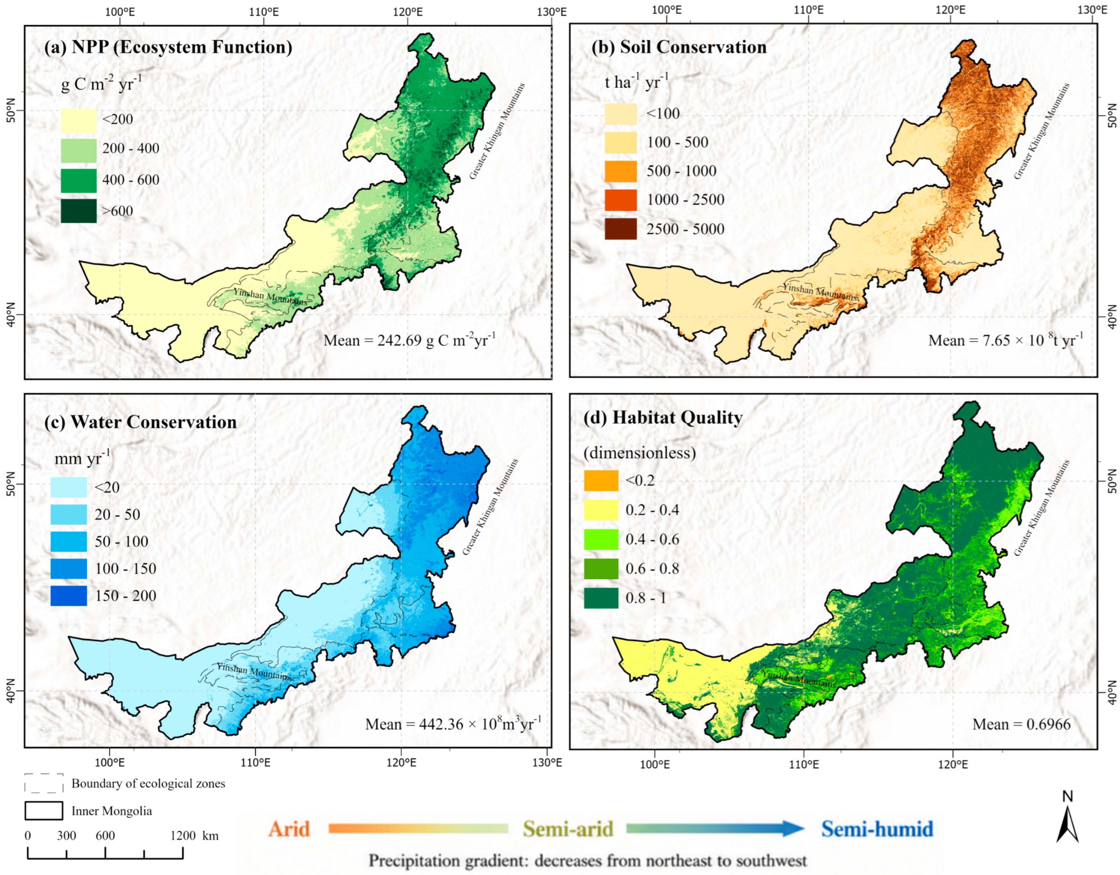
During 2001–2020, NPP formed a distinct northeast–southwest gradient across Inner Mongolia (Figure 2a). High values were concentrated in the Greater Khingan Mountains, Yanshan Mountains, and West Liaohe Plain, while the lowest values occurred in the western arid and desert regions. The regional mean NPP was 242.69 g C m−2 yr−1. Among ecological regions, mean NPP ranged from 43.37 g C m−2 yr−1 in the western Inner Mongolia Plateau and northwestern Ordos Plateau to 476.36 g C m−2 yr−1 in the Greater Khingan Mountains. The Yanshan Mountains and West Liaohe Plain also had relatively high mean values, at 389.92 and 282.64 g C m−2 yr−1, respectively. Most high-value areas exceeded 400 g C m−2 yr−1, whereas large parts of western Inner Mongolia were below 200 g C m−2 yr−1. Soil conservation showed a spatial pattern characterized by high values in mountainous areas and low values in plains, deserts, and western arid regions (Figure 2b). The multi-year mean annual soil conservation was 7.65 × 10⁸ t yr−1. Areas with soil conservation greater than 1000 t ha−1 yr−1 were mainly distributed in the Greater Khingan Mountains, Yanshan Mountains, and Yinshan Mountains. In contrast, most western and northwestern regions were dominated by values lower than 100 t ha−1 yr−1. Water conservation was also unevenly distributed across the region (Figure 2c). The multi-year mean annual water conservation was 442.36 × 10⁸ m3 yr−1. High-value areas were mainly located in the northeastern and southeastern parts of Inner Mongolia, especially in the Greater Khingan Mountains, West Liaohe Plain, and Yanshan Mountains. Low-value areas were mainly distributed in western Inner Mongolia, where most pixels were below 20 mm yr−1. Habitat quality presented a strong east–west contrast (Figure 2d). The regional mean habitat quality was 0.6966. Areas with habitat quality higher than 0.8 were mainly distributed in the Greater Khingan Mountains and eastern Inner Mongolia Plateau. Lower values were concentrated in the western arid region and in some areas with relatively intensive land use, where habitat quality was mostly below 0.4–0.6.
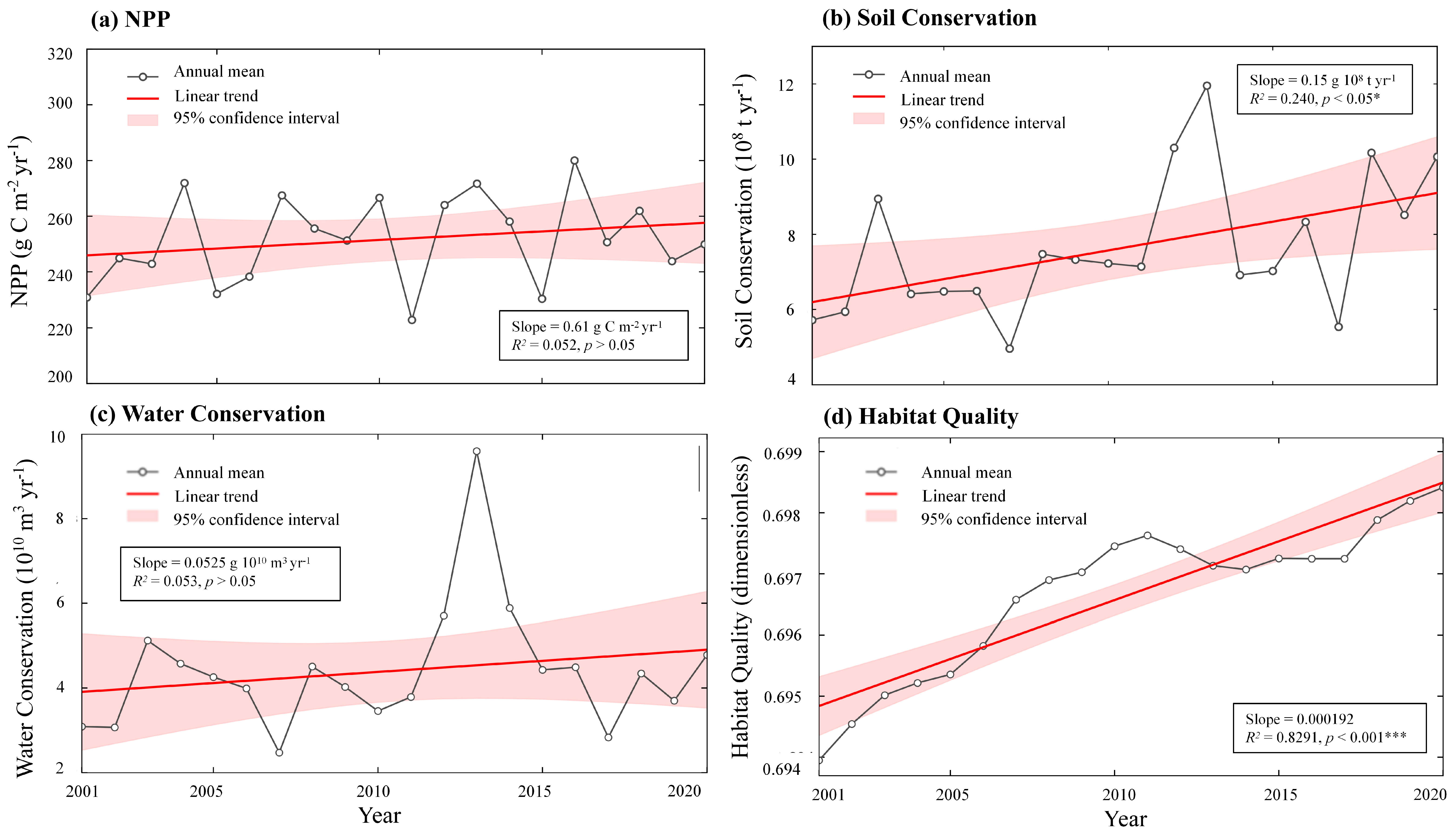
The annual trajectories of the four indicators showed different temporal patterns during 2001–2020 (Figure 3). NPP fluctuated substantially among years, with a weak positive linear trend. The fitted slope was 0.61 g C m−2 yr−1, and the trend was not statistically significant (R2 = 0.052, p > 0.05). Soil conservation showed a stronger upward trend, with a slope of 0.15 × 10⁸ t yr−1. This trend was statistically significant (R2 = 0.240, p < 0.05). Water conservation also increased over time, but with pronounced interannual variability. The fitted slope was 0.0525 × 10¹⁰ m3 yr−1, and the trend was not statistically significant (R2 = 0.053, p > 0.05). The annual series included a clear peak around 2013, followed by lower values in subsequent years. Habitat quality showed the most stable temporal trajectory among the four indicators. It increased steadily from 2001 to 2020, with a slope of 0.000192 and a significant linear trend (R2 = 0.8291, p < 0.001).
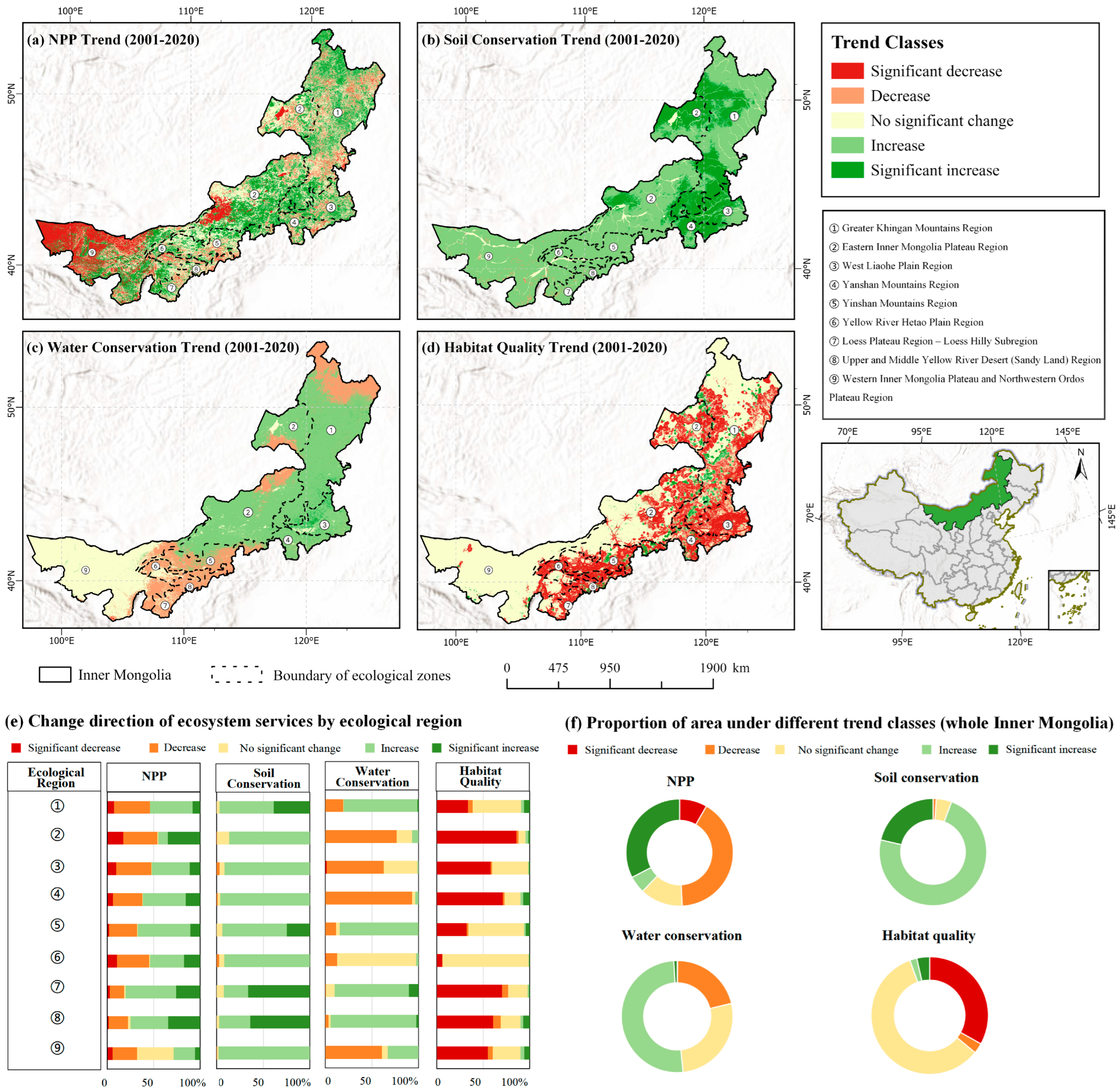
The trend classification further showed that the direction and significance of change differed among the four indicators (Figure 4). NPP contained both increasing and decreasing areas, with decreases mainly distributed in parts of western Inner Mongolia and transitional zones, and increases scattered across central and eastern regions. Soil conservation was dominated by increasing and significantly increasing trends, especially in mountainous and eastern regions. Water conservation showed a more fragmented pattern, with increasing trends mainly in eastern and central Inner Mongolia and decreasing trends in parts of the central–western arid and semi-arid regions. Habitat quality showed extensive areas of no significant change, together with localized significant decreases in the eastern and central parts of the region.
Across 2001–2020, the four indicators shared a broad spatial contrast between the forested and mountainous eastern regions and the arid western regions, but their temporal trajectories were not synchronous. Soil conservation showed the most evident increase, water conservation was characterized by large interannual fluctuations, NPP exhibited spatially mixed changes, and habitat quality varied within a relatively narrow range at the regional scale.

3.2. Comprehensive Ecological Benefit Index

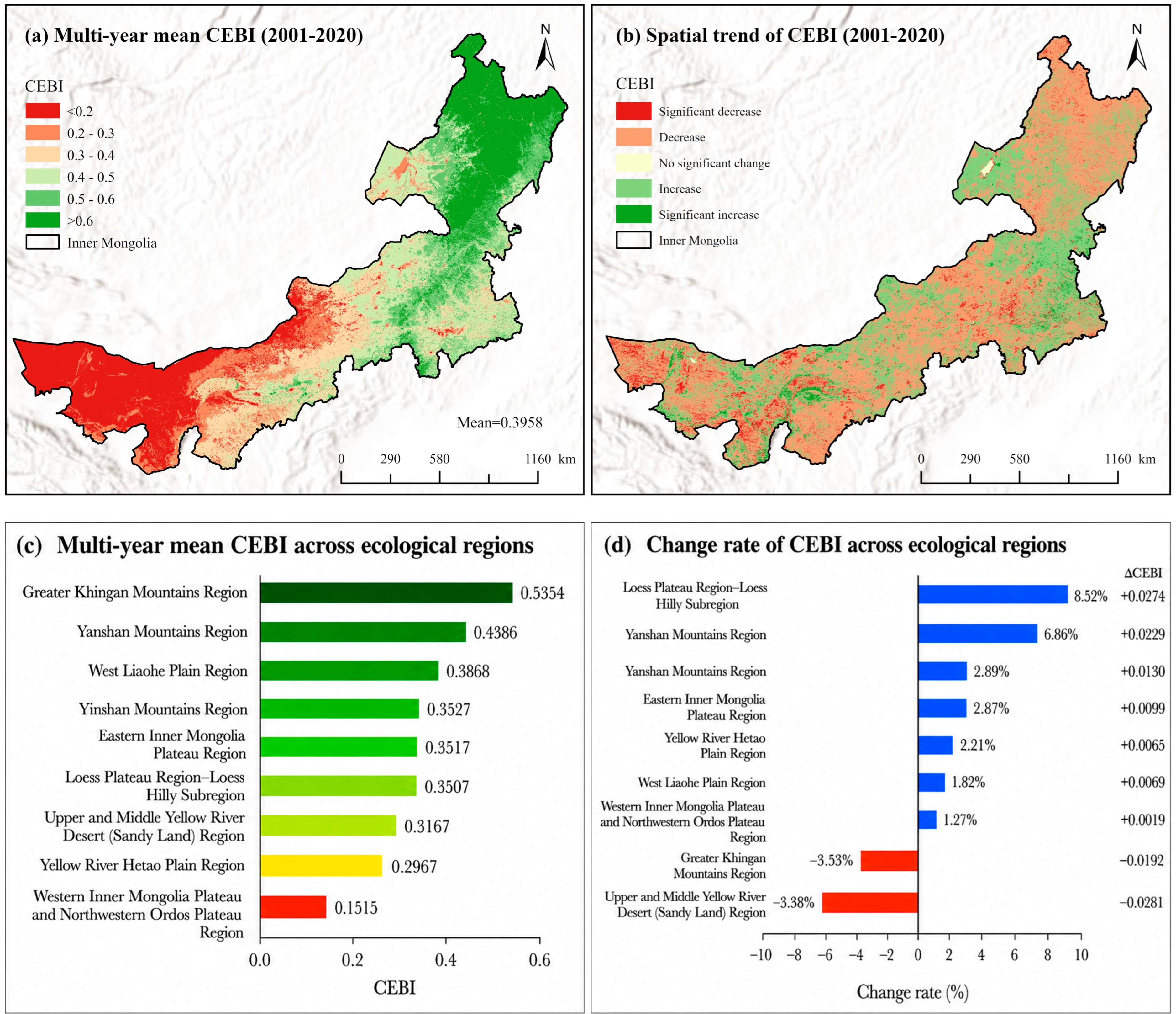
The comprehensive ecological benefit index (CEBI) displayed a pronounced spatial gradient across Inner Mongolia during 2001–2020 (Figure 5a). The multi-year mean CEBI for the whole region was 0.3958. Higher CEBI values were mainly concentrated in northeastern Inner Mongolia, especially in the Greater Khingan Mountains, whereas lower values were distributed predominantly in western Inner Mongolia. Moderate CEBI values extended across the central and southeastern parts of the region, including the Yanshan Mountains, West Liaohe Plain, Yinshan Mountains, and eastern Inner Mongolia Plateau. The spatial pattern of CEBI therefore highlighted a clear contrast between the northeastern mountainous region and the western arid region.
At the ecological-region scale, CEBI varied considerably among regions (Figure 5c). The Greater Khingan Mountains had the highest multi-year mean CEBI, with a value of 0.5354, followed by the Yanshan Mountains (0.4386) and the West Liaohe Plain (0.3868). The Yinshan Mountains, eastern Inner Mongolia Plateau, and Loess Plateau Region–Loess Hilly Subregion had comparable intermediate values, at 0.3527, 0.3517, and 0.3507, respectively. Lower values were recorded in the Upper and Middle Yellow River Desert Region (0.3167) and Yellow River Hetao Plain (0.2967). The lowest CEBI occurred in the western Inner Mongolia Plateau and northwestern Ordos Plateau, with a value of 0.1515.
The temporal trend of CEBI from 2001 to 2020 showed clear regional differences (Figure 5b,d). Increasing trends were mainly distributed in parts of the central mountainous areas and in scattered areas of eastern and southwestern Inner Mongolia, whereas decreasing trends occurred widely in western Inner Mongolia and some central–eastern transitional zones. At the ecological-region scale, the largest increase occurred in the Loess Plateau Region–Loess Hilly Subregion, with a relative change rate of 8.52% and an absolute increase of 0.0274. The Yinshan Mountains also increased by 6.86%, corresponding to an absolute increase of 0.0229. Smaller increases were observed in the Yanshan Mountains (2.89%, +0.0130), eastern Inner Mongolia Plateau (2.87%, +0.0099), Yellow River Hetao Plain (2.21%, +0.0065), West Liaohe Plain (1.82%, +0.0069), and western Inner Mongolia Plateau and northwestern Ordos Plateau (1.27%, +0.0019). In contrast, CEBI decreased in the Greater Khingan Mountains (−3.53%, −0.0192) and the Upper and Middle Yellow River Desert Region (−8.38%, −0.0281).

3.3. Spatial Explanatory Factors and Interaction Effects

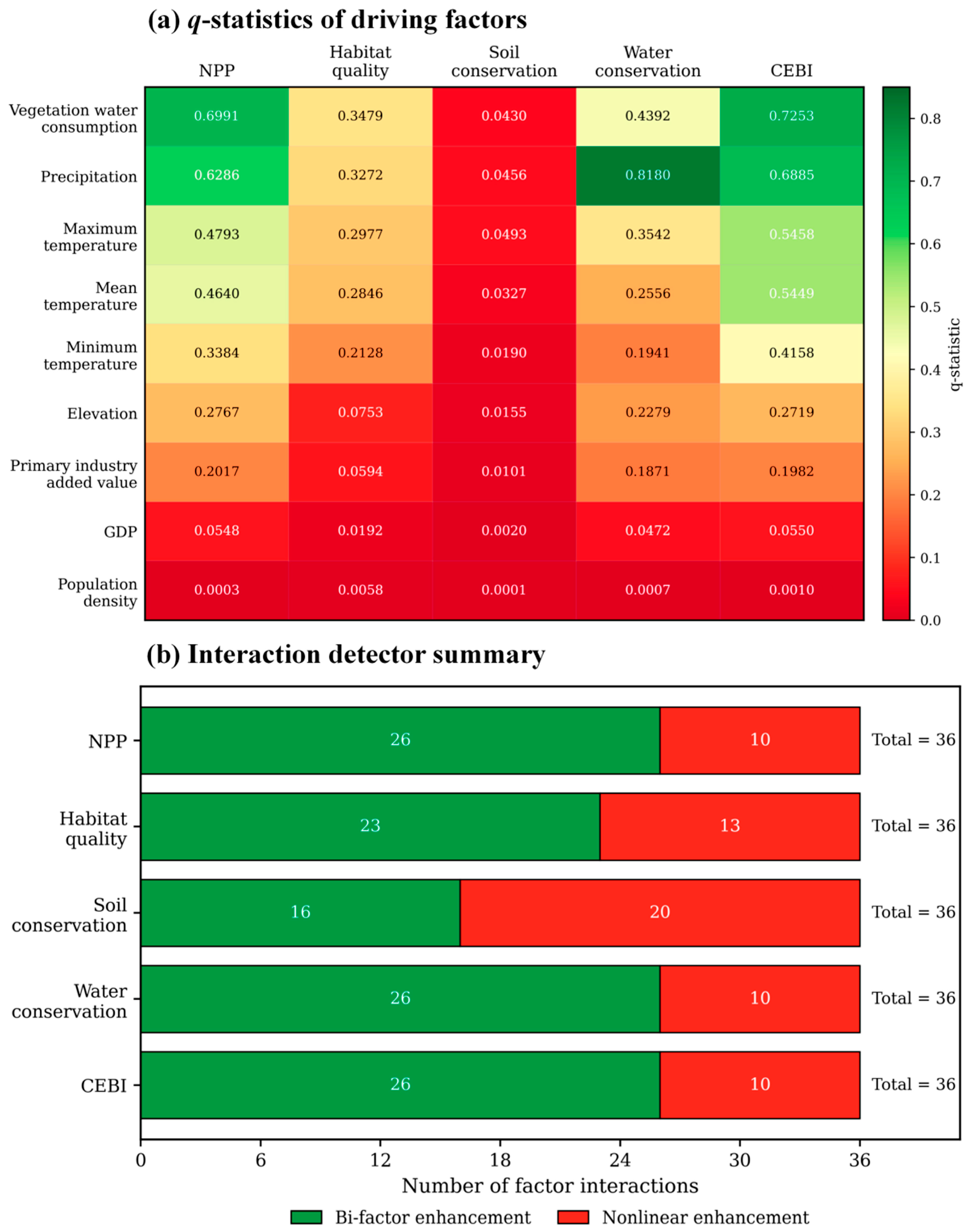
The factor detector showed distinct differences in conditional spatial explanatory power among indicators and candidate variables (Figure 6a). For NPP, vegetation water consumption had the highest q-statistic (0.6991), followed by precipitation (0.6286), maximum temperature (0.4793), mean temperature (0.4640), and minimum temperature (0.3384). A similar ranking occurred for CEBI: vegetation water consumption had q = 0.7253, followed by precipitation (0.6885), maximum temperature (0.5458), mean temperature (0.5449), and minimum temperature (0.4158). Socioeconomic variables had lower q-statistics at this regional scale; for example, GDP had q = 0.0548 for NPP and 0.0550 for CEBI, and population density was close to zero for all indicators. These values describe spatial concordance under the selected stratification and do not quantify causal effects.
The explanatory factors differed among ecosystem services. For water conservation, precipitation had the highest q-statistic among all factor–indicator combinations (0.8180), followed by vegetation water consumption (0.4392), maximum temperature (0.3542), mean temperature (0.2556), and elevation (0.2279). Habitat quality had lower q-statistics than NPP, water conservation, and CEBI. Vegetation water consumption ranked first for habitat quality (0.3479), followed by precipitation (0.3272), maximum temperature (0.2977), mean temperature (0.2846), and minimum temperature (0.2128). Soil conservation showed the weakest single-factor explanatory power. Its highest q-statistic was only 0.0493 for maximum temperature, followed by precipitation (0.0456), vegetation water consumption (0.0430), mean temperature (0.0327), and minimum temperature (0.0190).
The interaction detector results showed that paired variables enhanced explanatory power for all five indicators (Figure 6b). Among the 36 pairwise interactions for each indicator, no weakening or independent interaction was observed. NPP, water conservation, and CEBI each had 26 bi-factor enhancement interactions and 10 nonlinear enhancement interactions. Habitat quality had 23 bi-factor enhancement interactions and 13 nonlinear enhancement interactions. Soil conservation differed from the other indicators, with 16 bi-factor enhancement interactions and 20 nonlinear enhancement interactions. These results separate two spatial association patterns: vegetation water consumption and precipitation had relatively high single-variable q-values for NPP, water conservation, habitat quality, and CEBI, whereas soil conservation was characterized by low single-variable q-values and a higher proportion of nonlinear enhancement interactions.

4. Discussion

4.1. Spatial Heterogeneity and Asynchronous Changes in Ecosystem Functions and Services

The spatial distributions of NPP, water conservation, and habitat quality showed a consistent contrast between eastern and western Inner Mongolia. Higher values were concentrated in the Greater Khingan Mountains and adjacent eastern regions, whereas lower values occurred mainly in the western arid and semi-arid regions. This pattern is consistent with the strong east–west environmental gradient across Inner Mongolia, where relatively humid forested mountains gradually transition to grassland, desert, and plateau ecosystems [52,53,54]. In the eastern mountains, higher precipitation and denser vegetation cover provide favorable background conditions for vegetation productivity, hydrological regulation, and habitat maintenance [32,55]. In the western regions, limited water availability, sparse vegetation, and higher evaporative demand constrain the capacity of ecosystems to maintain multiple functions and services [56]. The broad spatial consistency among NPP, water conservation, and habitat quality therefore reflects the importance of hydroclimatic conditions and vegetation structure in shaping ecosystem service patterns across dryland transition zones.
Soil conservation differed from the other indicators in both spatial pattern and temporal change. Its high values were mainly concentrated in mountainous regions, including the Greater Khingan Mountains, Yanshan Mountains, and Yinshan Mountains, rather than following only the east–west vegetation gradient. This difference is related to the process represented by soil conservation. In the RUSLE-based assessment, soil conservation is calculated from the difference between potential and actual soil erosion; therefore, it depends not only on vegetation cover, but also on rainfall erosivity, slope, soil erodibility, and land-surface conditions [41,42]. Mountainous areas can have higher potential erosion because of steeper terrain, and vegetation cover in these areas can generate larger differences between potential and actual erosion [57,58,59]. Thus, high soil conservation values should be interpreted as strong erosion-retention capacity under specific terrain and surface conditions, rather than simply as high ecosystem quality.
The temporal trajectories of the four indicators were also not synchronous during 2001–2020. Soil conservation showed the most evident increase, whereas habitat quality changed within a narrow range. NPP showed weak change at the regional mean scale but differed among ecological regions, and water conservation fluctuated more strongly between years. These differences are consistent with the different ecological processes represented by each indicator. NPP responds to vegetation growth conditions and may vary among ecological zones even when the regional mean changes little [60,61]. Water conservation is closely linked to annual precipitation and evapotranspiration variability, which can produce stronger interannual fluctuations [62,63]. Habitat quality is largely determined by land-cover composition and the spatial distribution of threat sources, and therefore tends to change more gradually at the regional scale [42]. The asynchronous changes among indicators show that improvement in one ecosystem function or service does not necessarily correspond to simultaneous improvement in all others [64].

4.2. Comprehensive Ecological Benefits and Regional Differentiation

The CEBI results indicate that the four modelled ecological dimensions were characterized more by spatial differentiation than by a uniform temporal increase. Higher scores in forested and mountainous regions largely reflect greater absolute NPP, water conservation, and habitat-quality values under more humid conditions [16,65]. They should not be interpreted as evidence that forests are intrinsically more valuable or better functioning than arid grasslands and deserts. Dryland ecosystems provide distinctive services, may use scarce water more efficiently, and should be evaluated against ecosystem-specific baselines and constraints rather than a forest reference state. Accordingly, low CEBI in the western plateau denotes lower values for this particular four-indicator, absolute-capacity index, not lower ecological importance [66,67].
At the ecological-region scale, the CEBI pattern further separates ecological background conditions from temporal change. The Greater Khingan Mountains had the highest multi-year mean CEBI, followed by the Yanshan Mountains and West Liaohe Plain, whereas the western Inner Mongolia Plateau and northwestern Ordos Plateau had the lowest value. However, the temporal change rate did not follow the same ranking. The Loess Plateau Region–Loess Hilly Subregion and the Yinshan Mountains showed the largest increases in CEBI, while the Greater Khingan Mountains and the Upper and Middle Yellow River Desert Region showed declines. This contrast indicates that regions with high baseline ecological benefits did not necessarily experience continued improvement during 2001–2020. Conversely, some regions with intermediate baseline conditions showed more evident increases, suggesting that changes in integrated ecological benefits were regionally differentiated rather than simply controlled by the initial level of ecosystem service capacity [68].
The difference between individual indicators and CEBI is important for interpreting ecosystem change. Soil conservation increased most clearly, while CEBI still increased in some ecological regions and declined in others; improvement in one service may therefore coexist with stability or decline in another [65]. The linear additive score is useful for a consistent summary, but compensation is possible: a large increase in one component can offset a decrease in another, and ecological interactions, thresholds, and disservices are not represented. CEBI must therefore be read alongside the four component maps and trends. Its transfer to other regions would require reconsidering normalization bounds, the coefficient scheme, ecosystem-specific baselines, and the inclusion of biodiversity, wind-erosion control, water-use efficiency, cultural services, and other locally important dimensions [69].

4.3. Hydroclimatic and Vegetation-Related Spatial Associations

The Geographical Detector results show that spatial variation in the modelled indicators coincided more strongly with hydroclimatic and vegetation-related stratification than with the available socioeconomic variables. This pattern is consistent with Inner Mongolia’s water and energy gradients [38,70]. Precipitation determines the basic water input for vegetation growth and hydrological regulation, vegetation water consumption reflects vegetation-atmosphere water exchange, and temperature affects energy availability and evaporative demand. Thus, these variables remain ecologically meaningful background factors for spatial differences in productivity, hydrological regulation, habitat conditions, and integrated ecological benefits. However, precipitation is also an input to the water-balance calculation, vegetation water consumption overlaps with evapotranspiration-related processes, and water conservation contributes to CEBI. Therefore, high q-values involving these structurally related variable-response combinations should be interpreted as conditional spatial associations that may partly reflect model construction, rather than as evidence for ranking independent causal mechanisms.
The strongest spatial associations differed among indicators. NPP and CEBI had high q-values for vegetation water consumption and precipitation, while precipitation had the highest q-value for water conservation. For water conservation, this result is partly expected from the water-balance formulation and should be treated as an internal consistency pattern rather than independent attribution [71]. Habitat quality showed moderate q-values across several environmental variables, consistent with its dependence on land-cover composition, habitat suitability, threat intensity, and distance-decay assumptions [42]. The analysis therefore identifies where spatial stratifications coincide; it does not isolate direct and indirect causal pathways.
Soil conservation differed most clearly from the other indicators. Its single-factor q-statistics were all low, whereas the interaction detector identified a larger number of nonlinear enhancement interactions. This pattern does not imply that soil conservation lacked environmental controls. Rather, it reflects the compound nature of soil erosion and sediment retention. Soil conservation is shaped by the combined effects of rainfall erosivity, slope, soil erodibility, vegetation cover, and land-surface conditions [41,42]. A single factor may explain only a small fraction of its spatial heterogeneity, whereas paired factors can produce substantially stronger explanatory power. The higher proportion of nonlinear enhancement interactions for soil conservation is therefore consistent with the process complexity represented by the RUSLE-based sediment retention framework.
The weak single-factor q-statistics of GDP and population density should be interpreted with caution. At the regional scale, socioeconomic variables may not correspond directly to the spatial patterns of ecosystem functions and services, especially where broad hydroclimatic gradients dominate. In addition, human activities often affect ecosystem services indirectly through land-use change, ecological restoration, grazing intensity, infrastructure expansion, and management practices [72,73]. These pathways may not be fully represented by GDP or population density alone. The interaction results further showed that all paired factors enhanced explanatory power, indicating that ecosystem service variation in Inner Mongolia was associated with combined rather than isolated explanatory variables. This pattern supports the interpretation that hydroclimatic conditions, vegetation processes, terrain, and human-related factors jointly structure ecosystem service heterogeneity across the region.

4.4. Implications and Future Research

The spatial differentiation of ecosystem functions, services, and CEBI suggests that ecological management in Inner Mongolia should be adapted to regional ecological conditions. Forested and mountainous regions, particularly the Greater Khingan Mountains and Yanshan Mountains, maintained relatively high ecosystem service capacity and integrated ecological benefits. However, the decline in CEBI in the Greater Khingan Mountains indicates that high baseline ecological conditions do not necessarily correspond to continued improvement. For these regions, management should focus on maintaining ecosystem stability, reducing localized disturbance, and strengthening long-term monitoring of productivity, habitat quality, and water-related services. In contrast, the western Inner Mongolia Plateau and northwestern Ordos Plateau had persistently low CEBI values, suggesting that restoration strategies in arid and semi-arid regions should be designed within the limits of local water availability [73,74]. In such areas, matching vegetation type and restoration density with water conditions may be more appropriate than pursuing rapid increases in vegetation cover.
The asynchronous changes among individual indicators also have implications for restoration planning. Soil conservation showed the clearest increase, whereas water conservation fluctuated strongly and habitat quality changed only slightly at the regional scale. These differences indicate that single-objective restoration may not be sufficient for maintaining ecosystem multifunctionality [75]. Enhancement of erosion control, for example, does not necessarily imply simultaneous improvement in hydrological regulation or habitat conditions [76]. The strong interaction effects identified by the Geographical Detector further suggest that ecosystem service changes are associated with combined environmental and human-related factors. Future ecological management should therefore consider water availability, vegetation structure, terrain conditions, land-use change, and human disturbance together, rather than relying on single-factor interventions [77]. Regions with increasing CEBI, such as the Loess Plateau Region–Loess Hilly Subregion and the Yinshan Mountains, should be further monitored to determine whether these gains are stable and whether improvements in integrated ecological benefits are accompanied by balanced changes among individual services.
Several linked uncertainty sources should be considered. Input uncertainty arises from MODIS vegetation products, land-cover classification, precipitation, evapotranspiration, radiation correction, and spatial resampling. Parameter and structural uncertainty arises from CASA light-use efficiency, RUSLE and modified InVEST parameterization, habitat-threat distances and sensitivities, and the assumption that annual water balance represents water-conservation capacity [39,42,78]. Index uncertainty arises from min–max normalization and its temporal domain, the four-indicator selection, CEBI coefficient selection, and the linear compensatory structure of CEBI. Analytical uncertainty also arises from the discretization method and number of strata used by Geographical Detector.
These uncertainties may change absolute magnitudes and local rankings; consequently, management implications are framed at broad ecological-region scale rather than as pixel-level prescriptions.
Quantitative robustness tests using alternative CEBI coefficient schemes, InVEST parameter ranges, and Geographical Detector classifications are identified as priority analyses when the underlying raster and parameter datasets are available. Additional field observations and long-term monitoring would further constrain model uncertainty. CEBI also omits biodiversity, wind-erosion control, cultural services, and water-use efficiency [79,80].
The spatial explanatory-factor analysis has additional limitations. Geographical Detector identifies spatial concordance and interaction enhancement, not direct causal relationships [50,51]. Its q-statistics depend on spatial scale and discretization, and structural overlap is present where precipitation or vegetation water consumption contributes to a modelled response. Results are therefore described as conditional spatial associations. Future work should compare alternative driver sets that exclude embedded model inputs, test multiple discretization schemes, and combine process-based models, structural equation modelling, restoration boundaries, grazing intensity, land-use trajectories, and field experiments. Finer-resolution land use, climate extremes, and project-level information would help distinguish climate variability, restoration, and other human influences [81].

5. Conclusions

This study provides a 2001–2020, nine-region comparison of four modelled ecological dimensions and their integrated CEBI in Inner Mongolia. Change was spatially uneven and asynchronous: soil conservation increased most clearly, water conservation fluctuated strongly, NPP trends varied among regions, and land-cover-based habitat quality changed slowly. CEBI separated baseline capacity from temporal change—the Greater Khingan Mountains retained the highest mean score but declined, whereas the Loess Plateau–Loess Hilly Subregion and Yinshan Mountains increased most. Geographical Detector q-values identified conditional spatial associations with hydroclimatic and vegetation-related variables, not causal effects; structural overlap with model inputs further limits attribution. Management should therefore protect the stability of northeastern high-value ecosystems, match vegetation restoration and grazing pressure to water availability in western drylands, and evaluate erosion control together with hydrological and habitat outcomes. CEBI is a study-specific linear summary and must be interpreted with its component indicators, omitted services, model uncertainty, and discretization sensitivity. A full quantitative sensitivity analysis of alternative CEBI weighting schemes and key model parameterizations remains an important topic for future work.

Supplementary Materials

The following supporting information can be downloaded at: https://www.mdpi.com/article/10.3390/f17080968/s1.

Author Contributions

Conceptualization, C.C. and B.Q.; methodology, C.C. and J.W.; software, C.C. and L.W.; validation, C.C., Z.L. (Zhenyu Liu) and Z.L. (Ziye Liu); formal analysis, C.C.; investigation, J.W. and L.W.; resources, B.Q.; data curation, C.C. and Z.L. (Zhenyu Liu); writing—original draft preparation, C.C.; writing—review and editing, J.W., L.W., Z.L. (Zhenyu Liu), Z.L. (Ziye Liu) and B.Q.; visualization, C.C. and Z.L. (Ziye Liu); supervision, B.Q.; project administration, B.Q.; funding acquisition, B.Q. All authors have read and agreed to the published version of the manuscript.

Funding

This work was supported by the National Language Commission “14th Five-Year Plan” Scientific Research Planning 2023 Commissioned Project (WT145-37-4).

Data Availability Statement

The data that support the findings of this study are available from the corresponding author upon reasonable request. Publicly available input datasets are listed in Table 1 and Supplementary Table S1.

Conflicts of Interest

The authors declare no conflicts of interest.

References

  1. Costanza, R.; d’Arge, R.; de Groot, R.; Farber, S.; Grasso, M.; Hannon, B.; Limburg, K.; Naeem, S.; O’Neill, R.V.; Paruelo, J. The value of the world’s ecosystem services and natural capital. Nature 1997, 387, 253–260. [Google Scholar] [CrossRef] [Scilit]
  2. Ferraro, K.M.; Ferraro, A.L.; Lundgren, E.; Sommer, N.R. The use and abuse of ecosystem service concepts and terms. Biol. Conserv. 2025, 308, 111218. [Google Scholar] [CrossRef] [Scilit]
  3. Hernández-Blanco, M.; Costanza, R.; Chen, H.; de Groot, D.; Jarvis, D.; Kubiszewski, I.; Montoya, J.; Sangha, K.; Stoeckl, N.; Turner, K. Ecosystem health, ecosystem services, and the well-being of humans and the rest of nature. Glob. Change Biol. 2022, 28, 5027–5040. [Google Scholar] [CrossRef] [Scilit] [PubMed]
  4. Wang, M.; Wang, Y.; Liu, M.; Wang, Z.; Han, X.; Wu, Z. Assessment and Attribution of Ecosystem Services in Lvliang Mountains, a Semiarid–Semihumid Transitional Zone of China. Ecosyst. Health Sustain. 2026, 12, 0545. [Google Scholar] [CrossRef] [Scilit]
  5. Hao, Y.; Mao, J.; Bachmann, C.M.; Hoffman, F.M.; Koren, G.; Chen, H.; Tian, H.; Liu, J.; Tao, J.; Tang, J. Soil moisture controls over carbon sequestration and greenhouse gas emissions: A review. npj Clim. Atmos. Sci. 2025, 8, 16. [Google Scholar] [CrossRef] [Scilit]
  6. Huxman, T.E.; Smith, M.D.; Fay, P.A.; Knapp, A.K.; Shaw, M.R.; Loik, M.E.; Smith, S.D.; Tissue, D.T.; Zak, J.C.; Weltzin, J.F. Convergence across biomes to a common rain-use efficiency. Nature 2004, 429, 651–654. [Google Scholar] [CrossRef] [Scilit] [PubMed]
  7. Kaplan, A.; Khan, M.N.; Hayat, K.; Iqbal, M.; Ali, B.; Wahab, S.; Wahid, N.; Kanwal. Coupling Environmental Factors and Climate Change: Impacts on Plants and Vegetation Growth Patterns in Ecologically Sensitive Regions. In Environment, Climate, Plant and Vegetation Growth; Fahad, S., Saud, S., Nawaz, T., Gu, L., Ahmad, M., Zhou, R., Eds.; Springer: Cham, Switzerland, 2024; pp. 307–358. [Google Scholar] [CrossRef] [Scilit] [PubMed]
  8. Tariq, A.; Sardans, J.; Zeng, F.; Graciano, C.; Hughes, A.C.; Farré-Armengol, G.; Peñuelas, J. Impact of aridity rise and arid lands expansion on carbon-storing capacity, biodiversity loss, and ecosystem services. Glob. Change Biol. 2024, 30, e17292. [Google Scholar] [CrossRef] [Scilit] [PubMed]
  9. Hölting, L.; Beckmann, M.; Volk, M.; Cord, A.F. Multifunctionality assessments–More than assessing multiple ecosystem functions and services? A quantitative literature review. Ecol. Indic. 2019, 103, 226–235. [Google Scholar] [CrossRef] [Scilit]
  10. Yan, J.; Lou, B.; He, X. Forest ecosystem health assessment: Frameworks, challenges, and strategies for the future. Ecosyst. Health Sustain. 2025, 11, 0414. [Google Scholar] [CrossRef] [Scilit]
  11. Liu, X.; Li, H.; Zhou, Y.; Wang, X. Spatiotemporal dynamics of vegetation net primary productivity in Chinese ecological function conservation areas: The influences of climate and topography. J. Nat. Conserv. 2025, 84, 126846. [Google Scholar] [CrossRef] [Scilit]
  12. Zhou, J.; Chen, W.; Cai, Y.; Meng, Y.; Wang, Y.; Liu, Q.; Luo, S.; Peng, J. Effects of landscape pattern changes on ecosystem services: A case study of Ruoergai Plateau. Sci. Rep. 2025, 15, 45753. [Google Scholar] [CrossRef] [Scilit]
  13. Chen, L.; Wei, W. Time-lag and accumulation effects of climate change on habitat quality in the Chinese loess plateau. Ecosyst. Health Sustain. 2025, 11, 0360. [Google Scholar] [CrossRef] [Scilit]
  14. Dou, X.; Li, X.; Sang, G.; Yang, P.; Zhang, Y.; Wang, J.; Zhong, Z.; Lin, F.; Zhao, Q. Quantifying the impacts of climate change and human activities on vegetation in ecologically fragile regions: A case study of Northern China. Theor. Appl. Clim. 2025, 156, 259. [Google Scholar] [CrossRef] [Scilit]
  15. Yi, K.; Zhang, J.; Lei, H.; Chen, W.; Zhang, Y.; Fu, S.; Wang, K. Response of ecological condition in ecologically fragile areas to disturbance from extreme precipitation event: An empirical analysis from the loess plateau. J. Clean. Prod. 2025, 512, 145701. [Google Scholar] [CrossRef] [Scilit]
  16. Huang, F.; Zuo, L.; Gao, J.; Jiang, Y.; Du, F.; Zhang, Y. Exploring the driving factors of trade-offs and synergies among ecological functional zones based on ecosystem service bundles. Ecol. Indic. 2023, 146, 109827. [Google Scholar] [CrossRef] [Scilit]
  17. Ma, C.; Zhang, C.; Luo, Z.; Ji, L. Hydroclimatic Thresholds Shape the Long-Term Persistence of Net Ecosystem Productivity in the Yellow River Basin (2001–2024). Earth Syst. Environ. 2026, 1–20. [Google Scholar] [CrossRef] [Scilit]
  18. Zhang, S.; Tang, H.; Wang, Y.; Jin, Z.; Ci, M.; Liu, X.; Wang, H.; Ruan, J.; Niu, A.; Deng, J.; et al. Long-term trajectories of vegetation structure and function in China: Greening does not always indicate enhanced productivity. J. Clean. Prod. 2026, 568, 148725. [Google Scholar] [CrossRef] [Scilit]
  19. Wang, J.; Li, K.; Xu, S.; Shao, Y.; Wang, M.; Li, M.; Zhang, Y.; Liu, Y.; Li, F.; Altansukh, O.; et al. Issues, Progress, and Recommendations in the Construction of Ecological Barrier on the Mongolian Plateau from the Perspective of Big Data. J. Resour. Ecol. 2024, 15, 1113–1124. [Google Scholar] [CrossRef] [Scilit]
  20. Li, T.; Jia, Y.; Fava, F.; Xu, Z.; Zhu, J.; Yang, Y.; Tang, L.; Wang, Y.; Hao, Y.; Cui, X. A geographic identification of sustainable development obstacles and countermeasures in drylands: A case study in Inner Mongolia, China. Ecol. Indic. 2021, 132, 108257. [Google Scholar] [CrossRef] [Scilit]
  21. Williams, D.M. Beyond Great Walls: Environment, Identity, and Development on the Chinese Grasslands of Inner Mongolia; Stanford University Press: Redwood City, CA, USA, 2002. [Google Scholar]
  22. Hossain, M.L.; Lai, D.Y.F. Enhanced net primary productivity across Inner Mongolian grasslands despite diverging stability under climate perturbations. BMC Plant Biol. 2026, 26, 1351. [Google Scholar] [CrossRef] [Scilit] [PubMed]
  23. Mei, L.; Tong, S.; Yin, S.; Bao, Y.; Huang, X.; Alateng, T.; Wang, Y.; Guo, E.; Yuan, Z.; Nashun, D. Spatiotemporal variations of water use efficiency and its driving factors in Inner Mongolia from 2001 to 2020. J. Geogr. Sci. 2023, 33, 169–194. [Google Scholar] [CrossRef] [Scilit]
  24. Zhang, G.; Kang, Y.; Han, G.; Sakurai, K. Effect of climate change over the past half century on the distribution, extent and NPP of ecosystems of Inner Mongolia. Glob. Change Biol. 2011, 17, 377–389. [Google Scholar] [CrossRef] [Scilit]
  25. Duan, Q.; Liu, G. China: Ecological Restoration Projects for Connected Landscapes. In Ecological Connectivity of Forest Ecosystems; Lapin, K., Oettel, J., Braun, M., Konrad, H., Eds.; Springer: Cham, Switzerland, 2025; pp. 507–519. [Google Scholar] [CrossRef] [Scilit]
  26. Guan, X.; Wang, S.; Xu, M.; Ji, J.; Cao, C. Long-term ecological effectiveness of the Three-North Shelterbelt Program assessed by changes in ecosystem services. Sci. Rep. 2026, 16, 8330. [Google Scholar] [CrossRef] [Scilit] [PubMed]
  27. Zhai, J.; Wang, L.; Liu, Y.; Wang, C.; Mao, X. Assessing the effects of China’s three-north shelter forest program over 40 years. Sci. Total Environ. 2023, 857, 159354. [Google Scholar] [CrossRef] [Scilit] [PubMed]
  28. Fu, B.; Zhang, L.; Xu, Z.; Zhao, Y.; Wei, Y.; Skinner, D. Ecosystem services in changing land use. J. Soils Sediments 2015, 15, 833–843. [Google Scholar] [CrossRef] [Scilit]
  29. Zhang, H.; Peng, L.; Qiu, Y.; Ma, Z. What are the differences between ecosystem services and residents’ perceptions? Insights from perception gap, heterogeneity, and cross-level driving mechanisms. Appl. Geogr. 2026, 186, 103808. [Google Scholar] [CrossRef] [Scilit]
  30. Tong, S.; Zhang, J.; Ha, S.; Lai, Q.; Ma, Q. Dynamics of fractional vegetation coverage and its relationship with climate and human activities in Inner Mongolia, China. Remote Sens. 2016, 8, 776. [Google Scholar] [CrossRef] [Scilit]
  31. Wu, J.; Zhang, Q.; Li, A.; Liang, C. Historical landscape dynamics of Inner Mongolia: Patterns, drivers, and impacts. Landsc. Ecol. 2015, 30, 1579–1598. [Google Scholar] [CrossRef] [Scilit]
  32. Xia, Y.; Dan, D.; Liu, H.; Zhou, H.; Wan, Z. Spatiotemporal distribution of precipitation over the Mongolian Plateau during 1976–2017. Atmosphere 2022, 13, 2132. [Google Scholar] [CrossRef] [Scilit]
  33. Wang, W.; Guo, J. Regionalization and Analysis of Precipitation Variations in Inner Mongolia. Atmosphere 2025, 16, 216. [Google Scholar] [CrossRef] [Scilit]
  34. Guo, G.; Zou, X.; Zhang, Y. The Dual Effects of Climate Change and Human Activities on the Spatiotemporal Vegetation Dynamics in the Inner Mongolia Plateau from 1982 to 2022. Land 2025, 14, 1559. [Google Scholar] [CrossRef] [Scilit]
  35. Yan, X.; Wei, D.; Yang, J.; Yao, W.; Tian, S. Monitoring Temperate Typical Steppe Degradation in Inner Mongolia: Integrating Ecosystem Structure and Function. Sustainability 2025, 17, 9015. [Google Scholar] [CrossRef] [Scilit]
  36. Zhai, Y.; Wang, Y.; Hao, L.; Qi, W. Medium- and long-term independent contributions of climate change, management measures and land conversion to vegetation dynamics and inspiration for ecological restoration in Inner Mongolia, China. Ecol. Eng. 2025, 212, 107504. [Google Scholar] [CrossRef] [Scilit]
  37. Li, T.; Chen, P.; Lin, J.; Wu, Q.; Zhang, H.; Zhan, J. Quality Assessment and Identification of Key Areas for Ecological Conservation Projects in Inner Mongolia. Land 2025, 14, 438. [Google Scholar] [CrossRef] [Scilit]
  38. Li, S.; Qu, S.; Zhang, G.; Zhou, Y.; Sun, X.; Li, J.; Zhang, S. Spatiotemporal pattern and drivers of ecological quality in Inner Mongolia. Land 2024, 13, 568. [Google Scholar] [CrossRef] [Scilit]
  39. Potter, C.S.; Randerson, J.T.; Field, C.B.; Matson, P.A.; Vitousek, P.M.; Mooney, H.A.; Klooster, S.A. Terrestrial ecosystem production: A process model based on global satellite and surface data. Glob. Biogeochem. Cycles 1993, 7, 811–841. [Google Scholar] [CrossRef] [Scilit]
  40. Breiman, L.; Friedman, J.H.; Stone, C.J.; Olshen, R.A. Classification and Regression Trees; Chapman & Hall: New York, NY, USA, 1984. [Google Scholar]
  41. Renard, K.G.; Foster, G.R.; Weesies, G.A.; McCool, D.K.; Yoder, D.C. Predicting Soil Erosion by Water: A Guide to Conservation Planning with the Revised Universal Soil Loss Equation (RUSLE); Agriculture Handbook No. 703; U.S. Department of Agriculture: Washington, DC, USA, 1997.
  42. Natural Capital Project. InVEST 3.9.0 User Guide; Stanford University: Stanford, CA, USA, 2020; Available online: https://storage.googleapis.com/releases.naturalcapitalproject.org/invest/3.9.0/userguide/index.html (accessed on 23 July 2026).
  43. Sen, P.K. Estimates of the regression coefficient based on Kendall’s tau. J. Am. Stat. Assoc. 1968, 63, 1379–1389. [Google Scholar] [CrossRef] [Scilit]
  44. Kendall, M.G. Rank Correlation Methods, 4th ed.; Charles Griffin: London, UK, 1975. [Google Scholar]
  45. Mann, H.B. Nonparametric tests against trend. Econometrica 1945, 13, 245–259. [Google Scholar] [CrossRef] [Scilit]
  46. Zadeh, L.A. Fuzzy sets. Inf. Control 1965, 8, 338–353. [Google Scholar] [CrossRef] [Scilit]
  47. Comrey, A.L.; Lee, H.B. A First Course in Factor Analysis, 2nd ed.; Psychology Press: New York, NY, USA, 2013. [Google Scholar] [CrossRef] [Scilit]
  48. Bartlett, M.S. A note on the multiplying factors for various chi-square approximations. J. R. Stat. Soc. Ser. B 1954, 16, 296–298. [Google Scholar] [CrossRef] [Scilit]
  49. Kaiser, H.F. An index of factorial simplicity. Psychometrika 1974, 39, 31–36. [Google Scholar] [CrossRef] [Scilit]
  50. Wang, J.F.; Li, X.H.; Christakos, G.; Liao, Y.L.; Zhang, T.; Gu, X.; Zheng, X.Y. Geographical detector-based health risk assessment and its application in the neural tube defects study of the Heshun Region, China. Int. J. Geogr. Inf. Sci. 2010, 24, 107–127. [Google Scholar] [CrossRef] [Scilit]
  51. Geng, J.; Ji, H.; Hao, L. Quantitative assessment of climate change, land conversion, and management measures on key ecosystem services in arid and semi-arid regions: A case study of Inner Mongolia, China. Sustainability 2025, 17, 6348. [Google Scholar] [CrossRef] [Scilit]
  52. Li, H.; Guo, J.; Wang, Y.; Wang, W.; Jia, Q.; Wan, H.; Li, F.Y. Boundary migration between zonal vegetation types in Inner Mongolia over the past two decades. Catena 2024, 246, 108354. [Google Scholar] [CrossRef] [Scilit]
  53. Ma, W.; Zhao, C.; Zhou, N. Identifying the Factors Driving Vegetation Dynamics in Arid, Semiarid, and Semihumid Regions of the Mongolian Plateau. Ecosyst. Health Sustain. 2025, 11, 0407. [Google Scholar] [CrossRef] [Scilit]
  54. Feng, S.; Liu, X.; Zhao, W.; Yao, Y.; Zhou, A.; Liu, X.; Pereira, P. Key areas of ecological restoration in Inner Mongolia based on ecosystem vulnerability and ecosystem service. Remote Sens. 2022, 14, 2729. [Google Scholar] [CrossRef] [Scilit]
  55. Gao, B.; Ye, X.; Ding, L.; Zhang, P.; Wang, Y.; Xiao, L. Water availability dominated vegetation productivity of Inner Mongolia grasslands from 1982 to 2015. Ecol. Indic. 2023, 151, 110291. [Google Scholar] [CrossRef] [Scilit]
  56. Dai, Y.; Tian, L.; Zhu, P.; Dong, Z.; Zhang, R. Dynamic aeolian erosion evaluation and ecological service assessment in Inner Mongolia, northern China. Geoderma 2022, 406, 115518. [Google Scholar] [CrossRef] [Scilit]
  57. Tian, T.; Yang, Z.; Guo, J.; Zhang, T.; Wang, Z.; Miao, P. Spatiotemporal evolution of soil erosion and its driving mechanism in the Mongolian section of the Yellow River Basin. Land 2023, 12, 801. [Google Scholar] [CrossRef] [Scilit]
  58. Tuvshinjargal, N.; Lamchin, M.; Kim, Y.; Bayarmagnai, E.; Jeon, S.W. Assessment of potential soil erosion in Mongolia based on the RUSLE model and RCP 8.5 scenario. Soil Use Manag. 2024, 40, e13005. [Google Scholar] [CrossRef] [Scilit]
  59. Ma, B.; Jing, J.; Liu, B.; Wang, Y.; He, H. Assessing the contribution of human activities and climate change to the dynamics of NPP in ecologically fragile regions. Glob. Ecol. Conserv. 2023, 42, e02393. [Google Scholar] [CrossRef] [Scilit]
  60. Wei, X.; Yang, J.; Luo, P.; Lin, L.; Lin, K.; Guan, J. Assessment of the variation and influencing factors of vegetation NPP and carbon sink capacity under different natural conditions. Ecol. Indic. 2022, 138, 108834. [Google Scholar] [CrossRef] [Scilit]
  61. Workneh, M.; Mekoya, A.; Tesema, H.A. Recent Trends and Variability in Climatic Water Balance: Implications for Forestry Development in Ethiopia. Meteorol. Appl. 2025, 32, e70124. [Google Scholar] [CrossRef] [Scilit]
  62. Zhang, Q.; Bao, Y. Spatiotemporal Variation Patterns of and Response Differences in Water Conservation in China’s Nine Major River Basins Under Climate Change. Atmosphere 2025, 16, 837. [Google Scholar] [CrossRef] [Scilit]
  63. Hu, Z.; Dakos, V.; Rietkerk, M. Using functional indicators to detect state changes in terrestrial ecosystems. Trends Ecol. Evol. 2022, 37, 1036–1045. [Google Scholar] [CrossRef] [Scilit] [PubMed]
  64. Liu, J.; Pei, X.; Zhu, W.; Jiao, J. Water-related ecosystem services interactions and their natural-human activity drivers: Implications for ecological protection and restoration. J. Environ. Manag. 2024, 352, 120101. [Google Scholar] [CrossRef] [Scilit] [PubMed]
  65. Dai, Z.-Z.; Zou, L.; Xie, X.-Y.; Duan, J.-J.; Shi, X.-L.; Zhu, Z.-Y.; Feng, Y.-Z.; Wang, X. Unlocking ecosystem service potential: Identifying high-sensitivity and high-potential ecological improvement areas in Inner Mongolia. J. Clean. Prod. 2025, 532, 146952. [Google Scholar] [CrossRef] [Scilit]
  66. Wu, L.; Fan, F. Assessment of ecosystem services in new perspective: A comprehensive ecosystem service index (CESI) as a proxy to integrate multiple ecosystem services. Ecol. Indic. 2022, 138, 108800. [Google Scholar] [CrossRef] [Scilit]
  67. Liang, X.; Yu, S.; Ju, Y.; Wang, Y.; Lü, H.; Li, L. Land-Use Change and Ecosystem Service Trade-Offs: What Multi-Scale Evidence Can and Cannot Tell Us for Sustainability Governance. Sustainability 2026, 18, 5833. [Google Scholar] [CrossRef] [Scilit]
  68. Taelman, S.E.; Schaubroeck, T.; De Meester, S.; Boone, L.; Dewulf, J. Accounting for land use in life cycle assessment: The value of NPP as a proxy indicator to assess land use impacts on ecosystems. Sci. Total Environ. 2016, 550, 143–156. [Google Scholar] [CrossRef] [Scilit] [PubMed]
  69. Mei, L.; Tong, S.; Yin, S.; Bao, Y.; Huang, X.; Alateng, T. Variation characteristics of ecosystem water use efficiency and its response to human activity and climate change in Inner Mongolia. Remote Sens. 2022, 14, 5422. [Google Scholar] [CrossRef] [Scilit]
  70. Zhang, P.; Liu, X.; Zhu, W.; Li, C.; Jin, R.; Yan, H.; Gu, C.; Wang, J. Spatio-temporal changes in water conservation ecosystem service during 1990–2019 in the Tumen River Basin, Northeast China. Chin. Geogr. Sci. 2023, 33, 102–115. [Google Scholar] [CrossRef] [Scilit]
  71. Fang, Y.; Meng, F.; Luo, M.; Sa, C.; Bao, Y.; Lei, J. Coupling coordination framework for assessing balanced development between potential ecosystem services and human activities. Earth’s Future 2025, 13, e2025EF006243. [Google Scholar] [CrossRef] [Scilit]
  72. Mir, Y.H.; Mir, S.; Ganie, M.A.; Bhat, J.A.; Shah, A.M.; Mushtaq, M.; Irshad, I. Overview of land use and land cover change and its impacts on natural resources. In Ecologically Mediated Development: Promoting Biodiversity Conservation and Food Security; Springer: Berlin/Heidelberg, Germany, 2025; pp. 101–130. [Google Scholar]
  73. Luo, Y.; Wu, L.; Wang, R.; Wang, X.; Du, B.; Pang, S. Will vegetation restoration affect the supply-demand relationship of water yield in an arid and semi-arid watershed? Sci. Total Environ. 2025, 959, 178292. [Google Scholar] [CrossRef] [Scilit] [PubMed]
  74. Li, Y.; Qi, S.; Li, J. Research on Ecological Restoration Technology in Arid or Semi-Arid Areas from the Perspective of the Belt and Road Initiative. J. Resour. Ecol. 2022, 13, 964–976. [Google Scholar] [CrossRef] [Scilit]
  75. He, J.; Li, Y.; Zhou, W.; Qian, M.; Zha, E.; Shi, X. A Multi-Objective Framework for Regional Ecological Planning: Restoration Prioritization Analysis. Land Degrad. Dev. 2025, 36, 3670–3684. [Google Scholar] [CrossRef] [Scilit]
  76. Li, H.; Yang, X.; Yu, Y.; Zhang, F.; Liu, Y.; Zhang, S. Optimizing soil and water conservation at the sub-basin scale: A multi-objective approach balancing ecosystem services, costs, and erosion control. Int. Soil Water Conserv. Res. 2026, 14, 100632. [Google Scholar] [CrossRef] [Scilit]
  77. Zhang, X.; Song, W. From static to predictive indicators: Construction of China’s spatiotemporal risk zoning index for land use changes ecological risks. Ecol. Indic. 2025, 179, 114154. [Google Scholar] [CrossRef] [Scilit]
  78. Wang, R.-Y.; Mo, X.; Ji, H.; Zhu, Z.; Wang, Y.-S.; Bao, Z.; Li, T. Comparison of the CASA and InVEST models’ effects for estimating spatiotemporal differences in carbon storage of green spaces in megacities. Sci. Rep. 2024, 14, 5456. [Google Scholar] [CrossRef] [Scilit] [PubMed]
  79. Jay, M.; Plieninger, T. Addressing landscape multifunctionality in conservation and restoration. Nat. Rev. Biodivers. 2025, 1, 717–732. [Google Scholar] [CrossRef] [Scilit]
  80. Ma, L.; Hong, L.; Liang, X. Integrating Ecological and Economic Approaches for Ecosystem Services and Biodiversity Conservation: Challenges and Opportunities. Ecologies 2025, 6, 70. [Google Scholar] [CrossRef] [Scilit]
  81. Suarez, D.C. Biologists Unite: The Rise and Fall of Ecosystem Services; The MIT Press: Cambridge, MA, USA, 2026. [Google Scholar] [CrossRef] [Scilit]
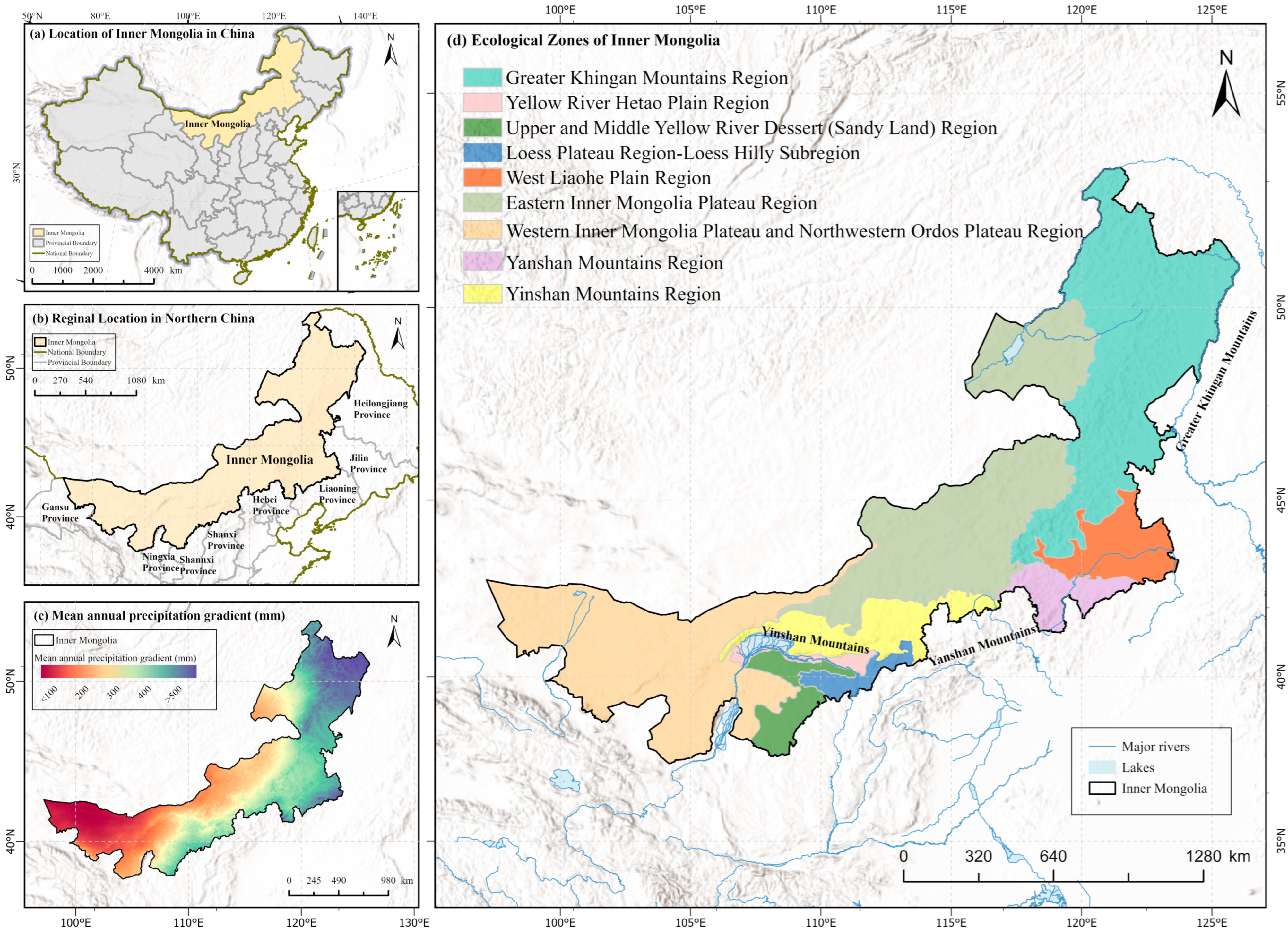
Figure 1. Location, environmental setting, and ecological regions of Inner Mongolia.
Forests 17 00968 g001
Figure 2. Spatial distributions of multi-year mean NPP, soil conservation, water conservation, and habitat quality in Inner Mongolia during 2001–2020.
Forests 17 00968 g002
Figure 3. Interannual variations in NPP, soil conservation, water conservation, and habitat quality in Inner Mongolia from 2001 to 2020. The red lines represent linear trends, and shaded areas indicate 95% confidence intervals. * indicates p < 0.05 and *** indicates p < 0.001.
Forests 17 00968 g003
Figure 4. Spatial trends and trend-class proportions of NPP, soil conservation, water conservation, and habitat quality during 2001–2020. Trend classes were identified based on Sen’s slope and the Mann–Kendall significance test.
Forests 17 00968 g004
Figure 5. Spatial patterns, temporal trends, and regional differences in the comprehensive ecological benefit index (CEBI) in Inner Mongolia during 2001–2020. (a) Spatial distribution of multi-year mean CEBI; (b) spatial trend of CEBI based on Sen’s slope and the Mann–Kendall test; (c) multi-year mean CEBI across ecological regions; and (d) relative change rate of CEBI across ecological regions from 2001 to 2020.
Forests 17 00968 g005
Figure 6. Spatial explanatory variables and interaction effects for ecosystem functions and services in Inner Mongolia. (a) q-statistics of individual variables for NPP, habitat quality, soil conservation, water conservation, and CEBI. Colors show conditional spatial explanatory power under the selected stratification; q-values do not establish causality. (b) Interaction detector summary showing the number of bi-factor and nonlinear enhancement interactions.
Forests 17 00968 g006
Table 1. Datasets used for ecosystem function and service assessment and spatial explanatory-factor analysis.
Data CategoryDataset/VariablesPeriodSourceMain Application
Vegetation remote sensingMODIS NDVI (MOD13A2 v061)2001–2020NASA MODISVegetation dynamics and NPP estimation
Meteorological dataMonthly precipitation; monthly mean, minimum, and maximum temperature; shortwave radiation2001–2020National Earth System Science Data Center; NASACASA model, water conservation assessment, and climatic explanatory-factor analysis
Land-cover and vegetation dataLand-cover type and vegetation type2001–2020ESA CCI Land CoverHabitat quality assessment, vegetation parameter assignment, and land-cover characterization
Hydrological and vegetation structure dataPotential evapotranspiration and leaf area index (LAI)2001–2020National Tibetan Plateau Data Center; Global Land Surface Satellite (GLASS)Water conservation assessment and vegetation-related parameter estimation
Road network dataTraffic road network2001–2020OpenStreetMapThreat-source data for habitat quality assessment
Ecological observationsGround solar radiation observations2017–2019Inner Mongolia forestry ecological stationsCART calibration and validation
Vegetation water-use and socioeconomic dataVegetation evapotranspiration (used as a proxy for vegetation water consumption), population density, GDP, and primary-industry added value2001–2020National Tibetan Plateau Data Center; WorldPop; Inner Mongolia Statistical YearbookSpatial explanatory-factor analysis using the Geographical Detector model
Disclaimer/Publisher’s Note: The statements, opinions and data contained in all publications are solely those of the individual author(s) and contributor(s) and not of MDPI and/or the editor(s). MDPI and/or the editor(s) disclaim responsibility for any injury to people or property resulting from any ideas, methods, instructions or products referred to in the content.