The Effects of Fiscal Policy on Forest Cover Conditions and Dynamics: Evidence from Tanzania

Abstract

Forest cover conditions in Tanzania remain predominantly negative, with significant implications for biodiversity, rural livelihoods, and climate stability. Despite national forest management policies, traceability systems, afforestation programs, REDD+ initiatives, and the National Carbon Monitoring Centre, forest conditions continue to deteriorate. Naturally regenerating forests declined to 42.8 million hectares in 2025, while annual deforestation rose to approximately 469 thousand hectares in the post-2015 period. Fire disturbances remain evident, with around 4014 hectares burned in 2025, and forest growing stock declined to 3143 million m³. Existing studies largely attribute these trends to agricultural expansion, population pressure, and charcoal dependence, while the role of fiscal policy has received limited empirical attention. This study addresses this gap by examining the relationship between fiscal policy and forest cover conditions in Tanzania from 2001 to 2024 using a VAR framework. The results indicate that increases in government development expenditure are associated with short-run improvements in forest cover conditions, suggesting that public investment can contribute to positive environmental outcomes, while balanced budget condition is associated with more stable improvements. These findings point to strengthened domestic revenue systems, greater fiscal discipline, and closer alignment of public expenditure with environmental objectives as relevant areas for further policy attention.

1. Introduction

Forests are among the most critical natural resources globally, covering approximately 30.8% of the terrestrial surface, equivalent to about 4.06 billion hectares [1]. However, their distribution is highly uneven, with more than half of global forest cover concentrated in a few countries. Forest ecosystems play a fundamental role in sustaining biodiversity, hosting nearly 80% of amphibian species, 75% of bird species, and 68% of mammal species, as well as over 60,000 tree species worldwide [2,3,4]. Beyond their ecological importance, forests are essential for human well-being, providing food, fuel, medicine, and income, while supporting approximately 86 million green jobs and the livelihoods of nearly 880 million people worldwide [1]. Forests are essential for food systems, climate regulation, and human health. They support pollination for about 75% of crops, provide wild foods for nearly one billion people, and supply cooking fuel for around 2.4 billion people [1]. Globally, forest cover dynamics indicate a persistent decline in naturally regenerating forests, which decreased from approximately 4132.6 million hectares in 1990 to 3808.2 million hectares in 2025 [5]. Although planted forests increased from about 183.6 million hectares to 303.6 million hectares over the same period, this increase has not fully offset the continued reduction in naturally regenerating forest ecosystems [5]. These trends reflect ongoing pressures on global forest systems and highlight persistent challenges for biodiversity conservation, carbon storage, and ecosystem sustainability. While global forest growing stock and carbon stock in biomass have slightly increased over time, these aggregate trends mask important regional disparities.

In Africa, forest cover dynamics remain predominantly negative, with naturally regenerating forests declining from approximately 770.6 million hectares in 1990 to 648.5 million hectares in 2025 [5]. Although planted forests increased from about 8.9 million hectares to 14.1 million hectares over the same period, the increase remains relatively small compared to the decline in naturally regenerating forests [5]. Similarly, forest growing stock declined from 99.22 billion m³ in 1990 to 85.13 billion m³ in 2025, alongside a reduction in biomass carbon stock from 65.45 Gt to 56.64 Gt over the same period [5]. These trends reflect continued pressures on forest ecosystems, largely associated with deforestation and land-use change [6].

Tanzania possesses substantial forest resources, with forest cover of approximately 48.1 million hectares, with woodlands alone covering about 50.6% of its land area [7]. These forests are central to the country’s economy and energy systems, contributing about 3.3% to GDP and supplying nearly half of national energy needs through biomass fuels [8]. However, forest cover dynamics in Tanzania have become increasingly negative over time. Naturally regenerating forests declined from about 57.6 million hectares in 1990 to 42.8 million hectares in 2025, while annual deforestation increased from about 403 thousand hectares during 1990–2015 to approximately 469 thousand hectares in the period after 2015 [5]. Forest ecosystems have also been affected by fire disturbances, with burned areas ranging from about 6643 hectares (2002) to a peak of approximately 10,524 hectares (2005), before declining to around 4014 hectares (2022), indicating persistent but fluctuating fire pressure [5]. In addition, forest growing stock declined from 4215 million m³ in 1990 to 3143 million m³ in 2025, indicating continued deterioration in forest conditions despite the existence of national and sub-national sustainable forest management policies and regulations [5]. These trends suggest persistent pressure on forest ecosystems driven mainly by agricultural expansion, charcoal production, population growth, and timber harvesting [9,10,11]. The resulting decline poses serious environmental and socio-economic risks, including biodiversity loss, disruption of ecosystem services, and increased greenhouse gas emissions.

Although existing studies have extensively examined the environmental and socio-economic drivers of forest cover dynamics and forest loss in Tanzania, limited attention has been given to the role of fiscal policy instruments in influencing forest cover conditions and dynamics. This represents a critical gap, given the potential of government fiscal mechanisms such as taxation, public expenditure, and budget allocation to influence environmental outcomes and sustainable forest management.

Therefore, this study analyzes the effects of fiscal policy on forest cover conditions and dynamics in Tanzania by examining how government expenditure, revenue, and budgetary decisions influence changes in forest conditions over time. By providing empirical evidence on this relationship, this study seeks to inform more effective and sustainable policy interventions that balance environmental conservation with socio-economic needs.

The remainder of this paper is organized as follows: Section 2 reviews the relevant literature on fiscal policy and forest cover dynamics. Section 3 describes the study area, theoretical framework, data, and econometric approach. Section 4 presents the empirical results, including model specification and diagnostic tests, regression estimates, and impulse response and variance decomposition analysis, followed by a discussion of the findings. Section 5 concludes with a summary of the results, policy implications, study limitations, and directions for future research.

2. Literature Review

The literature on forest cover conditions and dynamics in Tanzania consistently identifies agriculture as the dominant driver of deforestation [10,11,12,13,14]. However, there is ongoing debate on the relative importance of other drivers, particularly charcoal production and shifting cultivation. For example, agriculture is estimated to contribute between 110,000 and 150,000 hectares of deforestation annually (2011–2015), while charcoal production alone accounts for about 33.16% of deforestation, one of the highest rates globally [15,16]. In addition, studies highlight spatial variation in forest regeneration, with shifting cultivation acting as a regeneration driver in some areas but declining in others, reflecting strong regional heterogeneity [17,18]. Broader evidence further shows that both direct drivers (agriculture, logging, grazing, charcoal production) and indirect drivers (population growth, weak enforcement, and limited alternatives) jointly sustain forest loss, despite initiatives such as REDD+ [19].

In terms of forest conditions, studies in Tanzania show that biomass and carbon stocks vary significantly with management and disturbance levels. In miombo wood-lands, aboveground biomass ranges from about 37.9 tonnes per hectare in degraded forests to over 48 tonnes per hectare under participatory forest management, indicating improved forest conditions under stronger governance [20]. Similarly, dry miombo ecosystems store about 68.64 megagrams of carbon per hectare, reflecting higher carbon stocks in intact forests [21]. Forest land also contains substantially higher carbon than non-forest land uses, reinforcing the link between forest cover conditions and carbon stocks [22]. However, deforestation and degradation reduce biomass and carbon stocks by lowering forest density and structural integrity, while stable forest cover supports higher carbon retention and ecosystem resilience [23]. Overall, the literature indicates that forest cover dynamics strongly determine biomass and carbon variation in Tanzania, highlighting the need for stable and effective forest management to ensure long-term environmental sustainability.

Remote sensing studies such as [24] confirm substantial negative forest cover dynamics in the Eastern Arc Mountains but reveal limited regeneration. Overall, although there is consensus on agriculture as a key driver, the relative contribution of other factors remains contested, highlighting the need for integrated approaches combining socio-economic and geospatial analysis to better understand forest cover dynamics.

Early studies examined the macroeconomic effects of fiscal instruments such as environmental taxes, subsidies, and green public investment and found that these tools can promote sustainable growth by internalizing environmental externalities and reducing pollution levels [25]. Subsequent research extended this analysis using general equilibrium frameworks, demonstrating that the environmental and economic impacts of fiscal policies depend on their interaction with existing tax systems and market distortions, which can either enhance or offset their intended effects [26]. More recent contributions employ dynamic stochastic general equilibrium and computable general equilibrium models, showing that well-designed fiscal strategies can simultaneously support economic growth and reduce environmental degradation, particularly when policies are coordinated and efficiently implemented [27]. Despite broad agreement that fiscal policies can contribute to environmental sustainability, their effectiveness remains highly context-dependent. Empirical evidence suggests that outcomes vary with market conditions, policy design, and institutional capacity, with developing economies often facing additional constraints such as weak governance, limited enforcement, and structural inefficiencies.

The Environmental Kuznets Curve hypothesis further suggests an inverted U-shaped relationship between income and environmental degradation, including deforestation, although its validity remains debated [28,29]. Empirical applications using macroeconomic data show mixed results; ref. [30] highlights the importance of crop prices and trade openness in influencing deforestation through demand land conversion, while ref. [31] identifies U-shaped association between income and forest environmental degradation but acknowledges limitations in isolating fiscal policy impacts.

More recent empirical work directly links fiscal policy to environmental outcomes using VAR-based approaches [32]. It was found that balanced financed government expenditure can reduce pollution, while tax cuts may increase emissions, highlighting the asymmetric environmental effects of fiscal instruments. Similarly, ref. [33], using Brazilian data, shows that government expenditure can reduce deforestation, with both deficit and balanced budget fiscal shocks having mitigating effects, particularly when directed toward public goods. However, these findings are subject to limitations related to institutional differences that may affect external validity.

Much of the literature relies on aggregate fiscal data due to limited availability of disaggregated sectoral expenditure data, which constrains analysis of sector-specific environmental effects. This is particularly important in developing countries, where fiscal policy affects environmental outcomes through channels such as energy use, land-use decisions, and household production systems, making impacts highly context-dependent. In Tanzania, this transmission channel is especially relevant because environmental outcomes are closely linked to household energy choices. Biomass accounts for over 90% of total energy use, with most households relying on firewood (63.5%) and charcoal (26.2%), while only about 4.5% use clean cooking energy [34]. Fiscal policy influences these patterns through energy pricing and incentives; however, high costs and energy stacking limit the transition to cleaner fuels, resulting in continued reliance on charcoal and sustained pressure on forest resources.

Despite growing literature on macroeconomic–environmental linkages, there remains a clear gap in the Tanzanian context. Most existing studies focus on traditional drivers such as agriculture, charcoal production, and population pressure, while fiscal policy remains largely underexplored. Although international evidence suggests that government expenditure and taxation can influence environmental outcomes, these studies are concentrated in developed economies or large emerging economies such as Brazil and the United States.

This study addresses these gaps by focusing on Tanzania and employing a VAR framework to analyze the effects of fiscal policy instruments on forest cover conditions over time. In doing so, it contributes to existing VAR-based environmental studies by providing country-specific evidence on how taxation, public expenditure, and fiscal balance mechanisms influence forest cover conditions and dynamics in a Sub-Saharan African context. The findings are expected to inform policy design aimed at aligning fiscal policy with sustainable forest management and long-term environmental sustainability.

3. Materials and Methods

3.1. Study Area and Spatial Representation

The study area encompasses Tanzania, whose national boundaries define the spatial extent of the analysis and from which all geospatial datasets were derived. Forest cover data were obtained from the Hansen Global Forest Change dataset and processed within Google Earth Engine (Google LLC, Mountain View, CA, USA). A tree cover threshold of 30% for the year 2000 was applied to delineate the baseline forest extent.

For visualization purposes, three primary spatial layers were generated, baseline forest cover for 2000, remaining forest cover for 2024, and a forest dynamic map distinguishing no-forest areas, positive forest dynamics, and negative forest dynamics. All outputs were produced at a spatial resolution of 30 m and subsequently exported for further processing and cartographic visualization in QGIS (version 4.0.0; QGIS.org). For cartographic representation, a consistent classification and symbology scheme was applied, with positive forest dynamics depicted using a green color gradient, negative forest dynamics indicated in red, and no-forest areas represented in neutral tones, as illustrated in Figure 1. This map provides a spatial overview of forest distribution and dynamics across Tanzania and forms the basis for subsequent analyses of changes in forest conditions over time.

3.2. Theoretical Background

This study adopts the theoretical framework developed by [33], which models environmental outcomes as a function of the trade-off between economic activity and forest cover. The original model conceptualizes forest dynamics as being influenced by consumption, capital accumulation, and government fiscal interventions, where fiscal policy affects forest outcomes through its impact on consumption behavior and environmental degradation rates. Readers are referred to [33] for the full structural derivation of the model.

In simplified terms, the model establishes a direct link between fiscal policy and forest cover by showing that government expenditure and taxation influence resource consumption and the rate of environmental degradation, which, in turn, determines the evolution of forest stock over time. Under this framework, the effect of fiscal policy on forest cover is theoretically ambiguous, as it depends on structural parameters, fiscal composition, and the initial state of forest resources. Fiscal interventions may therefore lead to positive, negative, or neutral effects on forest dynamics.

While the original model employs forest cover as its measure of environmental outcome, the present study adapts this framework by utilizing forest cover conditions as a more comprehensive indicator of environmental change. Unlike forest cover, forest cover conditions captures not only changes in the spatial extent of forested land but also qualitative shifts in forest health and density, offering a richer characterization of environmental outcomes. This adaptation does not alter the structural logic of the theoretical framework, as the core mechanisms linking fiscal policy to environmental degradation rates remain fully applicable to the modified outcome variable.

Given this theoretical ambiguity, the relationship between fiscal policy and forest cover conditions is treated as an empirical question in this study. Accordingly, a reduced form Vector Autoregressive (VAR) model is estimated using monthly Tanzanian data for the period from January 2001 to December 2024 to capture the dynamic interactions among fiscal variables and forest cover conditions and dynamics. The effects of fiscal shocks are then traced using Impulse Response Functions (IRFs) and Forecast Error Variance Decomposition (FEVD).

3.3. Data Description

This study employs secondary time-series data covering over two decades of fiscal and environmental dynamics in Tanzania (2001–2024). The data were obtained from open reliable national and institutional sources, including the Bank of Tanzania, NASA, Hansen Global Forest Change and Google Earth Engine, and the Food and Agriculture Organization as shown in

Table 1. Data Sources.

Data	Definition	Source
Consumer Price Index	A measure of the average change over time in the prices paid by consumers for a representative basket of goods and services, used to track inflation.	Food and Agriculture Organization
Development Government Expenditure	Government spending directed toward capital investment and development projects, including infrastructure, energy, agriculture environmental protection, education, and other public services aimed at promoting economic growth, living standard and good environment.	Bank of Tanzania
Exchange Rates	The price at which one country’s currency can be exchanged for another, reflecting the relative value of currencies in international markets.	International Monetary Fund
Forest Cover Conditions (EVI)	The Enhanced Vegetation Index (EVI) is a satellite-derived measure that quantifies vegetation density and health, used to assess forest cover extent and conditions over time.	NASA (Terra satellite), Hansen Global Forest Change and Google Earth Engine
Total Tax Revenue	The total amount of compulsory financial charges collected by the government from individuals and businesses, including income tax, VAT, corporate tax, and other levies.	Bank of Tanzania
Trade and Export performance	A measure of a country’s ability to sell goods and services to foreign markets, capturing the volume, value, and growth of exports relative to imports and overall trade activity.	Bank of Tanzania

. The analysis includes the following variables, forest cover conditions, development government expenditure, total tax revenue and trade and export performance.

Total government expenditure is disaggregated into recurrent and development components. This study focuses on development expenditure, as it better captures public investment in infrastructure and productive sectors which are more likely to influence land use change and forest cover dynamics than recurrent expenditure, which largely covers wages, salaries, and routine operational costs. The series reports actual expenditure outturns against budget estimates, reflecting recorded payments rather than funds merely allocated but not yet disbursed. Development expenditure is inherently lumpy in nature driven by contractor payments, procurement milestones, and donor disbursement schedules making month to month variation an economically meaningful signal of discrete fiscal activity.

Trade and export performance is included as a proxy for overall economic activity and business cycle fluctuations. Changes in trade and export performance reflect variations in production and trade dynamics, which may exert pressure on forest resources through demand for land, energy, and raw materials.

All fiscal variables used in the analysis were originally available at a monthly frequency and were consistently aligned to a unified monthly time scale across the full dataset to ensure temporal consistency and comparability. All fiscal variables were transformed into natural logarithms to stabilize variance and reduce skewness. To ensure comparability over time and control for inflationary effects, all monetary series were deflated using the national Consumer Price Index, with 2015 as the base year, resulting in real values expressed in constant Tanzanian Shillings. Trade and export values, originally reported in US dollars, were converted into Tanzanian Shillings using official exchange rates prior to deflation and transformation.

Vegetation indices are mathematical transformations of satellite spectral bands designed to enhance vegetation signals and enable consistent spatial and temporal comparison of photosynthetic activity and canopy characteristics. Vegetation indices are widely used to monitor short, medium, and long-term changes in vegetation conditions, phenology, and biophysical properties [35,36,37].

The Moderate Resolution Imaging Spectroradiometer (MODIS) provides standardized global vegetation index products that support continuous monitoring of terrestrial vegetation dynamics. Among these, EVI and NDVI are generated at spatial resolutions of 1 km and 500 m with 16 days compositing intervals. NDVI is primarily sensitive to chlorophyll content and vegetation greenness, whereas EVI provides greater sensitivity to canopy structural characteristics, including leaf area, vegetation type, and canopy architecture [35,38,39,40]. Together, these indices provide complementary information for assessing vegetation status and change.

NDVI is defined as follows:

$$\mathrm{N}\mathrm{D}\mathrm{V}\mathrm{I}={\displaystyle \frac{\mathrm{N}\mathrm{I}\mathrm{R}-\mathrm{R}}{\mathrm{N}\mathrm{I}\mathrm{R}+\mathrm{R}}}$$

(1)

where NIR and R represent reflectance in the near-infrared and red spectral bands, respectively. NDVI values range from −1 to +1, with higher values indicating dense and healthy vegetation, while values near zero or negative typically represent sparse vegetation, bare soil, or water bodies [39,40,41,42,43].

Although NDVI is widely applied in vegetation monitoring, it tends to saturate in high biomass regions, limiting its sensitivity in dense forest environments. To overcome this limitation, EVI was developed to improve sensitivity to canopy structural variation while reducing atmospheric and background effects in complex vegetation systems [35].

EVI is expressed as follows:

$$\mathrm{E}\mathrm{V}\mathrm{I}= \mathrm{G}\cdot {\displaystyle \frac{(\mathsf{\rho }\mathrm{N}\mathrm{I}\mathrm{R}-\mathsf{\rho }\mathrm{R})}{(\mathsf{\rho }\mathrm{N}\mathrm{I}\mathrm{R}-{\mathrm{C}}_1\mathsf{\rho }\mathrm{R}-{\mathrm{C}}_2\mathsf{\rho }\mathrm{B}+ \mathrm{L})}}$$

(2)

where ρNIR, ρR, and ρB are surface reflectance in the Near-infrared, Red, and Blue bands. L is the canopy background adjustment factor, C₁ and C₂ are aerosol resistance coefficients, and G is a gain factor [35,44].

The aerosol resistance term uses the blue band to correct for atmospheric scattering effects in the red band, improving performance under conditions such as haze and biomass burning [45]. Additionally, the canopy background adjustment reduces the influence of soil, litter, and other non-vegetation components, particularly in open and heterogeneous landscapes. These improvements enable EVI to better isolate vegetation signals and capture spatial and temporal vegetation dynamics.

Overall, EVI and NDVI provide complementary perspectives on vegetation conditions, with NDVI representing general greenness and EVI offering improved sensitivity to structural variation and dense canopy environments.

Therefore, in this study, EVI was used as the primary indicator for forest cover conditions and dynamics analysis due to its improved performance in high biomass and structurally complex forest ecosystems. Compared to other vegetation indices, EVI is less sensitive to saturation effects and atmospheric influences, making it better suited for assessing within-forest vegetation dynamics.

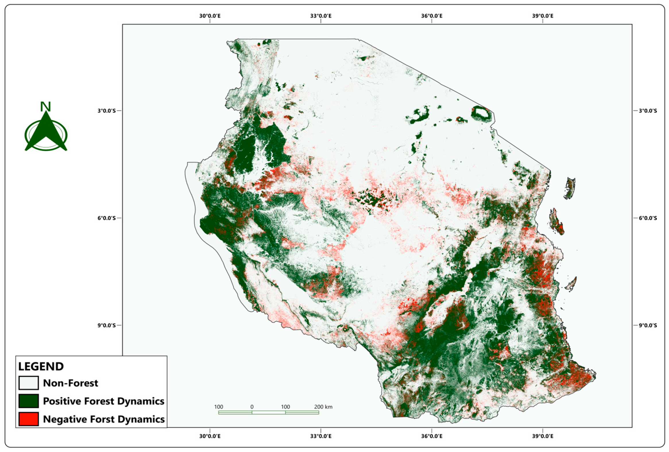
EVI was derived from MODIS MOD13Q1 products processed in Google Earth Engine. EVI was computed using the near-infrared, red, and blue bands following the standard formulation. The MODIS image collection was filtered for the study period, and scale factors were applied to convert digital values to surface reflectance. Each image was assigned temporal attributes (year and month) based on acquisition metadata, enabling the construction of a structured time series. Monthly composites were generated by grouping observations by year and month and computing mean values, reducing noise from cloud contamination and atmospheric variability. This resulted in a continuous monthly EVI time series. Forest-specific vegetation dynamics were extracted by applying a forest mask derived from the Hansen Global Forest Change dataset using a 30% tree cover threshold for the year 2000. This ensured that only forested pixels were included, while non-forest areas were excluded through spatial masking. Finally, mean EVI values were computed for forested areas within the national boundary of Tanzania for each monthly composite, producing a consistent time series for analyzing forest dynamics over time.

To address seasonal variation driven by rainfall and phenological cycles unrelated to forest cover change, the raw monthly EVI series is deseasonalized prior to analysis equivalent to computing EVI anomalies [39,46,47]. This procedure eliminates recurring seasonal fluctuations, accounts for inherent differences in baseline greenness across vegetation types, and allows the analysis to focus on inter-annual variability and structural changes in forest cover rather than predictable seasonal cycles. The deseasonalized EVI series used in the VAR model therefore reflects genuine deviations from expected seasonal vegetation patterns, attributable to underlying changes in forest conditions rather than normal seasonal variation in greenness.

3.4. Econometric Approach

Following [32,33,48,49], our study employs a VAR model to analyze the dynamic interrelationships between fiscal policy variables and forest cover conditions and dynamics in Tanzania from January 2001 to December 2024. The VAR framework is appropriate as it captures feedback effects and temporal dynamics among macroeconomic and environmental variables without imposing strong a priori theoretical restrictions.

Unlike [32,48], who estimate their VAR models in demeaned form, this study retains a constant term in the specification. The inclusion of the constant captures the average level of the variables over time and ensures unbiased estimation, given that the variables are not mean zero processes.

The general reduced form VAR model is specified as follows:

$${\mathrm{Z}}_{\mathrm{t}} = {\mathrm{B}}_0 + {\mathrm{B}}_1{\mathrm{Z}}_{\mathrm{t}-1} + {\mathrm{B}}_2{\mathrm{Z}}_{\mathrm{t}-2}\dots {\mathrm{B}}_{\mathrm{p}}{\mathrm{Z}}_{\mathrm{t}-\mathrm{p}} + {\mathsf{\epsilon }}_{\mathrm{t}}$$

(3)

where

Z_t is a vector containing the endogenous variables.

B₀ is a vector of constants.

B₁, B₂, …, B_p are coefficient matrices capturing the lagged interdependencies among the variables.

ε_t is a vector of reduced form innovations (white-noise disturbances).

The vector Z_t in the VAR specification contains macroeconomic and forest cover conditions variables relevant to Tanzania.

In the base model, Z_t includes development government expenditure, total tax revenue, trade and export performance, and the Forest Cover Conditions. This specification focuses on aggregate fiscal policy variables and their interaction with overall economic activity in influencing forest cover conditions and dynamics.

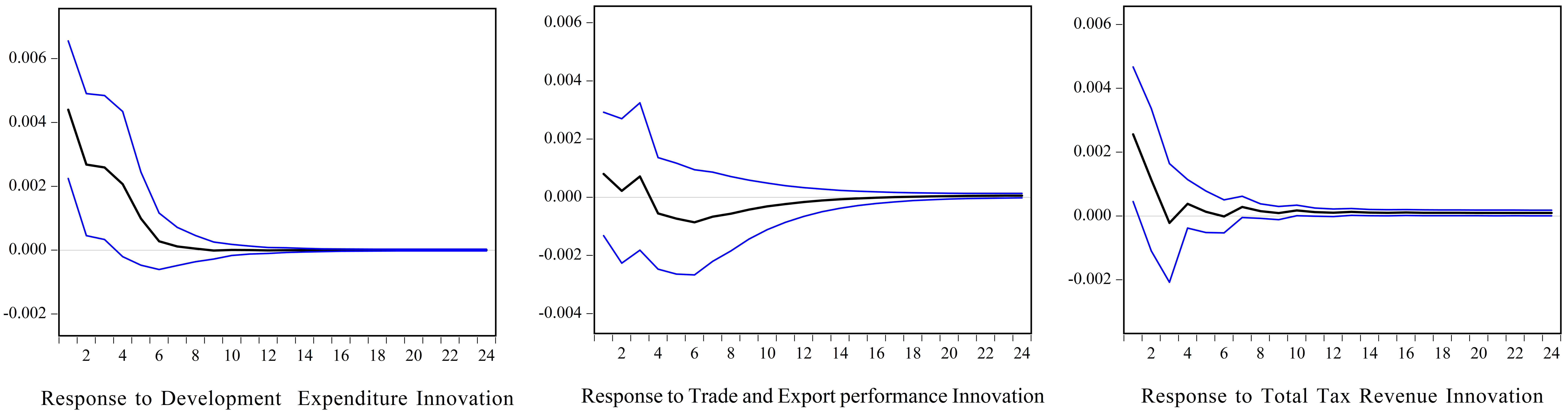
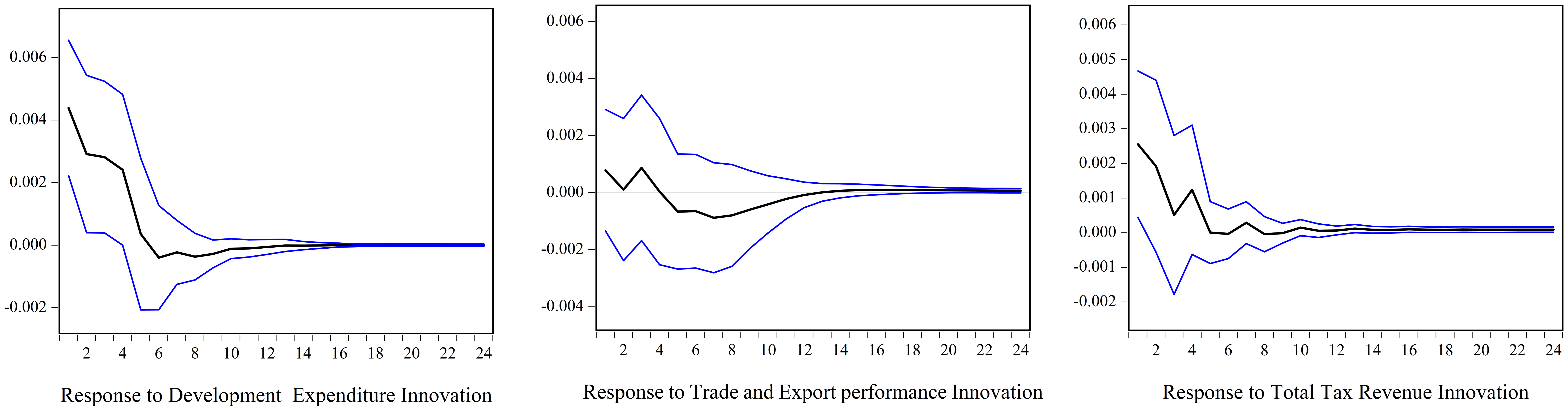
In the final part, the joint effects of government expenditure and taxation on forest cover conditions are examined under two alternative fiscal policy scenarios. The first scenario captures a deficit driven fiscal stance, where an increase in government expenditure is accompanied by a reduction in tax revenue. This represents an expansionary policy financed through fiscal imbalances. In contrast, the second scenario reflects a balanced budget approach, in which an increase in government expenditure is matched by a corresponding increase in tax revenue, maintaining fiscal neutrality. Within the VAR framework, these scenarios are implemented through simultaneous shocks to expenditure and tax variables, with the direction of the shocks distinguishing the two regimes. This approach allows the analysis to isolate how different fiscal policy combinations influence forest cover conditions and dynamics.

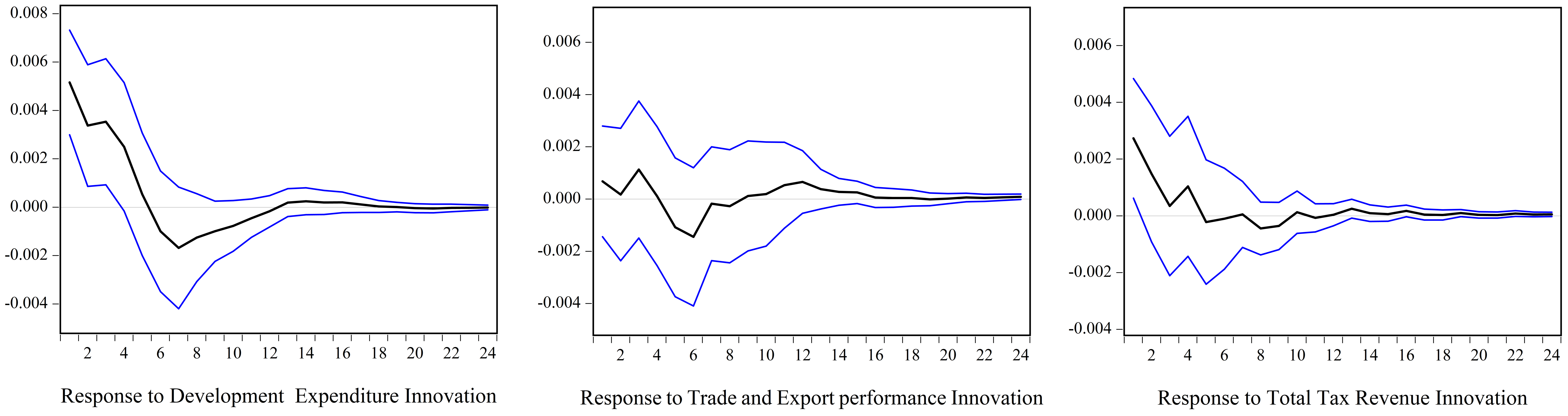
Impulse response analysis captures the extent and duration of each variable’s reaction to innovations elsewhere in the system. As emphasized in the time-series literature [50], the residuals obtained directly from a reduced-form VAR cannot be interpreted as independent shocks, since each one reflects a mixture of the true underlying structural disturbances. To address this, the covariance matrix of the reduced-form residuals is decomposed using the Cholesky method, producing a set of orthogonal shocks that can be meaningfully attributed to individual variables. This procedure depends on assigning a specific causal ordering to the variables included in the system. Here, the variables are arranged as development expenditure, trade and export performance, tax revenue, and forest cover conditions. Under this arrangement, development expenditure shocks are treated as fully exogenous within the month, trade and export performance may react immediately only to fiscal spending, tax revenue can respond to both fiscal and trade innovations, and forest cover placed last is allowed to adjust contemporaneously to shocks originating from all three preceding variables. A similar logic underlies the identification strategy adopted for Brazilian deforestation study, where government expenditure, output, tax revenue, and deforestation are ordered analogously to isolate fiscal shocks [33].

To evaluate whether this specific sequencing drives the results, three alternative orderings were also estimated, placing trade and export performance ahead of development expenditure and tax revenue; placing trade and export performance ahead of tax revenue and development expenditure; and placing tax revenue first, followed by trade performance and development expenditure. Across all three alternatives, the estimated dynamics remained essentially unchanged, indicating that the identification scheme is not driving the substantive conclusions (full results available upon request).

4. Results and Discussion

The estimation model was specified to examine the relationship between fiscal policy and forest cover conditions and dynamics. In this model, overall development government expenditure and total tax revenue are incorporated separately to account for different fiscal regimes, including balanced and deficit positions. This specification allows for a more comprehensive assessment of the relationship between fiscal policy and EVI-based forest cover conditions by capturing both the individual and joint effects of fiscal policy variables on forest cover conditions over time.

4.1. Model Specification and Pre-Estimation Tests

Prior to model estimation, the time-series characteristics of all variables included in the analysis were assessed to ensure correct model specification and to prevent the occurrence of spurious relationships. This was done using the Augmented Dickey–Fuller (ADF) and Phillips–Perron (PP) unit root tests, with the corresponding outcomes reported in

Table 2. Stationarity Test Results for the Variables.

		ADF		Phillips-Perron
Variables	Deterministic	Level	Difference	Level	Difference
Forest Cover Conditions (EVI)	Intercept	−9.268(0) ***		−9.266(5) ***
	Trend and intercept	−9.581(0) ***		−9.131(8) ***
Development Government Expenditure	Intercept	−0.496(11)	−9.653(10) ***	−5.726(10) ***	−133.7(146) ***
	Trend and intercept	−15.31(0) ***	−9.619(10) ***	−15.32(1) ***	−134.5(148) ***
Total Tax Revenue	Intercept	−2.789(5) *	−24.71(1) ***	−1.600(34)	−35.22(70) ***
	Trend and intercept	−0.864(5)	−11.87(1) ***	−3.772(40) **	−47.30(56) ***
Trade and Export performance	Intercept	−1.394(10)	−5.524(12) ***	−1.653(16)	−35.13(31) ***
	Trend and intercept	−1.965(10)	−5.534(12) ***	−5.432(1) ***	−35.33(31) ***

Note: *, **, *** stand for statistical significance at 10%, 5% and 1%, respectively; Numbers in parentheses show lag lengths, selected using the Schwarz Bayesian Criterion for the ADF tests and the Newey–West method for the PP tests.

. Each test was implemented under two specifications: one including only a constant term, and another incorporating both a constant and a deterministic trend to account for different data generating processes.

The Phillips–Perron test serves as a robustness check for the ADF approach, as it adjusts for serial correlation of higher order and remains reliable in the presence of heteroskedasticity and possible structural shifts. The lag structure was selected based on the Schwarz Information Criterion (SIC), ensuring an optimal balance between fit and parsimony.

The findings reveal that the variables exhibit mixed integration properties, with some being stationary at level form I(0), while others achieve stationarity only after first differencing I(1). This combination of integration orders indicates heterogeneous time-series characteristics among variables.

The lag length selection was guided by the Akaike Information Criterion (AIC), Schwarz Information Criterion (SIC), and Hannan–Quinn Information Criterion (HQIC). Although the information criteria suggested optimal lag lengths of 3 and 6, a lag length of 6 was ultimately selected, as it adequately eliminated serial correlation in the residuals. This choice is consistent with standard VAR practice, where diagnostic checks are prioritized to ensure model validity [50,51]. The selected lag structure was therefore adopted for all subsequent estimations.

Preceding the estimation process, the Johansen cointegration test was conducted to determine the number of cointegrating relationships among the series, with results cross validated using both the trace and maximum eigenvalue tests (Appendix A 

Table A3. Johansen Cointegration Rank Test Results.

3 Lags
Hypothesized No. of CE(s)	Eigenvalue	Trace Statistic	0.05 Critical Value	Prob.	Max-Eigen Statistic	0.05 Critical Value	Prob.
None	0.198099	111.0797	29.79707	0.0000	62.69870	21.13162	0.0000
At most 1	0.145168	48.38098	15.49471	0.0000	44.54548	14.26460	0.0000
At most 2	0.013414	3.835498	3.841465	0.0502	3.835498	3.841465	0.0502
6 Lags
Hypothesized No. of CE(s)	Eigenvalue	Trace Statistic	0.05 Critical Value	Prob.	Max-Eigen Statistic	0.05 Critical Value	Prob.
None	0.100225	52.36612	29.79707	0.0000	29.67653	21.13162	0.0025
At most 1	0.065178	22.68958	15.49471	0.0035	18.93926	14.26460	0.0085
At most 2	0.013258	3.750321	3.841465	0.0528	3.750321	3.841465	0.0528

Note: Both trace and max-eigenvalue tests indicate at most 2 cointegrating equations at the 0.05 level.

). The test confirmed the presence of at most two cointegrating vectors, supporting the use of a Vector Error Correction Model (VECM) as the baseline specification, which explicitly captures both short-run dynamics and long-run equilibrium adjustment among the variables.

Given that the Johansen cointegration test confirmed cointegrating vectors among the variables, a VECM was estimated as the baseline specification, jointly capturing short-run dynamics and long-run equilibrium adjustment. To complement this, a VAR in levels was additionally estimated, from which IRFs and FEVD were derived to assess the dynamic effects of fiscal policy shocks on forest cover over time. (Full VECM results are available upon request).

This approach is justified in line with [52], who argues that VARs in levels remain appropriate for analyzing dynamic relationships without imposing restrictive prior assumptions, and ref. [50], who shows that VARs in levels yield consistent impulse response estimates provided the system is stable. Further support comes from [53] provide foundational support, asserting that the presence of unit roots among variables does not invalidate the estimation of a VAR in levels, thus lending additional theoretical grounding to the analytical framework employed in this study.

The stability of the estimated VAR model was assessed to ensure that the system is well-behaved. Following [50,51], a VAR is considered stable if all eigenvalues of the companion matrix lie strictly within the unit circle. Stability guarantees a valid infinite-order vector moving average representation, which is a necessary condition for the meaningful interpretation of IRFs and FEVD. The inverse roots of the Autoregressive (AR) characteristic polynomial, presented in Appendix A Figure A1, all lie strictly inside the unit circle, confirming that the estimated VAR model satisfies the stability condition and that the estimated responses to shocks are both reliable and interpretable.

Serial autocorrelation in the VAR model residuals was examined using both the Lagrange Multiplier (LM) test and the Portmanteau test, following two complementary approaches. Panel A tests for autocorrelation at each individual lag h, providing a targeted assessment of residual behavior at each specific horizon, while Panel B tests sequentially from lag 1 to h, offering a comprehensive evaluation of residual autocorrelation across all lags up to the chosen horizon. Together, these two approaches provide a robust assessment of the model’s residual properties, as recommended by [50]. As reported in Appendix A 

Table A1. LM Test Results for Serial Correlation in VAR Residuals.

Panel A: No Serial Correlation at Lag h
Lag	LRE Stat	Df	Prob.	Rao F-Stat	Df	Prob.
6	14.94489	16	0.5287	0.934604	(16, 764.4)	0.5287
Panel B: No Serial Correlation at Lags 1 to h
Lag	LRE Stat	Df	Prob.	Rao F-Stat	Df	Prob.
1	18.09480	16	0.3184	1.133909	(16, 764.4)	0.3184
2	24.67815	32	0.8189	0.768894	(32, 908.8)	0.8189
3	48.17539	48	0.4657	1.004606	(48, 934.2)	0.4661
4	58.76234	64	0.6616	0.916281	(64, 934.0)	0.6623
5	83.32299	80	0.3776	1.043863	(80, 925.5)	0.3790
6	104.7181	96	0.2550	1.096101	(96, 913.7)	0.2570

Note: A p-value greater than 0.05 indicates no significant autocorrelation.

, the p-values across all lags under both Panels A and B of the LM test exceed the 5% significance level, confirming that the residuals of the VAR model are free from serial correlation at all tested lags. This result is further corroborated by the Portmanteau test, reported in Appendix A 

Table A2. VAR Residual Portmanteau Tests for Autocorrelation. Null Hypothesis: No residual autocorrelations up to lag h.

Lags	Q-Stat	Prob.	Adj Q-Stat	Prob.	df
1	0.612896	---	0.615077	---	---
2	1.422018	---	1.429978	---	---
3	3.271888	---	3.299739	---	---
4	5.122287	---	5.176763	---	---
5	7.451295	---	7.547811	---	---
6	13.75161	---	13.98509	---	---
7	19.47747	0.2447	19.85670	0.2267	16

Note: A p-value greater than 0.05 indicates no significant autocorrelation.

, which similarly shows p-values exceeding the 5% significance level across all tested lags. Together, these results support the adequacy of the lag structure and validate the use of the estimated model for inference.

4.2. Impulse Response and Variance Decomposition

The IRFs and Variance Decomposition jointly describe the dynamic interactions among fiscal policy, economic activity, and forest cover conditions within the VAR framework. Both analyses are based on the Cholesky decomposition of the residual covariance matrix to ensure orthogonal structural shocks. The recursive identification follows an economically motivated ordering commonly used in VAR literature, where government development expenditure is assumed not to respond contemporaneously to other shocks, while trade and export performance and total tax revenue respond sequentially, and forest cover conditions and dynamics responds contemporaneously to all fiscal and economic shocks. This approach, consistent with the empirical literature [33], facilitates meaningful interpretation of structural shocks and their transmission mechanisms.

As reported in

Table 3. Variance Decomposition of Forest Cover Conditions and Dynamics.

Period	Development Government Expenditure	Trade and Export Performance	Total Tax Revenue	Forest Cover Dynamics
1	07.75	0.14	02.17	89.94
4	12.05	0.38	02.31	85.26
8	12.70	01.05	02.26	83.99
12	12.94	01.19	02.27	83.60
24	12.95	01.25	02.29	83.51

, forest cover dynamics are predominantly explained by their own innovations in the short run, accounting for 89.94% of total variation in period 1. The contributions of development government expenditure, total tax revenue and trade and export performance are comparatively small at this stage.

As the forecast horizon increases, the findings suggest that the influence of fiscal variables becomes more substantial. Development government expenditure emerges as the dominant external driver, rising to 12.05% in period 4 and stabilizing at a consistently high level of approximately 12.95% by period 24. Total tax revenue also shows a gradual increase, while trade and export performance remains negligible.

Notably, as indicated by the FEVD, development expenditure accounts for approximately 12.95% of the variation in forest cover conditions, representing a substantial share among the explanatory variables and pointing to a relevant association between development expenditure and forest cover dynamics over the short run. This finding is broadly comparable to [33], who reports that government spending accounts for 12.58% of the FEVD in the Amazon after two years. A similar pattern is observed by [33] in the Atlantic Forest, where government spending accounts for 18.47% of the variation over the same period.

The IRFs in Figure 2, illustrate that forest cover conditions and dynamics responds differently to fiscal and economic shocks over a 24 period horizon, while the purple lines represent the ±2 standard error bands (approximately a 95% confidence interval).

Tax revenue shocks generate a positive and statistically significant response only in the first period. Thereafter, the response declines rapidly and oscillates slightly around zero, remaining statistically insignificant in subsequent periods before converging to zero in the long-run.

Development expenditure shocks produce a positive and statistically significant effect on forest cover conditions from periods 1 to 3, while the fourth period remains weakly significant at the 10% level. Afterward, the response turns negative around periods 5 to 7, before gradually recovering, crossing back toward zero around the middle periods, and eventually converging to zero.

In contrast, trade and export performance shocks remain statistically insignificant throughout the entire horizon. The response fluctuates mildly between positive and negative values before gradually converging toward zero.

Overall, our results point to a relevant short-run association between fiscal policy and forest cover conditions in Tanzania. The findings suggest that fiscal instruments, particularly revenue generation and development expenditure, are associated with favorable forest cover conditions. These results are consistent with the broader literature suggesting that fiscal policy can reduce environmental degradation through enhanced public investment [32,33,54]. Moreover, a stronger and more efficient revenue system can support environmental management by improving the government’s capacity to finance conservation and sustainable resource management initiatives [55,56,57]. They also support the view that fiscal policy plays a meaningful role in promoting sustainable environmental and natural resource outcomes.

To assess the sensitivity of the results to the choice of lag length, the VAR model was re-estimated using 2, 3, and 4 lags, in addition to the baseline specification. The resulting impulse response functions, presented in Appendix A Figure A2, Figure A3 and Figure A4, display patterns consistent across all lag specifications, with shocks producing responses of similar sign, magnitude, and persistence relative to the baseline model. These findings confirm that the main results are not driven by the specific lag length chosen and reinforce the robustness of the reported impulse responses and variance decomposition.

In the closing phase of our analysis, the combined effects of government expenditure and taxation on forest cover conditions and dynamics are examined through two fiscal policy scenarios, a deficit-financed fiscal impulse and a balanced budget approach.

The IRFs for the deficit-financed scenario (Figure 3) indicate that forest cover conditions and dynamics initially responds positively following the shock in the short run. The response later turns negative in the medium term before gradually stabilizing and converging toward zero in the long-run. Overall, the pattern suggests that deficit financing does not generate a significant effect on forest cover dynamics within the model horizon.

In contrast, the estimates for the impact of a balanced budget scenario are presented in Figure 4. The results indicate that forest cover conditions improves immediately after the shock and remains above the baseline in the short run, before turning negative in the medium term and gradually stabilizing as it converges toward zero in the long-run. The response is statistically significant during the first four periods, indicating an improvement in forest conditions. These findings suggest that, if higher public spending is offset by increased tax revenue, a balanced fiscal stance can enhance forest cover conditions and dynamics without deteriorating the fiscal position. This relationship between fiscal neutrality and forest outcomes is consistent with prior empirical evidence linking disciplined fiscal frameworks to improved environmental performance [32,33,54].

4.3. Discussion of the Results

Our results for Tanzania yield two main findings. First, development government expenditure has a positive and statistically significant short-run association with EVI-based forest cover conditions, while tax revenue shocks also show a positive and statistically significant association in the initial period, suggesting that fiscal aggregates co-move with forest cover dynamics in the short run. Second, this association appears sensitive to the financing structure of fiscal policy, with differences emerging between deficit-financed and balanced budget scenarios.

The results show that development expenditure is associated with improvements in EVI-based forest cover conditions in the short run, which is broadly consistent with evidence that public expenditure can be linked to environmental outcomes through targeted allocation and institutional support [32,33,54]. In the context of Tanzania, this suggests that the country may be more likely to observe favorable forest cover signals in the short run when increased development expenditure is directed toward environmental objectives. It further implies that fiscal resources, when efficiently allocated, could potentially serve as a relevant instrument for supporting forest cover conditions alongside broader development goals.

Our findings on the revenue side indicate a positive short-run association between tax revenue and forest cover conditions, although its contribution is relatively small, reflected in a 2% share of the FEVD. This points to a possible, modest role for domestic resource mobilization in relation to forest cover dynamics, though the transmission mechanism is not directly evidenced in the present analysis and should be treated as an area for future investigation. This interpretation is broadly in line with [55,56,57], which discuss the relevance of tax systems for environmental outcomes more generally.

The apparent divergence between deficit and balanced-budget scenarios points to an association between financing structure and forest cover dynamics, with borrowing-led expansion showing weaker and less stable patterns than domestically financed expenditure [32]. This distinction matters because it suggests that the source of financing, and not merely the scale of expenditure, shapes how fiscal policy relates to environmental outcomes in practice. Fiscal expansions financed through borrowing may carry additional macroeconomic pressures, such as debt servicing costs or crowding out effects that could dilute or destabilize any short-run environmental benefits associated with the underlying spending, whereas expenditure financed through domestic revenue appears to translate into comparatively steadier forest cover dynamics. Overall, the evidence for Tanzania is consistent with the broader idea that fiscal design, encompassing not only how much is spent but how that spending is financed and sustained over time, relates to forest cover dynamics in ways that go beyond expenditure magnitude alone, in line with the broader literature linking fiscal discipline to environmental performance [32,33,54,58].

Trade and export performance, included in the model primarily as a business cycle indicator, showed no statistically significant association with forest cover conditions at any lag. This contrasts with [33], who use GDP as their business cycle proxy and find that higher economic activity is associated with increased deforestation in the Brazilian Amazon and Atlantic Forest, though the effect only becomes significant several months after the initial shock. Similarly, ref. [59] examining conventional energy consumption and environmental quality in Brazil, find a positive relationship between economic growth and CO₂ emissions, reinforcing the broader pattern of business cycle activity being associated with adverse environmental outcomes in other contexts. Using trade and export performance as our business cycle proxy, no such lagged significance emerges here, suggesting that short-run business cycle fluctuations are not closely linked to forest cover conditions and dynamics in Tanzania over the horizon examined, in contrast to much of the existing literature that has emphasized trade related channels, such as agricultural export expansion, as drivers of forest pressure [11].

We conclude that fiscal aggregates and forest cover conditions in Tanzania are dynamically linked in the short run, with the strength and direction of the relationship shaped by both the timing of fiscal shocks and the underlying financing structure. This suggests that favorable forest cover signals in Tanzania are more likely to align with fiscal expansion when it is supported by sustainable financing mechanisms, including domestic revenue mobilization that can enable development expenditure alongside environmental management initiatives.

5. Conclusions and Policy Implications

Tanzania continues to experience significant pressure on its forest resources despite the existence of national and sub-national sustainable forest management policies and regulations, wood-product traceability systems, and ongoing policy interventions such as afforestation programs and REDD+ initiatives. While forests remain essential for rural livelihoods, ecosystem services, biodiversity conservation, and climate regulation, persistent pressures arising from energy demand, population growth, and land-use change continue to pose challenges for forest conditions. Although previous studies have mainly focused on drivers such as agricultural expansion and charcoal production, this study contributes to the literature by exploring the dynamic association between fiscal policy aggregates and forest cover conditions. Specifically, this study extends the environmental macroeconomic literature by using an EVI-based indicator of forest cover conditions as a proxy for environmental quality in Tanzania, thereby providing exploratory empirical evidence from a resource-dependent developing economy. We emphasize that this indicator reflects forest cover conditions rather than deforestation or forest loss directly, and the findings should be interpreted accordingly.

This study employs a VAR framework complemented by impulse response analysis to examine the short-run dynamic association between fiscal policy aggregates and forest cover conditions. The results indicate that development government expenditure shows a positive significant short-run association with EVI-based forest cover conditions, though the strength and direction of this association evolve over the medium term, with the response to development expenditure moving through a temporary negative and insignificance phase before settling back toward zero. This pattern points to a short-run, evolving relationship between public expenditure and forest cover dynamics, rather than a single, uniform trajectory of improvement.

This study further suggests that fiscal sustainability plays a relevant role in relation to forest cover conditions, with fiscally balanced conditions being associated with more stable patterns in forest cover dynamics than deficit-financed expansion. The response to a balanced-budget innovation builds significantly initially, dips mildly and become insignificant, and gradually converges toward zero. This indicates that the financing structure of public expenditure, alongside the level of spending itself, is relevant for understanding forest cover conditions in Tanzania.

From a policy perspective, the findings indicate that development government expenditure is associated with favorable forest cover conditions in Tanzania in the short run, particularly when allocated toward environmentally relevant sectors. Financing structure also matters; balanced fiscal frameworks, where expenditure is supported by sustainable domestic revenue rather than borrowing, tend to show more stable patterns in forest cover dynamics in the short run than deficit-financed expansion. This highlights the value of integrating fiscal discipline with environmental planning as part of a broader approach to natural resource management.

The analysis further suggests that fiscal policy may be more closely linked to favorable forest cover signals when development expenditure is broadly aligned with environmental objectives. Given the persistent pressure on forest resources, directing development expenditure toward measures that reduce forest pressure and promote sustainable resource use is a relevant policy direction worth pursuing. In this regard, Tanzania may support forest cover conditions through broader strategies that strengthen institutional capacity for natural resource management alongside fiscal policy design.

While this study provides empirical evidence on the association between fiscal policy instruments and forest cover dynamics in Tanzania, some limitations should be acknowledged. The national level design, necessitated by the current unavailability of district level fiscal data of sufficient length and sectoral disaggregation in Tanzania, precludes the capture of spatially heterogeneous effects across the country’s diverse forest landscapes. Nonetheless, the findings document a meaningful national-level association that establishes an important empirical foundation for future subnational and cross-country investigations in Sub-Saharan Africa.

Future research should combine subnational fiscal data with geographically disaggregated forest cover measures to exploit spatial variation across Tanzania’s diverse landscapes. Extending the analysis using panel data across African regions would improve causal identification and enhance generalizability. Further disaggregation of fiscal instruments by sector, particularly agriculture, forestry, environmental protection, and energy, would also help identify the specific channels through which fiscal policy influences forest cover dynamics more precisely.