Modeled Net Ecosystem Productivity in the Yellow River Basin: Spatiotemporal Variability and Associations with Climate Extremes Across Ecological Zones

Abstract

How modeled ecosystem carbon balance varies across the contrasting hydroclimatic zones of the Yellow River Basin, and whether its relationships with climate extremes differ among these zones, remain insufficiently understood. To address this knowledge gap, this study examined the spatiotemporal variability of modeled net ecosystem productivity (NEP) and its associations with temperature- and precipitation-extreme indices across three major ecological zones of the basin. Using satellite-derived NDVI, reanalysis climate data, and extreme climate indices for 2000–2022, we estimated NEP from CASA-simulated net primary productivity and modeled heterotrophic respiration, and assessed its temporal trends and climatic associations across three ecological zones. Three principal findings were obtained: (1) Over the 23-year study period, basin-wide NEP showed a statistically significant increasing tendency (β = 2.699 g C m⁻² a⁻¹), with a well-defined spatial gradient characterized by relatively lower productivity in the northwestern areas and elevated productivity toward the southeastern regions. (2) Modeled NEP increased across all four seasons. Summer showed the largest positive trend, whereas autumn and winter remained net carbon-release seasons but became progressively less negative over the study period. (3) The statistical associations between modeled NEP and extreme climate indices varied markedly across ecological zones. Extreme-precipitation indices were generally positively associated with modeled NEP in the arid northwestern zone, whereas several extreme-temperature indices showed predominantly negative associations in the northeastern monsoon-influenced region. Collectively, these findings provide model-based evidence of spatially differentiated associations between ecosystem carbon balance and climate extremes across the YRB, supporting regional ecosystem assessment and climate-adaptation planning.

1. Introduction

As one of China’s most ecologically significant river systems, the Yellow River Basin (YRB) harbors a diverse array of vegetation communities, ranging from upland forests and alpine meadows to lowland wetlands and rain-fed croplands. This ecological diversity underpins the basin’s pivotal role in national carbon budgeting and positions it as a priority region for achieving China’s dual carbon neutrality commitments [1]. Accelerating climate warming has substantially elevated the occurrence of hydrometeorological extremes across the basin, including intensified drought episodes, anomalous heat events, and episodic torrential rainfall. The cascading consequences of such disturbances—vegetation dieback, heightened fire susceptibility, and net carbon release—have progressively tightened the coupling between ecosystem carbon balance and regional climate trajectories [2,3]. Spanning humid, semi-humid, semi-arid, and arid environments, the YRB exhibits pronounced spatial gradients in water availability, temperature, and vegetation conditions. Consequently, ecosystem responses to climatic disturbances differ substantially across the basin [1,4]. Meanwhile, land-use change and major function-oriented zoning have contributed to spatially heterogeneous changes in ecosystem carbon storage [5], while large-scale ecological restoration programs have promoted vegetation greenness and productivity in parts of the basin [6]. Vegetation restoration and climate variability have acted simultaneously across the basin, producing uneven changes in ecosystem carbon exchange among subregions. Clarifying how net ecosystem productivity (NEP) varies across space and over time, and how these variations are associated with climate extremes, is therefore necessary for improving regional carbon balance assessments and supporting zone-specific land-management decisions.

Net ecosystem productivity (NEP) is one measure of ecosystem carbon balance and is commonly defined as the difference between gross primary productivity (GPP) and total ecosystem respiration (ER). Equivalently, NEP can be expressed as net primary productivity (NPP) minus heterotrophic respiration (Rh) [7,8]. In this study, NEP was not directly measured but was estimated from CASA-simulated NPP and empirically modeled Rh; therefore, the resulting indicator is referred to as modeled NEP throughout the manuscript. Spatiotemporal patterns of carbon sink dynamics have been systematically examined across a hierarchy of spatial scales over recent decades, encompassing global [9], hemispheric [10,11], national [12,13], and catchment-level [4,14] perspectives, through the combined application of eddy-covariance measurements, process-oriented biogeochemical models, and satellite remote sensing. Yet, the growing frequency and intensity of extreme climatic episodes have exposed fundamental limitations in conventional modeling paradigms: analytical frameworks anchored primarily to mean temperature (TEM) and precipitation (PRE) often prove insufficient for capturing the full spectrum of ecosystem responses to abrupt environmental perturbations [15].

Against this backdrop, vapor pressure deficit and solar radiation are relevant atmospheric variables for terrestrial carbon exchange. Vapor pressure deficit (VPD) represents atmospheric evaporative demand and can influence stomatal conductance, transpiration, and photosynthetic carbon uptake. However, vegetation water-use efficiency is also regulated by soil moisture availability, stomatal behavior, vegetation characteristics, and other physiological and environmental factors [16,17,18]. Solar radiation (RADI) influences canopy energy balance and the availability of photosynthetically active radiation [19]. Across drought-prone and moisture-limited regions within the YRB, chronically elevated VPD has been shown to simultaneously inhibit soil heterotrophic respiration (Rh) and reduce vegetation carbon uptake [18,20], while interannual fluctuations in RADI propagate through light-use efficiency (ε) and photosynthetically active radiation (PAR) pathways to reshape NEP trajectories [19,21]. Beyond these gradual climatic influences, episodic extreme events—including heatwaves, prolonged droughts, and high-intensity precipitation—can trigger acute metabolic disruptions in vegetation by amplifying or interacting with prevailing meteorological conditions, with cumulative consequences for the basin’s long-term carbon sequestration capacity [22,23,24].

Previous studies in the Yellow River Basin have documented pronounced spatiotemporal variations in vegetation net primary productivity and NDVI, as well as spatially heterogeneous relationships with temperature, precipitation, and sunshine duration [4,25]. Recent studies have also examined land-use transitions, habitat-quality dynamics, and the combined effects of natural and socioeconomic drivers [26,27], while Geodetector has increasingly been used to assess the explanatory effects of individual spatial factors and their interactions [28]. However, these studies have mainly focused on vegetation productivity, greenness, land-use patterns, or habitat quality rather than ecosystem carbon balance. It therefore remains unclear whether modeled NEP exhibits consistent long-term changes across the contrasting monsoon, arid, and alpine ecological zones of the YRB, and how its spatial variability is statistically associated with multiple extreme-temperature and extreme-precipitation indices, both individually and interactively.

Building on this context, the present study estimated NEP across the YRB for the period of 2000–2022 by integrating satellite-derived NDVI observations, ERA5-Land atmospheric reanalysis data, and gridded extreme climate indices within a CASA-based modeling framework [29,30]. The analysis was conducted separately for three ecological zones with contrasting hydroclimatic conditions. Here, climate extremes refer to the selected temperature- and precipitation-extreme indices defined in Section 2.3.2. Specifically, this study aimed to: (1) characterize the spatial patterns and temporal trends of NEP at the basin scale and within each of the three ecological zones defined in Section 2.1; (2) determine how the direction and strength of the associations between NEP and extreme-temperature and precipitation indices differ among ecological zones; and (3) identify which individual and interacting climate-extreme indices explain the largest proportion of spatial variability in NEP. These questions were addressed using trend analysis, pixel-wise correlation analysis, and the Geodetector framework. By distinguishing these statistical relationships among monsoon, arid, and alpine ecological zones, this study provides a spatially differentiated perspective on regional ecosystem carbon balance in relation to extreme-temperature and precipitation indices.

2. Materials and Methods

2.1. Study Area

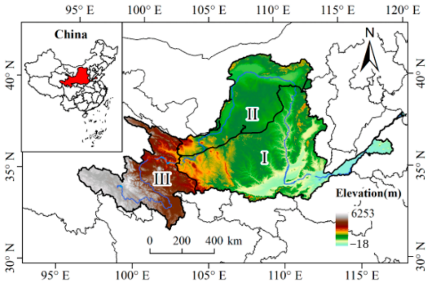
According to the ecological regionalization dataset described in Section 2.2, the Yellow River Basin was divided into three major ecological zones that served as the primary spatial analytical units in this study: Zone I, the East Asian Monsoon Ecological Zone; Zone II, the Western Arid Ecological Zone; and Zone III, the Qinghai–Tibet Alpine–Polar Ecological Zone. These zones correspond to the Roman numerals I–III shown in Figure 1 and exhibit pronounced differences in elevation, hydroclimatic conditions, and vegetation characteristics. Geographically, the basin spans northern China between 32° and 42° N and between 96° and 119° E, with the headwaters originating at the southern margins of the Bayan Har Mountain range on the Qinghai–Tibet Plateau.

The river traverses nine provincial-level administrative units before emptying into the Bohai Sea, covering a total channel length of approximately 5464 km and a drainage catchment of roughly 79.5 × 10⁴ km² (Figure 1). The basin’s topography descends in a stepped fashion from west to east: the uppermost reaches are dominated by high-altitude alpine meadows above 4200 m elevation; the middle section encompasses the Loess Plateau spanning elevations of 1000 to 2000 m, supporting grassland–shrubland mosaics and dryland agriculture; and the lowermost reaches transition into the low-lying North China Plain at elevations below 50 m, where intensive double-cropping agricultural systems dominate the landscape. Climatically, the basin spans a moisture gradient from relatively humid southeastern areas to drier northwestern regions, with mean annual temperatures spanning approximately −14 °C to 14 °C and annual precipitation totals varying between 200 and 800 mm.

2.2. Data Sources

A multi-source geospatial dataset was assembled for the YRB, with all input layers harmonized to a common spatial resolution of 1 km prior to annual raster generation. Vegetation-related remote-sensing inputs, comprising land-cover classification maps and time-series NDVI composites, were sourced from NASA’s EarthData repository (https://www.earthdata.nasa.gov/, accessed on 7 August 2026) with 500 m grid cells. Annual NPP estimates were extracted from the MOD17A3HGF Version 006 product (https://www.earthdata.nasa.gov/, accessed on 7 August 2026) at a spatial resolution of 500 m and used as an external benchmark to assess the spatial consistency of the CASA-simulated NPP. Because MOD17A3HGF is itself a model-derived product, this comparison was treated as a cross-product consistency assessment rather than as independent ground-based validation. Terrain data were obtained as a digital elevation model (DEM) from the Geospatial Data Cloud (https://www.gscloud.cn/, accessed on 8 August 2026) with a spatial resolution of 90 m. Meteorological forcing data were drawn from several complementary repositories. Monthly surface solar radiation (RADI), 2 m air temperature, and 2 m dew-point temperature for 2000–2022 were obtained from the ERA5-Land reanalysis dataset at a spatial resolution of 0.1°. Monthly VPD was calculated from the corresponding air-temperature and dew-point-temperature data. Monthly total solar radiation and monthly mean air temperature were used as inputs to the CASA model. Annual NEP was obtained by summing the monthly NEP estimates. Monthly VPD values were averaged to obtain annual mean VPD for comparison with annual NEP. Basin-scale gridded annual mean temperature (TEM) and precipitation (PRE) fields were retrieved from a dedicated high-altitude climate repository maintained by the Qinghai–Tibet Plateau research community (https://data.tpdc.ac.cn/, accessed on 8 August 2026), with a grid spacing of 1 km. Ground-level climate observations at individual weather stations were retrieved from the HRLT compilation published by Qin et al. [31] (https://doi.org/10.1594/PANGAEA.941329; accessed on 8 August 2026). Ecological-zone boundaries were delineated according to the China Ecosystem Assessment and Ecological Security Database [32] (https://www.ecosystem.csdb.cn/ecoass/ecoplanningzone_list.jsp?func=1, accessed on 8 August 2026), which partitions the YRB into 14 ecologically distinct subregions. All raster datasets were projected to a common coordinate system and aligned to a 1 km analysis grid with a consistent spatial extent and cell origin. Continuous ERA5-Land meteorological variables at approximately 0.1° spatial resolution were resampled to the target grid using bilinear interpolation. Finer-resolution continuous datasets, including the 500 m MODIS products and the 90 m DEM, were aggregated to 1 km using the mean value of the contributing pixels. The 1 km gridded temperature and precipitation datasets were retained at their original spatial resolution and aligned to the common grid. Categorical land-cover and ecological-zone datasets were resampled using the nearest-neighbor method to preserve the original class labels. The resampling of ERA5-Land data to 1 km was performed solely for spatial alignment and did not increase their effective spatial information.

2.3. Methods

The analytical framework of this study comprised three sequential components. First, satellite-derived NDVI, land-cover data, and ERA5-Land meteorological variables were integrated within the CASA–Rh framework to estimate monthly NPP, Rh, and modeled NEP, which were subsequently aggregated to seasonal and annual scales. Second, spatial mapping, Theil–Sen slope estimation, and Mann–Kendall testing were used to characterize the spatial patterns and temporal variability of modeled NEP at the basin and ecological-zone scales. Third, pixel-wise correlation analysis and Geodetector were applied to examine the statistical associations of modeled NEP with individual and interacting extreme-temperature and precipitation indices. Together, these components linked model estimation, spatiotemporal characterization, and climate-association analysis within a unified analytical framework.

2.3.1. NEP Estimation Model

NEP was not obtained from a ready-made remote-sensing product. Instead, it was calculated independently for each pixel and time step as the difference between CASA-simulated net primary productivity (NPP) and empirically estimated soil heterotrophic respiration (Rh). The MOD17A3HGF NPP product described in Section 2.2 was used only as an external benchmark for evaluating the consistency of CASA-simulated NPP and was not used as an input to the NEP calculation [7]. Following the conventional ecosystem carbon balance definition [7,8], modeled NEP was calculated as follows:

$$NEP\left(x,t\right)=NPP\left(x,t\right)-R_h\left(x,t\right)$$

(1)

where $NEP(x,t)$, $NPP(x,t)$, and $R_h(x,t)$ represent net ecosystem productivity, net primary productivity, and soil heterotrophic respiration, respectively, for pixel x during period t. Positive NEP values indicate net ecosystem carbon accumulation, whereas negative values indicate net carbon release.

Monthly NPP across the YRB was simulated using the Carnegie–Ames–Stanford Approach (CASA) model originally formulated by Potter et al. [30]. The CASA model links vegetation productivity mechanistically to the product of absorbed photosynthetically active radiation (APAR) and actual light-use efficiency (ε). Following the CASA formulation proposed by Potter et al. [30], monthly NPP was calculated as follows:

$$\mathit{NPP}\left(x,t\right)=\mathit{APAR}\left(x,t\right)\times \epsilon \left(x,t\right)$$

(2)

In this expression, $APAR(x,t)$ denotes the total photosynthetically active radiation intercepted by the vegetation canopy at pixel x in month t, and $\epsilon (x,t)$ is the realized carbon conversion efficiency at the same location and time. The actual light-use efficiency $\epsilon (x,t)$ was determined by the vegetation-specific maximum light-use efficiency (${\epsilon }_{max}$) and the corresponding temperature- and moisture-stress scalars. The ${\epsilon }_{max}$ values were adopted from Zhu et al. [33] and assigned according to land-cover type; they were not recalibrated using regional eddy-covariance observations. The specific parameter values used in this study are listed in

Table 1. Vegetation-specific maximum light-use-efficiency parameters used in the CASA model.

Land-Cover Type	${\mathit{\epsilon }}_{\mathit{m}\mathit{a}\mathit{x}}$ (g C MJ−1 APAR)	Source
Deciduous needleleaf forest	0.485	Zhu et al. [33]
Evergreen needleleaf forest	0.389	Zhu et al. [33]
Deciduous broadleaf forest	0.692	Zhu et al. [33]
Evergreen broadleaf forest	0.985	Zhu et al. [33]
Mixed needleleaf–broadleaf forest	0.475	Zhu et al. [33]
Mixed evergreen–deciduous broadleaf forest	0.768	Zhu et al. [33]
Shrubland	0.429	Zhu et al. [33]
Grassland	0.542	Zhu et al. [33]
Cropland	0.542	Zhu et al. [33]
Other vegetated land	0.542	Zhu et al. [33]

.

Canopy-absorbed photosynthetically active radiation $\left(APAR\right)$ quantifies the fraction of incoming solar radiation captured by the vegetation layer. FPAR was estimated within the CASA framework rather than obtained from a ready-made satellite FPAR product. Following Zhu et al. [33], monthly FPAR was calculated by combining estimates derived from NDVI and the simple ratio vegetation index (SR):

$$FPAR\left(x,t\right)=0.5 {FPAR}_{NDVI}\left(x,t\right)+0.5{ FPAR}_{SR}(x,t)$$

$${FPAR}_{NDVI}\left(x,t\right)={\displaystyle \frac{NDVI\left(x,t\right)-{NDVI}_{i,min}}{{NDVI}_{i,max}-{NDVI}_{i,min}}}\left({FPAR}_{max}-{FPAR}_{min}\right)+{FPAR}_{min}$$

$${FPAR}_{SR}\left(x,t\right)={\displaystyle \frac{SR\left(x,t\right)-{SR}_{i,min}}{{SR}_{i,max}-{SR}_{i,min}}}\left({FPAR}_{max}-{FPAR}_{min}\right)+{FPAR}_{min}$$

$$SR\left(x,t\right)={\displaystyle \frac{1+NDVI(x,t)}{1-NDVI(x,t)}}$$

where $i$ denotes vegetation type; ${NDVI}_{i,min}$, ${NDVI}_{i,max}$, ${SR}_{i,min}$ and ${SR}_{i,max}$ are the vegetation-type-specific lower and upper limits. ${FPAR}_{min}$ and ${FPAR}_{max}$ were set to 0.001 and 0.95, respectively [33]. Following the CASA-based APAR formulation [30,33], the resulting FPAR was used to calculate APAR as follows:

$$\mathit{APAR}\left(x,t\right)=\mathit{RADI}\left(x,t\right)\times \mathit{FPAR}\left(x,t\right)\times 0.5$$

(3)

where $RADI\left(x,t\right)$ denotes total surface solar radiation, $FPAR(x,t)$ represents the vegetation absorption fraction estimated from NDVI and vegetation type, and 0.5 is the coefficient used to convert total solar radiation to photosynthetically active radiation.

Soil heterotrophic respiration (Rh) was estimated using the temperature–precipitation empirical model proposed by Pei et al. [34]. The model was originally developed from field observations in an alpine steppe on the Qinghai–Tibet Plateau, where daily soil carbon emissions were related to daily mean air temperature and precipitation [34]. The Pei formulation has subsequently been applied in regional NEP studies in northwestern China [35], while related CASA–soil-respiration frameworks have also been used in the Yellow River Basin [36]. However, these applications do not constitute independent validation across the full hydroclimatic gradient of the YRB. The original calibration conditions are more representative of the alpine, arid, and semi-arid upper and northwestern basin than of the semi-humid southeastern basin. Therefore, applying a single parameterization across the entire YRB involves spatial extrapolation beyond the original calibration domain. The resulting Rh values were treated as model-based estimates, and this uncertainty was considered when interpreting the absolute magnitude and spatial variability of NEP. Following the temperature–precipitation empirical formulation of Pei et al. [34], monthly Rh was estimated as follows:

$$R_h(x,t)=0.22\times \left(\mathrm{e}\mathrm{x}\mathrm{p}\right(0.0912T\left(x,t\right))+\mathrm{l}\mathrm{n}(0.3145P(x,t)+1\left)\right)\times 30\times 0.465$$

(4)

where $T(x,t)$ and $P(x,t)$ represent the monthly mean air temperature (°C) and monthly mean precipitation (mm), respectively, for pixel x in month t. Following Pei et al. [34], the original daily soil carbon emission estimate was converted to an approximate monthly value by multiplying it by 30. The factor 0.465 represents the proportion of total soil carbon emission attributed to heterotrophic respiration reported by Pei et al. [34]. Seasonal and annual Rh were obtained by summing the corresponding monthly estimates, and annual NEP was calculated by summing the 12 monthly NEP estimates. This temporal upscaling represents an additional source of uncertainty.

Because basin-wide field or eddy-covariance observations of NEP and its components were unavailable, the resulting NEP values were treated as model-derived estimates rather than independently validated measurements.

2.3.2. Extraction of Extreme Climate Events and Estimation of Vapor Pressure Deficit

Gridded extreme climate indices across the YRB spanning 2000–2022 were computed using the RClimDex 1.0 software package, hosted and maintained by the Expert Team on Climate Change Detection and Indices (https://etccdi.pacificclimate.org; accessed on 8 August 2026). This toolkit ingests station-level daily records of maximum temperature, minimum temperature, and precipitation to generate a standardized suite of climate extremes indicators. Guided by both the climatic characteristics of the basin and the analytical objectives of this investigation, 19 indices were ultimately retained—11 capturing thermal extremes and 8 reflecting precipitation variability—selected from the globally recognized index system endorsed by the STARDEX project. The full set of selected indices and their formal definitions are presented in

Table 2. Indices of climate extremes.

Index Name	Code	Definitions	Units
Cold days	TX10P	Percentage of days when TX < 10th percentile	%
Cold nights	TN10P	Percentage of days when TN < 10th percentile	%
Warm days	TX90P	Percentage of days when TX > 90th percentile	%
Warm nights	TN90P	Percentage of days when TN > 90th percentile	%
Min Tmax	TXn	Minimum value of daily maximum temperature
Max Tmax	TXx	Maximum value of daily maximum temperature	°C
Min Tmin	TNn	Minimum value of daily minimum temperature	°C
Max Tmin	TNx	Maximum value of daily minimum temperature	°C
Cold spell duration index	CSDI	Total count of days within cold spells lasting at least 6 consecutive days when TN < 10th percentile	d
Warm spell duration index	WSDI	Total count of days within warm spells lasting at least 6 consecutive days when TX > 90th percentile	d
Diurnal temperature range	DTR	Average difference between TX and TN	°C
Very wet days	R95P	Total PRCP when RR > 95th percentile	mm
Extremely wet days	R99P	Total PRCP when RR > 99th percentile	mm
Simple daily intensity index	SDII	Total precipitation divided by the number of wet days	mm·d−1
Annual wet-day precipitation total	PRCPTOT	Annual precipitation accumulated on days receiving at least 1 mm of rainfall	mm
Annual maximum 1-day rainfall	RX1day	Largest precipitation amount recorded within any single day during a year	mm
Annual maximum 5-day rainfall	RX5day	Greatest precipitation accumulation observed over any consecutive 5-day period in a year	mm
Consecutive dry days	CDD	Longest uninterrupted sequence of days with daily precipitation below 1 mm	d
Consecutive wet days	CWD	Longest uninterrupted sequence of days with daily precipitation of at least 1 mm	d

.

2.3.3. Trend Analysis

Long-term directional changes in NEP were quantified using the Theil–Sen slope estimator [37], a rank-based non-parametric technique that derives trend magnitude as the median of all pairwise slopes within the time series. Owing to its insensitivity to distributional assumptions and resistance to the influence of outliers, this estimator is particularly well-suited to environmental datasets characterized by non-normal distributions or episodic anomalies. The Theil–Sen slope was calculated following Sen [37] as follows:

$${\beta }_{\mathrm{N}\mathrm{E}\mathrm{P}}=\mathrm{M}\mathrm{e}\mathrm{d}\mathrm{i}\mathrm{a}\mathrm{n}\left({\displaystyle \frac{X_{\mathrm{N}\mathrm{E}\mathrm{P}}\left(t_2\right)-X_{\mathrm{N}\mathrm{E}\mathrm{P}}\left(t_1\right)}{t_2-t_1}}\right)$$

(5)

where ${\beta }_{\mathrm{N}\mathrm{E}\mathrm{P}}$ denotes the interannual variation trend of NEP (g C m⁻² a⁻¹); $X_{\mathrm{N}\mathrm{E}\mathrm{P}}\left(t_1\right)$ and $X_{\mathrm{N}\mathrm{E}\mathrm{P}}\left(t_2\right)$ are the annual NEP values (g C m⁻² a⁻¹) for years $t_1$ and $t_2$, respectively, with 2000 ≤ $t_1$ < $t_2$ ≤ 2022.

The statistical significance of identified NEP trends was subsequently assessed through the Mann–Kendall (MK) test [38,39], a distribution-free hypothesis testing procedure that remains robust to data gaps and departures from normality, rendering it broadly applicable to long-term geophysical and ecological monitoring records [40]. Following Mann and Kendall [38,39], the rank statistic S was calculated as follows:

$$S={\displaystyle \sum _{i=1}^{n-1}}{\displaystyle \sum _{j=i+1}^n}\mathrm{s}\mathrm{g}\mathrm{n}\left(x_j-x_i\right)$$

(6)

where S is the cumulative rank difference statistic, sgn(·) denotes the sign function, and x_i and x_j are NEP observations for years i and j, respectively.

The corresponding standardized test statistic Z was calculated according to the Mann–Kendall procedure [38,39]:

$$Z=\left\{\begin{array}{c}{\displaystyle \frac{S}{\sqrt{D\left(S\right)}}}\left(S>0\right)\\ 0\left(S=0\right)\\ {\displaystyle \frac{S+1}{\sqrt{D\left(S\right)}}}\left(S<0\right)\end{array}\right.$$

(7)

where Z denotes the standardized statistic used to evaluate the significance of temporal trends (Z > 0 indicates an upward trend, and vice versa), and D(S) is the variance of S used to standardize it.

The Theil–Sen slope was used to summarize the overall direction and average magnitude of change during 2000–2022, rather than to assume that NEP followed a constant linear trajectory throughout the entire period. Interannual variability and possible changes in the temporal pattern were further examined using the sequential Mann–Kendall statistics.

2.3.4. Correlation Analysis

To characterize the linear statistical dependencies between NEP and individual climatic drivers across the YRB, pixel-wise Pearson correlation coefficients were computed for each climate variable–NEP pair [41,42]. The resulting coefficients range from −1 to +1, with magnitudes approaching unity reflecting increasingly strong covariation, and the algebraic sign distinguishing concordant from discordant relationships between the paired variables [43].

Pixel-wise Pearson correlation coefficients were used to describe the spatial direction and relative strength of the linear associations between annual NEP and individual extreme climate indices. Pearson correlation was retained to characterize linear relationships; however, some extreme climate indices may exhibit skewed or discrete distributions, and the annual series contains only 23 observations. Consequently, the correlation coefficients and parametric significance tests may be sensitive to non-normality, discrete values, and extreme observations and were therefore interpreted cautiously. Given the large number of pixel-level tests, correlations meeting the unadjusted threshold of p < 0.05 were interpreted with emphasis on broad and spatially coherent patterns rather than isolated significant pixels. Because common long-term trends were not explicitly removed before correlation analysis, some coefficients may partly reflect shared temporal trends. The ecological-zone patterns discussed in Section 3.3 were derived descriptively from the predominant sign and spatial clustering of the mapped coefficients rather than from formal area-weighted summaries. These methodological limitations are further discussed in Section 4.3. The analysis considered contemporaneous annual associations only; nonlinear threshold responses and lagged or legacy effects of antecedent climate extremes were not explicitly evaluated.

2.3.5. Geodetector

The Geodetector framework was applied following Wang et al. [44,45] to quantify the relative explanatory power of individual climatic factors and their pairwise interactions for the spatial variability of modeled NEP. Before the Geodetector analysis, all continuous extreme climate indices were discretized into five categories using the natural breaks (Jenks) method. The same discretization procedure and number of classes were applied consistently across the entire basin and the three ecological zones to maintain comparability. Geodetector is a non-parametric method and does not require the response and explanatory variables to follow normal distributions or to exhibit a predefined linear relationship [44,45]. Its application nevertheless requires meaningful spatial stratification, spatially aligned datasets with consistent resolution and extent, and sufficient valid observations within each stratum. Because the resulting q-values may depend on the selected discretization method and number of classes, they were interpreted as measures of relative explanatory power under the specified stratification rather than as evidence of causal effects; this methodological dependence is further acknowledged in Section 4.3. Specifically, the factor detector was used to quantify the relative explanatory power of individual extreme climate indices for modeled NEP patterns in four benchmark years (2005, 2010, 2015, and 2020). The interaction detector was used to classify pairwise relationships as nonlinear attenuation, single-factor nonlinear attenuation, dual-factor enhancement, independence, or nonlinear enhancement relative to the individual q-values (

Table 3. Interaction categories between explanatory factors.

Interaction Criterion	Mode of Interaction
$q\left(X_1\cap X_2\right)<\mathrm{M}\mathrm{i}\mathrm{n}\left[q\left(X_1\right),q\left(X_2\right)\right]$	Nonlinear attenuation
$\mathrm{M}\mathrm{i}\mathrm{n}\left[q\left(X_1\right),q\left(X_2\right)\right]<q\left(X_1\cap X_2\right)<\mathrm{M}\mathrm{a}\mathrm{x}\left[q\left(X_1\right),q\left(X_2\right)\right]$	Single-factor nonlinear attenuation
$q\left(X_1\cap X_2\right)>\mathrm{M}\mathrm{a}\mathrm{x}\left[q\left(X_1\right),q\left(X_2\right)\right]$	Dual-factor enhancement
$q\left(X_1\cap X_2\right)=q\left(X_1\right)+q\left(X_2\right)$	Independent
$q\left(X_1\cap X_2\right)>q\left(X_1\right)+q\left(X_2\right)$	Nonlinear enhancement

Note: Interaction categories and criteria were defined following Wang et al. [44,45].

).

3. Results

3.1. Model-Result Consistency Assessment

3.1.1. Comparison of CASA-Simulated NPP with MODIS NPP

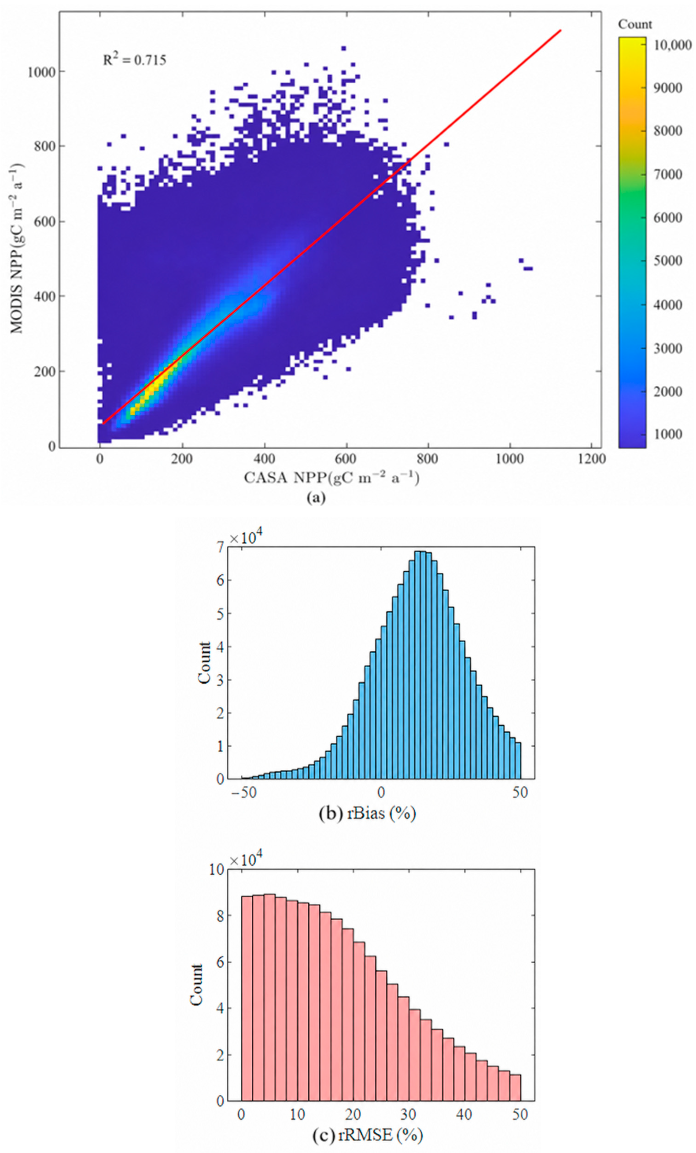
To examine whether the CASA-simulated NPP exhibited spatial consistency with an established remote-sensing NPP product, it was compared with MOD17A3HGF at a common 1 km resolution. The comparison yielded an R² of 0.715 between the two NPP datasets (Figure 2a). Pixel-level rBias and rRMSE distributions are presented in Figure 2b and Figure 2c, respectively. These results indicate broad spatial agreement between the CASA and MODIS NPP estimates. However, because MOD17A3HGF is also model-derived, this comparison represents a cross-product consistency assessment rather than an independent validation of the absolute accuracy of CASA-simulated NPP or the resulting NEP.

3.1.2. Contextual Comparison of Modeled Rh

Rh was calculated as a model-derived variable using the empirical temperature–precipitation relationship described in Section 2.3.1 [34]; therefore, its spatial and temporal variability is directly dependent on the climatic inputs and model parameterization. In the absence of basin-wide field observations, the published regional estimates presented in

Table 4. Contextual comparison of modeled heterotrophic respiration (Rh) with published regional estimates derived using different estimation approaches.

Location	Analysis Period	Rh/(g C m−2 Month−1)	Estimation Scheme	Citation
Gansu Province	2000–2010	15.19–28.00	Pei et al. [34] parameterization	[46]
Shiyang River Basin	2000–2015	11.71–38.47	Pei et al. [34] parameterization	[35]
Hexi Corridor	2001–2016	30.15–82.99	Bond-Lamberty & Raich equation	[47]
Yellow River Basin	2000–2020	3.44–30.89	Pei et al. [34] parameterization	[36]
Loess Hilly Region	August 2013	97.88	Static chamber–gas chromatography	[48]
Yellow River Basin	2000–2022	10.63–40.15	Pei et al. [34] parameterization	Present study

Note: The values are presented solely to provide contextual information on the order of magnitude of modeled Rh. Most published values were also derived from empirical or process-based models. The field-based estimate reported for the Loess Hilly Region [48] represents a site-specific measurement for August 2013 and is not directly comparable with the basin-scale, multi-year estimates in the present study.

[35,36,46,47,48] were used only to contextualize the order of magnitude of the modeled Rh values, rather than to provide independent validation of their accuracy. For the Yellow River Basin, modeled Rh ranged from 10.63 to 40.15 g C m⁻² month⁻¹ during 2000–2022. This range overlapped with the estimates reported for Gansu Province (15.19–28.00 g C m⁻² month⁻¹) by Li et al. [46] and for the Shiyang River Basin (11.71–38.47 g C m⁻² month⁻¹) by Zhang et al. [35], both of which used the Pei et al. formulation [34]. Higher values were reported for the Hexi Corridor using the Bond-Lamberty–Raich approach [47], whereas the estimate for the Loess Hilly Region was derived from short-term field measurements using static chamber–gas chromatography [48]. Published estimates for the Yellow River Basin based on the Pei et al. parameterization also showed a comparable magnitude of Rh variability [36]. Differences among studies may reflect variation in climatic conditions, vegetation cover, temporal aggregation, spatial scale, and estimation procedures. The modeled Rh values were broadly comparable in magnitude to several published regional estimates; however, this comparison should not be interpreted as independent validation.

3.2. Spatiotemporal Variability of Modeled NEP

3.2.1. Characteristics of Seasonal Changes

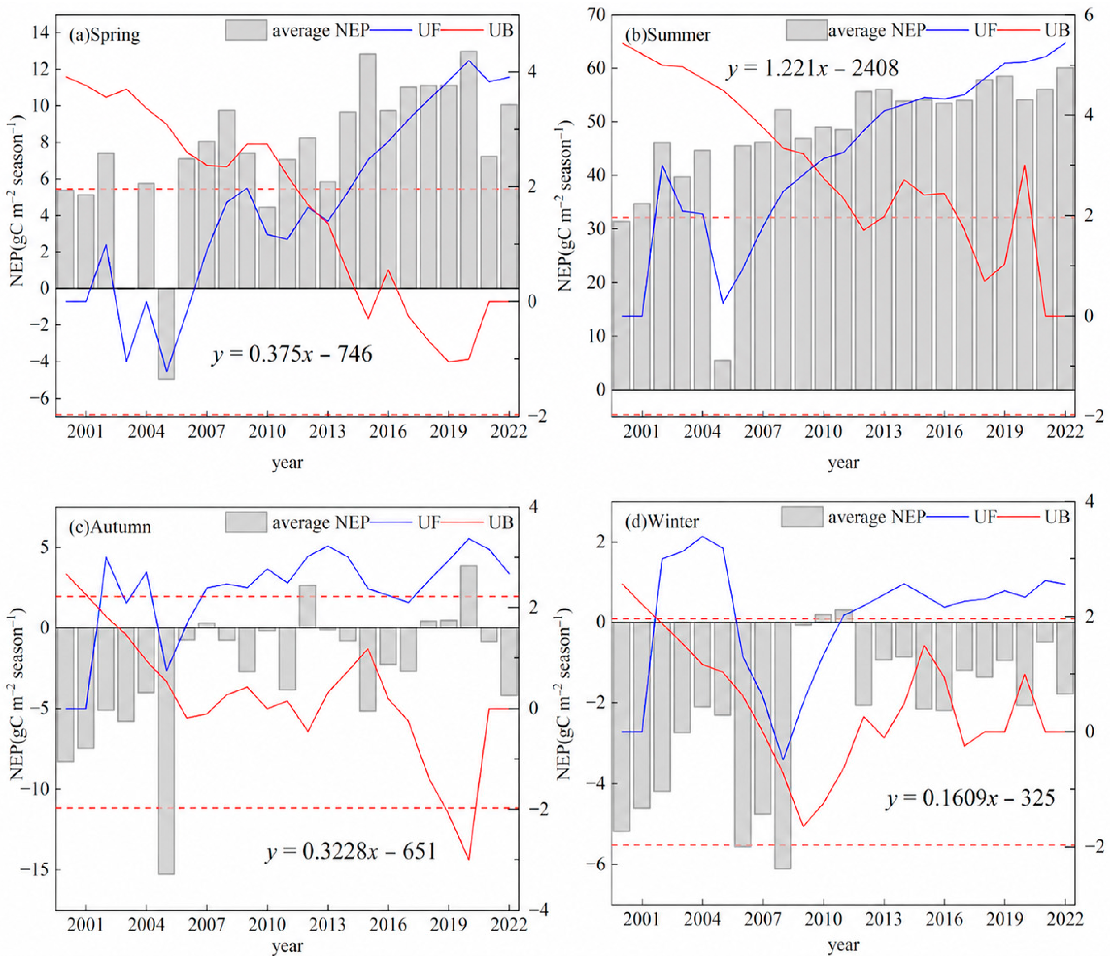
Figure 3 presents the basin-wide mean seasonal modeled NEP as an overall temporal summary. Because this spatial average integrates ecological zones with contrasting hydroclimatic and vegetation conditions, it should not be interpreted as representing uniform seasonal dynamics throughout the basin. Moreover, because the estimates were derived from CASA-simulated NPP and empirically estimated Rh, the seasonal patterns partly reflect the seasonal variability of the model inputs and parameterization. The spatial heterogeneity underlying the basin-wide mean is examined separately in Figure 4. The modeled NEP estimates showed marked intra-annual variability across the YRB, with positive values concentrated in summer and negative values occurring predominantly in autumn and winter. During 2001–2022, increasing trends in modeled NEP were observed in all four seasons (Figure 3), with the largest increase occurring in summer and a more moderate increase in spring. Although modeled NEP remained negative in autumn and winter, the values became progressively less negative over the study period. These results indicate an overall increase in modeled seasonal NEP, but their interpretation remains conditional on the structure and inputs of the CASA–Rh modeling framework.

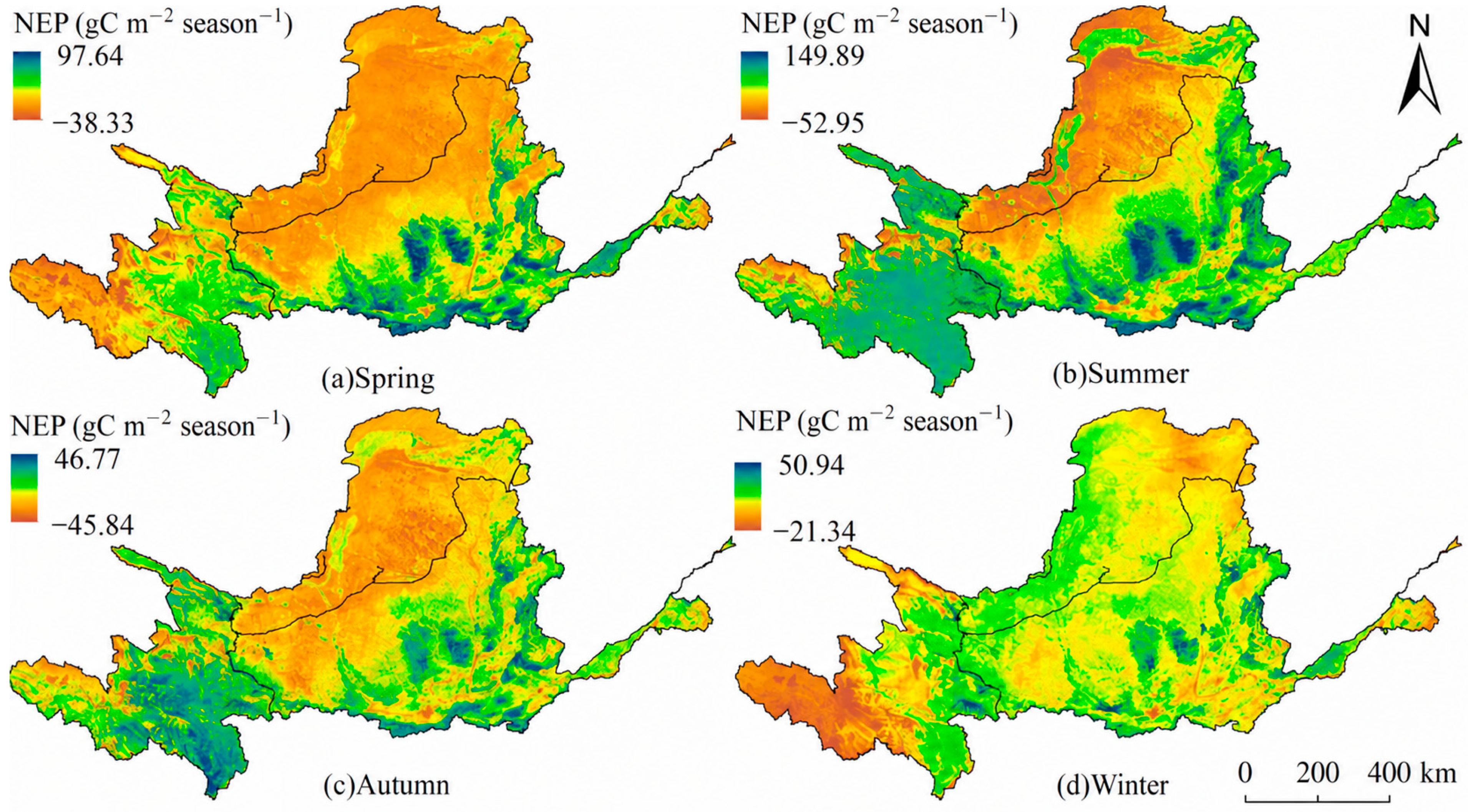
The seasonal maps further demonstrate that the basin-wide averages shown in Figure 3 conceal substantial spatial differences among the monsoon, arid, and alpine ecological zones. In spatial terms, seasonal NEP across all four seasons is organized along a broadly east-to-west decreasing gradient (Figure 4). Summer NEP reaches its peak at 48.015 g C m⁻² season⁻¹, with the highest values concentrated in the Huanglongshan-Ziwuling upland belt of the eastern monsoon zone, while the northwestern arid subregion of the basin consistently registers the lowest seasonal totals. Additionally, the Qinghai–Tibet Plateau ecological region exhibits higher summer and autumn NEP than spring and winter, which may be associated with the short growing season and temperature constraints in this high-altitude region.

3.2.2. Annual Variability and Spatial Trends

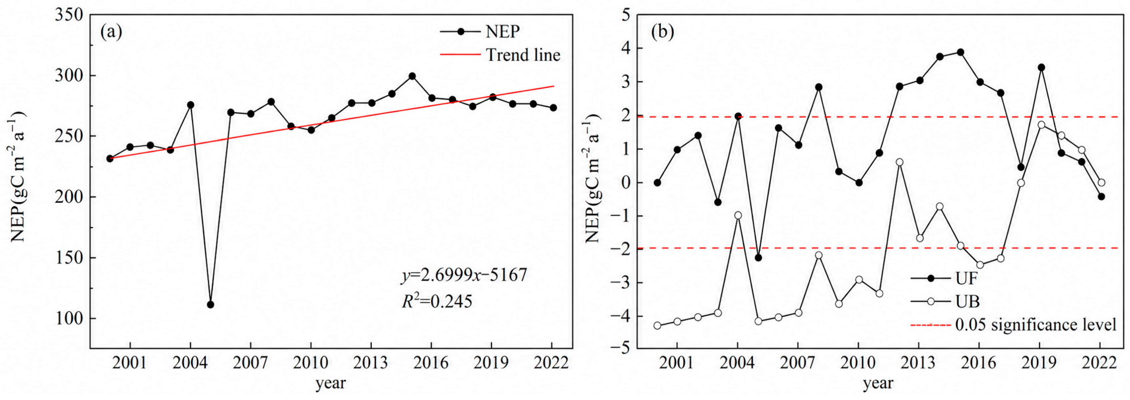
Basin-wide modeled NEP exhibited pronounced interannual variability during 2000–2022 (Figure 5a). The highest annual value was recorded in 2015 (299.863 g C m⁻² a⁻¹), whereas the lowest occurred in 2005 (110.98 g C m⁻² a⁻¹). Despite these fluctuations, the overall Theil–Sen slope was positive (β = 2.699 g C m⁻² a⁻¹, p < 0.05), indicating a long-term increasing tendency. This slope represents the average direction and magnitude of change over the full study period and does not imply a constant year-to-year increase. The forward and backward sequential Mann–Kendall curves intersected around 2020 within the 95% confidence limits (Figure 5b), suggesting a possible change in the temporal pattern of modeled NEP. This timing may reflect the combined influence of interannual hydroclimatic variability and changing vegetation conditions; however, the present analysis does not allow the possible shift to be attributed to a specific ecological driver. Therefore, the annual series is interpreted as an overall increasing tendency accompanied by substantial interannual fluctuations and temporally non-uniform variation.

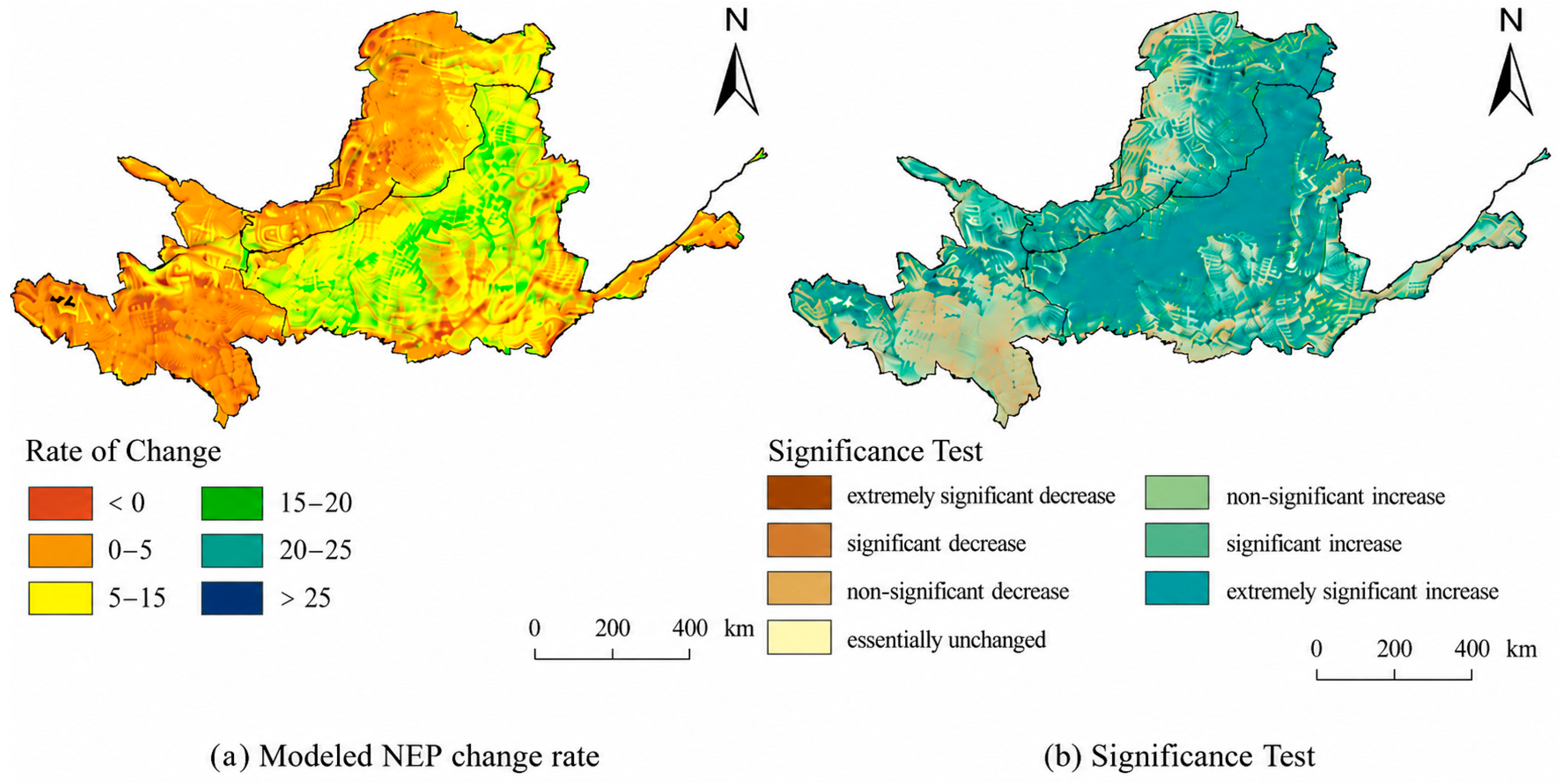
Spatially, positive modeled NEP change rates predominated across the basin, particularly in the eastern and central regions (Figure 6a). Figure 6b combines the direction of the Theil–Sen slope (β) with the significance level of the Mann–Kendall statistic (Z); it therefore represents a classification of both trend direction and statistical significance. As summarized in

Table 5. Classification and areal proportions of modeled NEP trends based on the sign of the Theil–Sen slope and the Mann–Kendall significance statistic in the YRB and its three ecological zones during 2000–2022.

β	|Z|	Trend of NEP	Areal Share of Each NEP Trend Class (%)
			I	II	III	YRB
>0	2.58 < |Z|	Extremely significant increase	64.84	47.67	22.51	49.43
	1.96 < |Z| ≤ 2.58	Significant increase	9.97	12.50	10.97	10.88
	|Z| ≤ 1.96	Non-significant increase	20.69	30.68	48.29	30.42
=0	|Z|	Essentially unchanged	0.52	1.23	3.08	1.37
<0	|Z| ≤ 1.96	Non-significant decrease	3.19	7.08	14.74	7.19
	1.96 < |Z| ≤ 2.58	Significant decrease	0.31	0.40	0.24	0.31
	2.58 < |Z|	Extremely significant decrease	0.48	0.45	0.17	0.40

, increasing trends accounted for 90.73% of the basin area, including 49.43% with an extremely significant increase, 10.88% with a significant increase, and 30.42% with a non-significant increase. In contrast, decreasing trends accounted for only 7.90% of the basin area. Thus, Figure 6a,b consistently indicate an increase-dominated spatial pattern. Zone I recorded the highest proportion of areas exhibiting an extremely significant increasing trend in modeled NEP (64.84%), followed by Zone II (47.67%) and Zone III (22.51%), indicating that the spatial extent of strongly increasing trends generally declined from the eastern monsoon zone toward the western arid and alpine zones.

3.3. Associations Between Extreme Climate Indices and NEP

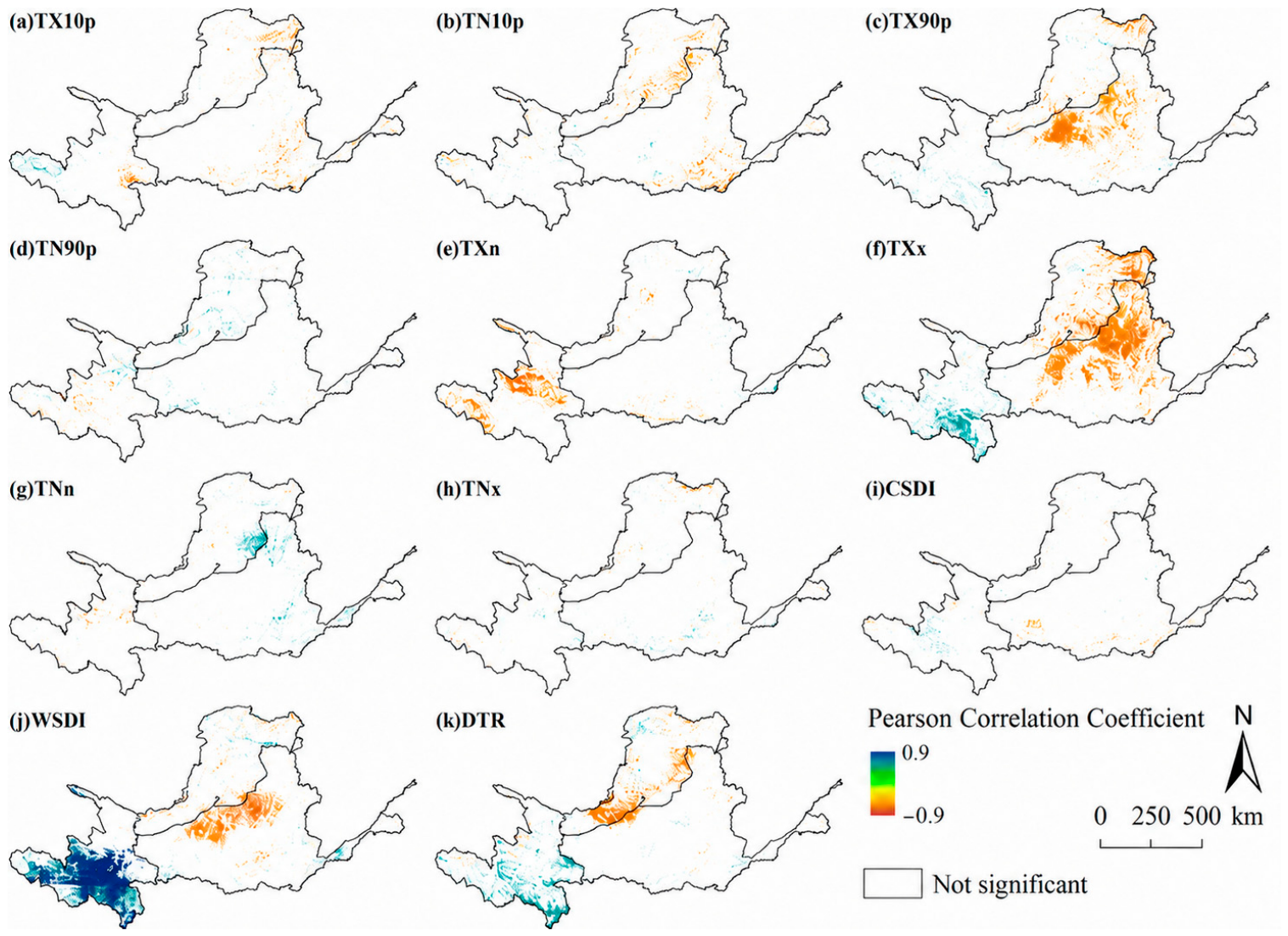
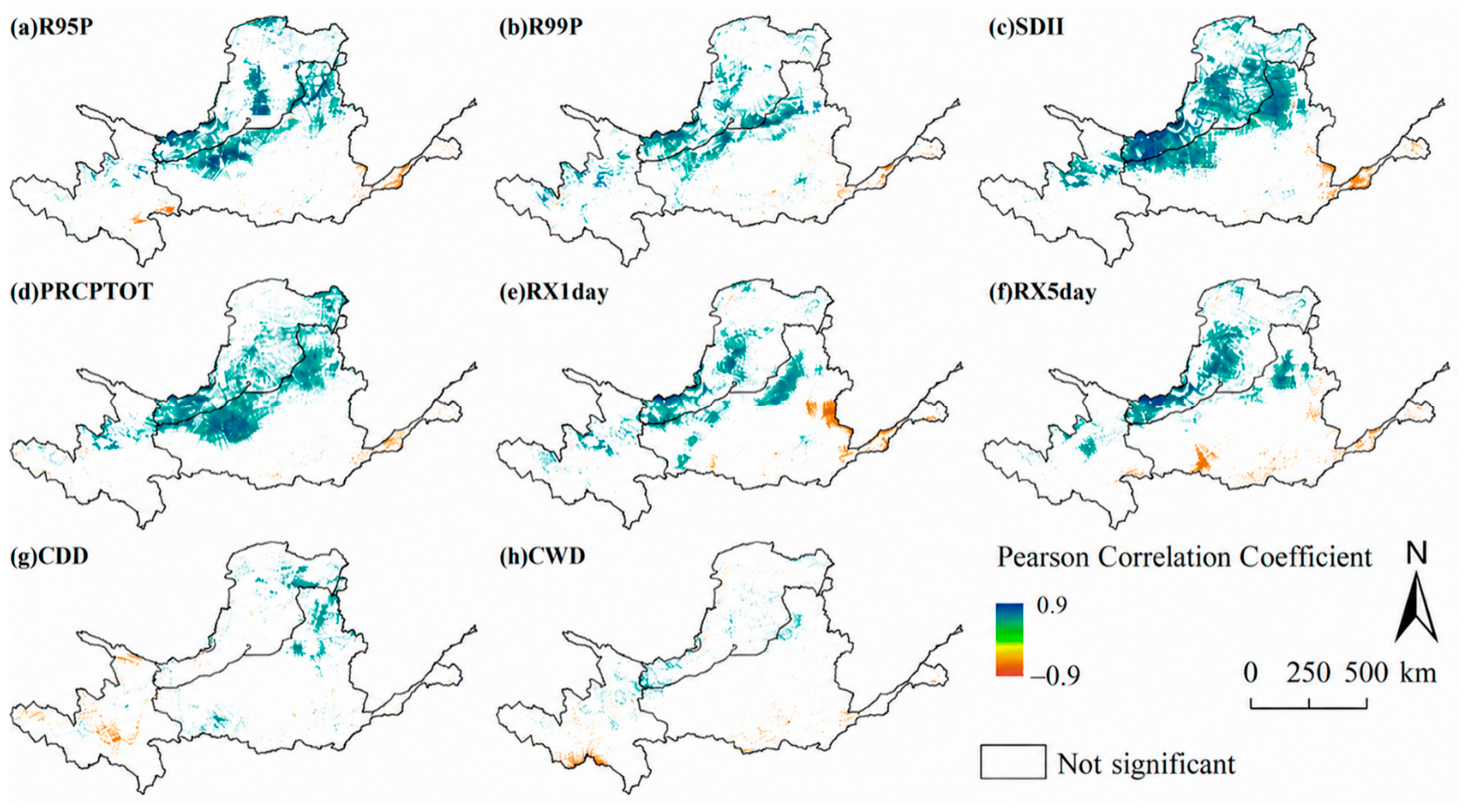
The following Pearson correlation maps are interpreted as descriptive representations of linear association patterns; they should not be regarded as distribution-robust estimates for all extreme climate indices. Across the 2000–2022 study period, the direction and magnitude of the statistical associations between modeled NEP and extreme climate indices varied considerably among the three ecological zones. Pixel-wise Pearson correlation analysis revealed spatially heterogeneous associations between modeled NEP and extreme-temperature indices across the basin (Figure 7; p < 0.05). Modeled NEP showed significant negative correlations with TX90p, TXx, WSDI, and DTR at the boundary between Zones I and II. Conversely, TXx, WSDI, and DTR showed significant positive correlations with modeled NEP in the southern part of Zone III. For extreme-precipitation indices (Figure 8; p < 0.05), modeled NEP showed significant positive correlations with R95P, SDII, PRCPTOT, RX1day, and RX5day in Zone I and the northwestern portion of Zone II, while negative correlations with CDD and CWD occurred in parts of Zone III. These results describe spatial covariation and do not, by themselves, establish causal effects of precipitation extremes on vegetation carbon uptake.

3.4. Geodetector-Based Explanatory Power of Extreme Climate Indices

3.4.1. Factor Detector

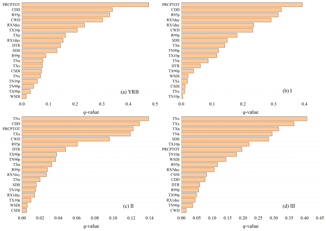
Factor detector analysis quantified the relative explanatory power of each extreme climate index for the spatial variability of modeled NEP using q-values (Figure 9). PRCPTOT had the highest q-value for the entire Yellow River Basin and Zone I, whereas TNx had the highest q-value in Zones II and III. These indices therefore showed the greatest relative explanatory power within their respective spatial units under the specified discretization scheme. CDD had the second-highest q-value for the entire basin and Zones I and II, indicating relatively strong explanatory power for modeled NEP variability in these regions.

3.4.2. Interaction Detector

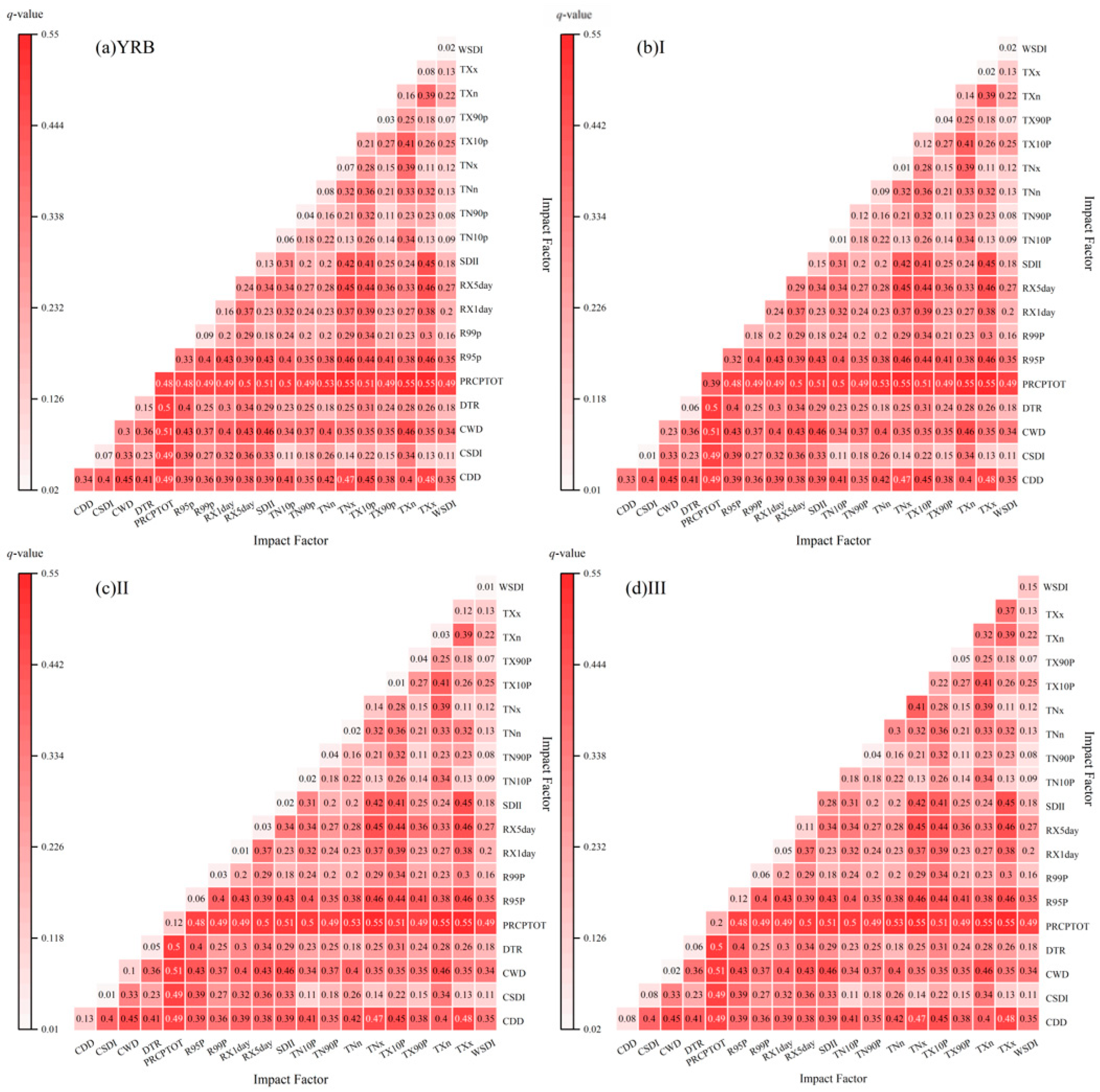
Pairwise interaction detector analysis quantified the joint explanatory power of climatic-factor pairs for modeled NEP variability (Figure 10). Across the analyzed zone–year combinations, no factor pair was classified as independent; the interactions showed either dual-factor enhancement or nonlinear enhancement, relative to the individual q-values. Combinations involving PRCPTOT or R95P frequently yielded relatively high q-values, indicating greater joint explanatory power under the specified discretization scheme.

4. Discussion

4.1. Interpretation of Spatiotemporal Variability in Modeled NEP

Modeled NEP showed an overall increasing tendency across the YRB during 2000–2022, although substantial interannual and spatial variability was also evident. This pattern is consistent with previous reports of vegetation productivity increases associated with ecological restoration and climate variability in parts of the YRB [49,50]. Spatially, the largest modeled NEP increases occurred mainly in the southeastern basin, whereas the northwestern subregion exhibited greater variability. Areas with extremely significant increases, accounting for 49.43% of the basin, formed a broad southwest-to-northeast belt encompassing the Yan–Taihang region, the Qinba Mountains, and the Fenwei Basin transition zone. This spatial correspondence is broadly consistent with the distribution of major revegetation programs, although the present analysis does not isolate their effects from concurrent climatic influences [51]. Localized decreases in parts of Inner Mongolia and central Gansu may be associated with persistent aridity and water limitation [52], while previous studies have also reported vegetation improvements under semi-humid conditions [53]. At the seasonal scale, increasing trends in modeled NEP occurred in all four seasons, with the largest positive trend in summer. Although modeled NEP remained negative in autumn and winter, the values became progressively less negative. The sequential Mann–Kendall analysis of the annual series suggested a possible change in the temporal pattern around 2020, but not a confirmed structural breakpoint. Overall, these patterns should be interpreted as model-derived results conditional on the CASA–Rh framework and its climatic and remote-sensing inputs.

4.2. Climatic Associations with Modeled NEP

Temperature and precipitation are important environmental variables for vegetation productivity and ecosystem respiration [54,55], while extreme events may be associated with abrupt changes in carbon exchange [56]. The present study therefore mapped statistical associations between modeled NEP and extreme-temperature and precipitation indices across the ecological zones of the YRB. At the basin scale, extreme-precipitation indices showed predominantly weak positive correlations with modeled NEP, although significant negative correlations also occurred in some areas. In water-limited arid and semi-arid regions, positive associations may reflect the alleviation of water limitation, whereas the more spatially discontinuous relationships in semi-humid regions may reflect differences in local hydroclimatic conditions. In Zone III, CWD and CDD showed predominantly negative but generally non-significant associations with modeled NEP. The contemporaneous linear analysis cannot identify ecological thresholds or causal mechanisms, and seasonal and lagged responses were not evaluated. Previous studies nevertheless indicate that drought, temperature, and seasonal phenology can jointly affect ecosystem carbon exchange [57,58]. Collectively, the results indicate spatially heterogeneous statistical associations between modeled NEP and extreme-precipitation indices, particularly in water-limited subregions, rather than direct evidence of causal moisture control.

Regarding temperature extremes, most indices examined—including TX10p, TN10p, TX90p, TN90p, TXn, TXx, TNn, and TNx—showed predominantly negative associations with modeled NEP. By contrast, DTR and WSDI exhibited weak positive associations in some areas. These spatial patterns may reflect differences in temperature limitation and growing-season conditions [59], as well as atmospheric water demand and soil moisture availability among ecological zones [60]. However, the present contemporaneous correlation analysis does not directly identify the physiological or ecological mechanisms underlying these relationships. Therefore, the positive and negative associations should be interpreted as statistical covariation rather than as evidence that individual temperature-extreme indices directly enhanced or suppressed ecosystem carbon exchange.

4.3. Limitations and Future Directions

First, the NEP estimates reported in this study are model-derived rather than directly observed. The comparison between CASA-simulated NPP and MOD17A3HGF represents a cross-product consistency assessment, while the comparison of modeled Rh with published regional estimates provides only an order-of-magnitude context. Because basin-wide field or eddy-covariance observations were unavailable, the absolute accuracy of modeled NEP could not be independently validated. Therefore, the reported spatial and seasonal patterns should be interpreted as outputs conditional on the CASA–Rh framework and its remote-sensing and climatic inputs.

Second, the empirical Rh formulation was originally developed under alpine-steppe conditions. Its application to the semi-humid southeastern YRB and its implementation using monthly climatic variables involve spatial and temporal extrapolation, introducing uncertainty into the absolute Rh and NEP estimates. In addition, resampling the approximately 0.1° ERA5-Land fields to a 1 km grid was performed only for spatial alignment and did not increase their effective spatial information. This procedure may smooth local climatic gradients, particularly in the topographically complex Zone III.

Third, the pixel-wise Pearson correlation analysis did not explicitly remove common temporal trends or correct for multiple comparisons. Some extreme climate indices may also exhibit skewed, discrete, or outlier-sensitive distributions. Moreover, the analysis considered contemporaneous annual linear associations only and did not evaluate nonlinear thresholds or lagged climatic effects. Future studies should apply detrending, false-discovery-rate correction, rank-based or permutation methods, and nonlinear or distributed-lag models. The Geodetector results should also be interpreted cautiously because the q-values may depend on the selected discretization method and number of classes [44,45].

Finally, although the quantitative results are specific to the YRB, the ecological-zone-based framework may be applicable to other large river basins with pronounced hydroclimatic gradients. Such applications would require local model recalibration and independent field validation. Complementary time-series remote-sensing indicators, such as dynamic habitat indices [61], could also be incorporated to characterize vegetation productivity, seasonality, and responses to climatic extremes more comprehensively.

5. Conclusions

Integrating satellite remote sensing, reanalysis climate data, and extreme climate indices within a CASA–Geodetector analytical framework, this study characterized the spatial and temporal variability of modeled NEP in the Yellow River Basin during 2000–2022 and examined its statistical associations with extreme-temperature and precipitation indices across three ecological zones. The main conclusions are as follows:

(1)

Basin-wide modeled NEP showed an overall increasing tendency during the 23-year study period, with a Theil–Sen slope of 2.699 g C m⁻² a⁻¹ (p < 0.05). The annual series also exhibited pronounced interannual variability and a possible change in its temporal pattern around 2020. Spatially, increasing trends predominated across the basin and were most extensive in the eastern monsoon-influenced region, whereas the western arid and alpine regions showed greater spatial heterogeneity.

(2)

Modeled NEP increased in all four seasons. Summer exhibited the largest positive trend, while autumn and winter remained characterized by negative modeled NEP values, but became progressively less negative over time. These seasonal patterns represent model-derived estimates and should be interpreted in conjunction with the spatial heterogeneity among ecological zones and the structure of the CASA–Rh framework.

(3)

The direction and strength of the statistical associations between modeled NEP and extreme climate indices differed among ecological zones. Extreme-precipitation indices were generally positively associated with modeled NEP in several water-limited areas, whereas many extreme-temperature indices showed predominantly negative associations. Geodetector results further indicated that precipitation- and temperature-related factors differed in their relative explanatory power among ecological zones, and that pairwise interactions generally exhibited enhanced explanatory power compared with individual factors. These results provide a spatially differentiated, model-based perspective on ecosystem carbon balance in relation to climate extremes across the Yellow River Basin.

References

1. Liu, J.; Wei, L.; Zheng, Z.; Du, J. Vegetation Cover Change and Its Response to Climate Extremes in the Yellow River Basin. Sci. Total Environ. 2023, 905, 167366. [Google Scholar] [CrossRef]
2. Gu, L.; Schumacher, D.L.; Fischer, E.M.; Slater, L.J.; Yin, J.; Sippel, S.; Chen, J.; Liu, P.; Knutti, R. Flash Drought Impacts on Global Ecosystems Amplified by Extreme Heat. Nat. Geosci. 2025, 18, 709–715. [Google Scholar] [CrossRef]
3. Novick, K.A.; Ficklin, D.L.; Stoy, P.C.; Williams, C.A.; Bohrer, G.; Oishi, A.C.; Papuga, S.A.; Blanken, P.D.; Noormets, A.; Sulman, B.N.; et al. The Increasing Importance of Atmospheric Demand for Ecosystem Water and Carbon Fluxes. Nat. Clim. Change 2016, 6, 1023–1027. [Google Scholar] [CrossRef]
4. Tian, H.; Ji, X.; Zhang, F. Spatiotemporal Variations of Vegetation Net Primary Productivity and Its Response to Meteorological Factors Across the Yellow River Basin During the Period 1981–2020. Front. Environ. Sci. 2022, 10, 949564. [Google Scholar] [CrossRef]
5. Wang, J.; Li, L.; Li, Q.; Wang, S.; Liu, X.; Li, Y. The Spatiotemporal Evolution and Prediction of Carbon Storage in the Yellow River Basin Based on the Major Function-Oriented Zone Planning. Sustainability 2022, 14, 7963. [Google Scholar] [CrossRef]
6. Yu, Y.; Hua, T.; Chen, L.; Zhang, Z.; Pereira, P. Divergent Changes in Vegetation Greenness, Productivity, and Rainfall Use Efficiency Are Characteristic of Ecological Restoration Towards High-Quality Development in the Yellow River Basin, China. Engineering 2024, 34, 109–119. [Google Scholar] [CrossRef]
7. Lovett, G.M.; Cole, J.J.; Pace, M.L. Is Net Ecosystem Production Equal to Ecosystem Carbon Accumulation? Ecosystems 2006, 9, 152–155. [Google Scholar] [CrossRef]
8. Chapin, F.S.; Woodwell, G.M.; Randerson, J.T.; Rastetter, E.B.; Lovett, G.M.; Baldocchi, D.D.; Clark, D.A.; Harmon, M.E.; Schimel, D.S.; Valentini, R.; et al. Reconciling Carbon-cycle Concepts, Terminology, and Methods. Ecosystems 2006, 9, 1041–1050. [Google Scholar] [CrossRef]
9. Luan, J.; Ma, N. Responses of Seasonal Hydrological Processes to Vegetation Change in the Yellow River Basin. J. Hydrol. 2025, 660, 133449. [Google Scholar] [CrossRef]
10. Gui, Y.; Wang, K.; Jin, Z.; Wang, H.; Deng, H.; Li, X.; Tian, X.; Wang, T.; Chen, W.; Wang, T.; et al. The Decline in Tropical Land Carbon Sink Drove High Atmospheric CO2; Growth Rate in 2023. Natl. Sci. Rev. 2024, 11, nwae365. [Google Scholar] [CrossRef] [PubMed]
11. Xu, Z.; Liu, D.; Zhao, L.; Wang, J. Sensitivity of Land Carbon Sinks to the Three Major Oscillations in the Northern Hemisphere. Sci. Total Environ. 2024, 955, 177317. [Google Scholar] [CrossRef] [PubMed]
12. Chuai, X.; Qi, X.; Zhang, X.; Li, J.; Yuan, Y.; Guo, X.; Huang, X.; Park, S.; Zhao, R.; Xie, X.; et al. Land Degradation Monitoring Using Terrestrial Ecosystem Carbon Sinks/Sources and Their Response to Climate Change in China. Land Degrad. Dev. 2018, 29, 3489–3502. [Google Scholar] [CrossRef]
13. Zhang, L.; Ren, X.; Wang, J.; He, H.; Wang, S.; Wang, M.; Piao, S.; Yan, H.; Ju, W.; Gu, F.; et al. Interannual Variability of Terrestrial Net Ecosystem Productivity over China: Regional Contributions and Climate Attribution. Environ. Res. Lett. 2019, 14, 014003. [Google Scholar] [CrossRef]
14. Chen, G.; Huang, Y.; Chen, J.; Wang, Y. Spatiotemporal Variation of Vegetation Net Primary Productivity and Its Responses to Climate Change in the Huainan Coal Mining Area. J. Indian Soc. Remote Sens. 2019, 47, 1905–1916. [Google Scholar] [CrossRef]
15. Wang, H.; Wu, L.; Yue, Y.; Jin, Y.; Zhang, B. Impacts of Climate and Land Use Change on Terrestrial Carbon Storage: A Multi-Scenario Case Study in the Yellow River Basin (1992–2050). Sci. Total Environ. 2024, 930, 172557. [Google Scholar] [CrossRef] [PubMed]
16. He, B.; Chen, C.; Lin, S.; Yuan, W.; Chen, H.W.; Chen, D.; Zhang, Y.; Guo, L.; Zhao, X.; Liu, X.; et al. Worldwide Impacts of Atmospheric Vapor Pressure Deficit on the Interannual Variability of Terrestrial Carbon Sinks. Natl. Sci. Rev. 2022, 9, nwab150. [Google Scholar] [CrossRef] [PubMed]
17. He, M.; Kimball, J.S.; Running, S.; Ballantyne, A.; Guan, K.; Huemmrich, F. Satellite Detection of Soil Moisture Related Water Stress Impacts on Ecosystem Productivity Using the MODIS-Based Photochemical Reflectance Index. Remote Sens. Environ. 2016, 186, 173–183. [Google Scholar] [CrossRef]
18. Yuan, W.; Zheng, Y.; Piao, S.; Ciais, P.; Lombardozzi, D.; Wang, Y.; Ryu, Y.; Chen, G.; Dong, W.; Hu, Z.; et al. Increased Atmospheric Vapor Pressure Deficit Reduces Global Vegetation Growth. Sci. Adv. 2019, 5, eaax1396. [Google Scholar] [CrossRef] [PubMed]
19. Alton, P.B.; North, P.R.; Los, S.O. The Impact of Diffuse Sunlight on Canopy Light-use Efficiency, Gross Photosynthetic Product and Net Ecosystem Exchange in Three Forest Biomes. Glob. Change Biol. 2007, 13, 776–787. [Google Scholar] [CrossRef]
20. Gao, M.; Yang, N.; Liu, Q. What Drives Vegetation Evolution in the Middle Reaches of the Yellow River Basin, Climate Change or Human Activities? Sustainability 2024, 16, 10122. [Google Scholar] [CrossRef]
21. Zhong, Z.; He, B.; Wang, Y.-P.; Chen, H.W.; Chen, D.; Fu, Y.H.; Chen, Y.; Guo, L.; Deng, Y.; Huang, L.; et al. Disentangling the Effects of Vapor Pressure Deficit on Northern Terrestrial Vegetation Productivity. Sci. Adv. 2023, 9, eadf3166. [Google Scholar] [CrossRef] [PubMed]
22. Li, X.; Wang, Y.-P.; Lu, X.; Yan, J. Diagnosing the Impacts of Climate Extremes on the Interannual Variations of Carbon Fluxes of a Subtropical Evergreen Mixed Forest. Agric. For. Meteorol. 2021, 307, 108507. [Google Scholar] [CrossRef]
23. Dannenberg, M.P.; Yan, D.; Barnes, M.L.; Smith, W.K.; Johnston, M.R.; Scott, R.L.; Biederman, J.A.; Knowles, J.F.; Wang, X.; Duman, T.; et al. Exceptional Heat and Atmospheric Dryness Amplified Losses of Primary Production during the 2020 U.S. Southwest Hot Drought. Glob. Change Biol. 2022, 28, 4794–4806. [Google Scholar] [CrossRef] [PubMed]
24. Lugato, E. Soil Organic Carbon Losses Exacerbated by Climate Extremes. Nat. Clim. Chang. 2024, 14, 17–18. [Google Scholar] [CrossRef]
25. Zhan, C.; Liang, C.; Zhao, L.; Jiang, S.; Niu, K.; Zhang, Y.; Cheng, L. Vegetation Dynamics and Its Response to Climate Change in the Yellow River Basin, China. Front. Environ. Sci. 2022, 10, 892747. [Google Scholar] [CrossRef]
26. Xu, Y.; Liu, X.; Zhao, L.; Li, H.; Zhu, P.; Liu, R.; Wang, C.; Wang, B. Spatial and Temporal Analysis of Habitat Quality in the Yellow River Basin Based on Land-Use Transition and Its Driving Forces. Land 2025, 14, 759. [Google Scholar] [CrossRef]
27. Cheng, Y.; Chen, Y. Spatial and Temporal Characteristics of Land Use Changes in the Yellow River Basin from 1990 to 2021 and Future Predictions. Land 2024, 13, 1510. [Google Scholar] [CrossRef]
28. Yang, H.; Liu, J.; Li, S.; Mei, S.; Deng, H.; Cheng, F.; Jiang, K.; Liu, T.; Wang, Z. Spatiotemporal Patterns of Habitat Quality and Associated Drivers in Anshun City, China, Based on InVEST and Geodetector. Sci. Rep. 2026. [Google Scholar] [CrossRef] [PubMed]
29. Huang, C.; Sun, C.; Nguyen, M.; Wu, Q.; He, C.; Yang, H.; Tu, P.; Hong, S. Spatio-Temporal Dynamics of Terrestrial Net Ecosystem Productivity in the ASEAN from 2001 to 2020 Based on Remote Sensing and Improved CASA Model. Ecol. Indic. 2023, 154, 110920. [Google Scholar] [CrossRef]
30. Potter, C.S.; Randerson, J.T.; Field, C.B.; Matson, P.A.; Vitousek, P.M.; Mooney, H.A.; Klooster, S.A. Terrestrial Ecosystem Production: A Process Model Based on Global Satellite and Surface Data. Glob. Biogeochem. Cycles 1993, 7, 811–841. [Google Scholar] [CrossRef]
31. Qin, R.; Zhao, Z.; Xu, J.; Ye, J.-S.; Li, F.-M.; Zhang, F. HRLT: A High-Resolution (1d, 1Km) and Long-Term (1961–2019) Gridded Dataset for Surface Temperature and Precipitation across China. Earth Syst. Sci. Data 2022, 14, 4793–4810. [Google Scholar] [CrossRef]
32. Zhao, C.; Wang, C.; Yan, Y.; Shan, P.; Li, J.; Chen, J. Ecological Security Patterns Assessment of Liao River Basin. Sustainability 2018, 10, 2401. [Google Scholar] [CrossRef]
33. Zhu, W.; Pan, Y.; He, H.; Yu, D.; Hu, H. Simulation of Maximum Light Use Efficiency for Some Typical Vegetation Types in China. Chin. Sci. Bull. 2006, 51, 457–463. [Google Scholar] [CrossRef]
34. Pei, Z.-Y.; Ouyang, H.; Zhou, C.-P.; Xu, X.-L. Carbon Balance in an Alpine Steppe in the Qinghai-Tibet Plateau. J. Integr. Plant Biol. 2009, 51, 521–526. [Google Scholar] [CrossRef] [PubMed]
35. Zhang, X.; Liu, C.; Jiang, Y. Spatiotemporal Dynamics of Terrestrial Vegetation Carbon Sinks and Its Response to Climate Change in Northwest China. Front. Environ. Sci. 2025, 13, 1550501. [Google Scholar] [CrossRef]
36. Wang, F.; Cao, Y.; Zhou, S.; Fan, S.; Jiang, X. Estimation of Vegetation Carbon Sink in the Yellow River Basin Ecological Function Area and Analysis of Its Main Meteorological Elements. Acta Ecol. Sin. 2022, 43, 2501–2514. [Google Scholar] [CrossRef]
37. Sen, P.K. Estimates of the Regression Coefficient Based on Kendall’s Tau. J. Am. Stat. Assoc. 1968, 63, 1379–1389. [Google Scholar] [CrossRef]
38. Mann, H.B. Nonparametric Tests Against Trend. Econometrica 1945, 13, 245–259. [Google Scholar] [CrossRef]
39. Kendall, M.G. Rank Correlation Methods, 4th ed.; Charles Griffin: London, UK, 1975. [Google Scholar]
40. Gupta, L.K.; Verma, S. Rainfall and Temperature Trend Analysis Using Mann-Kendall and Sen’s Slope Estimator Test in Kharun Watershed, Chhattisgarh, India. Curr. J. Appl. Sci. Technol. 2023, 42, 1–9. [Google Scholar] [CrossRef]
41. Liu, Z.; Ballantyne, A.P.; Poulter, B.; Anderegg, W.R.L.; Li, W.; Bastos, A.; Ciais, P. Precipitation Thresholds Regulate Net Carbon Exchange at the Continental Scale. Nat. Commun. 2018, 9, 3596. [Google Scholar] [CrossRef] [PubMed]
42. Shi, W.; Zhang, K.; Huang, S.; Huang, Y.; Xie, Y.; Li, Y.; Liu, L.; Forzieri, G. Widespread Declining Sensitivity of Terrestrial Gross Primary Productivity to Compound Dry-Hot Extremes in China. J. Hydrol. 2025, 660, 133387. [Google Scholar] [CrossRef]
43. Luo, W.; Ishii, N.I.; Muraina, T.O.; Song, L.; Te, N.; Griffin-Nolan, R.J.; Slette, I.J.; Ross, S.R.P.J.; Sasaki, T.; Rudgers, J.A.; et al. Extreme Drought Increases the Temporal Variability of Grassland Productivity by Suppressing Dominant Grasses. Ecol. Lett. 2025, 28, e70127. [Google Scholar] [CrossRef] [PubMed]
44. Wang, J.-F.; Li, X.-H.; Christakos, G.; Liao, Y.-L.; Zhang, T.; Gu, X.; Zheng, X.-Y. Geographical Detectors-Based Health Risk Assessment and Its Application in the Neural Tube Defects Study of the Heshun Region, China. Int. J. Geogr. Inf. Sci. 2010, 24, 107–127. [Google Scholar] [CrossRef]
45. Wang, J.-F.; Zhang, T.-L.; Fu, B.-J. A Measure of Spatial Stratified Heterogeneity. Ecol. Indic. 2016, 67, 250–256. [Google Scholar] [CrossRef]
46. Li, Z.-H.; Zhou, D.-M.; Jiang, J.; Ma, J.; Zhu, X.-Y.; Shi, P.; Zhang, J.; Dong, Q.-H. Spatial and Temporal Evolution Characteristics of Carbon Emission from Land Use and Influencing Factors in Gansu Province. Huan Jing Ke Xue Huanjing Kexue 2024, 45, 5040–5048. [Google Scholar] [CrossRef] [PubMed]
47. Bond-Lamberty, B.; Wang, C.; Gower, S.T. A Global Relationship between the Heterotrophic and Autotrophic Components of Soil Respiration? Glob. Change Biol. 2004, 10, 1756–1766. [Google Scholar] [CrossRef]
48. Ma, Y.; Shen, Y.; Jin, L.; Tian, Y.; Ma, H.; Lan, J.; Fu, B. Vegetation-Soil-Microbiota Dynamics across a 50-Year Reconstructed Grassland Chronosequence on the Loess Plateau of China. PeerJ 2024, 12, e18723. [Google Scholar] [CrossRef] [PubMed]
49. Mo, X.; Liu, S.; Hu, S. Co-Evolution of Climate-Vegetation-Hydrology and Its Mechanisms in the Source Region of Yellow River. Acta Geogr. Sin. 2022, 77, 1730–1744. [Google Scholar] [CrossRef]
50. Liu, C.; Wang, P.; Wen, T.; Yu, D.; Bai, W. Spatio-Temporal Characteristics of Climate Change in the Yellow River Source Area from 1960 to 2019. Arid Zone Res. 2021, 38, 293–302. [Google Scholar] [CrossRef]
51. Zhang, M.; Delgado-Baquerizo, M.; Li, G.; Isbell, F.; Wang, Y.; Hautier, Y.; Wang, Y.; Xiao, Y.; Cai, J.; Pan, X.; et al. Experimental Impacts of Grazing on Grassland Biodiversity and Function Are Explained by Aridity. Nat. Commun. 2023, 14, 5040. [Google Scholar] [CrossRef] [PubMed]
52. He, J.; Ju, X.; Han, C.; Liu, L.; Zhang, H.; Adilai, S.; Li, C. Spatiotemporal Dynamics and Driving Mechanism of Eco-Environmental Quality in Piedmont-Oasis-Desert Ecotone Based on Long-Term Harmonized Remote Sensing Ecological Index- Take Korla—Tiemenguan Oasis in Xinjiang as an Example. Environ. Sustain. Indic. 2025, 26, 100611. [Google Scholar] [CrossRef]
53. He, Z.; Guo, Q.; Yin, Z.; Luo, X.; Sun, M. Evolution and Driving Mechanisms of Eco-Environmental Quality across Different Urbanization Stages. Sci. Rep. 2025, 15, 22101. [Google Scholar] [CrossRef] [PubMed]
54. Guo, M.; Zhou, N.; Cai, Y.; Wang, X.; Zhang, X.; Lu, S.; Liu, K.; Zhao, W. Quantitative Estimation of Vegetation Carbon Source/Sink and Its Response to Climate Variability and Anthropogenic Activities in Dongting Lake Wetland, China. Remote Sens. 2025, 17, 2475. [Google Scholar] [CrossRef]
55. Wang, X.; Wang, K.; Zhang, Y.; Gao, J.; Xiong, Y. Impact of Climate on the Carbon Sink Capacity of Ecological Spaces: A Case Study from the Beijing–Tianjin–Hebei Urban Agglomeration. Land 2023, 12, 1619. [Google Scholar] [CrossRef]
56. Wang, Y.; Chen, Y.; Li, Z.; Fang, G.; Wang, C.; Zhang, X.; Li, Y.; Guo, Y. Climatic Factor-Driven Time-Lag Effects of Extreme Precipitation in the Tienshan Mountains of Central Asia. J. Hydrol. 2025, 654, 132902. [Google Scholar] [CrossRef]
57. Piao, S.; Fang, J.; Zhou, L.; Ciais, P.; Zhu, B. Variations in Satellite-Derived Phenology in China’s Temperate Vegetation. Glob. Change Biol. 2006, 12, 672–685. [Google Scholar] [CrossRef]
58. Liu, Q.; Fu, Y.H.; Zeng, Z.; Huang, M.; Li, X.; Piao, S. Temperature, Precipitation, and Insolation Effects on Autumn Vegetation Phenology in Temperate China. Glob. Change Biol. 2016, 22, 644–655. [Google Scholar] [CrossRef] [PubMed]
59. Gan, P.; Liu, F.; Li, R.; Wang, S.; Luo, J. Chloroplasts—Beyond Energy Capture and Carbon Fixation: Tuning of Photosynthesis in Response to Chilling Stress. Int. J. Mol. Sci. 2019, 20, 5046. [Google Scholar] [CrossRef] [PubMed]
60. Sun, W.; Zhou, S.; Yu, B.; Zhang, Y.; Keenan, T.; Fu, B. Soil Moisture-Atmosphere Interactions Drive Terrestrial Carbon-Water Trade-Offs. Commun. Earth Environ. 2025, 6, 169. [Google Scholar] [CrossRef]
61. Safaei, M.; Kleinebecker, T.; Weis, M.; Große-Stoltenberg, A. Tracking Effects of Extreme Drought on Coniferous Forests from Space Using Dynamic Habitat Indices. Heliyon 2024, 10, e27864. [Google Scholar] [CrossRef] [PubMed]
Figure 1. Topographic setting and the three ecological zones used as spatial analytical units in the Yellow River Basin. Roman numerals indicate Zone I (East Asian Monsoon Ecological Zone), Zone II (Western Arid Ecological Zone), and Zone III (Qinghai–Tibet Alpine–Polar Ecological Zone). The base map was prepared using the standard map approved by the Ministry of Natural Resources of China (Approval No. GS (2024) 0650).
Forests 17 00943 g001
Figure 2. Comparison of CASA-simulated NPP with the MOD17A3HGF NPP product across the YRB. (a) Pixel-level relationship between CASA and MODIS NPP; (b) distribution of relative bias (rBias); and (c) distribution of relative root-mean-square error (rRMSE). In panel (a), the color scale indicates the number of observations within each bin; the colors in panels (b,c) are used only for visual distinction.
Forests 17 00943 g002
Figure 3. Basin-wide mean seasonal modeled NEP in the Yellow River Basin during 2001–2022. The values provide an overall temporal summary and do not imply uniform seasonal dynamics across the three ecological zones; the corresponding spatial heterogeneity is shown in Figure 4.
Forests 17 00943 g003
Figure 4. Mean spatial distribution of seasonal modeled NEP across the Yellow River Basin during 2000–2022.
Forests 17 00943 g004
Figure 5. Annual variations and trend diagnostics of modeled NEP in the Yellow River Basin during 2000–2022. (a) Annual NEP values with an overall trend line summarizing the long-term direction of change; the line does not imply a constant rate throughout the study period. (b) Forward (UF) and backward (UB) sequential Mann–Kendall statistics used to examine possible changes in the temporal pattern.
Forests 17 00943 g005
Figure 6. Spatial trends in modeled NEP across the Yellow River Basin during 2000–2022. (a) Theil–Sen slope (β), representing the direction and magnitude of change; (b) combined classification of trend direction and Mann–Kendall significance based on the sign of β and the value of Z. Positive and negative categories indicate increasing and decreasing trends, respectively.
Forests 17 00943 g006
Figure 7. Spatial distribution of pixel-wise Pearson correlation coefficients between modeled NEP and extreme-temperature indices across the Yellow River Basin. Statistical significance was evaluated using the unadjusted pixel-level threshold of p < 0.05. Abbreviations, definitions, and units of the climate indices are provided in Table 2.
Forests 17 00943 g007
Figure 8. Spatial distribution of pixel-wise Pearson correlation coefficients between modeled NEP and extreme-precipitation indices across the Yellow River Basin. Statistical significance was evaluated using the unadjusted pixel-level threshold of p < 0.05. Abbreviations, definitions, and units of the climate indices are provided in Table 2.
Forests 17 00943 g008
Figure 9. Relative explanatory power (q-value) of individual extreme climate indices for the spatial variability of modeled NEP in the Yellow River Basin and its ecological zones. The orange bars represent q-values and are used only for visualization.
Forests 17 00943 g009
Figure 10. Joint explanatory power (q-value) of pairwise interactions among extreme climate indices for modeled NEP in the Yellow River Basin and its ecological zones during 2000–2022.
Forests 17 00943 g010