Article

Effects of Extreme Drought Years on Radial Growth of Oak and Beech on the Swabian Alb, Germany

1
University of Applied Forest Sciences Rottenburg, Schadenweilerhof 1, 72108 Rottenburg, Germany
2
Department of Forestry, University of Applied Sciences Erfurt, Leipziger Straße 77, 99085 Erfurt, Germany
3
Institute of Biology (190a), University of Hohenheim, Garbenstraße 30, 70599 Stuttgart, Germany
4
Department of Geoscience, Physical Geography and Geoinformatics, Eberhard Karls University of Tübingen, Rümelinstraße 19–23, 72070 Tübingen, Germany
*
Author to whom correspondence should be addressed.
Forests 2026, 17(8), 909; https://doi.org/10.3390/f17080909
Submission received: 30 June 2026 / Revised: 28 July 2026 / Accepted: 30 July 2026 / Published: 1 August 2026
(This article belongs to the Section Forest Meteorology and Climate Change)

Abstract

Climate change is increasing drought frequency and severity in Central Europe, with consequences for the productivity and stability of mixed broadleaf forests. We analyzed annual radial growth of European beech (Fagus sylvatica L.) and sessile oak (Quercus petraea (Matt.) Liebl.) along a water-availability gradient on the Swabian Alb (southwestern Germany). At three nearby sites, 45 trees per species were sampled. Tree-ring chronologies were related to meteorological variables and integrated drought indices (PDSI/scPDSI, SMI). Extreme dry and wet years were identified from detrended growing-season indices, and event responses were quantified using resistance, recovery, and resilience metrics and their humid-year analogues. Annual growth variation was primarily site-driven rather than species-driven, highlighting strong control by local soil water availability. Correlation analyses showed that integrated drought and soil-moisture indices explained radial growth more consistently than single climate variables. Oak showed higher drought resistance than beech in several events, although the magnitude and significance of this difference depended on site and drought year. Resistance generally declined toward recent events, particularly at Site 2, while recovery tended to increase. Recovery did not consistently favor either species, and resilience remained broadly stable, except for a decline in beech during the most recent drought events. Overall, sensitivity to drought is jointly controlled by species identity and fine-scale site conditions: oak has a comparatively robust resistance advantage, whereas post-drought recovery and resilience are strongly context-dependent. These findings support site-specific species mixtures and silvicultural strategies to sustain forest function under increasing drought risk.

1. Introduction

Recent sequences of consecutive warm and dry years increasingly affected forest growth across Central and Western Europe, with substantial ecological and economic consequences [1,2,3]. Drought is now recognized as a major driver of reduced radial stem growth, declining vitality, and elevated mortality risk for many temperate tree species [4,5,6,7]. However, drought impacts are rarely determined by climate alone. They are strongly modulated by local water availability, soil depth, rooting conditions, and stand structure. Therefore, tree-growth responses must be interpreted using both regional climate signals and site-specific indicators of soil moisture and water limitation [8,9].
European beech (Fagus sylvatica L.) and sessile oak (Quercus petraea (Matt.) Liebl.) are particularly relevant in this context. Both species are key components of Central European broadleaf forests and are widely present in mixed stands [10,11,12,13,14]. Current silvicultural guidelines promote mixed broadleaf stands as part of climate-change induced drought adaptation strategies [15,16]. Yet the future role of beech in such mixtures remains uncertain because recent studies report pronounced drought-related reductions in growth and vitality, whereas oak shows comparatively higher drought tolerance [17,18,19,20,21,22,23,24]. It remains unclear whether these species differences are consistent across local water-availability gradients or whether site conditions can amplify, weaken, or even override species-specific drought responses.
The Swabian Alb, a mountain range in southwestern Germany, provides a suitable setting to address this question. Its shallow, calcareous, and partly skeletal soils can generate strong small-scale contrasts in plant-available water [25]. Such heterogeneity allows oak and beech responses to be compared along a dry-to-moist gradient while minimizing broad-scale climatic differences. Tree-ring analysis is especially useful for this purpose because it provides annually resolved growth records and enables retrospective assessment of tree responses before, during, and after extreme years [26].
A challenge is the definition of drought. Single meteorological variables such as precipitation or temperature may not capture the cumulative water deficits that are most relevant for tree growth. Integrated indicators can provide a more biologically meaningful representation of drought stress. The Palmer Drought Severity Index (PDSI) and its self-calibrated form (scPDSI) combine precipitation and atmospheric evaporative demand to estimate cumulative moisture deficits and support comparisons across years and regions [27,28,29,30]. The Soil Moisture Index (SMI) complements these climate-based indicators by representing water availability in the soil profile and thus linking meteorological drought more directly to potential rooting-zone stress [31]. Combining these indicators with tree-ring data enables a more robust assessment of hydroclimatic extremes and their translation into growth resistance, recovery, and resilience.
This study investigates annual radial growth dynamics of sessile oak and European beech at three nearby sites in the Swabian Alb that differ in local soil water availability. We combine chronology statistics, climate-growth correlations, pointer-year analyses, and event-based response metrics to identify drought-vulnerability patterns and derive site-specific implications for the management of drought-prone mixed broadleaf forests.
The specific objectives are:
  • to identify extreme dry and wet years using climatic and soil-moisture indicators;
  • to quantify interannual growth variability and common growth signals within and between species and sites;
  • to determine which climatic and drought-related variables most strongly control radial growth;
  • to assess drought response components, particularly resistance, recovery, and resilience, in oak and beech;
  • to derive practical recommendations for species selection and stand development under increasing drought risk in southwestern Germany.
Based on previous evidence and regional drought development, we test the following hypotheses:
H1. 
Climate-growth relationships are stronger for integrated drought indicators (PDSI/scPDSI and SMI) than for single meteorological variables.
H2. 
Beech shows stronger growth reductions and lower drought resistance than oak during extreme dry years.
H3. 
Species differences in drought response increase with decreasing site water availability.
H4. 
Recovery and resilience after drought differ between species and site conditions, indicating contrasting adaptation potential under future drought-prone forest conditions.

2. Materials and Methods

2.1. Study Site and Tree Selection

The study was conducted at three sites in a mixed temperate forest northeast of Hechingen (Baden-Württemberg, Germany). Mean annual temperature is 9.2 °C for 1991–2020, which is 1.0 °C higher than for 1961–1990; mean annual precipitation is 806 mm, 8 mm lower than for 1961–1990, with approximately one-third falling between May and July. The sites were selected to ensure close co-occurrence of sessile oak (Quercus petraea) and European beech (Fagus sylvatica) under contrasting local soil water regimes. Although geographically close, the sites differ in topographic position and elevation, resulting in distinct micro-environmental conditions. Site 1 is located on a gentle northwest-facing slope (5°) at 520 m a.s.l., Site 2 on a steeper southwest-facing slope (15–20°) at 550 m a.s.l., and Site 3 near a steep escarpment at 850 m a.s.l. (Table 1). All soils developed from the Middle Jurassic Opalinuston Formation as parent material but differed in depth and physical structure: Sites 1 and 2 are clay-rich marl-derived soils (Vertic Cambisol and Haplic Vertisol, respectively), whereas Site 3 is a shallow, stony limestone soil (Rendzic Leptosol). Although soil drainage was not measured directly, these site characteristics imply contrasting water balances. At Site 1, the gentle northwest-facing slope and relatively deep, clay-rich soil likely reduce surface runoff and lateral drainage while increasing soil-water storage. At Site 2, the steeper southwest-facing slope likely enhances runoff and downslope drainage and receives greater solar exposure, which may increase evaporative demand despite the clay-rich soil. At Site 3, the shallow, stony soil has a low water-storage capacity, and its position near the escarpment may facilitate rapid drainage, reducing the amount of water available to roots between precipitation events. Phosphorus availability may be constrained by elevated calcium content at Site 3. The Hechingen station (approximately 518 m a.s.l.) is representative of Sites 1 and 2 and averages 39 snow-cover days and a frost-free period of 174 days per year (1991–2020). In contrast, the higher-elevation Trochtelfingen station (approximately 800 m a.s.l.), which is more representative of Site 3, averages 63 snow-cover days and a shorter frost-free period of 155 days. Site 3 therefore likely experiences a longer freezing season and more persistent snow cover than Sites 1 and 2 [32]. All sites belong to the “DryTrees” monitoring framework and are described in detail by Mauz et al. [33], which also includes a map showing the location of the Swabian Alb and a satellite map of the sites. Immersive 360° panoramas of the locations are available at https://36o.de/drytrees/ (accessed on 29 July 2026) [34].
At each site, 15 oak and 15 beech trees were selected within 0.2–0.45 ha, yielding a total of 45 individuals per species. Stand structure varied markedly among sites: Site 1 had the lowest basal area and stem density but larger mean tree dimensions, whereas Sites 2 and 3 were denser and characterized by smaller tree sizes (stem DBH ≥ 7 cm). Mean tree age was approximately 100 years at Sites 1 and 2, whereas trees at Site 3 were substantially older, with several individuals approaching 200 years. Tree ages were estimated from increment cores taken from all sampled trees (see Section 2.3). Reported minimum ages likely underestimate true establishment ages because many cores did not reach the pith and sampling was conducted at breast height and not at the stem base. Species composition at all sites was beech-dominated (56%–78%), while oak accounted for 8%–21% of stems; hornbeam (Carpinus betulus) and ash (Fraxinus excelsior) occurred locally.

2.2. Climate Data and Indices

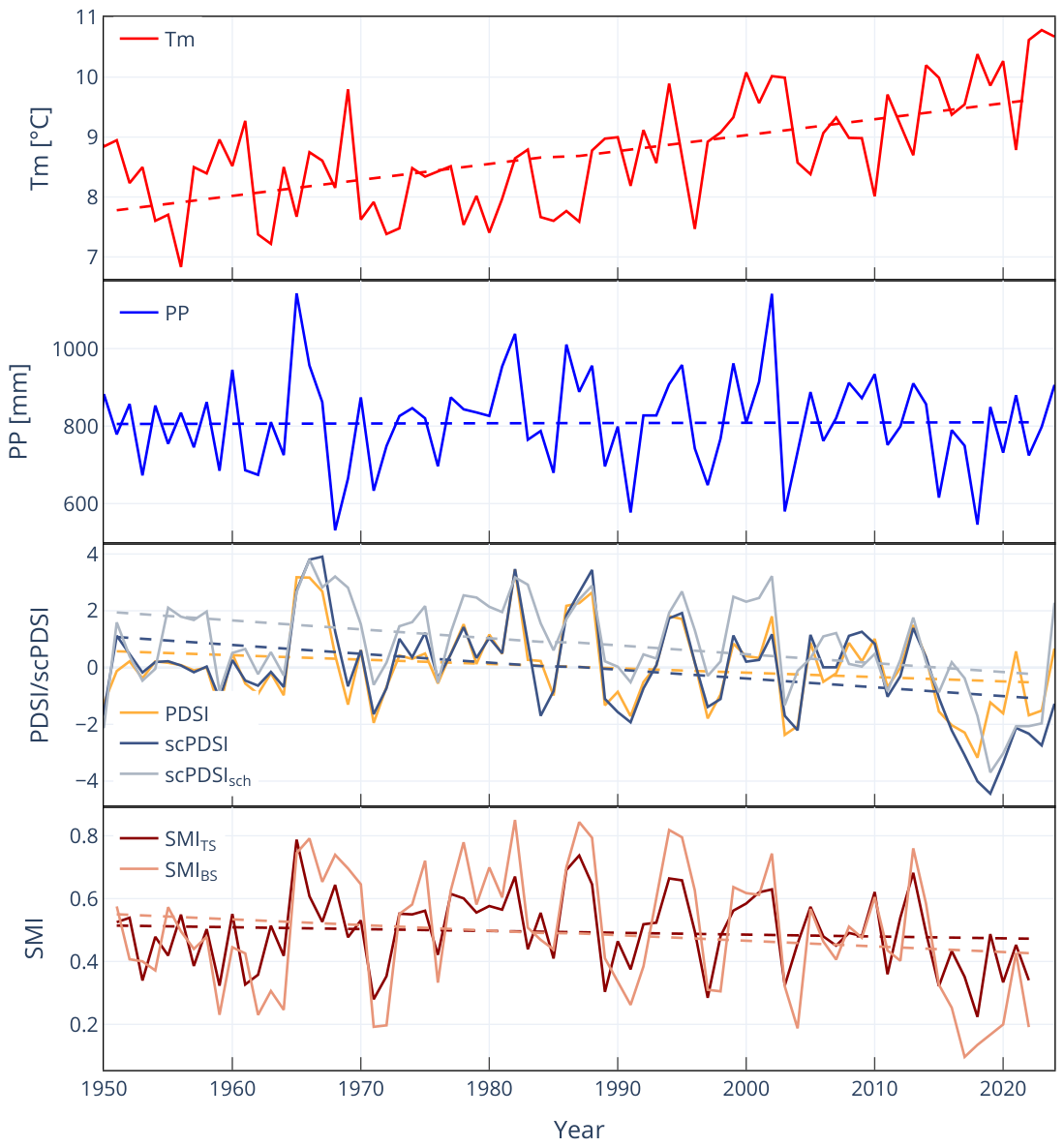
Meteorological data for 1947–2024 were obtained from the German Weather Service (Deutscher Wetterdienst, DWD) station Hechingen (station ID 2074; ~520 m a.s.l.; [32]). Daily temperature and precipitation records were aggregated to monthly and annual time series (Figure 1) for drought-index calculations and climate-growth analyses. Because the three forest sites are close to one another, the station data provide a consistent regional climate signal; however, precipitation at Site 3 may be underestimated because of topographic effects near the escarpment.
Drought intensity was quantified using the Palmer Drought Severity Index (PDSI; [27]) and the self-calibrated PDSI (scPDSI; [28]), both of which range from −4 (extreme drought) to +4 (very wet). Compared with single meteorological variables, these indices integrate water supply and atmospheric demand and are therefore well suited for characterizing cumulative moisture deficits relevant to tree growth [30,35]. Potential evapotranspiration (PET) was calculated with the Python package pyet 1.4 [36] following Oudin [37], using daily mean temperature and latitude. Monthly PET and precipitation were then used to compute PDSI and scPDSI with the R package scPDSI. For cross-checking and broader spatial comparability, we additionally used gridded scPDSI products from Van Der Schrier et al. [29] and Dunn et al. [38] (hereafter scPDSI s c h ; Figure 1).
Figure 1. Annual mean air temperature (Tm), precipitation totals (PP), and annual averages for the PDSI, the scPDSI (including global gridded data from Van Der Schrier et al. [29] and Dunn et al. [38], scPDSI s c h ), as well as the topsoil soil moisture index ( SMI T S ) and the bulk-soil moisture index ( SMI B S ). The colored dashed lines represent the respective linear trend. The data span from 1950 to 2024 (1951 to 2022 for SMI) and refer to the weather station in Hechingen, ~520 m a.s.l.
Forests 17 00909 g001
To complement climate-based indices, we extracted Soil Moisture Index (SMI) data for the period 1951–2022 from the German Drought Monitor [31]. This product is available at 4 × 4 km spatial resolution and provides estimates for topsoil moisture ( SMI T S , upper 25 cm) and bulk soil moisture ( SMI B S ; Figure 1). Including SMI enables a more direct link between meteorological drought and site-level water availability in the rooting zone. Sites 1 and 2 were located within the same 4 × 4 km model grid cell, whereas Site 3 fell within an adjacent grid cell. Accordingly, climate-growth correlation analyses for Site 3 were based on climate data extracted from its respective grid cell. However, the climate time series of the two grid cells were highly similar, with Pearson correlation coefficients of 0.99 and 0.91 for SMI T S and SMI B S , respectively. For clarity, Figure 1 presents only the SMI time series for the grid cell containing Sites 1 and 2. Intercorrelations among all climate variables and drought indices used in this study are provided in Table 2. As with precipitation, uncertainty may be somewhat higher at Site 3 because shallow, stony soils and local topographic effects are not fully represented by the gridded product.

2.3. Tree-Ring Data

For each tree, two increment cores (5 mm diameter) were extracted at breast height (1.30 m) from opposite directions perpendicular to the slope, using increment borers (Haglöf Sweden AB, Långsele, Sweden). This design was chosen to reduce within-tree variability and strengthen cross-dating reliability. Cores were mounted on wooden supports and surface-prepared with a core microtome to obtain clear annual-ring boundaries [39]. Ring widths were measured using WinDENDRO 2019 (Regent Instruments Inc., Quebec City, QC, Canada). Cross-dating quality and measurement plausibility were checked using xDateR (https://viz.datascience.arizona.edu/xDateR/ (accessed on 29 July 2026)). Cores were retained when 30-year segments reached a minimum correlation of 0.30 with the respective master chronology. If this criterion was met only for part of a core, only the reliable segment was retained. When one core of a tree was not usable, the second core was used alone. Final sample depth and retained series are reported in Table A1. For tree-level series construction, the two core measurements per tree were combined using the root mean square (RMS). Raw ring-width series were retained for analyses of growth-response metrics (resistance, recovery, and resilience), whereas detrended series were used for chronology statistics and climate-growth analyses.
To remove age- and size-related trends, ring-width series were detrended in two steps: first with a linear function and then with a spline using a 50% frequency cut-off at 30 years. Detrending was performed with dplPy ([40], dplpy Version 0.1.5), a Python implementation inspired by dplR workflows [41]. Site- and species-specific chronologies (RWI = Ring Width Index) were built from standardized tree-ring series after prewhitening to reduce residual autocorrelation. Variance-stabilized chronologies were generated with a minimum moving-window length of 30 years.
Chronology quality and pointer years were calculated using the interval trend (Gleichläufigkeit) following Schweingruber [42,43]. Years with an interval trend greater than 75% were considered pointer years and were compared with extreme years identified from the drought indices.

2.4. Identification of Extreme Years

Extreme dry and wet years were identified using growing-season (April–September) mean values of scPDSI for 1950–2024 and SMI B S for 1951–2022. To reduce bias caused by pronounced recent trends, especially during the last decade (Figure 1), both index series were linearly detrended before threshold classification.
Growing seasons were classified as extreme dry years when detrended scPDSI or detrended SMI B S values fell below the 5th percentile, and as extreme wet years when values exceeded the 95th percentile. Consecutive extreme years were grouped and treated as a single extreme event (Table 3).

2.5. Calculation of Growth-Response Metrics

Growth responses to hydroclimatic extremes were quantified using resistance ( R t ), recovery ( R c ), and resilience ( R s ) following Lloret et al. [26]. These indices characterize the magnitude of growth reduction during stress events and subsequent post-event recovery of radial stem growth. All calculations were based on individual-tree ring-width series.
R t = EY / PreEY
R c = PostEY / EY
R s = PostEY / PreEY
Here, EY denotes tree-ring width during the event year (or mean tree-ring width during multi-year events), PreEY denotes mean tree-ring width over the 5-year period preceding the event, and PostEY denotes mean tree-ring width over the 5-year period following the event.
In addition, we estimated growth recovery time (GRT) and increment loss due to drought (Loss) following Thurm et al. [44]. GRT indicates the number of years required for annual growth to return to pre-drought levels, and Loss quantifies the cumulative difference between observed growth and the pre-drought reference during that period. Loss was retained as a signed metric: negative values indicate growth below the pre-drought reference, with more negative values representing greater cumulative growth loss, whereas positive values indicate growth above the reference. The maximum GRT was set to 10 years, although no observed recovery time reached this cap. GRT was treated as missing when event-period growth exceeded pre-drought growth because no event-related growth reduction occurred. For the 2017–2019 event, GRT was also set to missing when recovery had not occurred by the end of the available series in 2024.
We also calculated average growth reduction (AGR) and average recovery rate (ARR; [21]). AGR was calculated as Loss divided by GRT and retained the sign of Loss; negative AGR values therefore indicate an average annual growth deficit relative to the pre-drought reference. ARR was calculated as 1 R t / GRT , multiplied by 100, and reported as a percentage. Negative ARR values occur when R t > 1, indicating that event-period growth exceeded pre-drought growth and that no event-related growth reduction occurred. AGR quantifies the mean annual impact of drought, whereas ARR reflects the proportion of the event-period growth reduction recovered per year.
Resistance ( R t ), recovery ( R c ), and resilience ( R s ) were also determined for extreme wet years using analogous event-year, pre-event, and post-event growth windows. In contrast to drought conditions, wet years are generally not expected to cause growth reductions. Nevertheless, we retained the established terminology to maintain consistency, while acknowledging that the ecological meaning of these metrics differs between dry and wet extremes. These results are provided in Appendix B Figure A1 and Figure A2.

2.6. Statistical Analysis

Relationships between tree growth and climate variables were assessed using Pearson’s correlation coefficient. Correlations were calculated between detrended tree-ring chronologies for each species and site and monthly, growing-season, or annual climate variables. Statistical significance was evaluated at p < 0.05. Differences in tree growth responses between species and among sites were examined separately for each drought event. Because the response variables did not consistently satisfy the assumptions of parametric analysis of variance, aligned rank transform (ART) factorial analyses of variance were used [45]. A separate model was fitted for each response variable and drought event, with species, site, and the species × site interaction included as fixed effects. Significant interactions were followed by ART-C simple-effects contrasts. Species were compared within each site, with Holm adjustment across the three sites, whereas sites were compared pairwise within each species, with Holm adjustment applied separately for oak and beech. When the interaction was not significant, significant marginal effects of species and site were interpreted, and pairwise site comparisons were Holm-adjusted. Results are reported as medians and interquartile ranges. Aligned rank transform (ART) omnibus results for site, species, and their interaction, including Benjamini–Hochberg-adjusted p-values across events, are provided in Appendix A Table A2. To assess the temporal development of growth responses around drought events, average growth deviations were calculated for the drought year and for the five years preceding and following each event. Growth deviations were expressed relative to the mean tree-ring width of the five years preceding the drought event, which served as the reference period. Uncertainty around mean growth deviations was quantified using 90% bootstrap confidence intervals based on 9999 bootstrap iterations. Confidence intervals were derived separately for each species and site and were used to illustrate the variability and robustness of observed growth responses. Exploratory temporal trends across the four event periods were assessed using linear regressions of site-level median response metrics against event year, separately for each species and site. Because only four event periods were available, these trends were interpreted descriptively; line intensity in the trend figures reflects the statistical significance of the fitted slopes. Aligned rank transform factorial analyses and ART-C contrasts were conducted in R using the ARTool package 0.11.2 [46]. All remaining statistical analyses were conducted in Python 3.10.13 using pandas 2.3.3 [47], NumPy 1.24.0 [48], and SciPy 1.15.3 [49]. Data visualization and figure generation were performed using Plotly 5.22.0 [50].

3. Results

3.1. Tree-Ring Chronologies

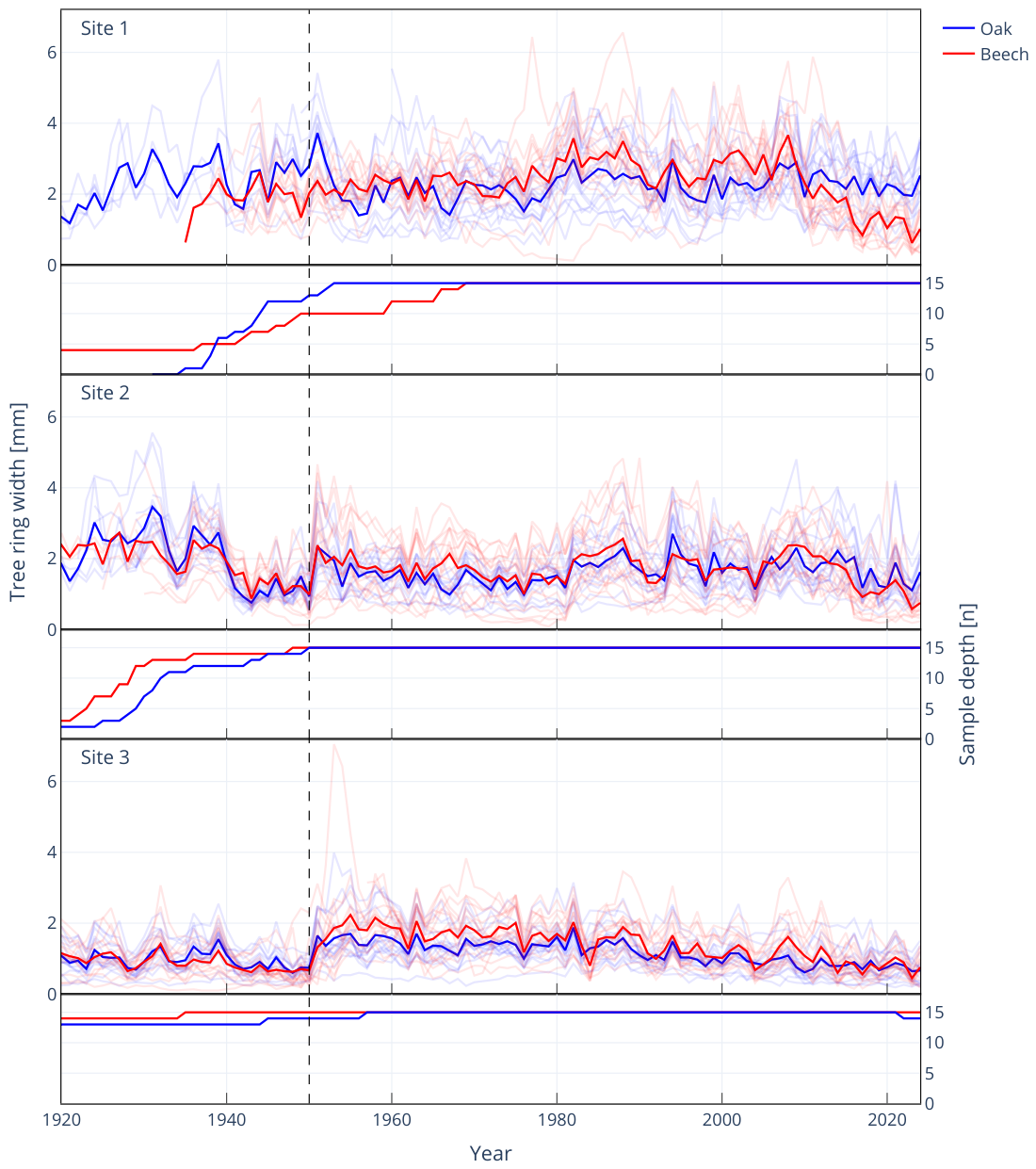
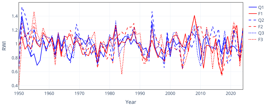
Across all sites, individual tree-ring series showed pronounced interannual variability, while site-level mean chronologies displayed coherent common signals (Figure 2). A marked increase in ring width occurred around 1950 (vertical dashed line in Figure 2), most clearly at Sites 2 and 3. Thereafter, growth trajectories diverged among sites: Site 3 showed a long-term decline from approximately 1960 onward in both species, whereas Sites 1 and 2 remained comparatively stable through much of the late twentieth century. Mean annual ring width was highest at Site 1 (oak/beech: 2.30 ± 0.47/2.29 ± 0.34 mm), intermediate at Site 2 (1.73 ± 0.30/1.71 ± 0.40 mm), and lowest at Site 3 (1.09 ± 0.18/1.19 ± 0.21 mm). Differences in stand structure provide relevant context for these patterns. Trees at Site 3 were substantially older (oak/beech: 168.2 ± 30.0/149.4 ± 34.1 years) than trees at Site 1 (104.2 ± 38.7/87.0 ± 3.9 years) and Site 2 (111.9 ± 25.1/101.1 ± 6.4 years), and also had narrower and less variable rings (Table 1). Overall, temporal variability in annual radial growth was similar for both species, although pronounced interspecific differences occurred in 1966 and 1967 at Sites 1 and 2, when oak growth was substantially lower than beech growth. From 2008 onward, radial growth declined across all sites, with the strongest reductions at Site 2 for both species and at Site 1 for beech. In contrast, oak at Site 1 and both species at Site 3 showed weaker recent declines (Figure 2). Detrended tree-ring chronologies for both species across the three study sites were free of long-term growth trends and confirmed these between-site contrasts and species-specific synchronicity (Figure 3). Intercorrelation analysis (Table 4) showed strong positive correlations among all site chronologies. For oak, the correlation was highest between Sites 1 and 2 (0.61), followed by Sites 2 and 3 (0.57) and Sites 1 and 3 (0.52). Beech correlations varied little among site pairs (0.54–0.56). Within-site oak-beech correlations were stronger at Sites 2 and 3 than at Site 1.

3.2. Impact of Climate on Growth

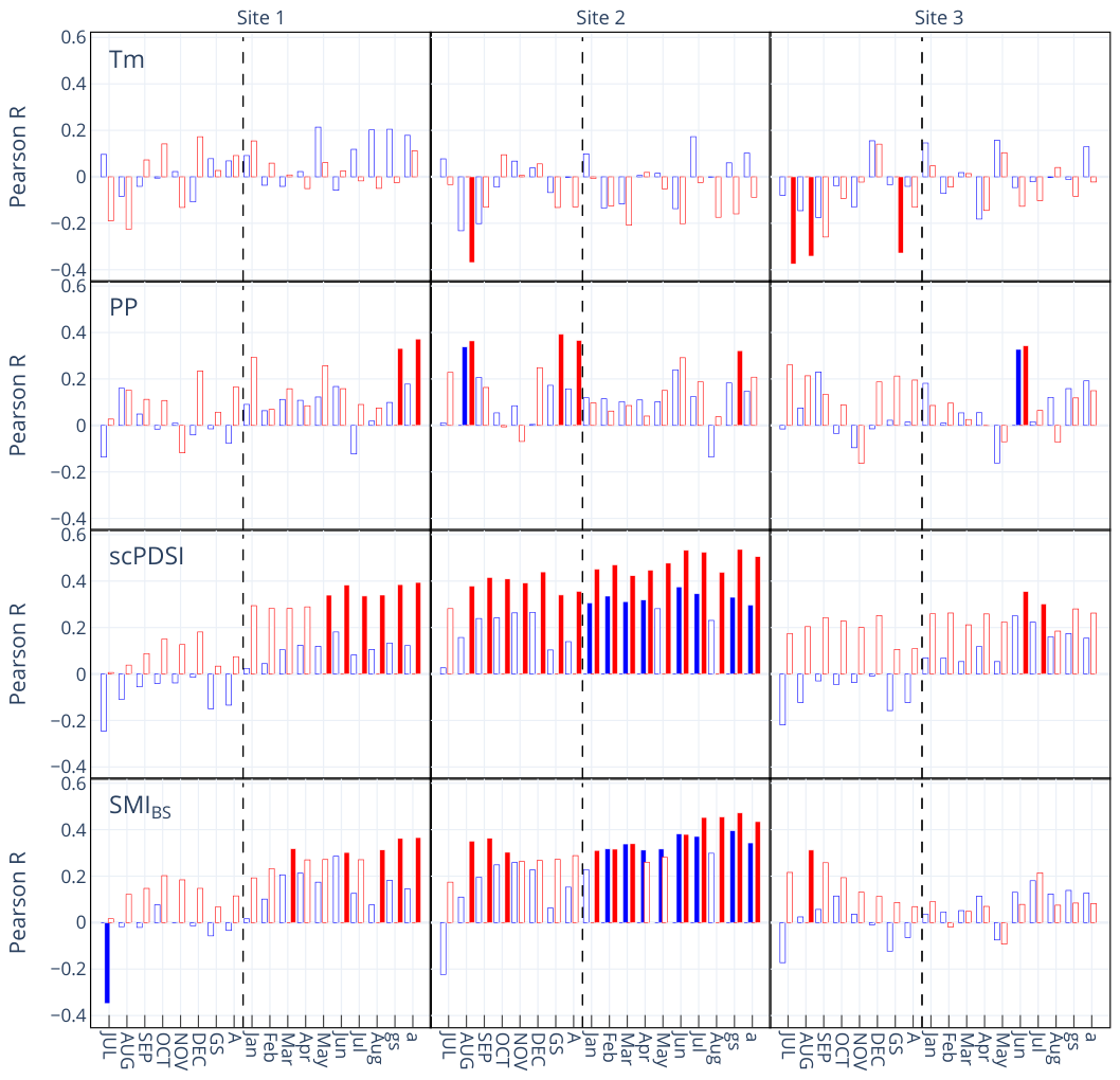
Climate-growth correlations were analyzed to identify the seasonal windows and hydroclimatic variables most strongly associated with radial growth of beech and oak at each site (Figure 4). Correlations were computed from July of the previous year to August of the current year and for aggregated periods, including the previous and current growing seasons and the previous and current full years. Across sites and species, integrated drought indicators (scPDSI and SMI B S ) showed clearer and more frequent significant relationships with annual radial growth than single meteorological variables (precipitation and temperature). In general, correlations with current-year growing-season hydroclimatic conditions were stronger than correlations with previous-year conditions, indicating that growth was primarily controlled by moisture availability during the current vegetation period. Species-specific differences were consistent along the site gradient: beech generally exhibited stronger climate sensitivity than oak, particularly at Site 2. At this intermediate site, both species tracked variability in scPDSI and SMI B S most closely, with multiple significant correlations in growing-season windows. At Site 1, strong relationships were more pronounced for beech than for oak, whereas at Site 3, correlations were present but overall weaker and more variable among months. For precipitation alone, significant correlations were less consistent and mostly site-specific. Temperature showed predominantly negative relationships with growth in July and August of the previous year, especially at Site 3, suggesting enhanced growth limitation under warm conditions when water availability was low. Annual radial growth of oak was consistently negatively correlated with SMI B S in July of the previous year, with a statistically significant relationship at Site 1.

3.3. Growth Responses to Extreme Years

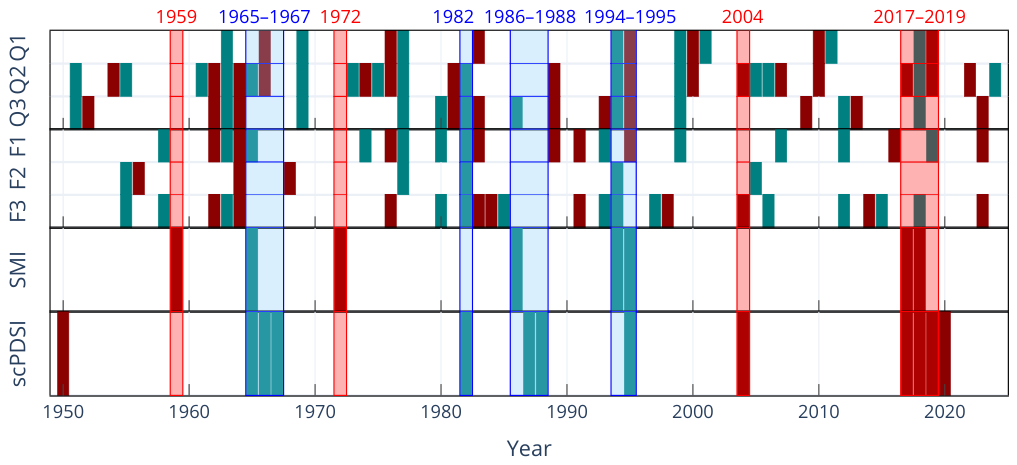
Pointer years were irregularly distributed from 1950 to 2024 and showed no clear long-term trend (Figure 5). Major negative pointer years, detected in at least three of the six site- and species-specific chronologies, occurred in 1962, 1964, 1976, 1983, 1989, 1995, and 2023. Positive pointer years frequently followed negative pointer years, indicating renewed growth after strongly reduced increments. Conversely, the negative pointer years in 1964, 1983, and 1995 followed positive pointer years and may therefore partly represent relative growth declines after exceptionally wide rings.
Correspondence between pointer years and hydroclimatic extremes was event-specific. The extremely dry edaphic conditions in 1959 and 1972 were not associated with negative pointer years. In contrast, the 2004 drought coincided with negative pointer years for oak at Site 2 and beech at Site 3, while the 2017–2019 drought was reflected only in oak at Sites 1 and 2. Exceptionally wet periods, which were generally consistent between SMI and scPDSI, were often associated with positive pointer years, particularly at their onset and largely irrespective of site or species.
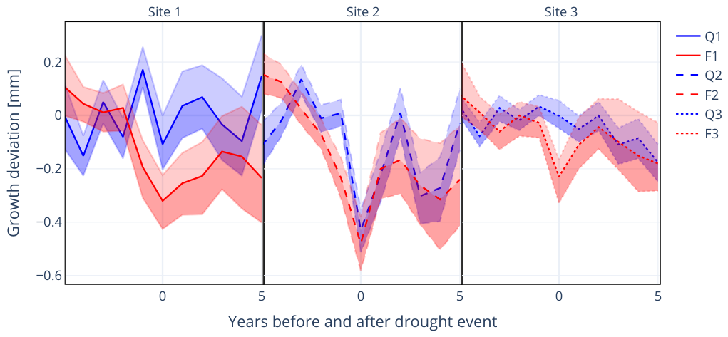
Average growth deviations during the five years before and after drought events showed that beech generally responded with stronger growth reductions than oak across the three sites (Figure 6). At Site 2, the magnitude of the growth reduction was comparable between oak and beech. In contrast, oaks at Site 3 did not exhibit an immediate growth reduction during the drought event; however, a pronounced decline in radial growth became apparent over the subsequent five years. Similarly, at Site 2, a strong growth reduction occurred during the five years following the drought event. Although both species initially showed signs of recovery during the first two post-drought years, this was followed by a marked decline in growth.
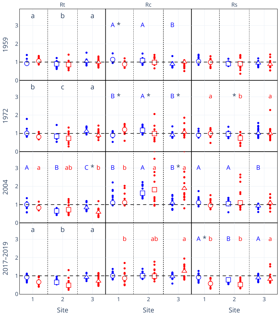
Resistance, recovery, and resilience exhibited substantial variability among drought events and study sites (Figure 7). Resistance ( R t ) was lower at S2 than at S1 and S3 in 1959. In 1972, oak was more resistant than beech across sites, and resistance followed the order S3 > S1 > S2. A significant species × site interaction occurred in 2004 ( F 2 , 84 = 7.08, p = 0.001): oak was more resistant than beech at S3, resistance was lowest at S2 within oak, and lower at S3 than at S1 within beech (all p Holm < 0.001). In 2017–2019, oak was again more resistant than beech, while resistance at S2 was lower than at S1 and S3 (all p Holm < 0.001).
Recovery ( R c ) showed significant species × site interactions in all drought events (all p ≤ 0.029). Oak recovered more strongly than beech at S1 in 1959. In 1972, beech recovery exceeded that of oak at S1 and S3, whereas oak recovered more strongly at S2. In 2004, recovery was highest at S2 and S3 in beech and at S2 in oak; beech also recovered more strongly than oak at S3. In 2017–2019, the only significant follow-up difference was greater beech recovery at S3 than at S1.
Resilience ( R s ) differed among sites in 1959 (p = 0.035), although no pairwise contrast remained significant after Holm adjustment. Significant species × site interactions occurred in 1972, 2004, and 2017–2019 (all p ≤ 0.024). In 1972, beech resilience was lower at S2 than at S1 and S3 and lower than oak resilience at S2. In 2004, oak resilience was lower at S3 than at S1 and S2, without significant species differences. In 2017–2019, beech resilience was highest at S3, oak resilience was lowest at S2, and oak was more resilient than beech at S1.
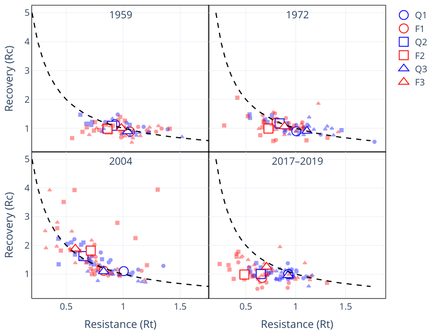
Together, Figure 7 and Figure 8 show that lower drought resistance was often offset by stronger recovery. Consequently, many tree-level observations and site medians remained close to the resilience-1 curve in 1959, 1972, and 2004 despite significant species and site effects. This compensation weakened during 2017–2019, when low resistance coincided with low recovery, most clearly for beech at Site 2.
GRT and Loss differed most clearly in 1972 (Table 5). Beech had a longer GRT than oak at S1 and S2, and beech GRT was longer at these sites than at S3 ( F 2 , 79 = 10.17, p < 0.001; all p Holm ≤ 0.014). In 2004, GRT was longer at S3 than at S1 and S2 (both p Holm ≤ 0.001). The 1972 interaction for Loss ( F 2 , 79 = 5.22, p = 0.007) reflected more negative values for beech than oak at S1 and more negative beech Loss at S1 and S2 than at S3 (all p Holm ≤ 0.049). In 2017–2019, Loss was more negative at S2 than at S3 ( p Holm = 0.014).
AGR was higher in oak than beech and lower at S2 than at S3 in both 1972 and 2017–2019 (p = 0.009; p Holm ≤ 0.011). In 2004, oak AGR was lower at S2 than at S1 and S3 ( F 2 , 77 = 3.18, p = 0.047; both p Holm = 0.004). ARR showed species × site interactions in 1959, 1972, and 2004 (all p ≤ 0.037): beech was lower than oak at S1 in 1959, higher at S3 in 1972, and lower at S2 in 2004 (all p Holm ≤ 0.020). Oak ARR followed S2 > S1 > S3 in 1972 and was highest at S2 in 2004; ARR was also higher at S2 than at S1 and S3 in 2017–2019 (both p Holm = 0.041).
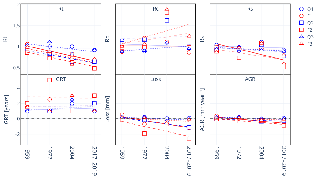
Contrasting temporal trajectories for R t , R c , and R s across drought years are shown in Figure 9. Resistance ( R t ) generally declines from 1959 toward recent events, with the strongest negative trends at Site 2 for both species (dashed lines) and at Site 1 for beech (red solid line); Site 3 shows weaker and less consistent declines. Recovery ( R c ) exhibits the opposite pattern, with increasing values over time at most sites and the steepest positive trends for beech at Sites 2 and 3 (red dashed and dotted lines). Oak also shows increasing R c , but generally with lower slopes than beech. In contrast, resilience ( R s ) remained comparatively stable around the reference level ( R s = 1), with a slight negative trend for beech at Site 1 (red solid line), whereas beech at Site 3 showed a positive tendency and reached the highest late-period R s values. Overall, the data indicate a shift from higher resistance in earlier drought years toward lower resistance but stronger post-drought recovery in recent drought years, especially for beech. GRT increased slightly from the 1959 drought event to the 2017–2019 event. For beech at Sites 1 and 2, significant trends indicated increasing growth losses (lower Loss values) and stronger average growth reductions (lower AGR values).

4. Discussion

4.1. Long-Term Growth Patterns and Site Controls

Radial tree stem growth increased sharply after 1945 (Figure 2), particularly at Sites 2 and 3, whereas the increase at Site 1 was less pronounced. This abrupt rise is most likely related to post-war stand thinning than to climate effects, given the severe timber shortage in post-war Germany [51]. Since then, growth at Site 3 has declined steadily, probably reflecting the combined effects of increasing tree age and competition for water on the shallow, rocky soils.
Since 2008, growth has declined strongly across all sites, with the most pronounced reductions in beech (Figure 2). This contrasts with recent observations from Czechia, where most beech and oak trees showed no growth decline. Kašpar et al. [52] reported that negative growth trends in beech were mainly associated with lower elevations, whereas individuals at higher elevations were more likely to show positive trends. The strongest positive trend occurred at approximately 800 m, which is close to the elevation of Site 3. Likewise, approximately 80% of oaks showed positive growth trends, with a slightly stronger tendency at higher elevations. The recent decline observed in our study therefore suggests that local edaphic and stand conditions can override elevation-related expectations.
Overall, growth rates were highest at Site 1 and lowest at Site 3. Site 1 is located at lower foothill elevations and probably offers better water availability than the other sites. This interpretation is consistent with the view that drought impacts in temperate forests are strongly modulated by site-specific water availability [53] and rooting-zone constraints, even under a shared regional climate signal. In contrast, Site 3 combines poorer soil water availability, an elevation approximately 300 m higher than the other sites, lower temperatures, and substantially older trees (approximately 60 years older than at Site 1 and 50 years older than at Site 2). This age difference most likely contributes to reduced ring widths through age-related trends [54].
Same-species growth chronologies were strongly correlated across all site pairs (Table 4). For oak, the strongest relationship occurred between Sites 1 and 2 (0.61), followed by Sites 2 and 3 (0.57) and Sites 1 and 3 (0.52). Beech correlations were nearly uniform, ranging from 0.54 to 0.56. Thus, despite the contrasting elevation, soils, and stand structure of Site 3, annual growth variability retained a strong regional signal, and the differences in synchrony among site pairs were relatively small.
Oak and beech growth responses were highly correlated at Sites 2 (0.63) and 3 (0.66), suggesting that local site constraints can dominate over species identity. In contrast, the lower oak-beech correlation at Site 1 (0.32) points to greater species-specific differentiation under less limiting conditions. At Sites 2 and 3, stronger water limitation and terrain constraints may restrict growth sufficiently to reduce interspecific differences. At Site 1, stand structure may have further amplified oak-beech differences: three oaks located directly along a roadside were substantially older than the remaining trees, resulting in an average age difference of approximately 17 years compared with beech.
Basal area was also substantially lower at Site 1 ( 23.43   m 2 ha 1 ) than at Site 2 ( 39.91   m 2 ha 1 ) and Site 3 ( 38.86   m 2 ha 1 ), which may have influenced the species-specific growth correlations because tree species differ in their responses to stand density.
In general, trees tend to exhibit enhanced growth and improved drought recovery under reduced stand density. Steckel et al. [55] demonstrated this effect for sessile oak, although the response was less pronounced than that observed for ponderosa pine. Similarly, Plauborg [56] reported that Fagus sylvatica showed a moderate response to thinning, stronger than that of Pinus sylvestris L. and Acer pseudoplatanus L., but weaker than that of Picea abies (L.).

4.2. Climate-Growth Relationships and Drought Indicators

The climate-growth analyses support H1: integrated drought indicators explained annual growth variability more consistently than the single meteorological variables temperature and precipitation. In particular, scPDSI and SMI of the bulk soil captured growth-relevant moisture deficits across seasons and years better than temperature or precipitation alone (Figure 4). This likely reflects the cumulative nature of drought stress, where growth limitation emerges from interactions between atmospheric demand, precipitation deficits, and soil water storage rather than from isolated monthly anomalies. The combined use of climate-based and soil-moisture-based indices therefore appears especially useful for dendroecological assessments in heterogeneous landscapes such as the Swabian Alb.
Consistent with our findings, Mattes [57] showed that Fagus sylvatica is more strongly influenced by water availability than Quercus petraea. In that study, temperature also had a negative effect on growth, whereas our results provide only limited evidence for a direct temperature effect. Similarly, Meyer et al. [20] reported greater moisture sensitivity in beech than in oak, although that analysis focused on Quercus robur L. In Switzerland, Weber et al. [58] found that beech at dry sites was more drought-sensitive than beech at more mesic sites. Since around 1980, however, trees at formerly mesic sites have also shown increasing drought sensitivity, a pattern that is consistent with our results and may reflect shifts in the seasonal distribution of precipitation.
The comparatively strong climate sensitivity at Site 2 may be related to its intermediate position along the site gradient, but the underlying mechanisms cannot be resolved with the available data. One possibility is that trees developed under historically less limiting moisture conditions and now respond strongly to increasing summer drought. This interpretation remains tentative because long-term site-specific measurements of soil moisture, rooting patterns, and tree mortality were unavailable. Moreover, the analysis included only surviving trees, which may introduce survivorship bias and lead to an underestimation of drought effects.

4.3. Species-Specific Drought Responses

Oak showed higher drought resistance than beech in several events, but the magnitude and significance of the species difference depended strongly on site and drought year. Recovery did not consistently favor beech, and species differences in resilience were restricted to particular site-event combinations (Figure 7). Comparable results have been reported from Belgium [18], Catalonia [59], and Switzerland [19], although the oak species differed among studies. Together, these findings indicate that higher resistance is a comparatively robust advantage of oak, whereas the capacity of beech to compensate through post-drought recovery is more dependent on local conditions.
Beech required more time to recover than oak only at Sites 1 and 2 following the 1972 drought, whereas recovery time did not differ consistently between species in the other events (Table 5). This partly agrees with González De Andrés et al. [59], who reported recovery times of 0.5–1.5 years for Quercus pubescens and 1–3 years for beech, compared with 1–2.5 years for Quercus petraea and 1–5 years for beech in our data. Greater drought-related growth loss in beech was likewise confined to a specific site-event combination rather than representing a general species difference.
The distinction between growth resistance and mortality risk is also evident in North American forests, where other species of Quercus and Fagus occur. Oaks (Quercus spp.) are often considered relatively drought resistant, but this classification does not necessarily imply a lower risk of mortality. In their review, Coble et al. [60] highlighted empirical observations from North America showing that species regarded as drought tolerant may, under certain conditions, exhibit higher mortality than more drought-sensitive species such as Fagus grandifolia. One possible explanation is that drought-sensitive species employ more conservative water-use strategies, including tighter stomatal regulation and earlier leaf shedding. Although these responses reduce carbon assimilation and therefore limit growth during drought, they may prevent critical declines in plant water potential and thereby reduce the risks of hydraulic failure and mortality.

4.4. Site Effects, Temporal Trends, and Recovery Dynamics

Site effects and species × site interactions were at least as pronounced as overall species differences (Figure 8). Site 2 repeatedly showed low resistance and strong growth reductions, which may reflect an intermediate exposure: trees there appear to receive less water than those at Site 1 but may be less acclimated to chronic drought than trees at Site 3. However, the variation among events shows that drought response did not follow a simple linear water-availability gradient and was probably also shaped by stand structure, rooting conditions, and drought history.
Resistance generally declined toward recent drought events, while recovery tended to increase and resilience remained comparatively stable, with contrasting trajectories among sites and species (Figure 9). Vanhellemont et al. [18] also observed declining resistance over time, although the decline in their study was slightly stronger in oak. Although the present data do not indicate a general decline in resilience, low resilience in particular site-species combinations may still indicate increasing mortality risk because reduced resilience has been linked to subsequent tree mortality [61].
During the drought years 1959, 1972, and 2004, many resilience values remained close to 1 (dashed curve in Figure 8) because lower resistance was often compensated by higher recovery, although significant site and interaction effects were present. During 2017–2019, this compensation was less consistent, particularly for beech at Site 2, but resilience responses remained heterogeneous among sites rather than declining uniformly. Consecutive drought years after 2019 likely restricted the opportunity for recovery in the most affected trees. Under such conditions, the resistance-recovery framework reaches a methodological limit because recovery can only be assessed meaningfully when favorable post-drought conditions occur.

4.5. Additional Drivers and Methodological Considerations

Mast years, in which trees produce an above-average number of fruits and seeds, can alter carbon allocation and reduce radial growth. Mast years may also coincide with drought events, potentially strengthening growth reductions and delaying recovery [62,63,64]. We compared our data with records from the MASTREE+ database [65] for southern Germany but found no correlation with the drought events or pointer years identified for these species. Mast years therefore do not appear to explain the main patterns observed here. Biotic disturbances such as pests and pathogens may also influence tree growth patterns and cause deviations in radial increment. However, detailed records of pest or disease occurrence were unavailable, so their effects on the observed growth patterns could not be explicitly tested. To our knowledge, no wildfires occurred at any of the study sites during the study period, making fire-related disturbances unlikely. Air pollution and acid deposition associated with the forest-decline (“Waldsterben”) phenomenon of the 1970s and 1980s may also have affected growth, particularly in conifers. For silver fir, Elling et al. [66] identified SO 2 pollution as an important driver of decline and subsequent recovery in interaction with climatic and biotic factors. Because the period of elevated air pollution overlapped with several dry periods, its independent effect cannot be isolated in our data.
Competition for water may have additionally influenced drought responses. A review and meta-analysis by Castagneri et al. [67] showed that competition affects tree growth resistance to drought, although the direction of this effect is not uniform. Hein and Dhôte [68] found that basal area increment of oak (Quercus sp.) decrease with an increase in stand density, and for Quercus petraea, Schmitt et al. [69] found that decreasing stand density favored resistance, recovery, and resilience to extreme drought. The tendency toward lower resistance at Site 2 may therefore be partly explained by higher stem density compared with Site 1. However, Site 3 had even higher stem density and generally higher resistance than Site 2 (except for beech in 2004), indicating that stand density alone cannot explain the site differences.
The response to extreme wet years was evaluated only in Appendix B because these events were not expected to impose stress through waterlogging or oxygen limitation at the study sites. The drought-response metrics therefore require an inverse interpretation under humid conditions: high resistance indicates that event-year growth exceeded mean pre-event growth, while low recovery indicates that growth after the humid event was lower than during the event itself. Overall, wet-year responses showed less pronounced species separation than drought responses, and many medians remained close to the reference value of 1 (Appendix B Figure A1 and Figure A2). The clearest site-related pattern was increasing resistance at the drier or more limiting Sites 2 and 3, suggesting that humid years temporarily enhanced growth where water availability usually constrains radial increment. Recovery tended to decline over time across most site-species combinations, particularly at Sites 2 and 3, because post-event growth was lower relative to the high growth during humid years. Resilience remained comparatively stable overall, although beech at Site 3 showed relatively high late-period resilience. Thus, extreme wet years mainly appear to represent short-term growth releases rather than stressful events, and their interpretation should remain distinct from drought resistance, recovery, and resilience.
The event-based results also depend on how drought years are selected. For example, Merlin et al. [70] selected drought events for sessile oak and Scots pine based on the Standardized Precipitation Evapotranspiration Index (SPEI). We also tested SPEI-based classifications, but they did not identify the same drought years as our scPDSI- and SMI-based approach (except for 1959), nor could they be consistently related to growth responses. Similarly, although 1976 and 2003 are widely recognized as drought years in Central Europe, they did not fall below the 5th percentile in our study area for either scPDSI or SMI B S . In addition, our event classification was based on growing-season averages and did not explicitly account for drought timing within the growing season. Early-season and late-season droughts may affect cambial activity, carbon allocation, and recovery differently, and this temporal aspect should be considered in future analyses.

5. Conclusions

This study demonstrates that drought responses of oak and beech on the Swabian Alb are shaped by the interaction between tree species and local site conditions. Growth was highest at the lower site with good soil water availability and lowest at the higher, shallow-soil site, where older tree age and limited soil water storage likely reinforced the observed long-term growth decline. Integrated drought indicators, particularly scPDSI and SMI, explained growth variability more consistently than air temperature or precipitation alone. This supports H1, which predicted stronger climate-growth relationships for integrated drought indicators than for single meteorological variables, and highlights the importance of cumulative moisture deficits for radial stem growth.
Oak showed a drought-resistance advantage in several events, whereas recovery and resilience depended strongly on the combination of species, site, and drought year. H2 was therefore partly supported because beech frequently showed stronger growth reductions and lower resistance, but these differences were not consistent across all events and sites. The pronounced variation in recovery and resilience supports H4 and indicates that post-drought compensation cannot be assigned generally to either species. Earlier drought events were often followed by compensatory recovery, whereas the 2017–2019 drought period showed that repeated droughts and shortened recovery windows can weaken this mechanism in vulnerable site-species combinations. H3 was only partially supported because interspecific differences did not increase consistently along the site water-availability gradient. Local stand structure, rooting conditions, and drought history may therefore override simple expectations based on dry-to-moist site conditions.
For forest management, these findings support site-specific adaptation strategies rather than uniform species recommendations. Oak can provide a drought-resistant component on dry, shallow, or otherwise water-limited sites, although the strong site and event effects caution against assuming a consistent advantage under all conditions. Beech can remain an important component of mixed stands where soil water storage is sufficient, but its proportion and competitive status should be carefully managed when facing an increasing drought risk. On mesic and intermediate sites, mixed oak-beech stands remain promising if stand density is regulated to reduce competition for water, maintain crown vitality, and preserve structural diversity.
Overall, drought adaptation in mixed broadleaf forests cannot rely on species choice alone. Effective management should combine drought-tolerant species mixtures with microsite-specific stand regulation that accounts for soil depth, slope position, local moisture availability, and the shortening intervals available for recovery under more frequent drought events.

Author Contributions

Conceptualization, A.N., S.E. and S.H.; methodology, A.N. and S.E.; software, A.N.; formal analysis, A.N.; investigation, A.N. and S.E.; data curation, A.N., J.S. and S.E.; writing—original draft preparation, A.N. and S.E.; writing—review and editing, A.N., R.Z., G.S., J.S., M.M., V.H. and S.H.; visualization, A.N.; supervision, R.Z. and G.S.; project administration, S.H. and V.H.; funding acquisition, S.H. and V.H. All authors have read and agreed to the published version of the manuscript.

Funding

This research was financed by the Baden-Württemberg Stiftung. Verbundvorhaben: “DryTrees—Buche und Eiche im Trockenstress: Kombiniertes Monitoring zur Ursachenforschung von Waldgesundheit und Maßnahmenergreifung gegen Risiken des Klimawandels”. https://www.bwstiftung.de/de/ (accessed on 29 July 2026).

Data Availability Statement

The original raw tree-ring data supporting the findings of this study are openly available in The Open Science Framework (OSF) at https://osf.io/q3r6h (accessed on 29 July 2026).

Acknowledgments

We thank the Baden-Württemberg Foundation for funding this project. We also thank the town of Hechingen and the forestry department, who supported us in locating and providing the study sites. We are also grateful to the local contacts, Rainer Wiesenberger and his successor Jürgen Baumer, for their valuable support and assistance in the field. We acknowledge support from the Open Access Publication Fund of the University of Tübingen.

Conflicts of Interest

The authors declare no conflicts of interest.

Abbreviations

The following abbreviations are used in this manuscript:
AGRAverage growth reduction [mm year 1 ]
ARRAverage recovery rate [%]
GRTGrowth recovery time [years]
LossIncrement loss due to drought [mm]
PDSIPalmer Drought Severity Index
PPMonthly sum of Precipitation [mm]
R c Recovery
R s Resilience
R t Resistance
RWIRing Width Index
scPDSISelf-calibrated Palmer Drought Severity Index
SMISoil Moisture Index ( T S : top soil, : B S bulk soil)
TmMonthly mean temperature [°C]

Appendix A. Overview of Sampled Tree Cores

Table A1. Overview of sampled tree cores, tree dimensions, chronology start years, and within-tree core correlations.
SiteTreeOldest
Year
Radius
cm
Height
m
Crown
m2
Kraft
Class
Chron. 1
Year
Chron. 2
Year
r
1Q1185534.227168.012185518590.618
1Q2184927.427116.282197019500.628
1Q3185233.132135.612185318520.561
1Q4193827.230.2107.872194319380.648
1Q5195719.426.844.2621957--
1Q6193326.129.279.52196919330.596
1Q7194925.823.875.82196019490.573
1Q8194922.628.578.1621949-0.585
1Q9194025.829.484.992194019460.743
1Q10193725.630.7106.532194819370.444
1Q11187740.633.8247.212191118770.554
1Q12195327.527.9110.962195319600.663
1Q13193223.133.673.42194219320.541
1Q141937293295.42193719370.698
1Q15195321.230.866.12196619530.474
1F1193922.431.2103.52193919390.724
1F2194122.829.687.262195219410.67
1F3193518.327.672.612193919350.675
1F4193727.427.8130.072193719530.701
1F5194217.527.849.432194419420.765
1F619412130.1105.742194119410.732
1F7194220.226.591.572194219430.712
1F8193221.326.983.172193219350.652
1F9193827.729.6113.382194519380.696
1F1019411521.389.233---
1F11193723.729.491.242193819370.652
1F12193221.828.768.862193219380.609
1F13193919.62771.362193919390.693
1F14193118.927.255.392193119450.64
1F15194225.331.981.622194419420.654
2Q1193123.725.454.342193119310.817
2Q2192024.423.964.022192219200.755
2Q3191438.823.454.012191419290.669
2Q4190318.721.825.292191319030.633
2Q5182623.125.8162.072186018260.748
2Q6193826.620.569.772194819380.645
2Q7192322.12464.392192319240.865
2Q8191420.124.151.762192719140.823
2Q9191431.526.586.862193619140.769
2Q10192122.924.277.352192319210.755
2Q11192620.121.832.752192919260.55
2Q12192816.723.635.412198019280.621
2Q13191922.619.822.762191919270.774
2Q14191726.32248.642191719240.817
2Q15190120.523.560.072190119180.769
2F119342220.823.2421950-0.412
2F2192724.821.969.322---
2F3192716.623.633.112192919270.668
2F4192620.120.257.362192619320.584
2F5191119.328.986.452191119140.56
2F6191925.12560.42193119190.623
2F7192814.617.340.063194319500.48
2F8192222.214.223.272197019200.412
2F9191617.22173.912191819160.628
2F10191823.418.945.462192519180.583
2F11191622.621.265.882194519160.578
2F12192912.518.352.442192919330.568
2F1319251317.825.722193019250.645
2F14192912.415.425.9431929-0.347
2F15192313.818.514.342193019900.314
3Q1185018.31436.652185318500.746
3Q2186238.322.386.892187618620.867
3Q3185423.613.822.792185418810.742
3Q4184624.719.163.882184818460.751
3Q5184119.720.829.552-18440.582
3Q6 neu19061714.829.762191119060.764
3Q7 neu185718.521.438.662192019200.785
3Q8 neu188122.817.341.332193518810.691
3Q9190115.91723.982195019650.64
3Q10183023.914.229.882187819050.705
3Q11179417.112.225.812198019800.623
3Q12184122.922.939.842184118480.78
3Q13190823.717.356.182190819110.642
3Q14184125.314.658.52184118430.689
3Q15184022.819.537.52184018900.739
3F1188020.115.765.412190618800.666
3F2190813.415.714.143195019650.639
3F3191016.618.436.772191019200.725
3F4190314.814.535.473190319040.683
3F519041315.733.973195719040.561
3F618802222.178.992188019000.52
3F7184731.420.2106.972-18540.626
3F8185419.818.550.82193519350.617
3F9182920.115.849.512187518570.55
3F101826241646.742187518750.572
3F111837241859.522189019050.674
3F1218533116.181.162198019650.697
3F13194119.715.149.91218411980–20210.626
3F14185531.222.6130.612185518590.715
3F15190714.512.228.272190719110.75
Table A2. Aligned rank transform (ART) omnibus tests for the effects of site, species, and their interaction on average growth reduction (AGR), average recovery rate (ARR), growth recovery time (GRT), increment loss due to drought (Loss), recovery ( R c ), resilience ( R s ), and resistance ( R t ) for each drought event. Effect sizes are partial η 2 values based on ranks. p BH values were adjusted across events within each metric and effect using the Benjamini–Hochberg procedure. Significance codes: . p < 0.1; * p < 0.05; ** p < 0.01; *** p < 0.001.
MetricEventnEffectART TestpSig.Partial η rank 2 p BH
AGR195971Site F 2 , 65 = 1.860.1640.0540.218
AGR195971Species F 1 , 65 = 0.210.6520.0030.652
AGR195971Species × Site F 2 , 65 = 0.730.4870.0220.487
AGR197285Site F 2 , 79 = 6.280.003**0.1370.012
AGR197285Species F 1 , 79 = 7.110.009**0.0830.019
AGR197285Species × Site F 2 , 79 = 1.020.3640.0250.485
AGR200483Site F 2 , 77 = 1.210.3040.0300.304
AGR200483Species F 1 , 77 = 0.900.3450.0120.460
AGR200483Species × Site F 2 , 77 = 3.180.047*0.0760.188
AGR2017–201959Site F 2 , 53 = 4.730.013*0.1510.026
AGR2017–201959Species F 1 , 53 = 7.430.009**0.1230.019
AGR2017–201959Species × Site F 2 , 53 = 1.200.310.0430.485
ARR195971Site F 2 , 65 = 3.750.029*0.1030.029
ARR195971Species F 1 , 65 = 3.690.059.0.0540.237
ARR195971Species × Site F 2 , 65 = 3.480.037*0.0970.049
ARR197285Site F 2 , 79 = 10.00<0.001***0.2020.001
ARR197285Species F 1 , 79 = 0.770.3840.0100.384
ARR197285Species × Site F 2 , 79 = 7.150.001**0.1530.006
ARR200483Site F 2 , 77 = 7.420.001**0.1620.002
ARR200483Species F 1 , 77 = 0.870.3550.0110.384
ARR200483Species × Site F 2 , 77 = 3.440.037*0.0820.049
ARR2017–201959Site F 2 , 53 = 4.030.023*0.1320.029
ARR2017–201959Species F 1 , 53 = 1.490.2280.0270.384
ARR2017–201959Species × Site F 2 , 53 = 1.100.3390.0400.339
GRT195971Site F 2 , 65 = 3.660.031*0.1010.042
GRT195971Species F 1 , 65 = 1.200.2770.0180.386
GRT195971Species × Site F 2 , 65 = 0.520.5950.0160.595
GRT197285Site F 2 , 79 = 6.810.002**0.1470.004
GRT197285Species F 1 , 79 = 24.51<0.001***0.237<0.001
GRT197285Species × Site F 2 , 79 = 10.17<0.001***0.205<0.001
GRT200483Site F 2 , 77 = 10.37<0.001***0.212<0.001
GRT200483Species F 1 , 77 = 0.230.6340.0030.634
GRT200483Species × Site F 2 , 77 = 0.590.5560.0150.595
GRT2017–201959Site F 2 , 53 = 1.240.2970.0450.297
GRT2017–201959Species F 1 , 53 = 1.140.290.0210.386
GRT2017–201959Species × Site F 2 , 53 = 0.960.3880.0350.595
Loss195971Site F 2 , 65 = 1.430.2460.0420.271
Loss195971Species F 1 , 65 = 0.010.9290.0000.929
Loss195971Species × Site F 2 , 65 = 0.350.7090.0110.709
Loss197285Site F 2 , 79 = 6.450.003**0.1400.010
Loss197285Species F 1 , 79 = 14.92<0.001***0.1590.001
Loss197285Species × Site F 2 , 79 = 5.220.007**0.1170.030
Loss200483Site F 2 , 77 = 1.330.2710.0330.271
Loss200483Species F 1 , 77 = 1.270.2640.0160.352
Loss200483Species × Site F 2 , 77 = 1.970.1460.0490.292
Loss2017–201959Site F 2 , 53 = 4.350.018*0.1410.036
Loss2017–201959Species F 1 , 53 = 3.160.081.0.0560.162
Loss2017–201959Species × Site F 2 , 53 = 0.830.4420.0300.589
R c 195985Site F 2 , 79 = 5.170.008**0.1160.015
R c 195985Species F 1 , 79 = 3.240.076.0.0390.101
R c 195985Species × Site F 2 , 79 = 3.760.027*0.0870.029
R c 197290Site F 2 , 84 = 2.200.1170.0500.121
R c 197290Species F 1 , 84 = 3.560.063.0.0410.101
R c 197290Species × Site F 2 , 84 = 9.61<0.001***0.1860.001
R c 200490Site F 2 , 84 = 10.62<0.001***0.202<0.001
R c 200490Species F 1 , 84 = 9.750.002**0.1040.010
R c 200490Species × Site F 2 , 84 = 8.29<0.001***0.1650.001
R c 2017–201990Site F 2 , 84 = 2.170.1210.0490.121
R c 2017–201990Species F 1 , 84 = 0.000.9660.0000.966
R c 2017–201990Species × Site F 2 , 84 = 3.690.029*0.0810.029
R s 195985Site F 2 , 79 = 3.490.035*0.0810.035
R s 195985Species F 1 , 79 = 1.500.2250.0190.225
R s 195985Species × Site F 2 , 79 = 0.180.8330.0050.833
R s 197290Site F 2 , 84 = 5.430.006**0.1150.012
R s 197290Species F 1 , 84 = 1.870.1750.0220.225
R s 197290Species × Site F 2 , 84 = 3.920.024*0.0850.031
R s 200490Site F 2 , 84 = 3.690.029*0.0810.035
R s 200490Species F 1 , 84 = 4.330.041*0.0490.081
R s 200490Species × Site F 2 , 84 = 3.940.023*0.0860.031
R s 2017–201990Site F 2 , 84 = 12.94<0.001***0.236<0.001
R s 2017–201990Species F 1 , 84 = 20.37<0.001***0.195<0.001
R s 2017–201990Species × Site F 2 , 84 = 4.850.01*0.1040.031
R t 195985Site F 2 , 79 = 8.09<0.001***0.1700.001
R t 195985Species F 1 , 79 = 0.310.5820.0040.582
R t 195985Species × Site F 2 , 79 = 1.930.1510.0470.303
R t 197290Site F 2 , 84 = 13.93<0.001***0.249<0.001
R t 197290Species F 1 , 84 = 13.30<0.001***0.1370.001
R t 197290Species × Site F 2 , 84 = 0.730.4830.0170.644
R t 200490Site F 2 , 84 = 11.14<0.001***0.210<0.001
R t 200490Species F 1 , 84 = 6.310.014*0.0700.019
R t 200490Species × Site F 2 , 84 = 7.080.001**0.1440.006
R t 2017–201990Site F 2 , 84 = 13.04<0.001***0.237<0.001
R t 2017–201990Species F 1 , 84 = 17.85<0.001***0.175<0.001
R t 2017–201990Species × Site F 2 , 84 = 0.220.8020.0050.802

Appendix B. Response to Extreme Wet Years

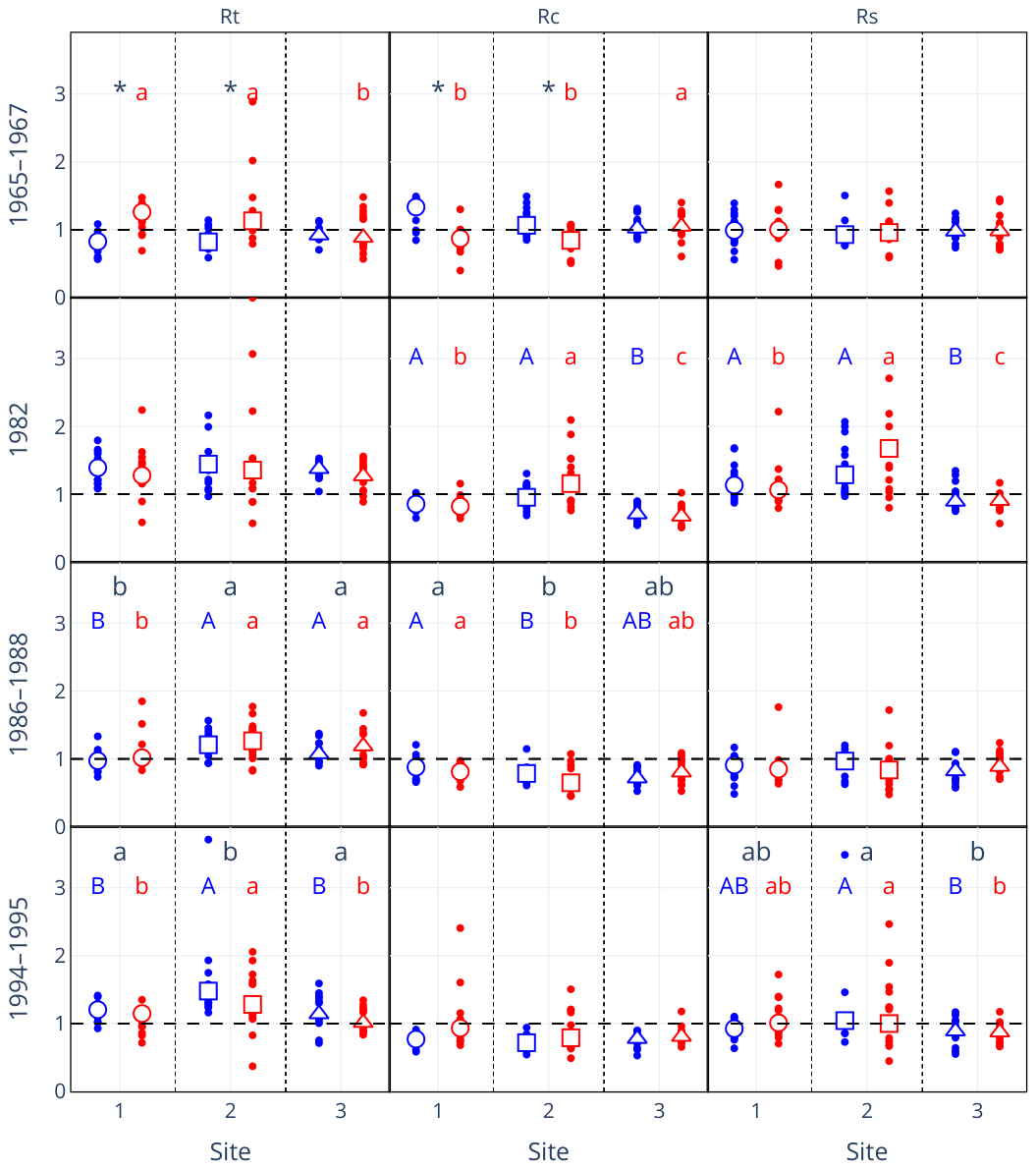
Across wet years, resistance, recovery, and resilience varied among events and sites, although many median values remained close to the reference value of 1 (Figure A1). In 1965–1967, R t and R c showed significant species × site interactions ( F 2 , 81 = 6.51, p = 0.002 and F 2 , 81 = 8.66, p < 0.001, respectively). Beech had higher R t but lower R c than oak at S1 and S2 (all p Holm < 0.001), whereas the species did not differ at S3. Within beech, R t was lower and R c higher at S3 than at S1 and S2, while no site differences occurred within oak. R s did not differ significantly between species or sites. In 1982, R t showed no significant effects, whereas R c and R s exhibited species × site interactions (p = 0.039 and p = 0.008, respectively). For both indices, S3 had the lowest values in oak, while beech followed the order S2 > S1 > S3; however, no species contrast was significant within an individual site. In 1986–1988, R t was lower at S1 than at S2 and S3, whereas R c was lower at S2 than at S1, with S3 being intermediate. Although R s showed a significant interaction (p = 0.029), none of the follow-up contrasts was significant. In 1994–1995, oak had higher R t than beech across sites (p = 0.011), and R t was highest at S2. Conversely, R c was higher in beech than in oak across sites (p < 0.001). R s was higher at S2 than at S3, with S1 being intermediate.
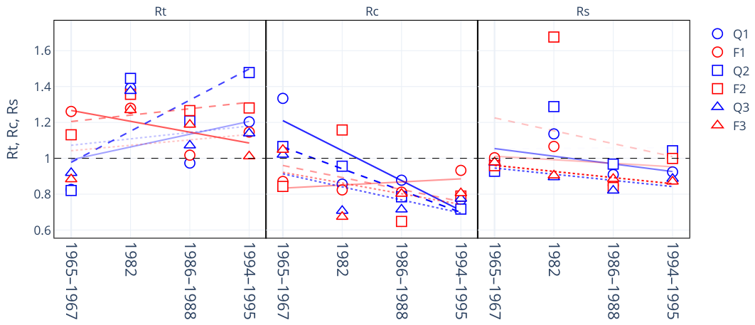
The trajectories in Figure A2 indicate temporal variability rather than a uniform increase in resistance. R t was comparatively low in 1965–1967, particularly for oak at S1 and S2, increased markedly in 1982, and subsequently remained relatively high at S2. At S1 and S3, however, resistance fluctuated among wet periods, and the highest values were often observed in 1982 rather than in 1994–1995.
Recovery generally declined from the early to the later wet periods, especially in oak. Oak R c decreased from values near or above 1 in 1965–1967 to values below 1 at all sites in 1994–1995. Beech recovery was more variable, including a temporary increase at S2 in 1982, but generally remained below 1 during the later periods. These patterns indicate that growth following wet events became progressively lower relative to pre-event growth, although the magnitude of the change depended on species and site.
Resilience showed no consistent temporal trend. Values were generally close to 1 in 1965–1967, followed by a pronounced but temporary increase at S2 in 1982, particularly in beech. During 1986–1988 and 1994–1995, resilience returned to values near or below 1, with the lowest values generally occurring at S3. Thus, the elevated resilience observed in 1982 represented an event- and site-specific response rather than a sustained temporal increase.
Figure A1. Resistance ( R t ), recovery ( R c ), and resilience ( R s ) for selected extreme wet events, calculated relative to the five years before and after each event for oak (blue) and beech (red) at all three sites. Open circles, squares, and triangles show site-level medians for Sites 1, 2, and 3, respectively, and colored dots represent individual trees. The horizontal dashed line marks the reference value of 1, where event-period growth equals mean pre-event growth for R t , mean post-event growth equals event-period growth for R c , and mean post-event growth equals mean pre-event growth for R s (see also Section 2). Species, site, and species × site effects were evaluated separately for each wet event and response variable using aligned rank transform factorial analyses of variance. Asterisks (*) indicate significant ART-C contrasts between oak and beech within a site. Colored letters indicate significant ART-C site contrasts within a species (uppercase for oak and lowercase for beech), whereas black letters indicate significant marginal site contrasts across species. Letters are displayed only when the corresponding site differences were significant. Follow-up p-values were adjusted using the Holm procedure; all symbols and letter groupings denote p < 0.05.
Forests 17 00909 g0a1
Figure A2. Median resistance ( R t ), recovery ( R c ), and resilience ( R s ) of oak (blue) and beech (red) during selected extreme wet years. Linear trends are shown as solid (Site 1), dashed (Site 2), and dotted (Site 3) colored lines. Brighter colors indicate more statistically significant linear trends.
Forests 17 00909 g0a2

References

  1. Allen, C.D.; Macalady, A.K.; Chenchouni, H.; Bachelet, D.; McDowell, N.; Vennetier, M.; Kitzberger, T.; Rigling, A.; Breshears, D.D.; Hogg, E.T.; et al. A global overview of drought and heat-induced tree mortality reveals emerging climate change risks for forests. For. Ecol. Manag. 2010, 259, 660–684. [Google Scholar] [CrossRef]
  2. Senf, C.; Buras, A.; Zang, C.S.; Rammig, A.; Seidl, R. Excess forest mortality is consistently linked to drought across Europe. Nat. Commun. 2020, 11, 6200. [Google Scholar] [CrossRef] [PubMed]
  3. Knutzen, F.; Averbeck, P.; Barrasso, C.; Bouwer, L.M.; Gardiner, B.; Grünzweig, J.M.; Hänel, S.; Haustein, K.; Johannessen, M.R.; Kollet, S.; et al. Impacts on and damage to European forests from the 2018–2022 heat and drought events. Nat. Hazards Earth Syst. Sci. 2025, 25, 77–117. [Google Scholar] [CrossRef]
  4. Gazol, A.; Camarero, J.J. Compound climate events increase tree drought mortality across European forests. Sci. Total Environ. 2022, 816, 151604. [Google Scholar] [CrossRef] [PubMed]
  5. Martínez-Sancho, E.; Treydte, K.; Lehmann, M.M.; Rigling, A.; Fonti, P. Drought impacts on tree carbon sequestration and water use–evidence from intra-annual tree-ring characteristics. New Phytol. 2022, 236, 58–70. [Google Scholar] [CrossRef] [PubMed]
  6. Rukh, S.; Sanders, T.G.M.; Krüger, I.; Schad, T.; Bolte, A. Distinct Responses of European Beech (Fagus sylvatica L.) to Drought Intensity and Length—A Review of the Impacts of the 2003 and 2018–2019 Drought Events in Central Europe. Forests 2023, 14, 248. [Google Scholar] [CrossRef]
  7. Bratu, I.; Dinca, L.; Constandache, C.; Murariu, G. Resilience and decline: The impact of climatic variability on temperate oak forests. Climate 2025, 13, 119. [Google Scholar] [CrossRef]
  8. Michelot, A.; Bréda, N.; Damesin, C.; Dufrêne, E. Differing growth responses to climatic variations and soil water deficits of Fagus sylvatica, Quercus petraea and Pinus sylvestris in a temperate forest. For. Ecol. Manag. 2012, 265, 161–171. [Google Scholar] [CrossRef]
  9. Stojanović, D.B.; Levanič, T.; Matović, B.; Stjepanović, S.; Orlović, S. Growth response of different tree species (oaks, beech and pine) from SE Europe to precipitation over time. Dendrobiology 2018, 79, 97–110. [Google Scholar] [CrossRef]
  10. Bohn, U.; Neuhäusl, R.; Gollub, G.; Hettwer, C.; Neuhäuslová, Z.; Raus, T.; Schlüter, H.; Weber, H. Map of the Natural Vegetation of Europe. Scale 1: 2,500,000; Landwirtschaftsverlag: Munster, Germany, 2003. [Google Scholar]
  11. Bohn, U.; Zazanashvili, N.; Nakhutsrishvili, G. The Map of the Natural Vegetation of Europe and its application in the Caucasus Ecoregion. Bull. Georgian Natl. Acad. Sci. 2007, 175, 112–121. [Google Scholar]
  12. Ellenberg, H.; Leuschner, C. Vegetation of Central Europe with the Alps: In Ecological, Dynamic, and Historical Perspective, 6th ed.; Verlag Eugen Ulmer: Stuttgart, Germany, 2010. [Google Scholar]
  13. Kroiher, F.; Schmitz, F. Tree Species Atlas for the Third National Forest Inventory (NFI 2012); Technical Report, Thünen Working Paper; Johann Heinrich von Thünen-Institut: Braunschweig, Germany, 2015. [Google Scholar]
  14. Institut National de L’Information Géographique et Forestière (IGN). Reference Guide—2025 Edition; IGN: Paris, France, 2025. [Google Scholar]
  15. Hipler, U. WET 2024—Forest Development Types Under Climate Change; Ministerium für Ernährung, Ländlichen Raum und Verbraucherschutz Baden-Württemberg: Stuttgart, Germany, 2024. [Google Scholar]
  16. HRSG (Ed.) Silvicultural Handbook: Principles and Guidelines for Near-Natural Management in the Hessian State Forest; Landesbetrieb HessenForst: Kassel, Germany, 2025. [Google Scholar]
  17. Scharnweber, T.; Manthey, M.; Wilmking, M. Differential radial growth patterns between beech (Fagus sylvatica L.) and oak (Quercus robur L.) on periodically waterlogged soils. Tree Physiol. 2013, 33, 425–437. [Google Scholar] [CrossRef] [PubMed]
  18. Vanhellemont, M.; Sousa-Silva, R.; Maes, S.L.; Van Den Bulcke, J.; Hertzog, L.; De Groote, S.R.; Van Acker, J.; Bonte, D.; Martel, A.; Lens, L.; et al. Distinct growth responses to drought for oak and beech in temperate mixed forests. Sci. Total Environ. 2019, 650, 3017–3026. [Google Scholar] [CrossRef] [PubMed]
  19. Vitasse, Y.; Bottero, A.; Cailleret, M.; Bigler, C.; Fonti, P.; Gessler, A.; Lévesque, M.; Rohner, B.; Weber, P.; Rigling, A.; et al. Contrasting resistance and resilience to extreme drought and late spring frost in five major European tree species. Glob. Change Biol. 2019, 25, 3781–3792. [Google Scholar] [CrossRef] [PubMed]
  20. Meyer, B.F.; Buras, A.; Rammig, A.; Zang, C.S. Higher susceptibility of beech to drought in comparison to oak. Dendrochronologia 2020, 64, 125780. [Google Scholar] [CrossRef]
  21. Schwarz, J.; Skiadaresis, G.; Kohler, M.; Kunz, J.; Schnabel, F.; Vitali, V.; Bauhus, J. Quantifying Growth Responses of Trees to Drought—A Critique of Commonly Used Resilience Indices and Recommendations for Future Studies. Curr. For. Rep. 2020, 6, 185–200. [Google Scholar] [CrossRef]
  22. Schroeder, H.; Nosenko, T.; Ghirardo, A.; Fladung, M.; Schnitzler, J.P.; Kersten, B. Oaks as Beacons of Hope for Threatened Mixed Forests in Central Europe. Front. For. Glob. Change 2021, 4, 670797. [Google Scholar] [CrossRef]
  23. Schmied, G.; Pretzsch, H.; Ambs, D.; Uhl, E.; Schmucker, J.; Fäth, J.; Biber, P.; Hoffmann, Y.D.; Šeho, M.; Mellert, K.H.; et al. Rapid beech decline under recurrent drought stress: Individual neighborhood structure and soil properties matter. For. Ecol. Manag. 2023, 545, 121305. [Google Scholar] [CrossRef]
  24. Enderle, L.; Gribbe, S.; Muffler, L.; Weigel, R.; Hertel, D.; Leuschner, C. A warmer climate impairs the growth performance of Central Europe’s major timber species in lowland regions. Sci. Total Environ. 2024, 941, 173665. [Google Scholar] [CrossRef] [PubMed]
  25. Schäffer, J.; Ehekircher, S.; Spangenberg, G.; Hein, S. Trees under Stress—What Will the Forests of the Future Look Like? Mitteilungen Dtsch. Bodenkd. Ges. 2025, 121, 63–81. [Google Scholar]
  26. Lloret, F.; Keeling, E.G.; Sala, A. Components of tree resilience: Effects of successive low-growth episodes in old ponderosa pine forests. Oikos 2011, 120, 1909–1920. [Google Scholar] [CrossRef]
  27. Palmer, W.C. Meteorological Drought; US Department of Commerce, Weather Bureau: Washington, DC, USA, 1965; Volume 30. [Google Scholar]
  28. Wells, N.; Goddard, S.; Hayes, M.J. A Self-Calibrating Palmer Drought Severity Index. J. Clim. 2004, 17, 2335–2351. [Google Scholar] [CrossRef]
  29. Van Der Schrier, G.; Barichivich, J.; Briffa, K.R.; Jones, P.D. A scPDSI-based global data set of dry and wet spells for 1901–2009. J. Geophys. Res. Atmos. 2013, 118, 4025–4048. [Google Scholar] [CrossRef]
  30. Zhou, Y.; Zhou, P.; Jin, J.; Wu, C.; Cui, Y.; Zhang, Y.; Tong, F. Drought identification based on Palmer drought severity index and return period analysis of drought characteristics in Huaibei Plain China. Environ. Res. 2022, 212, 113163. [Google Scholar] [CrossRef] [PubMed]
  31. Zink, M.; Samaniego, L.; Kumar, R.; Thober, S.; Mai, J.; Schäfer, D.; Marx, A. The German drought monitor. Environ. Res. Lett. 2016, 11, 074002. [Google Scholar] [CrossRef]
  32. Deutscher Wetterdienst. Hechingen Climate Station (Station ID 2074): Climate Data; Climate Data Center (CDC): Offenbach, Germany, 2026. [Google Scholar]
  33. Mauz, M.; Ehekircher, S.; Braun, A.; Niessner, A.; Schober, T.; Spangenberg, G.; Schäffer, J.; Hein, S.; Hochschild, V. Multi-scale and multi-compartment monitoring of tree vitality—Integrating soil, stem, crown, and remote sensing observations. Geosci. Instrum. Method. Data Syst. 2026, 15, 107–125. [Google Scholar] [CrossRef]
  34. Hein, S.; Ehekircher, S. DryTrees 360° Panoramas. Available online: https://36o.de/drytrees/ (accessed on 29 July 2026).
  35. Gillner, S.; Bräuning, A.; Roloff, A. Dendrochronological analysis of urban trees: Climatic response and impact of drought on frequently used tree species. Trees 2014, 28, 1079–1093. [Google Scholar] [CrossRef]
  36. Vremec, M.; Collenteur, R.A.; Birk, S. PyEt v1.3.1: A Python package for the estimation of potential evapotranspiration. Geosci. Model Dev. 2024, 17, 7083–7103. [Google Scholar] [CrossRef]
  37. Oudin, L. Search for a Relevant Potential Evapotranspiration Model as Input to a Lumped Rainfall–Runoff Model. Ph.D. Thesis, ENGREF (AgroParisTech), Paris, France, 2004. [Google Scholar]
  38. Dunn, R.J.H.; Blannin, J.; Willett, K.M.; Gobron, N.; Morris, G.A.; Ades, M.; Adler, R.; Alexe, M.; Allan, R.P.; Anderson, J.; et al. Global Climate. Bull. Am. Meteorol. Soc. 2025, 106, S11–S172. [Google Scholar] [CrossRef]
  39. Gärtner, H.; Nievergelt, D. The core-microtome: A new tool for surface preparation on cores and time series analysis of varying cell parameters. Dendrochronologia 2010, 28, 85–92. [Google Scholar] [CrossRef]
  40. Swetnam, T.L. dplPy: The Dendrochronology Program Library for Python. Python Software Package. 2024. Available online: https://github.com/OpenDendro/dplPy (accessed on 29 July 2026).
  41. Bunn, A.G. A dendrochronology program library in R (dplR). Dendrochronologia 2008, 26, 115–124. [Google Scholar] [CrossRef]
  42. Schweingruber, F.H. Der Jahrring: Standort, Methodik, Zeit und Klima in der Dendrochronologie [The Tree Ring]; Paul Haupt: Bern, Switzerland; Stuttgart, Germany, 1983; 234p. [Google Scholar]
  43. Schweingruber, F.H. Tree Rings: Basics and Applications of Dendrochronology; Springer Science & Business Media: Dordrecht, The Netherlands, 2012. [Google Scholar]
  44. Thurm, E.A.; Uhl, E.; Pretzsch, H. Mixture reduces climate sensitivity of Douglas-fir stem growth. For. Ecol. Manag. 2016, 376, 205–220. [Google Scholar] [CrossRef]
  45. Wobbrock, J.O.; Findlater, L.; Gergle, D.; Higgins, J.J. The Aligned Rank Transform for Nonparametric Factorial Analyses Using Only ANOVA Procedures. In Proceedings of the SIGCHI Conference on Human Factors in Computing Systems, Vancouver, BC, Canada, 7–12 May 2011; pp. 143–146. [Google Scholar]
  46. Elkin, L.A.; Kay, M.; Higgins, J.J.; Wobbrock, J.O. An Aligned Rank Transform Procedure for Multifactor Contrast Tests. In Proceedings of the 34th Annual ACM Symposium on User Interface Software and Technology, Virtual Event, 10–14 October 2021; pp. 754–768. [Google Scholar]
  47. McKinney, W. Data Structures for Statistical Computing in Python. SciPy 2010, 445, 51–56. [Google Scholar]
  48. Harris, C.R.; Millman, K.J.; Van Der Walt, S.J.; Gommers, R.; Virtanen, P.; Cournapeau, D.; Wieser, E.; Taylor, J.; Berg, S.; Smith, N.J.; et al. Array Programming with NumPy. Nature 2020, 585, 357–362. [Google Scholar] [CrossRef] [PubMed]
  49. Virtanen, P.; Gommers, R.; Oliphant, T.E.; Haberland, M.; Reddy, T.; Cournapeau, D.; Burovski, E.; Peterson, P.; Weckesser, W.; Bright, J.; et al. SciPy 1.0: Fundamental Algorithms for Scientific Computing in Python. Nat. Methods 2020, 17, 261–272. [Google Scholar] [CrossRef] [PubMed]
  50. Plotly Technologies Inc. Collaborative Data Science; Plotly Technologies Inc.: Montréal, QC, Canada, 2015. [Google Scholar]
  51. Deng, C.H. Timber Harvesting and Reforestation in the Federal Republic of Germany. Wirtschaftsdienst 1955, 35, 389–392. [Google Scholar]
  52. Kašpar, J.; Tumajer, J.; Altman, J.; Altmanová, N.; Čada, V.; Čihák, T.; Doležal, J.; Fibich, P.; Janda, P.; Kaczka, R.; et al. Major tree species of Central European forests differ in their proportion of positive, negative, and nonstationary growth trends. Glob. Change Biol. 2024, 30, e17146. [Google Scholar] [CrossRef] [PubMed]
  53. Scharnweber, T.; Manthey, M.; Criegee, C.; Bauwe, A.; Schröder, C.; Wilmking, M. Drought matters—Declining precipitation influences growth of Fagus sylvatica L. and Quercus robur L. in north-eastern Germany. For. Ecol. Manag. 2011, 262, 947–961. [Google Scholar] [CrossRef]
  54. Büntgen, U.; Esper, J.; Frank, D. How Do Trees Respond to Climate Change? Results of Dendroclimatological Studies. Jahrb. Baumpflege 2008, 2008, 26–39. [Google Scholar]
  55. Steckel, M.; Moser, W.K.; del Río, M.; Pretzsch, H. Implications of reduced stand density on tree growth and drought susceptibility: A study of three species under varying climate. Forests 2020, 11, 627. [Google Scholar] [CrossRef]
  56. Plauborg, K.U. Analysis of radial growth responses to changes in stand density for four tree species. For. Ecol. Manag. 2004, 188, 65–75. [Google Scholar] [CrossRef]
  57. Mattes, A. Growth and Competition in Mixed Beech/Oak Stands under Changing Climatic Conditions. Ph.D. Thesis, Albert-Ludwigs-Universität Freiburg, Freiburg im Breisgau, Germany, 2014. [Google Scholar] [CrossRef]
  58. Weber, P.; Bugmann, H.; Pluess, A.R.; Walthert, L.; Rigling, A. Drought response and changing mean sensitivity of European beech close to the dry distribution limit. Trees 2013, 27, 171–181. [Google Scholar] [CrossRef]
  59. González De Andrés, E.; Rosas, T.; Camarero, J.J.; Martínez-Vilalta, J. The intraspecific variation of functional traits modulates drought resilience of European beech and pubescent oak. J. Ecol. 2021, 109, 3652–3669. [Google Scholar] [CrossRef]
  60. Coble, A.P.; Vadeboncoeur, M.A.; Berry, Z.C.; Jennings, K.A.; McIntire, C.D.; Campbell, J.L.; Rustad, L.E.; Templer, P.H.; Asbjornsen, H. Are Northeastern US forests vulnerable to extreme drought? Ecol. Process. 2017, 6, 34. [Google Scholar] [CrossRef]
  61. DeSoto, L.; Cailleret, M.; Sterck, F.; Jansen, S.; Kramer, K.; Robert, E.M.; Aakala, T.; Amoroso, M.M.; Bigler, C.; Camarero, J.J.; et al. Low growth resilience to drought is related to future mortality risk in trees. Nat. Commun. 2020, 11, 545. [Google Scholar] [CrossRef] [PubMed]
  62. Hirsch, M.; Greiner-Müller, E.; Boden, S.; Hillenmeyer, K.; Mattes, A.; Schuler, J.; Spathelf, P.; Maaten, E.V.D.; Maaten-Theunissen, M.V.D.; Seifert, T. Drought and masting affect growth allocation along the stem axis in beech, oak, fir and spruce in temperate forests. Trees 2026, 40, 27. [Google Scholar] [CrossRef]
  63. Nussbaumer, A.; Gessler, A.; Benham, S.; de Cinti, B.; Etzold, S.; Ingerslev, M.; Jacob, F.; Lebourgeois, F.; Levanic, T.; Marjanović, H.; et al. Contrasting resource dynamics in mast years for European beech and oak—A continental scale analysis. Front. For. Glob. Change 2021, 4, 689836. [Google Scholar] [CrossRef]
  64. Hacket-Pain, A.J.; Lageard, J.G.; Thomas, P.A. Drought and reproductive effort interact to control growth of a temperate broadleaved tree species (Fagus sylvatica). Tree Physiol. 2017, 37, 744–754. [Google Scholar] [CrossRef] [PubMed]
  65. Hacket-Pain, A.; Foest, J.J.; Pearse, I.S.; LaMontagne, J.M.; Koenig, W.D.; Vacchiano, G.; Bogdziewicz, M.; Caignard, T.; Celebias, P.; Van Dormolen, J.; et al. MASTREE+: Time-series of plant reproductive effort from six continents. Glob. Change Biol. 2022, 28, 3066–3082. [Google Scholar] [CrossRef] [PubMed]
  66. Elling, W.; Dittmar, C.; Pfaffelmoser, K.; Rötzer, T. Dendroecological assessment of the complex causes of decline and recovery of the growth of silver fir (Abies alba Mill.) in Southern Germany. For. Ecol. Manag. 2009, 257, 1175–1187. [Google Scholar] [CrossRef]
  67. Castagneri, D.; Vacchiano, G.; Hacket-Pain, A.; DeRose, R.J.; Klein, T.; Bottero, A. Meta-analysis reveals different competition effects on tree growth resistance and resilience to drought. Ecosystems 2022, 25, 30–43. [Google Scholar] [CrossRef]
  68. Hein, S.; Dhôte, J.F. Effect of species composition, stand density and site index on the basal area increment of oak trees (Quercus sp.) in mixed stands with beech (Fagus sylvatica L.) in northern France. Ann. For. Sci. 2006, 63, 457–467. [Google Scholar] [CrossRef]
  69. Schmitt, A.; Trouvé, R.; Seynave, I.; Lebourgeois, F. Decreasing stand density favors resistance, resilience, and recovery of Quercus petraea trees to a severe drought, particularly on dry sites. Ann. For. Sci. 2020, 77, 52. [Google Scholar] [CrossRef]
  70. Merlin, M.; Perot, T.; Perret, S.; Korboulewsky, N.; Vallet, P. Effects of stand composition and tree size on resistance and resilience to drought in sessile oak and Scots pine. For. Ecol. Manag. 2015, 339, 22–33. [Google Scholar] [CrossRef]
Figure 2. Tree-ring widths of beech (red lines) and oak (blue lines) at the three study sites from 1920 to 2024. Light-colored lines represent individual trees, and darker colored lines represent mean tree-ring-width chronologies. Bottom panels show annual sample depth. Vertical dashed lines mark the year 1950.
Forests 17 00909 g002
Figure 3. Detrended site chronologies for beech (red lines) and oak (blue lines) along the three study sites from 1950 to 2024. RWI = Ring Width Index.
Forests 17 00909 g003
Figure 4. Correlation functions between monthly climate variables (scPDSI, SMI B S , precipitation [PP], and mean temperature [Tm]) and site chronologies (red: beech; blue: oak) from July of the previous year (JUL) to August of the current year (Aug). GS and gs represent the growing season (April–September) of the previous and current year, respectively. A and a represent the mean annual value (sum for PP) of the previous and current year, respectively. Vertical dashed lines separate correlation functions for each site and distinguish the previous year (uppercase letters) from the current year (lowercase letters). Correlations were calculated for 1950–2024 (n = 75), except for SMI B S , which covered 1951–2022 (n = 72). Filled bars indicate significant correlations at p < 0.05, whereas hollow bars indicate non-significant correlations. Other drought indices considered at this stage (PDSI, scPDSI s c h , and topsoil moisture index SMI T S ) were omitted from subsequent analyses because scPDSI and SMI B S showed consistently stronger correlations.
Forests 17 00909 g004
Figure 5. Pointer years of oak and beech across all sites and extreme dry and wet growing seasons based on the available scPDSI (1950–2024) and SMI B S (1951–2022) records. Pointer years are defined as years with an interval trend greater than 75%. Growing seasons (April–September) in which detrended scPDSI or SMI B S values fell below the 5th percentile or exceeded the 95th percentile are shown as extreme years. Both indices were linearly detrended to account for strong recent trends (see also Figure 1). Negative pointer years and extreme dry years are colored in darkred, positive pointer years and extreme humid years in teal. Selected extreme years/periods are highlighted accordingly.
Forests 17 00909 g005
Figure 6. Average growth deviation during drought events and the five years before and after each event at the three sites. Mean tree-ring width during the five years before the drought event was used as the reference. Oak is shown in blue and beech in red; filled areas indicate 90% bootstrap confidence intervals.
Forests 17 00909 g006
Figure 7. Resistance ( R t ), recovery ( R c ), and resilience ( R s ) for selected drought years, calculated relative to the five years before and after each event for oak (blue) and beech (red) at all three sites. Open circles, squares, and triangles show site-level medians for Sites 1, 2, and 3, respectively, and colored dots represent individual trees. The horizontal dashed line marks the reference value of 1, where event-year growth equals mean pre-event growth for R t , mean post-event growth equals event-year growth for R c , and mean post-event growth equals mean pre-event growth for R s (see also Section 2). Species, site, and species × site effects were evaluated separately for each drought event and response variable using aligned rank transform factorial analyses of variance. Asterisks (*) indicate significant ART-C contrasts between oak and beech within a site. Colored letters indicate significant ART-C site contrasts within a species (uppercase for oak and lowercase for beech), whereas black letters indicate significant marginal site contrasts across species. Letters are displayed only when the corresponding site differences were significant. Follow-up p-values were adjusted using the Holm procedure; all symbols and letter groupings denote p < 0.05. Omnibus test results are presented in Table A2.
Forests 17 00909 g007
Figure 8. Resistance ( R t ) versus recovery ( R c ) for each drought event. Blue and red symbols represent oak and beech, respectively. Circles, squares, and triangles denote Sites 1, 2, and 3, respectively. Open symbols show site-level medians, and filled symbols represent individual trees. The dashed line indicates resilience = 1.
Forests 17 00909 g008
Figure 9. Median resistance ( R t ), recovery ( R c ), resilience ( R s ), growth recovery time (GRT), increment loss due to drought (Loss), and average growth reduction (AGR) of oak (blue) and beech (red) for selected drought years. Open symbols show site-level medians. Linear trends are shown as solid (Site 1), dashed (Site 2), and dotted (Site 3) colored lines. Brighter colors indicate stronger statistical significance of the linear trend.
Forests 17 00909 g009
Table 1. Site characteristics, stand structure, tree dimensions, minimum tree age in 2025 (based on the oldest measured tree ring), mean tree-ring width, chronology statistics, and tree species composition. Values for tree-level variables are given as mean ± standard deviation, with n = 15 per species and site. AC: first-order autocorrelation on raw tree-ring series, Rbar: mean series correlation, MS: mean sensitivity, and EPS: Expressed Population Signal (Rbar, MS, and EPS on standardized ring-width values).
Site 1Site 2Site 3
Coordinates (WGS84)48.3691° N, 9.0004° E48.3634° N, 8.9948° E48.3690° N, 9.0460° E
Altitude [m a.s.l.]520550850
Slope [°]515–2040
Basal area [ m 2 ha 1 ]23.4339.9138.86
Density [stems ha 1 ]313520589
Average DBH [cm] (oak/beech)54.5 ± 10.4/43.1 ± 6.847.3 ± 10.8/37.3 ± 8.944.6 ± 10.5/42.1 ± 12.2
Average tree height [m] (oak/beech)29.5 ± 2.7/28.2 ± 2.423.4 ± 1.8/20.2 ± 3.817.4 ± 3.3/17.1 ± 2.8
Average minimum tree age in 2025 [years] (oak/beech)104.2 ± 38.7/87.0 ± 3.9111.9 ± 25.1/101.1 ± 6.4168.2 ± 30.0/149.4 ± 34.1
Average tree-ring width [mm] (oak/beech)2.30 ± 0.47/2.29 ± 0.341.73 ± 0.30/1.71 ± 0.401.09 ± 0.18/1.19 ± 0.21
AC (oak/beech)0.56 ± 0.16/0.78 ± 0.080.41 ± 0.19/0.68 ± 0.140.57 ± 0.27/0.63 ± 0.14
Rbar (oak/beech)0.42/0.380.59/0.310.49/0.45
MS (oak/beech)0.14/0.160.21/0.140.15/0.20
EPS (oak/beech)0.91/0.900.96/0.870.93/0.92
Tree species composition [%]Fagus sylvatica (78.3), Quercus petraea (8.0), Picea abies (8.0), Carpinus betulus (3.6), Tilia sp. (1.4), Pinus sylvestris (0.7)Fagus sylvatica (56.0), Quercus petraea (21.0), Carpinus betulus (10.0), Tilia sp. (6.0), Acer pseudoplatanus (3.5), Aria torminalis (3.5)Fagus sylvatica (56.0), Quercus petraea (12.8), Fraxinus excelsior (10.1), Sorbus aucuparia (7.3), Acer pseudoplatanus (7.3), Crataegus sp. (4.6), Acer campestre (1.8)
Soil propertiesVertic Cambisol on marl clay, periglacial cover with cambic horizon, clay-rich polyhedral subsoil, high nutrientHaplic Vertisol on marl clay, eroded and mixed profile with humus-rich polyhedral horizon, high nutrient availabilityRendzic Leptosol on limestone, shallow, skeletal, humus-rich topsoil, limited P and K availability
Table 2. Intercorrelation matrix (Pearson) of climate parameters and indices shown in Figure 1. Correlations were calculated for 1951–2022 (n = 72).
TmPPPDSIscPDSIscPDSIschSMITSSMIBS
Tm1−0.13−0.32−0.34−0.33−0.29−0.21
PP-10.800.620.480.780.61
PDSI--10.900.720.850.87
scPDSI---10.810.730.86
scPDSIsch----10.690.83
SMITS-----10.86
Table 3. List of extreme dry and wet years. Growing seasons were classified as extreme dry years when detrended scPDSI or detrended SMI B S values fell below the 5th percentile, and as extreme wet years when values exceeded the 95th percentile. SMI: Soil moisture index, scPDSI: self-calibrated Palmer Drought Severity Index.
Extreme Dry YearsClimate IndexExtreme Wet YearsClimate Index
1959SMI1965–1967SMI, scPDSI
1972SMI1982scPDSI
2004scPDSI1986–1988SMI, scPDSI
2017–2019SMI, scPDSI1994–1995SMI, scPDSI
Table 4. Site and species intercorrelations (Pearson) calculated for 1950–2024 (n = 75). Q and F denote oak (Quercus petraea) and beech (Fagus sylvatica), respectively; numerals identify Sites 1–3. Same-species chronologies were positively correlated across all site pairs, while within-site oak-beech correlations were strongest at Sites 2 and 3. n.s.: not significant, *: p < 0.05, **: p < 0.01, ***: p < 0.001.
Q2Q3F1F2F3
Q10.61 ***0.52 ***0.32 **0.25 *0.22 n.s.
Q210.57 ***0.31 **0.63 ***0.45 ***
Q3-10.46 ***0.39 ***0.66 ***
F1--10.54 ***0.54 ***
F2---10.56 ***
Table 5. Growth recovery time (GRT), increment loss due to drought (Loss), average growth reduction (AGR), and average recovery rate (ARR) for the selected drought events. Q and F denote oak (Quercus petraea) and beech (Fagus sylvatica), respectively; numerals identify Sites 1–3. Values are medians with interquartile ranges in brackets. Species, site, and species × site effects were evaluated separately for each drought event and response variable using aligned rank transform factorial analyses of variance. For significant interactions, bold values indicate significant ART-C species contrasts within a site, while different uppercase and lowercase letters indicate significant site contrasts within oak and beech, respectively. Follow-up p-values were adjusted using the Holm procedure. Omnibus test results are presented in Table A2.
Drought EventQ1F1Q2F2Q3F3
GRT [years]
19591.0 [1.0–1.8] A1.5 [1.0–2.0] a2.0 [1.0–4.0] A2.0 [2.0–5.5] a1.0 [1.0–1.5] A1.5 [1.0–2.5] a
19721.0 [1.0–1.0] A2.5 [2.0–3.0] a1.0 [1.0–1.0] A5.0 [3.0–6.0] a1.0 [1.0–1.8] A1.0 [1.0–2.5] b
20042.0 [1.0–2.5] B1.0 [1.0–3.0] b1.5 [1.0–2.0] B1.0 [1.0–3.0] b2.5 [2.0–4.0] A3.0 [2.5–3.5] a
2017–20191.0 [1.0–2.5] A2.0 [1.5–4.0] a2.0 [1.0–4.0] A3.0 [1.2–4.0] a1.0 [1.0–3.5] A1.0 [1.0–3.0] a
Loss [mm]
19590.00 [−0.16–0.26] A0.49 [−0.23–0.81] a−0.04 [−0.52–0.07] A−0.07 [−1.82–0.43] a0.20 [0.00–0.33] A0.08 [−0.26–0.51] a
19720.19 [−0.20–0.56] A−0.71 [−1.17–−0.10] b−0.13 [−0.36–0.12] A−1.93 [−3.89–−0.46] b0.22 [0.08–0.45] A0.13 [−0.30–0.56] a
20040.03 [−0.64–0.33] A−0.45 [−1.28–0.01] a−0.66 [−0.83–−0.30] A−0.67 [−0.85–0.52] a−0.28 [−0.34–−0.17] A−0.58 [−1.22–−0.32] a
2017–20190.09 [−0.86–0.26] AB−1.16 [−1.75–−0.40] ab−1.11 [−2.21–−0.05] B−2.62 [−3.53–−0.76] b−0.06 [−0.25–0.00] A−0.13 [−0.56–0.02] a
AGR [mm year 1 ]
19590.01 [−0.14–0.26] A0.37 [−0.12–0.81] a−0.04 [−0.19–0.07] A−0.03 [−0.34–0.30] a0.20 [0.03–0.33] A0.05 [−0.09–0.51] a
19720.19 [−0.16–0.50] AB−0.26 [−0.38–−0.05] ab−0.10 [−0.27–0.12] B−0.32 [−0.63–−0.15] b0.22 [0.05–0.45] A0.13 [−0.12–0.56] a
20040.01 [−0.26–0.23] A−0.29 [−0.56–0.01] a−0.35 [−0.56–−0.23] B−0.24 [−0.63–0.52] a−0.09 [−0.14–−0.07] A−0.21 [−0.35–−0.13] a
2017–20190.09 [−0.28–0.26] AB−0.53 [−0.53–−0.22] ab−0.24 [−0.66–−0.05] B−0.88 [−0.90–−0.52] b−0.05 [−0.12–−0.00] A−0.13 [−0.26–0.01] a
ARR [%]
19594.33 [−1.29–6.57] A−5.08 [−21.34–−0.56] a3.47 [−0.90–8.42] A2.59 [0.29–4.44] a−3.08 [−9.85–0.13] A−0.16 [−10.09–2.39] a
1972−0.19 [−6.13–3.60] B4.48 [2.26–6.80] a11.45 [5.40–20.04] A3.55 [1.42–7.17] a−12.35 [−26.73–−1.11] C1.73 [−6.84–7.71] a
2004−0.16 [−3.82–10.47] B11.36 [3.30–17.16] a24.99 [18.12–28.33] A9.24 [1.64–40.13] a5.70 [1.40–9.41] B13.86 [9.49–15.38] a
2017–20192.15 [−2.52–4.04] B8.10 [3.64–12.32] b7.41 [5.65–14.87] A13.06 [10.79–14.70] a2.75 [2.11–6.26] B5.27 [−5.58–10.45] b
Disclaimer/Publisher’s Note: The statements, opinions and data contained in all publications are solely those of the individual author(s) and contributor(s) and not of MDPI and/or the editor(s). MDPI and/or the editor(s) disclaim responsibility for any injury to people or property resulting from any ideas, methods, instructions or products referred to in the content.