Spatial Patterns and Influencing Factors of Forest Net Ecosystem Productivity in the Middle and Upper Reaches of the Ganjiang River Basin

Abstract

Net ecosystem productivity (NEP) reflects the net carbon balance of forest ecosystems and is widely used to evaluate their carbon sink capacity. For the Ganjiang River Basin, identifying where forest NEP is high or low and explaining its controlling factors can support more targeted carbon sink management. However, under complex environmental conditions, the nonlinear responses of NEP and the differences among vegetation types are still not fully clear. In this study, forest NEP in the middle and upper reaches of the Ganjiang River Basin was estimated for 2023. An XGBoost–SHAP framework was then used to examine the effects of climatic, topographic, and stand structural factors and to identify possible threshold responses. The results showed that forest NEP had clear spatial differences. High NEP values were mainly distributed in peripheral areas, whereas low values were concentrated in the central region. The spatial distribution also showed significant positive autocorrelation. At the regional scale, elevation (DEM), mean annual temperature (TEMP), and vapor pressure deficit (VPD) were the dominant factors affecting NEP. However, the main drivers varied among different vegetation types. The SHAP results further indicated that several factors had nonlinear threshold effects. Precipitation showed an inhibitory effect within 1400–1680 mm, and VPD showed a similar negative response within 0.48–0.54 kPa. These results help explain the formation of regional forest carbon sinks and provide a reference for forest-type-specific ecological management.

1. Introduction

Over the past few decades, the continuous increase in greenhouse gas emissions has intensified global warming [1]. This change has placed growing pressure on ecological security and sustainable development worldwide [2]. Under China’s carbon peaking and carbon neutrality targets, improving the carbon sequestration capacity of terrestrial ecosystems has become an important way to support climate change mitigation [3]. Forests are a major carbon pool in terrestrial ecosystems. They participate directly in the global carbon cycle and have strong potential for carbon sequestration [4,5,6]. Elucidating the spatial distribution of forest net ecosystem productivity (NEP) and its controlling drivers is, therefore, important for understanding regional carbon cycle processes and developing targeted forest carbon sink management strategies.

To evaluate carbon dynamics, metrics such as gross primary productivity (GPP) are utilized alongside net primary productivity (NPP) and net ecosystem productivity (NEP). Among these indicators, NEP represents the balance between ecosystem productivity and total ecosystem respiration. It directly reflects the net exchange of carbon between ecosystems and the overlying atmosphere. Consequently, NEP provides a definitive measure of whether an ecosystem functions as a carbon sink or a carbon source. Current carbon sink estimation methods can generally be classified into four categories [7,8]: plot-based inventory methods [9], eddy covariance measurements [10], atmospheric inversion methods [11], and remote sensing–based model simulations [12]. Although field inventory methods provide high accuracy, their high labor costs limit their application for large-scale and long-term continuous monitoring. Similarly, although eddy covariance measurements can provide accurate carbon flux observations at specific sites, sparse station distribution constrains their extrapolation to regional scales [13]. In contrast, remote sensing–based model simulations have become an important approach for estimating carbon sinks and ecosystem productivity at medium to large spatial scales because of their broad spatiotemporal coverage and high computational efficiency. Among these models, the Carnegie–Ames–Stanford Approach (CASA), a typical light-use efficiency model, has been widely applied to simulate the spatiotemporal dynamics of net primary productivity (NPP) by integrating vegetation physiological processes with abiotic variables, including temperature, precipitation, and solar radiation [14,15]. However, NPP mainly reflects the net production capacity of vegetation after autotrophic respiration has been deducted, and therefore cannot directly represent the net carbon balance of an ecosystem. Net ecosystem productivity (NEP) is commonly defined as the difference between NPP and heterotrophic respiration (R_h) [16,17]. Based on this theoretical framework, this study estimated forest NPP in the middle and upper reaches of the Ganjiang River Basin using the CASA model, high-resolution remote sensing imagery, and meteorological data. Heterotrophic respiration was then estimated to calculate forest NEP, which was used to analyze the forest carbon sink status and its spatial distribution characteristics within the study region.

Clarifying the spatial pattern of forest NEP together with its controlling factors is important for regional carbon management. It is also necessary to examine how these factors interact with each other. Previous studies have often used correlation analysis, multiple linear regression, and geographic detector methods to analyze the environmental factors affecting NEP [18,19,20,21]. However, these traditional statistical approaches often assume linear relationships and, therefore, struggle to capture the complex nonlinear responses and threshold effects induced by environmental changes and human activities [22]. To overcome these limitations, machine learning (ML) provides robust nonlinear mapping and high-dimensional data modeling capabilities. ML can effectively process complex ecological datasets without relying on the strict biophysical assumptions required by traditional process-based models [23,24,25]. Furthermore, to address the limitations of treating complex machine learning models as black boxes, post-hoc interpretability techniques are increasingly adopted. Among these, Shapley additive explanations (SHAP), grounded in cooperative game theory, quantify the marginal contribution of individual features. This approach enables transparent characterization of nonlinear response relationships and interaction effects among drivers [26,27], thereby substantially improving model interpretability and providing deeper insights into ecological mechanisms.

The spatial patterns of forest NEP and their driving mechanisms were analyzed in the middle and upper reaches of the Ganjiang River Basin. Several widely used machine-learning algorithms were compared, and XGBoost (version 3.1.1) was selected as the best-performing model for subsequent SHAP-based driving-factor analysis. Using SHAP, we quantified the relative importance of climatic, topographic, and stand structural factors, and further explored their nonlinear responses and interaction effects on NEP. Based on these analyses, we identified the dominant environmental drivers of forest NEP and quantified their non-linear threshold effects. The results are expected to contribute to regional carbon sink management and the development of targeted forest carbon sequestration and ecological regulation strategies.

2. Materials and Methods

2.1. Overview of the Study Area

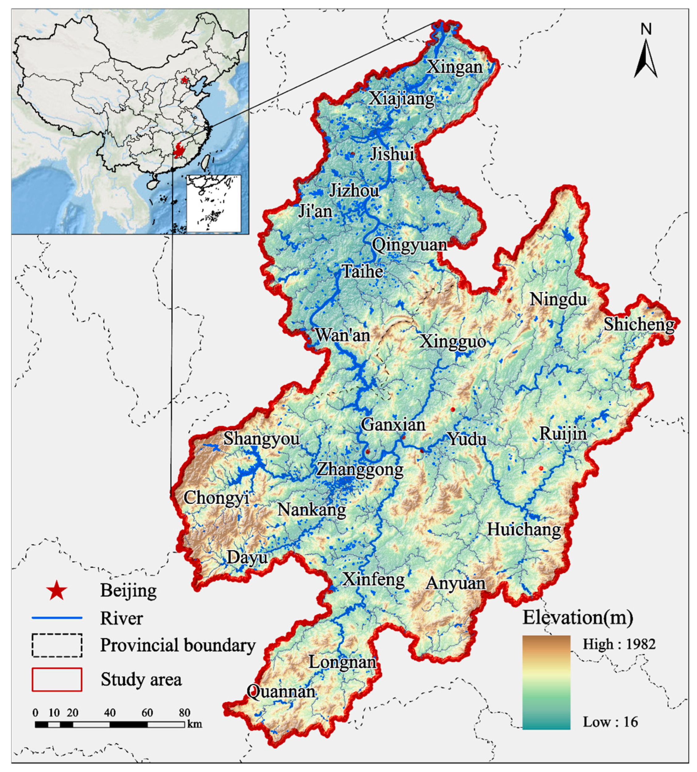
The research area in this study is located in the middle and upper reaches of the Ganjiang River Basin (25°29′ N–27°57′ N, 114°15′ E–116°37′ E) (Figure 1), located in the south-central region of Jiangxi Province and covering an area of approximately 38,200 km². Administratively, the region comprises 24 county-level administrative units within the jurisdictions of Ganzhou and Ji’an municipalities. Specifically, the upper reaches consist of 16 counties and districts (including Nankang, Zhanggong, and Xinfeng), whereas the middle-reach corridor includes eight county-level divisions (Jizhou, Qingyuan, Ji’an, Taihe, Wan’an, Jishui, Xiajiang, and Xingan). Topographically, the region is characterized by a landscape pattern of surrounding mountains and a longitudinal river valley. The eastern, southern, and northwestern margins are bordered by the branch ranges of the Wuyi, Nanling, and Luoxiao Mountains [28], respectively. In contrast, the central area forms a ribbon-like alluvial plain along the main channel of the Ganjiang River. Climatically, the region falls within the mid-subtropical monsoon climate zone, characterized by abundant precipitation and favorable thermal conditions. The dominant vegetation type is subtropical evergreen broad-leaved forest, which is widely distributed across the mountainous and hilly areas, particularly in the Wuyi and Jiulian mountain ranges [29].

2.2. Data Sources and Preprocessing

According to the characteristics of the study area and the needs of NEP estimation and driving-factor analysis, this study collected data on hydrothermal conditions, topography, and forest biophysical attributes (

Table 1. Summary of major data types and data sources.

Variable	Abbreviation	Unit	Data Source (Processing Method)
Geomorphological type	GEOM	-	Geomorphological Atlas of the People’s Republic of China [30]
Elevation	DEM	m	Geospatial Data Cloud (http://www.gscloud.cn/, accessed on 5 May 2026)
Slope	SLOPE	°	Calculated from DEM
Annual precipitation	PRE	mm	China Meteorological Data Service Centre (http://data.cma.cn, accessed on 5 May 2026)
Vapor pressure deficit	VPD	kPa
Mean annual temperature	TEMP	°C
Sunshine duration	SSD	h
Age group	AGE	-	Forestry Department of Jiangxi Province
Soil depth	SD	cm
Stand volume	VOL	m3 hm−2
Canopy density	CD	0–1
Vegetation type	VType	-
Normalized difference vegetation index	NDVI	-	https://earthexplorer.usgs.gov/, accessed on 5 May 2026

). To ensure spatial consistency, all datasets were projected to the WGS 1984 UTM Zone 50N coordinate system and then resampled to a 250 m × 250 m resolution.

2.3. Methodology

2.3.1. Estimation of NPP

The Carnegie–Ames–Stanford Approach (CASA) model was used to estimate vegetation net primary productivity (NPP) [31]. CASA is a light-use efficiency model driven by remote sensing and climate data. In the CASA model, vegetation NPP is calculated based on absorbed photosynthetically active radiation (APAR) and light-use efficiency $\left(\mathsf{\epsilon }\right)$. APAR quantifies the portion of photosynthetically active radiation captured by vegetation canopies, while $\mathsf{\epsilon }$ reflects the efficiency with which vegetation converts absorbed radiation into biomass.

$$\mathrm{NPP}\left(\mathrm{x},\mathrm{t}\right)=\mathrm{APAR}\left(\mathrm{x},\mathrm{t}\right)\times \mathsf{\epsilon }\left(\mathrm{x},\mathrm{t}\right)$$

(1)

where $\mathrm{x}$ denotes the pixel location, n and $\mathrm{t}$ denotes the time step. $\mathrm{NPP}(\mathrm{x},\mathrm{t})$ represents net primary productivity, $\mathrm{APAR}(\mathrm{x},\mathrm{t})$ represents absorbed photosynthetically active radiation, and $\mathsf{\epsilon }(\mathrm{x},\mathrm{t})$ represents actual light use efficiency.

APAR was calculated as follows:

$$\mathrm{APAR}\left(\mathrm{x},\mathrm{t}\right)=\mathrm{SOL}\left(\mathrm{x},\mathrm{t}\right)\times \mathrm{FPAR}\left(\mathrm{x},\mathrm{t}\right)\times 0.5$$

(2)

where SOL(x,t) is total solar radiation, and FPAR(x,t) is the fraction of photosynthetically active radiation absorbed by vegetation. The coefficient 0.5 indicates that photosynthetically active radiation accounts for about half of total solar radiation, corresponding to the wavelength range of 0.38–0.71 μm [32,33].

Actual light use efficiency was adjusted by temperature and moisture stress factors as follows:

$${\mathsf{\epsilon }}_{\left(\mathrm{x},\mathrm{t}\right)}={\mathrm{T}}_{\mathsf{\epsilon }1\left(\mathrm{x},\mathrm{t}\right)}\times {\mathrm{T}}_{\mathsf{\epsilon }2\left(\mathrm{x},\mathrm{t}\right)}\times {\mathrm{W}}_{\mathsf{\epsilon }\left(\mathrm{x},\mathrm{t}\right)}\times {\mathsf{\epsilon }}_{\max }$$

(3)

where ${\mathsf{\epsilon }}_{\max }$ is the maximum light use efficiency under ideal conditions. ${\mathrm{T}}_{\mathsf{\epsilon }1}$ and ${\mathrm{T}}_{\mathsf{\epsilon }2}$ represent temperature stress coefficients, and ${\mathrm{W}}_{\mathsf{\epsilon }}$ represents the water limitation factor. For different vegetation types, the ${\mathsf{\epsilon }}_{\max }$ values were obtained from Zhu et al. [34].

2.3.2. Estimation of NEP

The heterotrophic respiration $\left({\mathrm{R}}_{\mathrm{h}}\right)$ was calculated using an empirical equation driven by temperature and precipitation [35,36]. This approach has been applied in previous studies on the carbon cycle and is suitable for estimating soil respiration at regional scales. The equation is expressed as

$${\mathrm{R}}_{\mathrm{h}}=3.069\left({\mathrm{e}}^{0.0912·\mathrm{T}}+\ln \left(0.3145·\mathrm{R}+1\right)\right)$$

(4)

where ${\mathrm{R}}_{\mathrm{h}}$ represents heterotrophic respiration, $\mathrm{T}$ is air temperature, and $\mathrm{R}$ is precipitation. All input variables were kept at the same temporal scale. Monthly values were first processed and then aggregated to obtain annual ${\mathrm{R}}_{\mathrm{h}}$.

Forest NEP was calculated by subtracting heterotrophic respiration from NPP [37] as follows:

$$\mathrm{NEP}=\mathrm{NPP}-{\mathrm{R}}_{\mathrm{h}}$$

(5)

A positive NEP value indicates net carbon uptake by the ecosystem, meaning that the ecosystem functions as a carbon sink. In contrast, a negative NEP value indicates net carbon release and represents a carbon source. When NEP equals zero, carbon uptake and carbon release are approximately balanced.

2.3.3. Spatial Autocorrelation Analysis

Spatial clustering patterns of forest NEP were examined using spatial autocorrelation analysis. Global Moran’s I was employed to assess the overall spatial dependence of NEP [38,39,40,41]. A positive Moran’s I value indicates that similar NEP values tend to be clustered in space, while a negative value indicates spatial dispersion.

Local clustering characteristics were further analyzed using the Local Indicators of Spatial Association (LISA) approach. At the grid-cell scale, Local Moran’s ${\mathrm{I}}_{\mathrm{i}}$ was calculated to identify spatial clusters such as high–high and low–low types. The corresponding formulations are given below:

$${\mathrm{Moran}}^{’}\mathrm{s} \mathrm{I}={\displaystyle \frac{\mathrm{n}{\sum }_{\mathrm{i}=1}^{\mathrm{n}}{\sum }_{\mathrm{j}=1}^{\mathrm{n}}{\mathrm{w}}_{\mathrm{ij}}\left({\mathrm{x}}_{\mathrm{i}}-\overline{\mathrm{x}}\right)\left({\mathrm{x}}_{\mathrm{j}}-\overline{\mathrm{x}}\right)}{\left({\sum }_{\mathrm{i}=1}^{\mathrm{n}}{\sum }_{\mathrm{j}=1}^{\mathrm{n}}{\mathrm{w}}_{\mathrm{ij}}\right){\sum }_{\mathrm{i}=1}^{\mathrm{n}}{\left({\mathrm{x}}_{\mathrm{i}}-\overline{\mathrm{x}}\right)}^2}}$$

(6)

$${\mathrm{Moran}}^{’}\mathrm{s} {\mathrm{I}}_{\mathrm{i}}={\displaystyle \frac{\left({\mathrm{x}}_{\mathrm{i}}-\overline{\mathrm{x}}\right)}{{\mathrm{m}}_0}}{\sum }_{\mathrm{j}=1}^{\mathrm{n}}{\mathrm{w}}_{\mathrm{ij}}\left({\mathrm{x}}_{\mathrm{j}}-\overline{\mathrm{x}}\right)$$

(7)

$$\widehat{{\mathrm{m}}_0}={\displaystyle \frac{{\sum }_{\mathrm{i}=1}^{\mathrm{n}}{\left({\mathrm{x}}_{\mathrm{i}}-\overline{\mathrm{x}}\right)}^2}{\mathrm{n}}}$$

(8)

where n denotes the total number of spatial units. x_i and x_j represent the NEP values of spatial units i and j, respectively. $\overline{\mathrm{x}}$ indicates the mean NEP value. w_ij is the spatial weight matrix; and m₀ represents the variance.

To rigorously evaluate the statistical significance of these local spatial associations, Monte Carlo permutation tests were employed. This procedure calculates the standardized Z-score for the local Moran’s I_i as follows:

$$\mathrm{Z}\left({\mathrm{I}}_{\mathrm{i}}\right)={\displaystyle \frac{{\mathrm{I}}_{\mathrm{i}}-\mathrm{E}\left[{\mathrm{I}}_{\mathrm{i}}\right]}{\sqrt{\mathrm{Var}\left[{\mathrm{I}}_{\mathrm{i}}\right]}}}$$

(9)

where E[I_i] is the expected value of ${\mathrm{I}}_{\mathrm{i}}$, and Var[I_i] is its variance. At a predetermined significance level ($\mathsf{\alpha }$ = 0.05), a spatial pattern is deemed statistically significant if |Z| > 1.96 and p < 0.05; conversely, values falling outside these thresholds imply a random spatial distribution. Ultimately, LISA cluster maps were combined with significance level (p-value) maps to delineate core clustering areas with high statistical confidence.

2.3.4. Pearson Correlation Analysis

Pearson correlation analysis was conducted to assess the linear relationships between forest NEP and potential driving factors [42,43,44]. This analysis provides a preliminary understanding of the direction and strength of the relationship between variables before model-based attribution analysis. The Pearson correlation coefficient $\mathrm{R}$ was calculated as follows:

$$\mathrm{R}={\displaystyle \frac{{\sum }_{\mathrm{i}=1}^{\mathrm{n}}\left({\mathrm{x}}_{\mathrm{i}}-\overline{\mathrm{x}}\right)\left({\mathrm{y}}_{\mathrm{i}}-\overline{\mathrm{y}}\right)}{\sqrt{{\sum }_{\mathrm{i}=1}^{\mathrm{n}}{\left({\mathrm{x}}_{\mathrm{i}}-\overline{\mathrm{x}}\right)}^2}\sqrt{{\sum }_{\mathrm{i}=1}^{\mathrm{n}}{\left({\mathrm{y}}_{\mathrm{i}}-\overline{\mathrm{y}}\right)}^2}}}$$

(10)

where $\mathrm{n}$ is the number of samples. ${\mathrm{x}}_{\mathrm{i}}$ and ${\mathrm{y}}_{\mathrm{i}}$ represent the NEP value and the corresponding value of a driving factor at the $\mathrm{i}$-th sample, respectively. $\overline{\mathrm{x}}$ and $\overline{\mathrm{y}}$ are their mean values. The coefficient ranges from −1 to 1. A value close to 1 indicates a strong positive linear relationship, a value close to −1 indicates a strong negative linear relationship, and a value near 0 indicates a weak linear relationship [45].

2.3.5. Machine Learning Model Construction and Selection

Machine-learning models were constructed to investigate the driving mechanisms of forest NEP by characterizing the relationships between NEP and potential explanatory variables. Three commonly used ensemble learning algorithms were selected: Random Forest, XGBoost, and LightGBM [46,47,48]. These models differ in their learning strategies and model structures, and they are suitable for capturing nonlinear relationships in complex ecological data. Their main principles and applicability are summarized in

Table 2. Main principles and applicability of the machine-learning models used in this study.

Model	Main Assumptions & Principles	Applicable Scope & Advantages
Random Forest	Based on the Bagging strategy; requires no strict assumptions regarding data distribution; constructs multiple decision trees for parallel computation, utilizing random sampling and random feature selection to reduce model variance.	Suitable for high-dimensional, non-linear, and noisy datasets; demonstrates strong resistance to overfitting and is insensitive to outliers; however, in regression tasks, it may fail to predict values beyond the range of the training set.
LightGBM	The model is based on a gradient boosting decision tree (GBDT) framework and utilizes a histogram-based decision tree algorithm, as well as Gradient-based One-Side Sampling (GOSS) and Exclusive Feature Bundling (EFB) techniques.	Particularly well suited for large-scale, high-dimensional massive data; features exceptionally fast training speeds and low memory consumption
XGBoost	The boosting strategy relies on a second-order Taylor approximation of the loss function, while regularization is introduced to reduce model complexity.	Ideal for scenarios requiring high predictive accuracy; supports parallel computation and exhibits strong capability in handling sparse data

.

To compare the models under consistent conditions, Bayesian optimization was used to tune the key hyperparameters of each algorithm. A five-fold cross-validation strategy was adopted during model training. In each round, four subsets were used for training, while the remaining subset served as validation. Model performance was evaluated in terms of the coefficient of determination (R²), root mean square error (RMSE), and mean absolute error (MAE), and the metrics were averaged across all rounds [49].

2.3.6. Model Performance Evaluation

Model performance was assessed using three metrics: root mean square error (RMSE), mean absolute error (MAE), and the coefficient of determination $\left({\mathrm{R}}^2\right)$. RMSE and MAE were used to measure the prediction error, while ${\mathrm{R}}^2$ was used to describe the explanatory ability of the model. Lower RMSE and MAE values indicate smaller errors, and a higher ${\mathrm{R}}^2$ value indicates better model performance. These metrics were calculated as follows [50,51]:

$$\mathrm{RMSE}=\sqrt{{\displaystyle \frac{1}{\mathrm{n}}}{\sum }_{\mathrm{i}=1}^{\mathrm{n}}{\left({\mathrm{y}}_{\mathrm{i}}-\widehat{{\mathrm{y}}_{\mathrm{i}}}\right)}^2}$$

(11)

$$\mathrm{MAE}={\displaystyle \frac{1}{\mathrm{n}}}{\sum }_{\mathrm{i}=1}^{\mathrm{n}}\left|{\mathrm{y}}_{\mathrm{i}}-\widehat{{\mathrm{y}}_{\mathrm{i}}}\right|$$

(12)

$${\mathrm{R}}^2=1-\left({\displaystyle \frac{{\sum }_{\mathrm{i}=1}^{\mathrm{n}}{\left(\widehat{{\mathrm{y}}_{\mathrm{i}}}-{\mathrm{y}}_{\mathrm{i}}\right)}^2}{{\sum }_{\mathrm{i}=1}^{\mathrm{n}}{\left(\overline{\mathrm{y}}-{\mathrm{y}}_{\mathrm{i}}\right)}^2}}\right)$$

(13)

where n represents the total number of samples; $\overline{\mathrm{y}}$ is the mean value of the variable y; and $\widehat{{\mathrm{y}}_{\mathrm{i}}}$ denotes the predicted value of the variable y.

2.3.7. Shapley Additive Explanations (SHAP) Analysis

SHAP was employed to interpret the contribution of individual driving factors to the model output. It is based on Shapley values from cooperative game theory, where each input variable is assigned an importance value according to its contribution to model predictions. SHAP was employed to quantify how climatic, topographic, and stand structural variables affect forest NEP in this study. It was also used to identify nonlinear responses and interaction effects among the driving factors.

The Shapley value of feature $\mathrm{i}$ was calculated as follows:

$${\mathsf{\varphi }}_{\mathrm{i}}={\sum }_{\mathrm{S}\subseteq \mathrm{N}\setminus \left\{\mathrm{i}\right\}}{\displaystyle \frac{\left|\mathrm{S}\right|!\left(\mathrm{N}-\left|\mathrm{S}\right|-1\right)!}{\mathrm{N}!}}\left[\mathrm{f}\left(\mathrm{S}\cup \left\{\mathrm{i}\right\}\right)-\mathrm{f}\left(\mathrm{S}\right)\right]$$

(14)

where ${\mathsf{\varphi }}_{\mathrm{i}}$ is the SHAP value of feature $\mathrm{i}$, $\mathrm{N}$ represents the full set of input features, and $\mathrm{S}$ is a subset of features that does not include feature $\mathrm{i}$. $\mathrm{f}\left(\mathrm{S}\right)$ represents the model output using the feature subset $\mathrm{S}$, while $\mathrm{f}(\mathrm{S}\cup \{\mathrm{i}\left\}\right)$ represents the model output after feature $\mathrm{i}$ is added. SHAP values were calculated using the SHAP Python 3.13 package based on the selected XGBoost model.

2.3.8. Methodological Framework

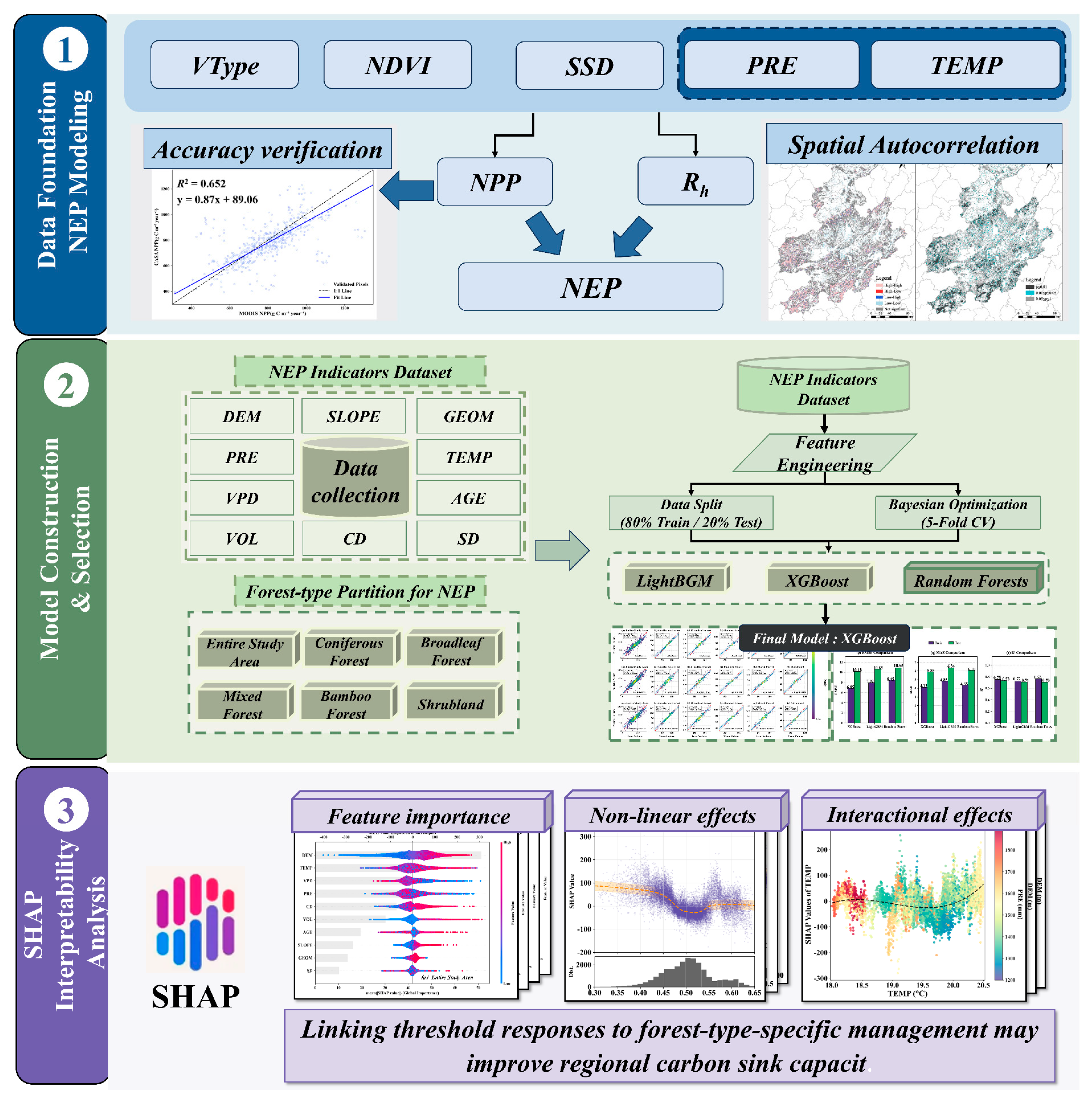
The workflow of this study is presented in Figure 2. First, forest NEP in the middle and upper reaches of the Ganjiang River Basin was estimated by integrating remote sensing variables, meteorological characteristics, topographic factors, and stand structural attributes. Then, the spatial distribution of NEP was analyzed using spatial statistical methods. After that, three machine-learning models were compared to identify the most suitable one for characterizing how forest NEP responds to potential influencing factors. Based on the selected model, SHAP analysis was used to identify the main drivers of forest NEP, examine nonlinear threshold responses, and explore interaction effects among key variables. This workflow was designed to support forest-type-specific interpretation of regional carbon sink patterns.

3. Results and Analysis

3.1. Estimation Results and Accuracy Evaluation of NPP

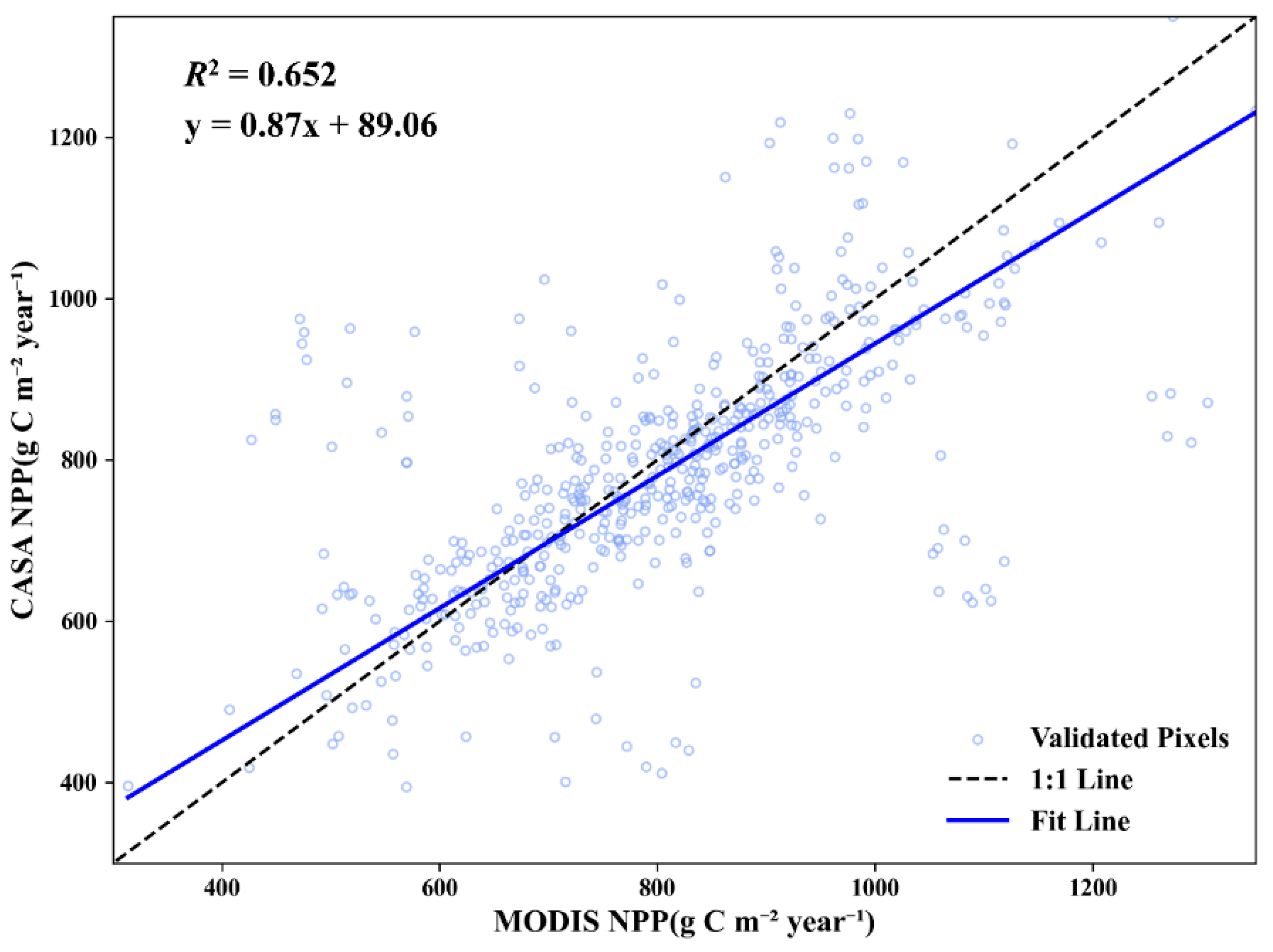
The mean NPP in the study area was estimated at 817.39 g C m⁻² year⁻¹, which was comparable to the results reported by Wen et al. [52]. The estimated NPP was validated against the 2023 MOD17A3HGF product. The results showed that the CASA-simulated NPP was generally consistent with the MODIS-derived product in spatial variation and magnitude, with a significant correlation (R² = 0.652, p < 0.001). These results indicate that the CASA model produced reliable estimates and is suitable for NPP estimation in the study area (Figure 3).

3.2. Estimation Results and Spatial Distribution Characteristics of NEP

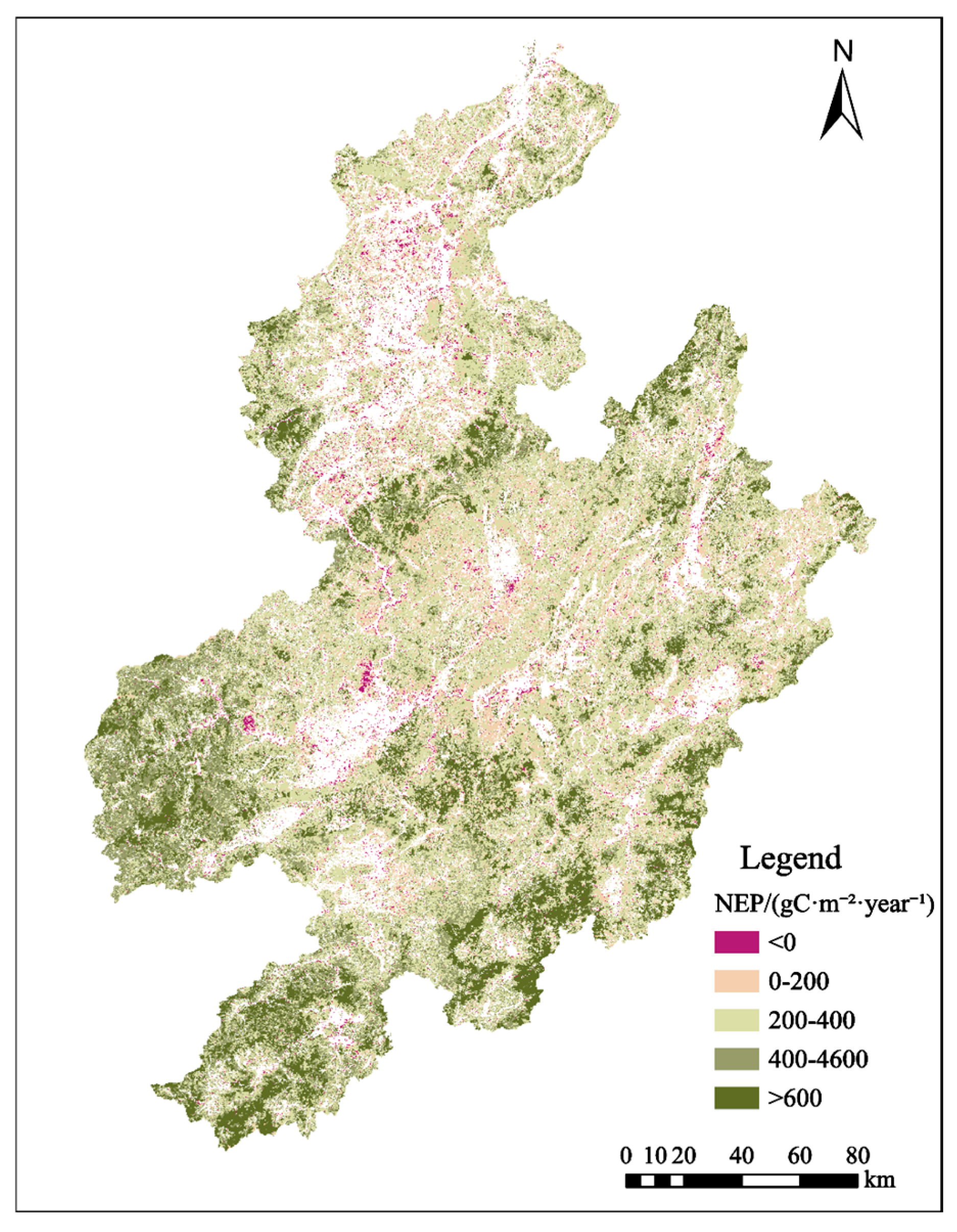
The average forest NEP in the study area in 2023 was 426.66 g C m⁻² year⁻¹. This value was close to that reported by Zheng et al. for middle subtropical forest ecosystems (441.91 g C m⁻² year⁻¹) [53]. Forest NEP showed clear spatial distribution characteristics in the study area (Figure 4). In general, higher NEP values were concentrated in mountainous regions at the periphery, whereas lower values were primarily distributed in the central river valley plains. High-value zones were concentrated in the Luoxiao and Nanling Mountains, mainly located in the southwestern, southern, and northwestern regions of the study area, including Chongyi and Quannan. By comparison, low-value zones appeared in strip-like or patchy forms along the Ganjiang River valley plain and within the Jitai Basin, such as Jizhou District. Overall, NEP increased gradually from plain areas toward mountainous regions.

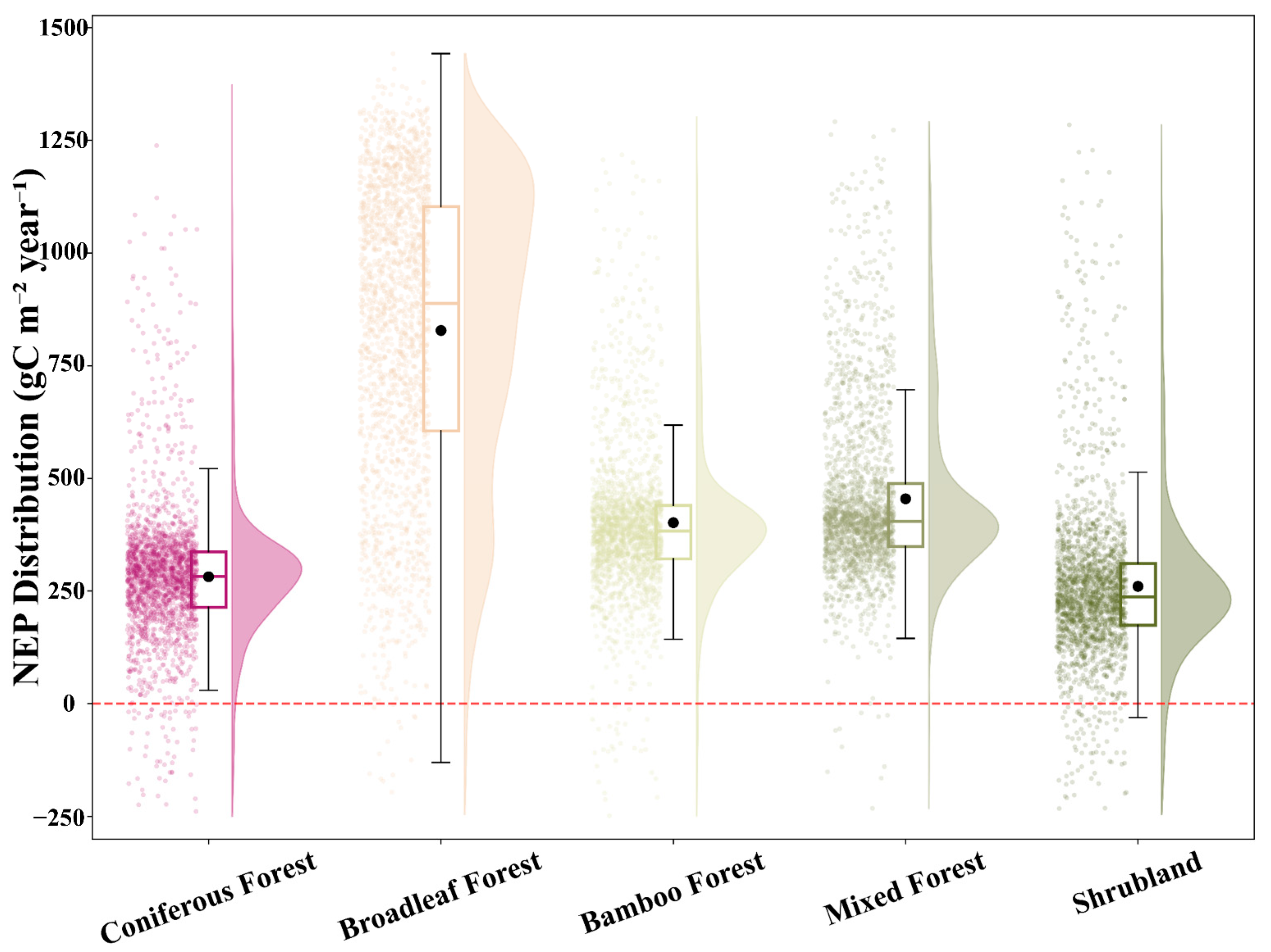
A comparison across vegetation types showed clear differences in forest NEP distribution (Figure 5). The mean NEP decreased in the order of broadleaf forest, mixed forest, bamboo forest, shrubland, and coniferous forest. Broadleaf forest had the highest mean and median NEP values, indicating the strongest net carbon uptake among the vegetation types. For all vegetation types, NEP showed long-tailed distributions and wide value ranges. This pattern indicates that NEP varied considerably within each vegetation type across the study area.

3.3. Spatial Autocorrelation Results

Spatial dependence of forest NEP was examined using spatial autocorrelation analysis. The Global Moran’s I value was 0.6752, which was significant at the 0.01 level. This indicates that forest NEP was not randomly distributed in space. Instead, areas with similar NEP values tended to cluster together, especially high-value areas.

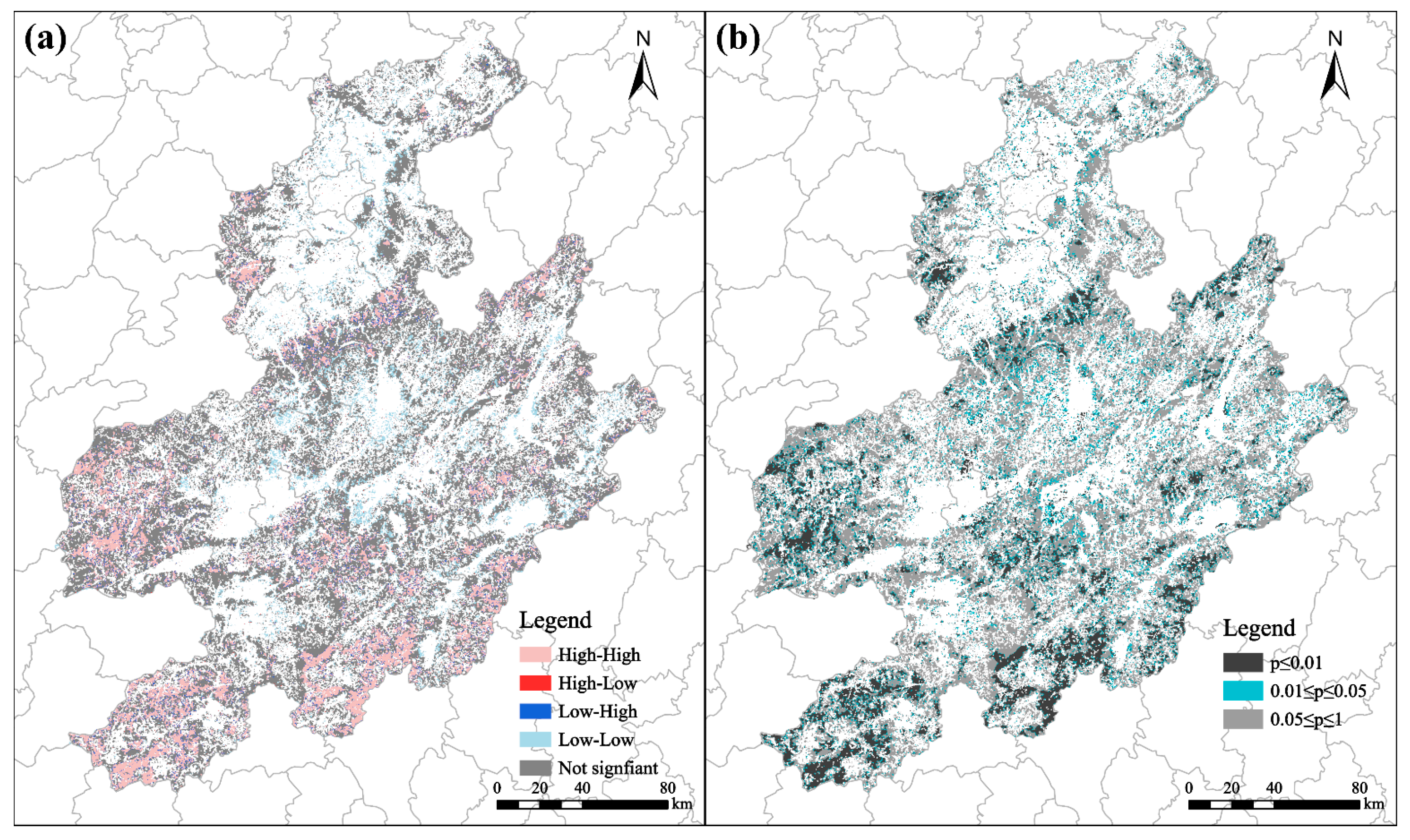
The LISA cluster map (Figure 6a) illustrates the local clustering patterns of NEP. High–High (HH) clusters covered 18.33% of the study area. These clusters were mainly distributed in peripheral mountainous regions, including the Luoxiao Mountains in the southwest, the southern parts of the Nanling Mountains, and the eastern marginal mountain areas. Low–Low (LL) clusters accounted for 10.52% within the study region. They were mainly distributed in the valley plains along the main channel of the Ganjiang River and in the central part of the Jitai Basin, including Jizhou District and Ji’an County.

The significance map showed that most HH and LL clusters overlapped with areas passing the 0.01 significance level (Figure 6b). This overlap indicates that the main clustering pattern was statistically reliable. Overall, the LISA results support the spatial pattern described above, with forest NEP exhibiting higher values in surrounding mountainous areas and lower values in central river valley regions.

3.4. Driving Factor Analysis of Forest NEP in the Middle and Upper Reaches of the Ganjiang River Basin

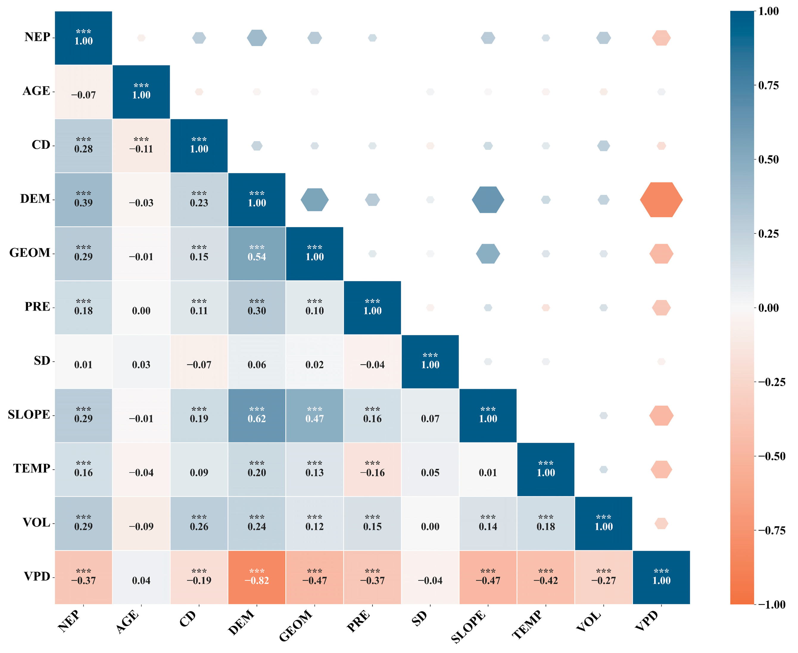
The selection of explanatory factors was based on the environmental conditions of the watershed and variables commonly used in related studies [54,55,56]. This study selected 10 potential explanatory factors, including DEM, SLOPE, and TEMP. Before correlation and model analysis, multicollinearity among these variables was tested. The VIF values of all variables were lower than five (Table S1), suggesting that strong collinearity was not present and that the selected variables were suitable for further analysis. Pearson correlation analysis was then used to provide a preliminary assessment of the relationships among variables. As shown in Figure 7, forest NEP was related to stand structure, terrain, and climate. Among the selected factors, VOL, CD, and DEM showed positive relationships with NEP, whereas VPD showed a negative relationship.

3.5. Analysis of Driving Forces for Forest NEP in the Middle and Upper Reaches of the Ganjiang River Based on SHAP

3.5.1. Model Performance Comparison and Selection

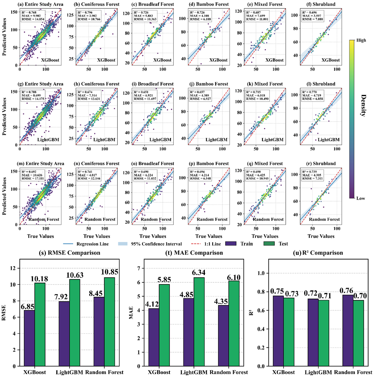
The analysis was carried out in Python 3.13. Three machine-learning models, namely Random Forest, LightGBM, and XGBoost, were used to describe the relationship between forest NEP and its potential driving factors, including hydroclimatic variables, biophysical attributes, and topographic factors. The dataset was randomly partitioned into training and testing sets in an 8:2 ratio. Bayesian optimization and five-fold cross-validation were then used during model training. The model performance is shown in Figure 8.

Random Forest and LightGBM showed similar fitting performance, achieving test R² values of 0.70 and 0.71, respectively. XGBoost achieved slightly higher performance than both models. It obtained the highest test ${\mathrm{R}}^2$ value of 0.73, together with the lowest MAE of 4.12 and RMSE of 6.85. The training and testing ${\mathrm{R}}^2$values were close to each other, at 0.75 and 0.73, respectively. This result indicates that the model had acceptable generalization performance and did not show significant overfitting. Therefore, XGBoost was selected as the basis for the following SHAP analysis. In this study, the model was used to support the interpretation of NEP driving factors rather than to generate NEP estimates.

3.5.2. Local Feature Model

A SHAP force plot for a sample point randomly selected from the study area is shown in Figure 9. The red and blue arrows represent the positive and negative effects of the driving factors on forest NEP, respectively. The area occupied by each variable within the arrows indicates the magnitude of its influence on NEP. DEM, SD and SLOPE were identified as the primary factors affecting NEP. Among them, DEM and SD exert positive effects on forest NEP, with the magnitude of their positive contributions decreasing sequentially. For this sample point, the SLOPE value is 3.26, which falls within a relatively low threshold range, thereby exerting a negative local effect on NEP.

3.5.3. Analysis of Factor Importance and Effect on Forest NEP

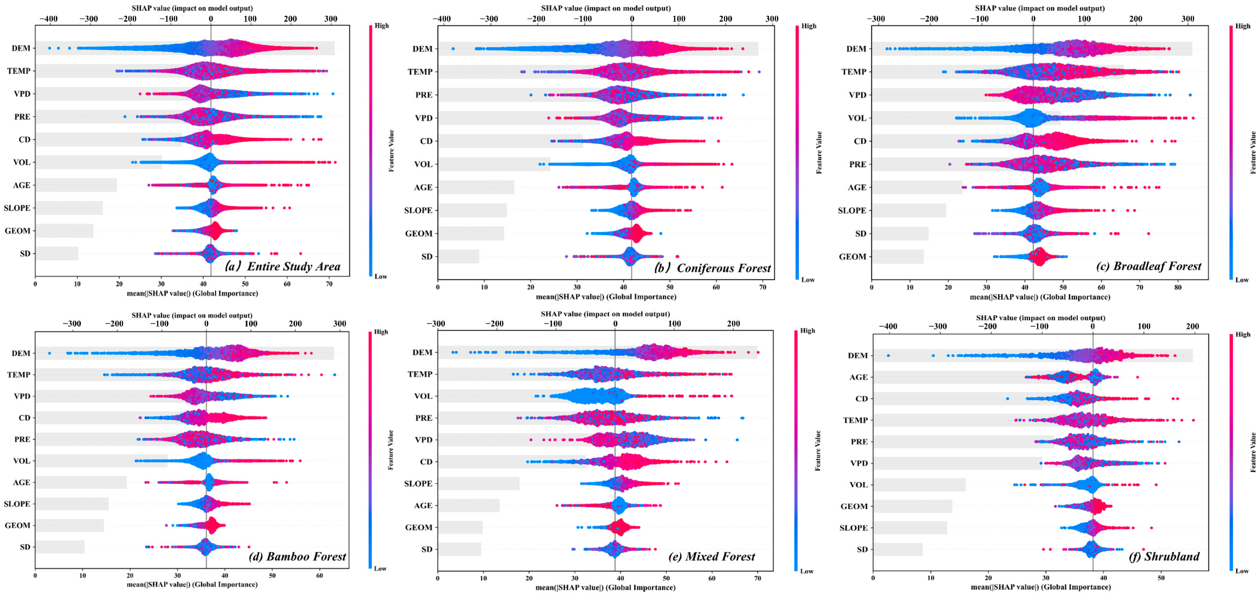
Forest NEP was influenced by topographic, climatic, and stand structural factors. To compare the roles of these variables, SHAP values were calculated based on the selected XGBoost model. The SHAP summary plots were used to show the relative importance of each factor and the direction of its effect on the model output (Figure 10).

At the regional scale, DEM, TEMP, and VPD were the three most important variables (Figure 10a). Higher DEM and TEMP values were mainly associated with positive SHAP values, suggesting that they tended to increase the NEP estimated by the model. For VPD, lower values were more often linked with positive SHAP values. This result indicates that a lower atmospheric moisture deficit was more favorable for forest NEP.

The main drivers differed among vegetation types. In coniferous, broadleaf, and bamboo forests, DEM and TEMP remained important factors, and a moisture-related variable, either PRE or VPD, also ranked highly (Figure 10b–d). This pattern suggests that these three vegetation types were mainly affected by topography and hydrothermal conditions. In mixed forests, DEM, TEMP, and VOL were the leading variables (Figure 10e). Higher VOL values generally contributed positively to NEP. In shrublands, DEM, AGE, and CD became the dominant factors, while the importance of TEMP and PRE decreased (Figure 10f). This result suggests that stand structure had a stronger effect on shrubland NEP than climatic factors.

3.5.4. Nonlinear Responses of Forest NEP to Key Driving Factors

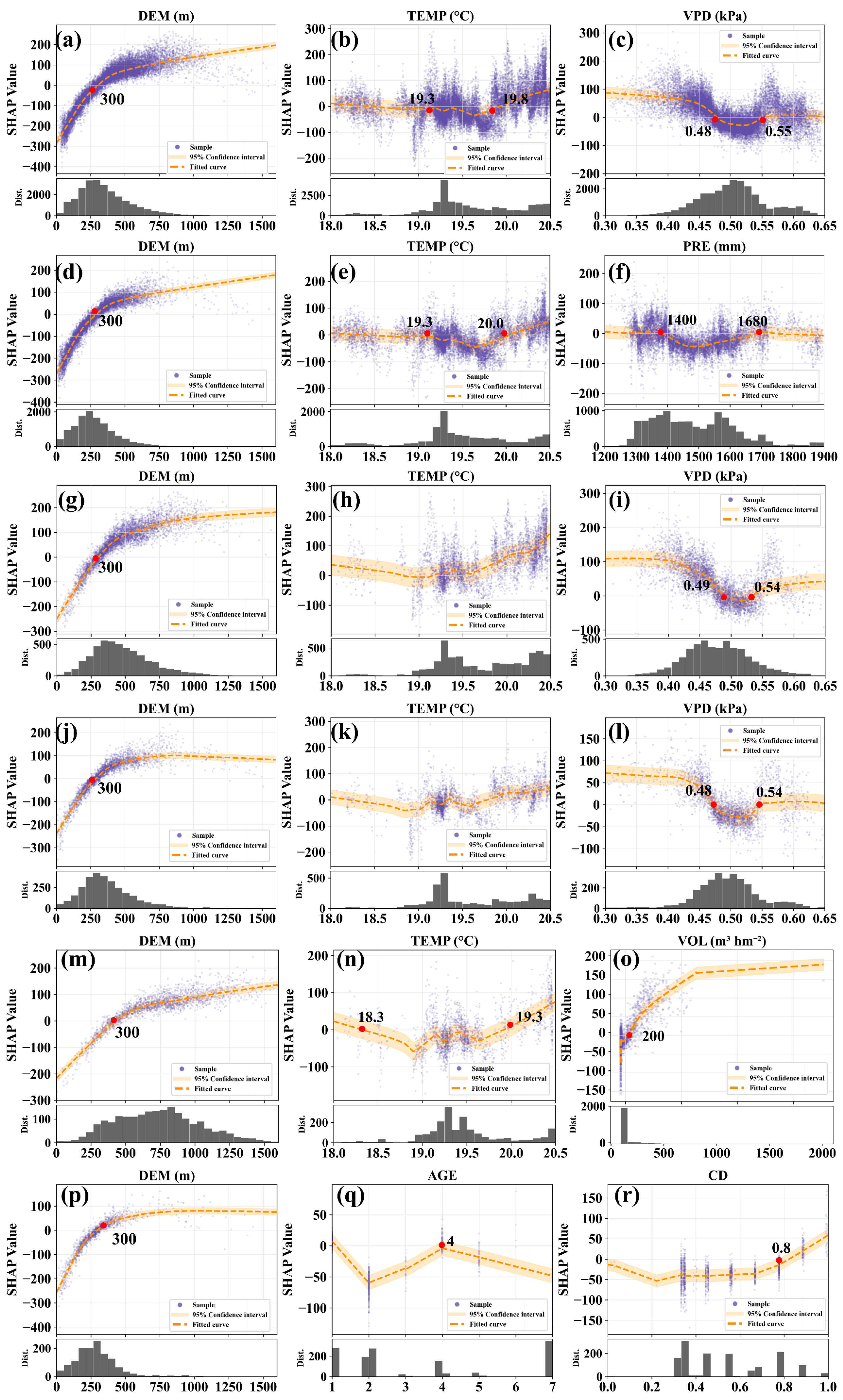
After the main variables were identified, SHAP dependence plots were used to examine the response patterns of forest NEP to these factors. Positive SHAP values indicate positive contributions to the NEP estimated by the model, whereas negative values indicate negative contributions to the model output. Figure 11 shows the SHAP dependence plots of the top three variables ranked by SHAP importance for the whole study area and each vegetation type. Figure 11 shows the dependence plots of the three main variables for the whole study area and each vegetation type.

For the whole study area, DEM showed a clear threshold response (Figure 11a–c). When elevation was below about 300 m, DEM mainly had negative SHAP values. Above this level, its effect became positive and then gradually stabilized. TEMP and VPD also showed nonlinear responses. TEMP had negative SHAP values mainly within 19.3–19.8 °C, while VPD showed negative values within 0.48–0.55 kPa. These ranges indicate conditions under which the NEP estimated by the model tended to decrease.

A similar elevation response was observed in coniferous forests (Figure 11d–f). DEM began to contribute positively when elevation exceeded about 300 m. PRE also showed a threshold pattern, with negative contributions mainly occurring within 1400–1680 mm.

For broadleaf forests, VPD showed a clear negative response in the SHAP results (Figure 11g–i). Its negative contributions were mainly concentrated within 0.49–0.54 kPa. Bamboo forests showed a similar VPD response range, approximately 0.48–0.54 kPa (Figure 11j–l). This pattern suggests that both broadleaf and bamboo forests were sensitive to atmospheric moisture deficit. In bamboo forests, the positive effect of elevation became weaker at higher altitudes.

In mixed forests, the response pattern was more closely related to stand structure (Figure 11m–o). VOL contributed positively to NEP when it was below approximately 200 m³ hm⁻². Beyond this level, the positive effect of VOL became weaker and gradually stabilized. This pattern suggests that the additional NEP gain from increasing stand volume may slow after a certain stage of stand development.

4. Discussion

4.1. Differential Drivers and Threshold Responses of NEP Among Vegetation Types

The SHAP results indicate that forest NEP in the middle and upper reaches of the Ganjiang River Basin is regulated by multiple interacting factors rather than a single environmental control. Its driving mechanisms varied among forest types and were jointly shaped by moisture availability, topographic conditions, and stand structure.

In coniferous forests, precipitation showed a clear nonlinear effect. Negative SHAP values mainly appeared within 1400–1680 mm. This pattern indicates that relatively high precipitation did not always increase NEP. One possible explanation is that excessive rainfall may reduce soil aeration and limit photosynthetically active radiation under frequent cloudy conditions [57,58,59]. Therefore, precipitation may have both positive and negative effects on forest NEP in humid subtropical regions.

Broadleaf and bamboo forests showed a different response. In these two vegetation types, VPD played a more important role than precipitation. Negative SHAP values were mainly concentrated within 0.48–0.54 kPa. This suggests that moderate atmospheric dryness may reduce NEP through stomatal regulation of photosynthesis [60]. The similar VPD range in broadleaf and bamboo forests also indicates a shared moisture constraint. In bamboo forests, the positive effect of elevation became weaker at higher altitudes. This pattern may reflect a narrower environmental adaptation range.

Mixed forests and shrublands were more strongly affected by stand structural factors. In mixed forests, VOL had a positive effect on NEP when it was below about 200 m³ hm⁻². After this level, the positive effect became weaker. This pattern suggests that the additional NEP gain from increasing stand volume may slow as stand development and biomass accumulation continue [61]. Therefore, forest management should not only focus on increasing stand volume after a relatively high level is reached. Stand structure, stand age, site conditions, and management goals should also be considered. In shrublands, CD showed a clear structural response. When CD exceeded 0.8, its positive effect on NEP became stronger. This result suggests that higher canopy closure and a more stable community structure may help improve NEP in shrublands [62]. Therefore, shrubland management should avoid excessive canopy reduction so that the community structure and understory microenvironment can remain relatively stable.

Overall, the main controls on NEP differed among vegetation types. Coniferous forests were mainly affected by precipitation. Broadleaf and bamboo forests were more sensitive to VPD. Mixed forests and shrublands were more closely related to stand structure. These differences indicate that regional carbon sink management should consider vegetation types rather than using a uniform strategy.

4.2. Interaction Effects of Driving Factors and Mechanisms Underlying Forest-Type Differentiation

Although the threshold response patterns provide useful insights, single-factor responses alone cannot fully explain differences in NEP among forest types. Because environmental variables operate interactively, their combined effects may further shape nonlinear NEP responses. This section, therefore, explores key driver interactions to better understand the mechanisms underlying forest-type differentiation.

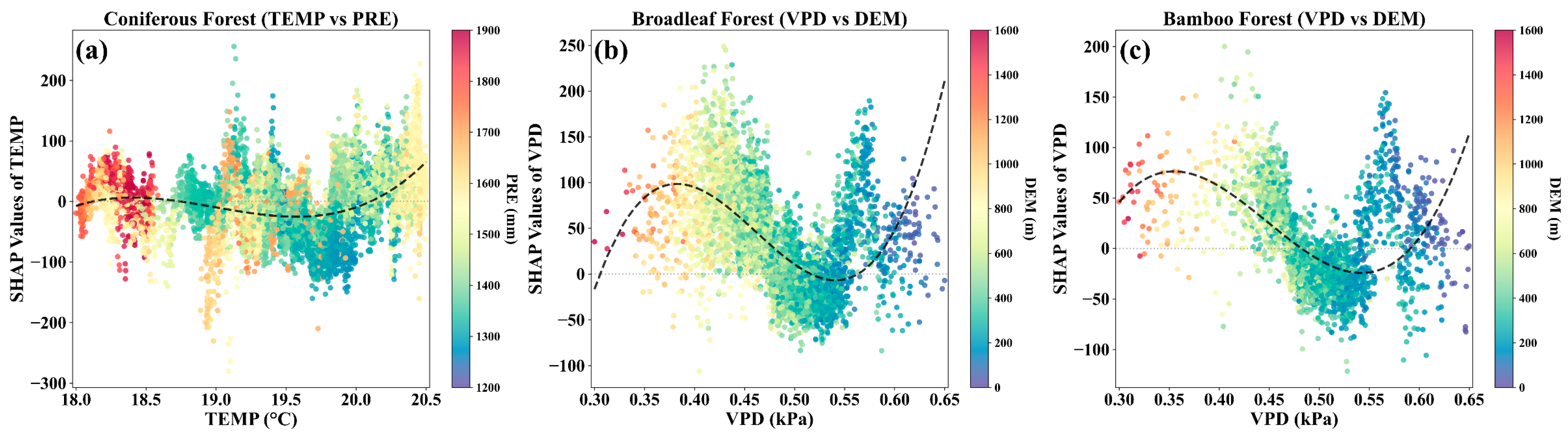
In coniferous forests, precipitation and temperature showed a clear interaction (Figure 12a). High precipitation values were mostly linked with lower temperature conditions. Under these conditions, temperature had a weak or slightly positive effect on NEP. By contrast, negative temperature effects mainly appeared under intermediate to high temperature conditions, and they were often linked with relatively lower precipitation. This pattern suggests that precipitation effects on NEP were modulated by hydro-thermal conditions. Precipitation did not act alone. Temperature and precipitation may jointly affect NEP through water availability, soil aeration, and radiation conditions [63].

Broadleaf and bamboo forests showed coupled effects between VPD and DEM (Figure 12b,c). Both vegetation types had a similar VPD threshold, approximately 0.48–0.54 kPa. However, the strength of the VPD effect changed with elevation. At lower elevations, VPD had a stronger negative effect on NEP. At higher elevations, this negative effect became weaker. This relationship indicates that elevation may moderate the effect of VPD [64]. Bamboo forests also showed a stronger decline in NEP under higher VPD and weaker recovery afterward. This response suggests that bamboo forests may be more sensitive to atmospheric dryness [65].

Together, these results show that differences in NEP among vegetation types were related not only to individual factors, but also to interactions among key drivers [66].

4.3. Limitations and Future Perspectives

The XGBoost–SHAP framework helped identify important variables and threshold responses of forest NEP. However, the interpretation of these results still has several limitations.

First, machine-learning models mainly describe relationships from data. They can capture complex nonlinear patterns, but they cannot fully represent all ecological and physical processes. XGBoost also has a black-box nature, although SHAP improves the interpretability of its outputs. Therefore, the attribution results should be understood as model-based explanations rather than direct causal evidence. Their reliability still depends on variable selection, data quality, and model structure [67].

Second, the validation of NEP estimates remains limited. This study evaluated CASA-simulated NPP using the MOD17A3HGF product. The estimated NEP was also compared with values reported in previous studies. These comparisons support the reliability of the results to some extent, but they cannot replace direct validation. Flux tower observations, forest inventory data, and field carbon flux measurements would help improve the accuracy of NEP estimation. Future studies should include more ground-based observations when such data are available.

Furthermore, the current study is inherently constrained by its spatial and temporal scope. Spatially, the analysis is confined to the middle and upper reaches of the Ganjiang River Basin. Temporally, the models were trained on a single-year snapshot of data from 2023, which is insufficient to comprehensively capture the interannual variability and long-term dynamic evolution of NEP. Future research extending this analytical framework to other geographical regions with diverse ecological conditions, while incorporating long-term time-series datasets, is highly warranted. Such efforts would profoundly enrich our understanding of the evolving trends and environmental response mechanisms across broader spatiotemporal scales [68,69,70,71].

5. Conclusions

This study estimated forest NEP in the middle and upper reaches of the Ganjiang River Basin for 2023. The spatial pattern of NEP and its driving factors were then analyzed using the XGBoost–SHAP framework. The main conclusions are as follows.

(1)

Forest NEP showed clear spatial distribution characteristics in the study area. Higher values were mainly found in the surrounding mountainous regions, while lower values appeared in the central river valleys. The Global Moran’s I value reached 0.6752, showing a significant positive spatial autocorrelation. This result means that forest NEP had a clear spatial clustering pattern. High–High (HH) clusters formed belt-like spatial patterns across the southwestern Luoxiao Mountains, the southern Nanling regions, and the eastern marginal mountain areas. Low–Low (LL) clusters mainly occurred in the Ganjiang River valley plain and the central Jitai Basin. The spatial distribution of forest NEP was closely related to local terrain conditions and forest structure.

(2)

At the regional scale, DEM, TEMP, and VPD were the most important factors associated with forest NEP. These results indicate that topography, thermal conditions, and atmospheric moisture conditions played important roles in NEP variation. The XGBoost–SHAP framework further identified the relative contributions of these factors and characterized their nonlinear responses.

(3)

The main drivers of NEP differed among vegetation types. Coniferous forests were mainly associated with precipitation. Broadleaf and bamboo forests were more sensitive to atmospheric moisture deficit. Mixed forests and shrublands were more strongly associated with stand structural variables, such as VOL, AGE, and CD. PRE within 1400–1680 mm and VPD within approximately 0.48–0.54 kPa showed negative contributions to the NEP estimated by the model. VOL and CD also showed threshold responses related to stand development and community structure.

(4)

Regional carbon sink management should consider differences among vegetation types. Coniferous, broadleaf, and bamboo forests responded differently to moisture-related factors, while mixed forests and shrublands were more closely linked to stand structure. Therefore, management strategies should be adjusted according to the dominant factors and threshold characteristics of each vegetation type.

References

1. Core Writing Team; Lee, H.; Romero, J. (Eds.) IPCC Climate Change 2023: Synthesis Report. Contribution of Working Groups I, II and III to the Sixth Assessment Report of the Intergovernmental Panel on Climate Change; Intergovernmental Panel on Climate Change (IPCC): Geneva, Switzerland, 2023. [Google Scholar]
2. Feng, H.; Kang, P.; Deng, Z.; Zhao, W.; Hua, M.; Zhu, X.; Wang, Z. The Impact of Climate Change and Human Activities to Vegetation Carbon Sequestration Variation in Sichuan and Chongqing. Environ. Res. 2023, 238, 117138. [Google Scholar] [CrossRef]
3. Piao, S.; Yue, C.; Ding, J.; Guo, Z. Perspectives on the Role of Terrestrial Ecosystems in the ‘Carbon Neutrality’ Strategy. Sci. China Earth Sci. 2022, 65, 1178–1186. [Google Scholar] [CrossRef]
4. Mo, L.; Zohner, C.M.; Reich, P.B.; Liang, J.; De Miguel, S.; Nabuurs, G.-J.; Renner, S.S.; Van Den Hoogen, J.; Araza, A.; Herold, M.; et al. Integrated Global Assessment of the Natural Forest Carbon Potential. Nature 2023, 624, 92–101. [Google Scholar] [CrossRef]
5. Friedlingstein, P.; Sitch, S.; O’Sullivan, M. China’s Land Carbon Budget in the Context of the Global Carbon Budget. Natl. Sci. Rev. 2025, 12, nwaf073. [Google Scholar] [CrossRef] [PubMed]
6. Zhao, J.; Liu, D.; Zhu, Y.; Peng, H.; Xie, H. A Review of Forest Carbon Cycle Models on Spatiotemporal Scales. J. Clean. Prod. 2022, 339, 130692. [Google Scholar] [CrossRef]
7. Piao, S.; He, Y.; Wang, X.; Chen, F. Estimation of China’s Terrestrial Ecosystem Carbon Sink: Methods, Progress and Prospects. Sci. China Earth Sci. 2022, 65, 641–651. [Google Scholar] [CrossRef]
8. Yang, Y.; Shi, Y.; Sun, W.; Chang, J.; Zhu, J.; Chen, L.; Wang, X.; Guo, Y.; Zhang, H.; Yu, L.; et al. Terrestrial Carbon Sinks in China and around the World and Their Contribution to Carbon Neutrality. Sci. China Life Sci. 2022, 65, 861–895. [Google Scholar] [CrossRef]
9. Liu, D.; Zhang, Z.; Liu, Z.; Chi, Y. A Three-Class Carbon Pool System for Normalizing Carbon Mapping and Accounting in Coastal Areas. Ecol. Indic. 2024, 158, 111537. [Google Scholar] [CrossRef]
10. Zhong, J.; Zhang, X.; Guo, L.; Wang, D.; Miao, C.; Zhang, X. Ongoing CO2 Monitoring Verify CO2 Emissions and Sinks in China during 2018–2021. Sci. Bull. 2023, 68, 2467–2476. [Google Scholar] [CrossRef]
11. Yao, Y.; Li, Z.; Wang, T.; Chen, A.; Wang, X.; Du, M.; Jia, G.; Li, Y.; Li, H.; Luo, W.; et al. A New Estimation of China’s Net Ecosystem Productivity Based on Eddy Covariance Measurements and a Model Tree Ensemble Approach. Agric. For. Meteorol. 2018, 253–254, 84–93. [Google Scholar] [CrossRef]
12. Zhang, M.; He, H.; Zhang, L.; Yu, G.; Ren, X.; Lv, Y.; Niu, Z.; Qin, K.; Gao, Y. Increased Ecological Land and Atmospheric CO2 Dominate the Growth of Ecosystem Carbon Sinks under the Regulation of Environmental Conditions in National Key Ecological Function Zones in China. J. Environ. Manag. 2024, 366, 121906. [Google Scholar] [CrossRef] [PubMed]
13. Xu, W.; Cheng, Y.; Luo, M.; Mai, X.; Wang, W.; Zhang, W.; Wang, Y. Progress and Limitations in Forest Carbon Stock Estimation Using Remote Sensing Technologies: A Comprehensive Review. Forests 2025, 16, 449. [Google Scholar] [CrossRef]
14. Potter, C.; Pass, S. Changes in the Net Primary Production of Ecosystems across Western Europe from 2015 to 2022 in Response to Historic Drought Events. Carbon Balance Manag. 2024, 19, 32. [Google Scholar] [CrossRef]
15. Zhang, Y.; Shao, Z.; Xu, X.; Zhuang, Q. Quantifying Urban Vegetation Carbon Storage Using Seamless and Dense Time-Series Remote Sensing Data. Geo-Spat. Inf. Sci. 2025, 28, 1–19. [Google Scholar] [CrossRef]
16. Lu, X.; Chen, Y.; Sun, Y.; Xu, Y.; Xin, Y.; Mo, Y. Spatial and Temporal Variations of Net Ecosystem Productivity in Xinjiang Autonomous Region, China Based on Remote Sensing. Front. Plant Sci. 2023, 14, 1146388. [Google Scholar] [CrossRef] [PubMed]
17. Ji, S.; Ren, S.; Fang, L.; Chen, J.; Wang, G.; Wang, Q. Improved CASA-Based Net Ecosystem Productivity Estimation in China by Incorporating Developmental Factors into Autumn Phenology Model. Remote Sens. 2025, 17, 487. [Google Scholar] [CrossRef]
18. Han, J.; Meng, X.; Lin, L.; Lu, J. Spatial and Temporal Patterns of Vegetation Carbon Sources/Sinks and Driving Factors in Southeastern Xizang from 2000 to 2020. PeerJ 2026, 14, e20572. [Google Scholar] [CrossRef]
19. Thölix, L.; Backman, L.; Havu, M.; Karvinen, E.; Soininen, J.; Trémeau, J.; Nevalainen, O.; Ahongshangbam, J.; Järvi, L.; Kulmala, L. Carbon Sequestration in Different Urban Vegetation Types in Southern Finland. Biogeosciences 2025, 22, 725–749. [Google Scholar] [CrossRef]
20. Li, Y.; Li, J.; Tang, J.; Tan, J.; Ma, T.; Li, K. Dynamics and Driving Factors of Vegetation Carbon Sources and Sinks in Shanxi Province, China. Int. J. Environ. Sci. Technol. 2026, 23, 230. [Google Scholar] [CrossRef]
21. Su, R.; Guo, E.; Wu, L.; Wang, Y.; Li, X.; Wang, P.; Dai, L.; Sun, Z. Predicting Net Primary Productivity Response to Multiple Extreme Climate Drivers in Inner Mongolia. Environ. Res. Lett. 2026, 21, 014010. [Google Scholar] [CrossRef]
22. Li, X.; Huntingford, C.; Wang, K.; Cui, J.; Xu, H.; Kan, F.; Anniwaer, N.; Yang, H.; Penuelas, J.; Piao, S. Increased Crossing of Thermal Stress Thresholds of Vegetation under Global Warming. Glob. Change Biol. 2024, 30, e17406. [Google Scholar] [CrossRef]
23. Lau, M.S.Y.; Becker, A.; Madden, W.; Waller, L.A.; Metcalf, C.J.E.; Grenfell, B.T. Comparing and Linking Machine Learning and Semi-Mechanistic Models for the Predictability of Endemic Measles Dynamics. PLoS Comput. Biol. 2022, 18, e1010251. [Google Scholar] [CrossRef] [PubMed]
24. Menefee, D.; Lee, T.O.; Flynn, K.C.; Chen, J.; Abraha, M.; Baker, J.; Suyker, A. Machine Learning Algorithms Improve MODIS GPP Estimates in United States Croplands. Front. Remote Sens. 2023, 4, 1240895. [Google Scholar] [CrossRef]
25. Reichstein, M.; Camps-Valls, G.; Stevens, B.; Jung, M.; Denzler, J.; Carvalhais, N. Prabhat Deep Learning and Process Understanding for Data-Driven Earth System Science. Nature 2019, 566, 195–204. [Google Scholar] [CrossRef] [PubMed]
26. Han, B.A.; Varshney, K.R.; LaDeau, S.; Subramaniam, A.; Weathers, K.C.; Zwart, J. A Synergistic Future for AI and Ecology. Proc. Natl. Acad. Sci. USA 2023, 120, e2220283120. [Google Scholar] [CrossRef]
27. Suleymanov, A.; Abakumov, E.; Savin, I. Explainable Data-Driven Spatial Predictions of Soil Organic Carbon at the National Level. Sci. Total Environ. 2026, 1013, 181291. [Google Scholar] [CrossRef] [PubMed]
28. Gao, P.; Mu, X.; Wang, F.; Li, R. The Response of Sediment Yield to Land Use and Climate Change in the Ganjiang River Basin, China. Catena 2021, 207, 105658. [Google Scholar] [CrossRef]
29. Liu, Y.; Shen, H.; Ge, G.; Xing, A.; Tang, Z.; Fang, J. Classification and Distribution of Evergreen Broad-Leaved Forests in Jiangxi, East China. J. Plant Ecol. 2023, 16, rtac059. [Google Scholar] [CrossRef]
30. Zhou, C.; Cheng, W.; Qian, J. Geomorphological Atlas of the People’s Republic of China (1:1,000,000); Science Press: Beijing, China, 2009. [Google Scholar]
31. Potter, C.S.; Randerson, J.T.; Field, C.B.; Matson, P.A.; Vitousek, P.M.; Mooney, H.A.; Klooster, S.A. Terrestrial Ecosystem Production: A Process Model Based on Global Satellite and Surface Data. Glob. Biogeochem. Cycles 1993, 7, 811–841. [Google Scholar] [CrossRef]
32. Papaioannou, G.; Papanikolaou, N.; Retalis, D. Relationships of Photosynthetically Active Radiation and Shortwave Irradiance. Theor. Appl. Climatol. 1993, 48, 23–27. [Google Scholar] [CrossRef]
33. Szeicz, G. Solar Radiation for Plant Growth. J. Appl. Ecol. 1974, 11, 617–636. [Google Scholar] [CrossRef]
34. Zhu, W.; Pan, Y.; He, H.; Yu, D.; Hu, H. Simulation of Maximum Light Use Efficiency for Some Typical Vegetation Types in China. Chin. Sci. Bull. 2006, 51, 457–463. [Google Scholar] [CrossRef]
35. Huang, C.; Sun, C.; Nguyen, M.; Wu, Q.; He, C.; Yang, H.; Tu, P.; Hong, S. Spatio-Temporal Dynamics of Terrestrial Net Ecosystem Productivity in the ASEAN from 2001 to 2020 Based on Remote Sensing and Improved CASA Model. Ecol. Indic. 2023, 154, 110920. [Google Scholar] [CrossRef]
36. Zhiyong, P.; Hua, O.; Caiping, Z.; Xingliang, X. CO2 Processes in an Alpine Grassland Ecosystem on the Tibetan Plateau. J. Geogr. Sci. 2003, 13, 429–437. [Google Scholar] [CrossRef]
37. Chen, D.; Zhang, C.; Wu, J.; Zhou, L.; Lin, Y.; Fu, S. Subtropical Plantations Are Large Carbon Sinks: Evidence from Two Monoculture Plantations in South China. Agric. For. Meteorol. 2011, 151, 1214–1225. [Google Scholar] [CrossRef]
38. Yan, F.; Wang, M.; Shan, J.; Ding, Y.; Dong, L.; Zhang, Y.; Zhang, H.; Xu, H.; Pang, J.; Chen, Y. An Integrated Social-Ecological Indicator for Low-Carbon Transition: Evidence from the Beijing-Tianjin-Hebei, China. Ecol. Indic. 2025, 175, 113553. [Google Scholar] [CrossRef]
39. Lai, J.; Qi, S.; Chen, J.; Guo, J.; Wu, H.; Chen, Y. Exploring the Spatiotemporal Variation of Carbon Storage on Hainan Island and Its Driving Factors: Insights from InVEST, FLUS Models, and Machine Learning. Ecol. Indic. 2025, 172, 113236. [Google Scholar] [CrossRef]
40. Xiang, Q.; Wei, R.; Qin, C.; Fu, L.; Li, Z.; He, H.; Shu, Q. Forest Aboveground Carbon Storage in the Three Parallel Rivers Region: A Remote Sensing and Machine Learning Perspective. Remote Sens. 2026, 18, 756. [Google Scholar] [CrossRef]
41. Wang, X.; Wang, Y.; Song, L.; Dai, S.; Zang, C. Analysis of Interrelated Characteristics between Ecosystem Services and Ecosystem Health in the Guangdong–Hong Kong–Macao Greater Bay Area. Front. Plant Sci. 2025, 16, 1668073. [Google Scholar] [CrossRef]
42. Song, Z.; Shi, P.; Li, P.; Li, Z.; Niu, H.; Zu, P.; Cao, M.; Jia, Y. Effects of Forest Type on Carbon Storage in the Hilly Region of Loess Plateau, China. Front. For. Glob. Change 2024, 7, 1349047. [Google Scholar] [CrossRef]
43. Wang, T.; Dong, L.; Liu, Z. Factors Driving Carbon Accumulation in Forest Biomass and Soil Organic Carbon across Natural Forests and Planted Forests in China. Front. For. Glob. Change 2024, 6, 1333868. [Google Scholar] [CrossRef]
44. Pan, S.; Liu, Z.; Han, Y.; Zhang, D.; Zhao, X.; Li, J.; Wang, K. Using the Pearson’s Correlation Coefficient as the Sole Metric to Measure the Accuracy of Quantitative Trait Prediction: Is It Sufficient? Front. Plant Sci. 2024, 15, 1480463. [Google Scholar] [CrossRef] [PubMed]
45. Lv, Q.; Yang, H.; Wang, J.; Feng, G.; Liu, W.; Zhang, Y.; Wang, W.; Wang, C.; Huang, X.; Cui, L.; et al. Estimating Regional Terrestrial Ecosystem Carbon Sinks on Multi-Model Coupling Approach. Ecol. Indic. 2025, 178, 114041. [Google Scholar] [CrossRef]
46. Cai, Y.; Zhu, P.; Li, X.; Liu, X.; Chen, Y.; Shen, Q.; Xu, X.; Zhang, H.; Nie, S.; Wang, C.; et al. Dynamics of China’s Forest Carbon Storage: The First 30 m Annual Aboveground Biomass Mapping from 1985 to 2023. Earth Syst. Sci. Data 2025, 17, 6993–7018. [Google Scholar] [CrossRef]
47. Zheng, M.; Wen, Q.; Xu, F.; Wu, D. Regional Forest Carbon Stock Estimation Based on Multi-Source Data and Machine Learning Algorithms. Forests 2025, 16, 420. [Google Scholar] [CrossRef]
48. Song, J.; Liu, X.; Adingo, S.; Guo, Y.; Li, Q. A Comparative Analysis of Remote Sensing Estimation of Aboveground Biomass in Boreal Forests Using Machine Learning Modeling and Environmental Data. Sustainability 2024, 16, 7232. [Google Scholar] [CrossRef]
49. Dhawi, F.; Ghafoor, A.; Almousa, N.; Ali, S.; Alqanbar, S. Predictive Modelling Employing Machine Learning, Convolutional Neural Networks (CNNs), and Smartphone RGB Images for Non-Destructive Biomass Estimation of Pearl Millet (Pennisetum glaucum). Front. Plant Sci. 2025, 16, 1594728. [Google Scholar] [CrossRef] [PubMed]
50. Sharma, P.; Sahoo, B.B. Precise Prediction of Performance and Emission of a Waste Derived Biogas–Biodiesel Powered Dual–Fuel Engine Using Modern Ensemble Boosted Regression Tree: A Critique to Artificial Neural Network. Fuel 2022, 321, 124131. [Google Scholar] [CrossRef]
51. Sharma, P.; Sahoo, B.B. An ANFIS-RSM Based Modeling and Multi-Objective Optimization of Syngas Powered Dual-Fuel Engine. Int. J. Hydrogen Energy 2022, 47, 19298–19318. [Google Scholar] [CrossRef]
52. Wen, Z.; Zhou, Z.; Wei, X.; Xiao, D.; Xu, L.; Wan, W. Spatio-Temporal Simulation of the Productivity of Four Typical Subtropical Forests: A Case Study of the Ganjiang River Basin in China. Forests 2025, 16, 603. [Google Scholar] [CrossRef]
53. Zheng, J.; Mao, F.; Du, H.; Li, X.; Zhou, G.; Dong, L.; Zhang, M.; Han, N.; Liu, T.; Xing, L. Spatiotemporal Simulation of Net Ecosystem Productivity and Its Response to Climate Change in Subtropical Forests. Forests 2019, 10, 708. [Google Scholar] [CrossRef]
54. Xu, X.; Zhang, X.; Qin, L.; Li, R. Unveiling Spatiotemporal Evolution and Driving Factors of Ecosystem Service Value: Interpretable HGB-SHAP Machine Learning Model. Front. Environ. Sci. 2025, 13, 1640840. [Google Scholar] [CrossRef]
55. Feng, K.; Yuan, H.; Li, Y.; Wang, Y.; Su, X.; Huang, S.; Wang, F.; Zhang, Z. Three-Dimensional Analysis of Carbon Source Events in the Yellow River Basin: Lifecycles, Triggers, and Linkages to Long-Term Trend Mutations. Ecol. Indic. 2025, 181, 114471. [Google Scholar] [CrossRef]
56. Song, X.; Chen, X.; Zheng, B.; Wan, W. Spatiotemporal Patterns and Driving Mechanisms of Terrestrial Carbon Sinks in Jiangxi Province, Subtropical China. Carbon Balance Manag. 2026, 21, 60. [Google Scholar] [CrossRef]
57. Ren, S.; Xu, X.; Jia, G.; Artaxo, P.; Machado, L.A.T.; Montes, J.A.G.; Nobre, C.A.; Rizzo, L.; Xiao, X. Excessive Wetness Suppresses Carbon Sink of Amazon Forest Under Seasonal Water Surplus. Glob. Change Biol. 2025, 31, e70422. [Google Scholar] [CrossRef] [PubMed]
58. Yang, X.; Yang, K.; Zhang, S.; Zeng, W.; Liu, J.; Rao, Y.; Ma, Y.; Bi, C. Precipitation Dominates Forest Net Primary Productivity Variations with Distinct Regional Differences in Yunnan Province, China. Ecol. Evol. 2026, 16, e72893. [Google Scholar] [CrossRef] [PubMed]
59. Mo, J.; Yan, H.; Hu, B.; Chen, C.; Zhou, X.; Chen, Y. Spatial and Temporal Dynamics and Climate Contribution of Forest Ecosystem Carbon Sinks in Guangxi During 2000–2023. Forests 2026, 17, 151. [Google Scholar] [CrossRef]
60. Li, W.; Yue, F.; Wang, C.; Liao, J.; Zhang, X. Climatic Influences on Intra-Annual Stem Variation of Larix Principis-Rupprechtii in a Semi-Arid Region. Front. For. Glob. Change 2022, 5, 948022. [Google Scholar] [CrossRef]
61. Zhu, K.; Zhang, J.; Niu, S.; Chu, C.; Luo, Y. Limits to Growth of Forest Biomass Carbon Sink under Climate Change. Nat. Commun. 2018, 9, 2709. [Google Scholar] [CrossRef] [PubMed]
62. Li, Y.; Guo, J.; Guo, Y.; Chai, Y.; Yue, M. Shrubland Carbon Storage in Northern China: A Synergistic Analysis of Climate, Plant Community and Soil Traits. J. Plant Ecol. 2025, 18, rtaf097. [Google Scholar] [CrossRef]
63. Ploschuk, R.A.; Savin, R.; Slafer, G.A. Dual Stress, Equivalent Harm? Hypothesizing on the Type of Interactions between Waterlogging and High Temperature. Front. Plant Sci. 2025, 15, 1472665. [Google Scholar] [CrossRef]
64. Johnston, M.R.; Barnes, M.L.; Preisler, Y.; Smith, W.K.; Biederman, J.A.; Scott, R.L.; Williams, A.P.; Dannenberg, M.P. Effects of Hot Versus Dry Vapor Pressure Deficit on Ecosystem Carbon and Water Fluxes. J. Geophys. Res. Biogeosci. 2025, 130, e2024JG008146. [Google Scholar] [CrossRef]
65. Michaud, J.M.; Mocko, K.; Schenk, H.J. Positive Pressure in Bamboo Is Generated in Stems and Rhizomes, Not in Roots. AoB Plants 2024, 16, plae040. [Google Scholar] [CrossRef]
66. Zou, Y.; Wang, X. Analysis of Influencing Factors of Terrestrial Carbon Sinks in China Based on LightGBM Model and Bayesian Optimization Algorithm. Sustainability 2025, 17, 4836. [Google Scholar] [CrossRef]
67. Naser, M.Z. Fundamental Flaws of Physics-Informed Neural Networks and Explainability Methods in Engineering Systems. Comput. Ind. Eng. 2026, 212, 111704. [Google Scholar] [CrossRef]
68. Besnard, S.; Koirala, S.; Santoro, M.; Weber, U.; Nelson, J.; Gütter, J.; Herault, B.; Kassi, J.; N’Guessan, A.; Neigh, C.; et al. Mapping Global Forest Age from Forest Inventories, Biomass and Climate Data. Earth Syst. Sci. Data 2021, 13, 4881–4896. [Google Scholar] [CrossRef]
69. Vega García, M.; Aznarte, J.L. Shapley Additive Explanations for NO2 Forecasting. Ecol. Inform. 2020, 56, 101039. [Google Scholar] [CrossRef]
70. Silva, S.J.; Keller, C.A.; Hardin, J. Using an Explainable Machine Learning Approach to Characterize Earth System Model Errors: Application of SHAP Analysis to Modeling Lightning Flash Occurrence. J. Adv. Model. Earth Syst. 2022, 14, e2021MS002881. [Google Scholar] [CrossRef]
71. Wang, J.; Shao, Z.; Fu, P.; Zhuang, Q.; Chang, J.; Jing, P.; Zhao, Z.; Xu, Z.; Wang, S.; Yang, F. Unraveling the Impact of Urban Expansion on Vegetation Carbon Sequestration Capacity: A Case Study of the Yangtze River Economic Belt. Sustain. Cities Soc. 2025, 120, 106157. [Google Scholar] [CrossRef]
Figure 1. Geographic location of the middle and upper reaches of the Ganjiang River Basin.
Forests 17 00651 g001
Figure 2. Workflow for estimating forest NEP and analyzing its driving factors.
Forests 17 00651 g002
Figure 3. Accuracy verification of CASA model-simulated NPP against MODIS product.
Forests 17 00651 g003
Figure 4. Spatial pattern of forest NEP in the middle and upper reaches of the Ganjiang River Basin in 2023.
Forests 17 00651 g004
Figure 5. Differences in forest NEP distribution among vegetation types.
Forests 17 00651 g005
Figure 6. Spatial clustering pattern and statistical significance of forest NEP in the middle and upper reaches of the Ganjiang River Basin in 2023. (a) Local Indicators of Spatial Association (LISA) cluster map showing High–High (HH) and Low–Low (LL) clusters. (b) Spatial distribution of statistical significance (p-value) for the LISA clustering results.
Forests 17 00651 g006
Figure 7. Heatmap of Pearson correlation coefficients among variables. *** indicates significance at p < 0.001.
Forests 17 00651 g007
Figure 8. Performance comparison of XGBoost, LightGBM, and Random Forest in fitting the relationship between forest NEP and driving factors. Panels (ar) show the fitted relationships between observed and model-estimated NEP for each model and vegetation type, and panels (su) compare model performance using RMSE, MAE, and R 2 .
Forests 17 00651 g008
Figure 9. SHAP force plot of individual sample analysis.
Forests 17 00651 g009
Figure 10. SHAP plots of driving factors for forest NEP across the entire study area and each vegetation type. Panels (af) represent the entire study area, coniferous forest, broadleaf forest, bamboo forest, mixed forest, and shrubland, respectively. (a) Entire study area SHAP summary plot, (b) coniferous forest SHAP summary plot, (c) broadleaf forest SHAP summary plot, (d) bamboo forest SHAP summary plot, (e) mixed forest SHAP summary plot, and (f) shrubland SHAP summary plot.
Forests 17 00651 g010
Figure 11. SHAP dependence plots of key driving factors for forest NEP. Panels (ac) show DEM, TEMP, and VPD for the whole study area; panels (df) show DEM, TEMP, and PRE for coniferous forest; panels (gi) show DEM, TEMP, and VPD for broadleaf forest; panels (jl) show DEM, TEMP, and VPD for bamboo forest; panels (mo) show DEM, AGE, and VOL for mixed forest; and panels (pr) show DEM, AGE, and CD for shrubland.
Forests 17 00651 g011
Figure 12. SHAP interaction plots of key driving factors for forest NEP. (a) TEMP–PRE interaction in coniferous forest; (b) VPD–DEM interaction in broadleaf forest; (c) VPD–DEM interaction in bamboo forest.
Forests 17 00651 g012