Article

Forest Fire Risk Early Warning Based on Dynamic Fuel Moisture Content

by
Yuanzong Li
,
Cui Zhou
*,
Junxiang Zhang
,
Wenjun Wang
,
Zhenyu Chen
and
Yongfeng Luo
School of Advanced Interdisciplinary Studies, Central South University of Forestry and Technology, Changsha 410004, China
*
Author to whom correspondence should be addressed.
Forests 2026, 17(5), 532; https://doi.org/10.3390/f17050532
Submission received: 25 March 2026 / Revised: 16 April 2026 / Accepted: 24 April 2026 / Published: 28 April 2026

Abstract

Accurate prediction of forest fires is crucial for enhancing regional fire prevention and control. Existing models frequently rely on static factors such as weather and terrain, while insufficiently taking into account the Fuel Moisture Content (FMC), a critical internal factor that directly determines fire behavior. Instead, proxies like the Normalized Difference Vegetation Index (NDVI) are commonly employed, which weakens the physical foundation of predictions. This study assesses the marginal contribution of integrating dynamic FMC into fire prediction models. Concentrating on California, we developed a random-forest-based model that incorporates high-resolution FMC products retrieved by our team, along with meteorological, topographic, vegetation, and anthropogenic data. Through comparative experiments and SHapley Additive exPlanations (SHAP) analysis, we evaluated model improvements and the contribution mechanisms of key drivers. The results indicated that: (1) Incorporating FMC significantly enhanced model performance, with precision and specificity increasing by 3.93% and 3.60%, respectively, and the Area Under the Curve (AUC) showing improvements, suggesting heightened sensitivity in detecting actual fire occurrences. (2) SHAP analysis disclosed nonlinear effects and threshold dynamics: temperature was the dominant positive driver (the fire risk soared above 20 °C); FMC demonstrated a negative correlation with fire risk, with 100% serving as a potential threshold; elevation presented an inverted U-shaped pattern (the peak risk occurred at 1000–1500 m); and population density exhibited a shifting influence from positive to negative. (3) The monthly risk maps for California in 2023 captured the seasonal progression of fire risk and spatial patterns consistent with historical fire points. The fire risk map for 9 September 2020 also demonstrated consistency with the spatial distribution of the actual fire points on that day. This study validates that the integration of dynamic FMC strengthens the mechanistic foundation and early-warning capacity of fire prediction models, providing scientific backing for targeted fire management.

1. Introduction

In the context of global climate change, the frequency and intensity of forest fires have increased significantly [1,2,3], posing serious threats to ecosystem security, sustainable socio-economic development, and human life and property. According to statistics, millions of hectares of forest are burned globally each year, releasing substantial amounts of greenhouse gases and causing irreversible ecological damage [4]. In this situation, developing scientific and effective fire prediction models has become a crucial approach to enhancing fire prevention and control capabilities and optimizing the allocation of fire management resources [5,6,7,8,9,10]. The core of fire prediction is to establish quantitative relationships between the probability of fire occurrence and multi-source explanatory variables. Through integrated analyses of meteorological conditions, topographic features, vegetation status, and human activities, dynamic fire risk prediction and spatial expression can be achieved, providing a scientific basis for targeted fire prevention [11,12,13,14,15].
Throughout the development process of fire prediction models, research methodologies have experienced a systematic evolution from traditional statistical models to modern artificial-intelligence-based approaches [15,16,17,18,19]. In the early stages of research, conventional regression models such as linear regression and logistic regression, along with bivariate statistical methods including frequency ratio and weight of evidence, were predominantly employed. For example, Bian et al. [20] carried out a comprehensive analysis of the spatiotemporal distribution of forest fires in Zhejiang Province from 2013 to 2023. They used eight contributing factors as indicator variables to develop logistic regression (LR), random forest, and gradient-boosting models, among which the latter two exhibited better predictive capabilities. Gao et al. [21] made use of meteorological data, topographic data, and historical fire records to predict forest fires in the Heihe region of Heilongjiang Province based on random forest and back-propagation neural networks. Li et al. [22] extracted potential driving factors, namely meteorological conditions, slope, and normalized difference vegetation index, to identify the determinants of fire occurrence. They constructed forest fire prediction models using machine learning algorithms and concluded that the random forest model achieved the highest accuracy. Lee et al. [23] integrated human proximity variables, surface fuel load, and meteorological data to develop an ensemble approach that improved the accuracy of fire risk prediction.
The studies suggest that forest fire risk prediction methodologies are evolving from single-model statistical approaches to multi-source data fusion, from static prediction to dynamic early warning, and from traditional methods to intelligent algorithms. Nevertheless, existing research has mainly concentrated on external driving factors such as meteorology, topography, vegetation indices, and human activities, while inadequate attention has been given to FMC, a critical internal factor that directly determines fire behavior. Current studies generally use NDVI as a substitute for FMC. As a core parameter characterizing fuel combustibility, FMC directly controls ignition probability, rate of spread, and fire intensity, acting as a crucial link between environmental conditions and fire behavior [24,25,26]. However, the acquisition of FMC data has long been restricted by the limitations of traditional observation methods [27]. Although field sampling surveys can offer local accuracy, they are time-consuming and labor-intensive, making it challenging to meet the spatiotemporal continuity requirements for large-scale, multi-temporal fire risk prediction [27,28,29]. Owing to these constraints, most regional-scale fire prediction models have been forced to use proxy indicators such as the Normalized Difference Vegetation Index to indirectly characterize fuel status, which, to some degree, undermines the physical basis and predictive potential of these models. In recent years, with the rapid development of remote sensing retrieval technologies, especially the emergence of multi-source remote sensing collaborative inversion frameworks, dynamic, high-precision, and spatiotemporally continuous FMC products have gradually become achievable. This progress provides crucial data support for overcoming traditional data limitations and directly integrating FMC, this core driving factor, into fire prediction modeling frameworks.
Based on the aforementioned analysis, this study devises a multi-source data-driven fire prediction model that integrates FMC, with the random forest algorithm serving as the core methodology. It systematically explores the contribution of FMC to the prediction accuracy of the model. Random forest, being a typical ensemble learning algorithm, demonstrates strong nonlinear fitting capabilities, resistance to overfitting, and functions for evaluating variable importance, which allows for the effective management of complex relationships among multi-source heterogeneous data. By comparing the performance of the model with and without the incorporation of FMC factors, this study intends to verify the role of FMC in fire prediction, present scientific evidence for the development of more physically based high-precision fire prediction models, and thereby offer technical support for targeted regional fire prevention and control.

2. Materials

2.1. Test Site

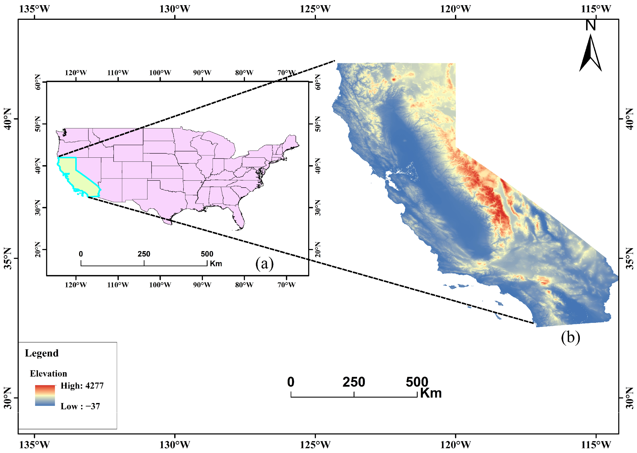
The study area is situated in California, United States, covering latitudes ranging from 32° N to 42° N and longitudes from 114° W to 124° W (Figure 1), with an approximate total area of 424,000 km2. The terrain is characterized by complexity and diversity, incorporating major geographic entities such as the Coast Ranges, the Sierra Nevada, and the Central Valley. The predominant vegetation types are shrublands and coniferous forests, which offer ample fuel conditions for the occurrence of forest fires. The region demonstrates distinct Mediterranean-climate characteristics, marked by hot and dry summers and mild and wet winters. Moreover, the frequent incidence of strong foehn winds, such as the Santa Ana winds in autumn, significantly heightens the potential for the rapid spread of fires, making California one of the global hotspots for forest fires. Additionally, as urban development continues to encroach upon wildland–urban interface areas, the interaction between human activities and natural ecosystems further intensifies the complexity and uncertainty of fire risk. Consequently, this study chose California as the experimental area for forest-fire risk prediction, comprehensively analyzing the spatial patterns of fire risk under the combined influence of multiple factors, including meteorology, topography, vegetation, and human activities, with the aim of providing scientific support for fire prevention and emergency management in this region.

2.2. Data

2.2.1. FMC Data

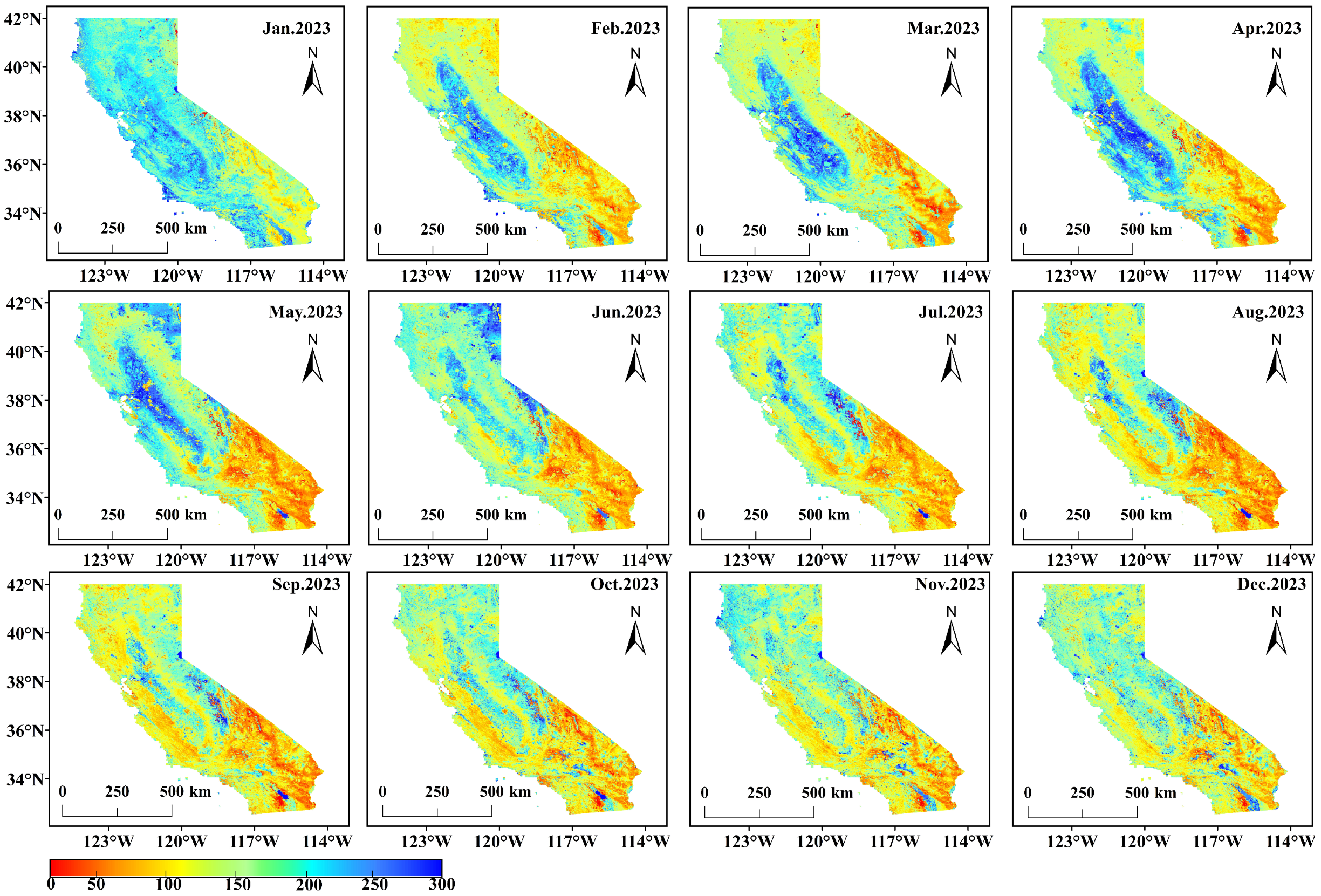
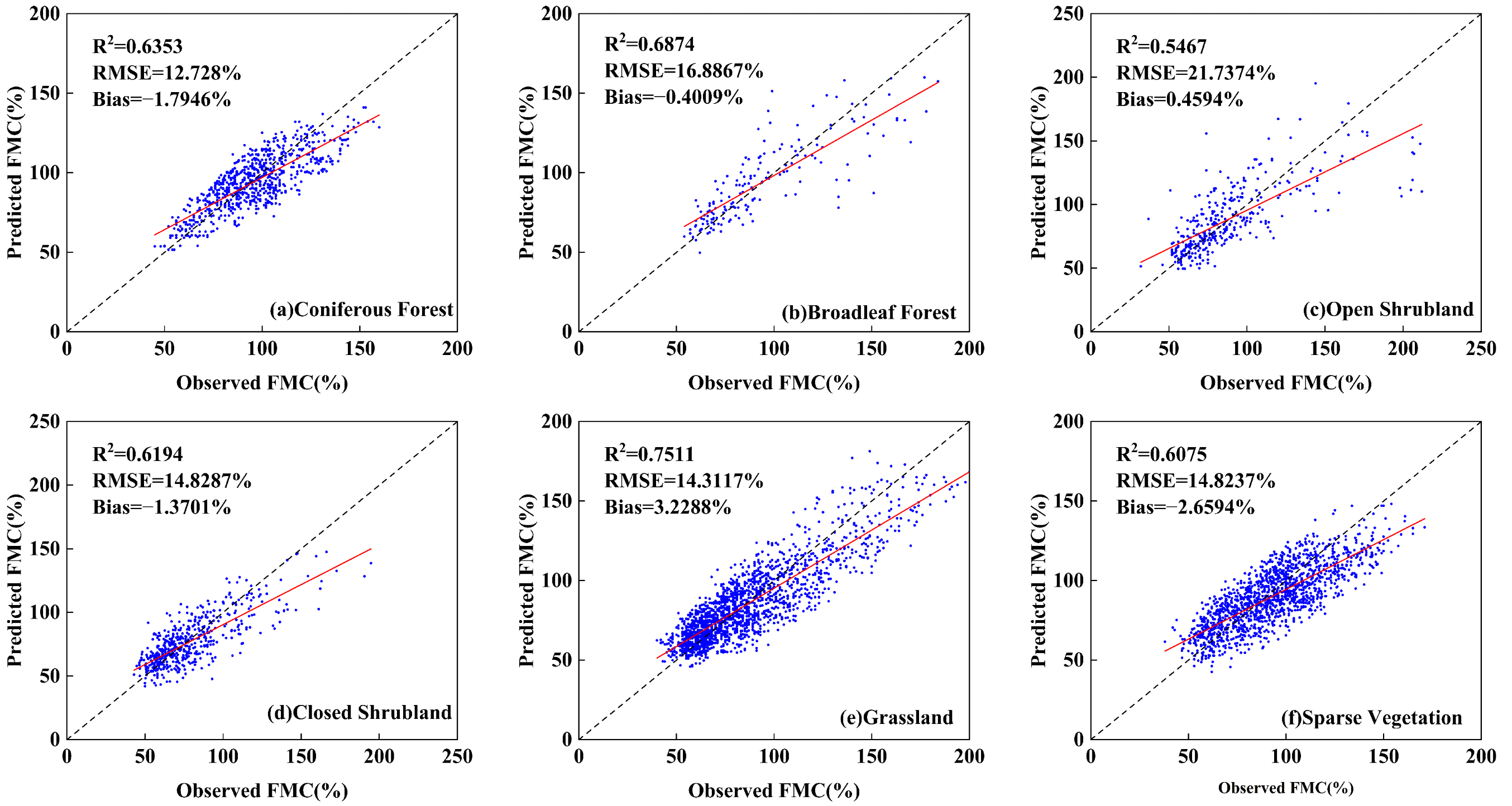
The FMC serves as a critical indicator for forecasting the risk of forest fires. The FMC data utilized in this study were derived from the previously developed NRCBLA framework, and the figure depicts the monthly average data for 2023 (Figure 2). The ground-measured data employed in this study were acquired from the U.S. National Fuel Moisture Database. The input variables of the NRCBLA algorithm encompass seven spectral bands from MCD43A4, five meteorological factors from ERA5 (U/V wind speed, 2-m temperature, evapotranspiration, and vegetation interception), and two topographic parameters from SRTM (elevation and slope). All variables were uniformly resampled to a spatial resolution of 500 m. The training data consisted of 19,236 ground-measured samples collected throughout California from 2015 to 2023, which were partitioned into a training set and an independent test set at a ratio of 7:3. The model adopted a vegetation-type-specific modeling approach. Based on the IGBP classification system, vegetation was re-categorized into six types: coniferous forest, broadleaf forest, closed shrubland, open shrubland, grassland, and sparse vegetation. Independent CBLA models were trained for each type. The CBLA model architecture sequentially consists of: a CNN module (with 3 × 3 convolutional kernels and 2 × 2 max pooling layers) to extract spatial features, a BiLSTM module to capture bidirectional temporal dependencies, and an Attention module to dynamically weight key features. Model hyperparameter optimization was carried out using the Newton–Raphson-based optimizer (NRBO) for adaptive adjustment, with a search agent number of 6 and a maximum iteration number of 5, using the minimization of mean squared error as the fitness function, ultimately yielding the FMC predictions. This framework was employed to generate daily, spatiotemporally continuous FMC data that covered the study area from 2020 to 2023. The accuracy of FMC was assessed using metrics such as the coefficient of determination (R2), root mean square error (RMSE), and bias. As depicted in Table 1, the scatter plot of the predicted values against the NFMD ground-measured values is presented in Figure 3.

2.2.2. Vegetation Data

The Normalized Difference Vegetation Index (NDVI) stands as one of the most widely utilized indicators that reflect vegetation growth vitality, coverage density, and greenness. High values of NDVI generally correspond to dense vegetation, while low values indicate bare soil or water bodies. The NDVI data employed in this study were sourced from the product MCD43A Version 6.1 (MCD43A4.061) [30,31]. The MCD43A4 product offers daily surface reflectance data corrected by the Bidirectional Reflectance Distribution Function (BRDF), which effectively mitigates the influence of angular effects on vegetation monitoring. The dataset employed in this research spans the period from 1 January 2020 to 31 December 2023, featuring a daily temporal resolution. The NDVI extracted from this product precisely captures vegetation coverage and phenological changes in the study area. It serves as a crucial indicator for characterizing fuel load and dryness conditions and is directly integrated into the spatial prediction of fire risk.

2.2.3. Meteorological and Topographic Data

The auxiliary data for this study consist of two components: topography and meteorology. Topographic data were obtained from the SRTM digital elevation model (DEM) to extract elevation, slope, and aspect [32], which allows for the characterization of terrain controls on vegetation distribution and fuel dryness conditions. Regarding meteorological data, only the ERA5 daily mean temperature was chosen, excluding other variables such as precipitation and relative humidity [33]. The reasoning behind this selection is two-fold: dynamic FMC data themselves represent the integrated response to multiple meteorological factors, and their variations have already incorporated critical meteorological information. Incorporating additional meteorological variables would potentially lead to information redundancy and multicollinearity problems. Therefore, only temperature was introduced as an auxiliary variable representing thermal conditions to ensure the parsimony and robustness of the fire risk prediction model.

2.2.4. Anthropogenic Factors Data

To quantify the influence of human activities on forest fire risk, this study selected two types of anthropogenic variables: population density and road networks. The population density data were obtained from the LandScan Global 2022 dataset developed by Oak Ridge National Laboratory [34,35]. This dataset goes beyond the traditional assumption of uniform population distribution within administrative units. It integrates multi-source data, such as nighttime lights, land use, roads, and topography, to construct a residential suitability model. Subsequently, it allocates national census data to approximately 1 km grid cells with higher precision, offering reliable support for revealing the influence of human settlement intensity on ignition probability.
Road network data were acquired from the “World Roads” (2023) basemap service on the Esri ArcGIS(10.8) platform, which incorporates global major highways, roads of diverse classifications, and ferry routes. These data not only function as a direct indicator of the accessibility of human activities but also serve as a fundamental geospatial framework for analyzing the spatial pathways of human-induced ignitions and evaluating the accessibility for fire suppression endeavors. The data were utilized in line with Esri’s licensing agreement, solely for mapping and spatial analysis purposes within this study.

2.2.5. Fire Occurrence Data

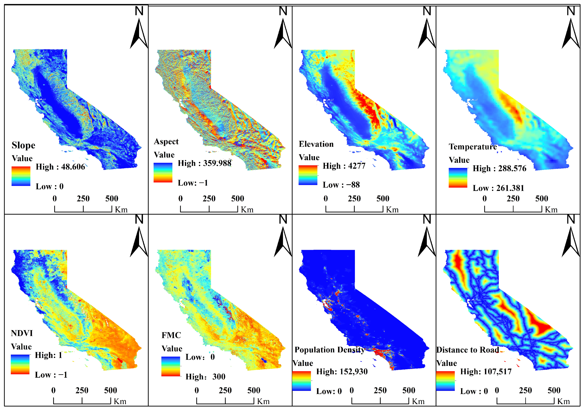
The fire occurrence data utilized in this study were sourced from the MODIS MCD64A1 (Version 6.1) monthly burned area product [36]. The dataset utilized in this study spans the period from January 2020 to December 2023, featuring a monthly temporal resolution and encompassing a total of 48 scenes. This product documents global burned pixels and their corresponding burn dates (encoded in Julian days) at a spatial resolution of 500 m, relying on surface reflectance observations and a dynamic threshold algorithm. In this study, pixels with a burn date greater than zero were recognized as valid fire points and served as true labels for the training samples of the model. These fire points were spatially and temporally matched with multi-source data, encompassing meteorological, topographic, vegetation, and anthropogenic variables, to establish a machine-learning sample set for fire risk prediction. The forest fire driving factors taken into account in the model are presented in Table 2 and Figure 4.
To ensure the temporal alignment between fire occurrence and dynamic variables, this study employed a rigorous date-matching strategy. Based on the quality-control band provided by the MCD64A1 product, the burn-date data were filtered to retain only high-quality burned pixels. For each quality-controlled burned pixel, the burn date recorded in the product was regarded as the fire occurrence time. The FMC value, NDVI value, and daily average temperature of that pixel on the burn date were extracted and allocated to the corresponding fire sample. Static variables did not require temporal matching. The MCD64A1 product designates a single burn date to each burned pixel via a dynamic threshold algorithm, representing the estimated initial burn date. Therefore, there is no problem of ambiguity or multiple fire dates within the same period. This date-matching strategy ensures that the model learns the relationship between fuel moisture conditions and fire occurrence at the exact ignition time.
To guarantee rigorous spatial and temporal alignment of multi-source data and satisfy the input consistency requirements for forest fire risk prediction modeling, all dynamic data in this study were subjected to unified preprocessing. To address the data gaps and cloud contamination issues in NDVI and FMC, quality control and gap-filling procedures were carried out based on the MCD43A4 Version 6.1 (MCD43A4.061) product. Firstly, regarding the spatial scale, considering that the native spatial resolution of key dynamic data sources (such as FMC and NDVI retrieved from MODIS) is approximately 500 m, all raster data were uniformly resampled to a 500-m spatial resolution to preserve the textural details of the original information and minimize errors caused by scale transformation. Bilinear interpolation was utilized during resampling to prevent significant distortion in the spatial statistical properties of continuous variables (e.g., temperature, population density). Secondly, in the temporal dimension, to capture the dynamic characteristics of fire risk over short timescales, all dynamic variables involved in risk prediction (including FMC, NDVI, and daily mean temperature) were uniformly stored and processed in a daily format, ensuring strict temporal alignment among factors. Missing values and masked pixels in NDVI and FMC were reconstructed through linear interpolation based on adjacent valid observations to guarantee temporal continuity. Topographic data (DEM and its derived slope and aspect) were regarded as static inputs and directly incorporated into modeling after spatial registration. Through the above-mentioned preprocessing workflow, a spatiotemporally consistent dataset with unified resolution was established, providing reliable data support for subsequent integrated fire risk prediction.
In the analysis of forest fire influencing factors, considering the varying dimensions and magnitudes among factors, directly utilizing the raw data for modeling would cause disproportionately high weights for factors with larger numerical values. This may overshadow the contributions of factors with smaller magnitudes and result in significant prediction errors. To eliminate the dimensional influences and magnitude differences and ensure that all features possess equal explanatory power in the model, this study conducted dimensionless processing on all continuous influencing factors. Specifically, the min–max normalization method was adopted to map the raw data of each factor to the [0, 1] interval via linear transformation [37]. The transformation function of this method is defined as follows:
x = x x m i n x m a x x m i n
where x represents the normalized dimensionless value, x m i n and x m a x respectively denote the minimum and maximum values of the factor within the sample set, and x is the original sample value of the influencing factor.

3. Methodology

3.1. Random Forest Model

This study utilizes the Random Forest ensemble learning algorithm to develop a forest fire risk prediction model. The objective is to combine the static environmental background with the dynamic Fuel Moisture Content (FMC) for a comprehensive risk assessment. The Random Forest algorithm, put forward by Breiman in 2001, is an ensemble learning approach based on the concepts of Bagging and random subspace. By constructing multiple decision trees and aggregating their classification outcomes, it presents several advantages, such as the efficient processing of high-dimensional data, the alleviation of overfitting, and the provision of feature importance interpretation [38,39,40]. The construction procedure of the Random Forest algorithm mainly comprises three steps. Firstly, the bootstrap sampling method is applied to randomly select samples with replacement from the original training set, generating bootstrap sample sets, each of which has the same size as the original training set. The samples that are not selected form the out-of-bag data, which can be used for an unbiased estimation of the model error. Secondly, a classification and regression tree is constructed for each bootstrap sample set. During the node splitting process in each tree, features are randomly chosen from the full feature set, and the optimal splitting feature and threshold are selected for partitioning. This random feature selection mechanism effectively reduces the correlation among trees and improves the generalization ability of the ensemble model. Finally, for new samples, each tree produces a classification result, and the final prediction of the Random Forest is determined through majority voting. Its mathematical representation is presented in Equation (2):
H ( x ) = m a j o r i t y   v o t e { h t ( x ) } t = 1 T
where H ( x ) is obtained through majority voting of the prediction results from all decision trees, T represents the total number of decision trees, and h t denotes the prediction output of the t-th decision tree for sample x .
In the process of model construction, the occurrence of forest fires was defined as a binary dependent variable. Specifically, when the predicted probability of fire occurrence exceeded 0.5, the location was classified as a fire-prone point (coded as 1); conversely, it was classified as a non-fire-prone point (coded as 0). This study designed a comparative experiment, in which two models were constructed: a baseline model that incorporated traditional static environmental factors (such as topography, vegetation, and human activities) and meteorological factors, and an integrated model that further included dynamic daily FMC features. Through a systematic comparison of the predictive performance of the two models, the critical value of dynamic FMC in forest fire risk prediction was empirically determined.
The model construction adhered to standard machine-learning procedures. Initially, historical fire point data were spatially matched with multi-dimensional driving factors to guarantee that each fire sample corresponded to a comprehensive set of feature variables. To address the issue of class imbalance (where fire samples are generally significantly fewer than non-fire samples), this study employed an environmental stratified random sampling strategy with the FMC as the stratifying variable. The FMC comprehensively reflects the moisture status of vegetation, integrating multiple types of environmental information including vegetation type, topography, and meteorology. It also serves as the most direct and core controlling factor for fire risk. Specifically, based on the physiological characteristics of vegetation moisture and the sample distribution, the FMC was classified into four levels: less than 50% (extremely dry), 50%–100% (dry), 100%–150% (moist), and greater than 150% (very moist). Within each FMC stratum, non-fire point samples were randomly selected from unburned pixels at a 1:1 ratio. In comparison with synthetic sampling techniques such as SMOTE, this strategy maintains the true spatial distribution characteristics of non-fire samples and ensures a consistent distribution of fire and non-fire points in terms of the core fuel moisture conditions, effectively preventing sampling bias.
Hyperparameters were pre-determined by taking into account computational efficiency and overfitting control. The number of decision trees was set at 100, which is a commonly used default value in random forests. This value strikes a reasonable balance between model performance and computational cost, as research has indicated that the improvement in performance tends to plateau when the number of trees exceeds 100. The minimum leaf size was set to 100 to control the depth of the trees and prevent overfitting. Considering the relatively large training sample size in this study, a larger minimum leaf size contributes to enhancing the model’s generalization ability. To ensure the rigor of the comparative experiment, both models employed the same parameter configuration. To further assess model stability and reduce the random bias resulting from a single spatial partition, 5-fold spatial cross-validation was applied to the training set. This study utilized a total of 47,618 samples, encompassing 47,274 distinct spatial locations, with over 99% of the locations having only one observation. The specific steps are as follows:
(1)
Spatial Stratified Sampling: The 33,092 distinct spatial locations within the training set were partitioned into five approximately equal subsets, with each subset containing roughly 6618 locations. A stratified sampling approach was employed to ensure that the proportion of positive and negative samples in each subset remained consistent with that of the original training set, thereby avoiding the influence of class imbalance on the validation results.
(2)
Iterative Validation Process: In each iteration, four subsets (approximately 26,474 locations) were chosen as the training set, while the remaining subset functioned as the validation data. This process was repeated five times, guaranteeing that each spatial location was utilized as the validation set precisely once.
(3)
Spatial Independence Assurance: Since the division unit is the spatial location rather than individual samples, all samples from the same location invariably belong to the same subset, ensuring complete spatial independence between the training and validation sets. In this dataset, each location has an average of merely 1.01 samples, leading to an extremely low risk of data leakage due to spatial autocorrelation. The implementation of a rigorous spatial block cross-validation strategy demonstrates methodological rigor.
All the above processing was performed in MATLAB (R2016a). After each iteration, the AUC, accuracy, precision, recall, specificity, and F1 score of the two models on the validation set were calculated. After aggregating the results of the five iterations, the values of each metric were determined. Upon the completion of 5-fold spatial cross-validation, the performance of the models was evaluated on a spatially independent test set, where there was no spatial overlap between the training set and the test set, thus ensuring the authenticity and reliability of the evaluation results. By comparing the performance disparities between the two models in cross-validation and on the independent test set, the marginal contribution of dynamic FMC to fire risk prediction was quantified.

3.2. Feature Importance Ranking Based on the SHAP Interpretation Framework

Feature importance pertains to a method for scoring the input features of a predictive model, which can disclose the relative contribution of each driving factor to fire assessment [41,42,43]. Traditional feature importance evaluation methods, such as those founded on Gini impurity or mean squared error reduction, generally depend on model internal mechanisms and are calculated based on the training set. When the model demonstrates overfitting, these importance measures may become skewed. Moreover, for deep-learning models with intricate internal structures, the nonlinear mapping relationships between inputs and outputs are challenging to interpret directly, rendering it infeasible to acquire reliable feature importance rankings through the model itself. To tackle these issues, this study presents the SHAP (SHapley Additive exPlanations) interpretability framework for model explainability analysis. The SHAP method, based on the Shapley value theory from cooperative game theory, computes the weighted average of each feature’s marginal contributions across all possible feature subsets, obtaining the SHAP value for that feature, thus equitably allocating each feature’s contribution to the prediction outcome [44,45,46]. SHAP values can uniformly represent both the direction and magnitude of feature contributions, where positive values signify positive driving effects, negative values signify negative driving effects, and their absolute values reflect contribution intensity. The SHAP value for a feature is defined in Equation (3):
φ j = 1 | N | S N l e f t { j } | S | ! ( | N | | S | 1 ) ! [ f ( S { j } ) f ( S ) ]
where N represents the set of all features, S denotes a feature subset derived from N subsequent to the removal of feature j , f ( S ) represents the model output based on the feature subset S , and f ( S { j } ) f ( S ) represents the marginal contribution of feature j under the current feature combination.
Based on the aforementioned theory, the specific implementation steps of the SHAP analysis in this research are as follows. Initially, all features were normalized to eliminate the impact of dimensionality. The mapminmax function was utilized to linearly map each feature to the [0, 1] interval. Subsequently, SHAP values were computed. This algorithm can precisely calculate the SHAP values of each feature and notably enhance computational efficiency. To avoid interpretation bias resulting from uneven sample partitioning, this research further put forward a segmented balanced sampling strategy: in accordance with the actual distribution range of each feature, it was divided into 5 to 6 continuous intervals, and an equal number of fire-point samples (approximately 83–100 per interval) were extracted from each interval. Approximately 500 analysis samples were independently constructed for each feature, ensuring that the SHAP analysis covered the entire range of feature values. On this foundation, this research adopted two SHAP visualization methods to improve model interpretability. The first is the SHAP summary plot, which presents feature importance, the direction of impact, and the distribution of SHAP values across the entire sample. The second is the SHAP dependence plot, which demonstrates the interaction between feature values and their SHAP values, facilitating the identification of the influence patterns of feature value changes on prediction results and key thresholds. These visualization analyses play a significant role in comprehending how each feature affects fire occurrence and identifying critical thresholds.

3.3. Performance Evaluation Metrics

To quantitatively assess the predictive performance of the Random Forest model for forest fire risk, a multi-dimensional accuracy evaluation framework was established to comprehensively reflect the classification effectiveness of the model from various statistical perspectives [47,48]. This framework consists of five core metrics: Accuracy gauges the overall correct classification rate of the model; Precision denotes the proportion of true fire points among samples predicted as fire points, emphasizing the reliability of prediction results; Recall reflects the proportion of actual fire points that are successfully recognized, indicating the model’s capacity to capture fire events; the F1 score, as the harmonic mean of Precision and Recall, offers a balanced and comprehensive consideration of both; the AUC value evaluates the model’s comprehensive discriminatory ability across different decision thresholds by computing the area under the ROC curve, remaining impervious to imbalanced class distributions. These metrics are computed based on the true positives, true negatives, false positives, and false negatives obtained from the confusion matrix, collectively establishing a quantitative basis for a comprehensive and objective comparison of the predictive performance between the baseline model and the integrated model. The specific formulas are as follows:
A c c u r a c y = T P + T N T P + T N + F P + F N
P r e c i s i o n = T P T P + F P
R e c a l l = T P T P + F N
F 1 = 2 × P r e c i s i o n × R e c a l l P r e c i s i o n + R e c a l l
S p e c i f i c i t y = T P T N + F P
where T P represents True Positives, T N represents True Negatives, F P represents False Positives, and F N represents False Negatives.

4. Results

4.1. Analysis and Interpretation of Forest Fire Risk Factors

4.1.1. Correlation Analysis

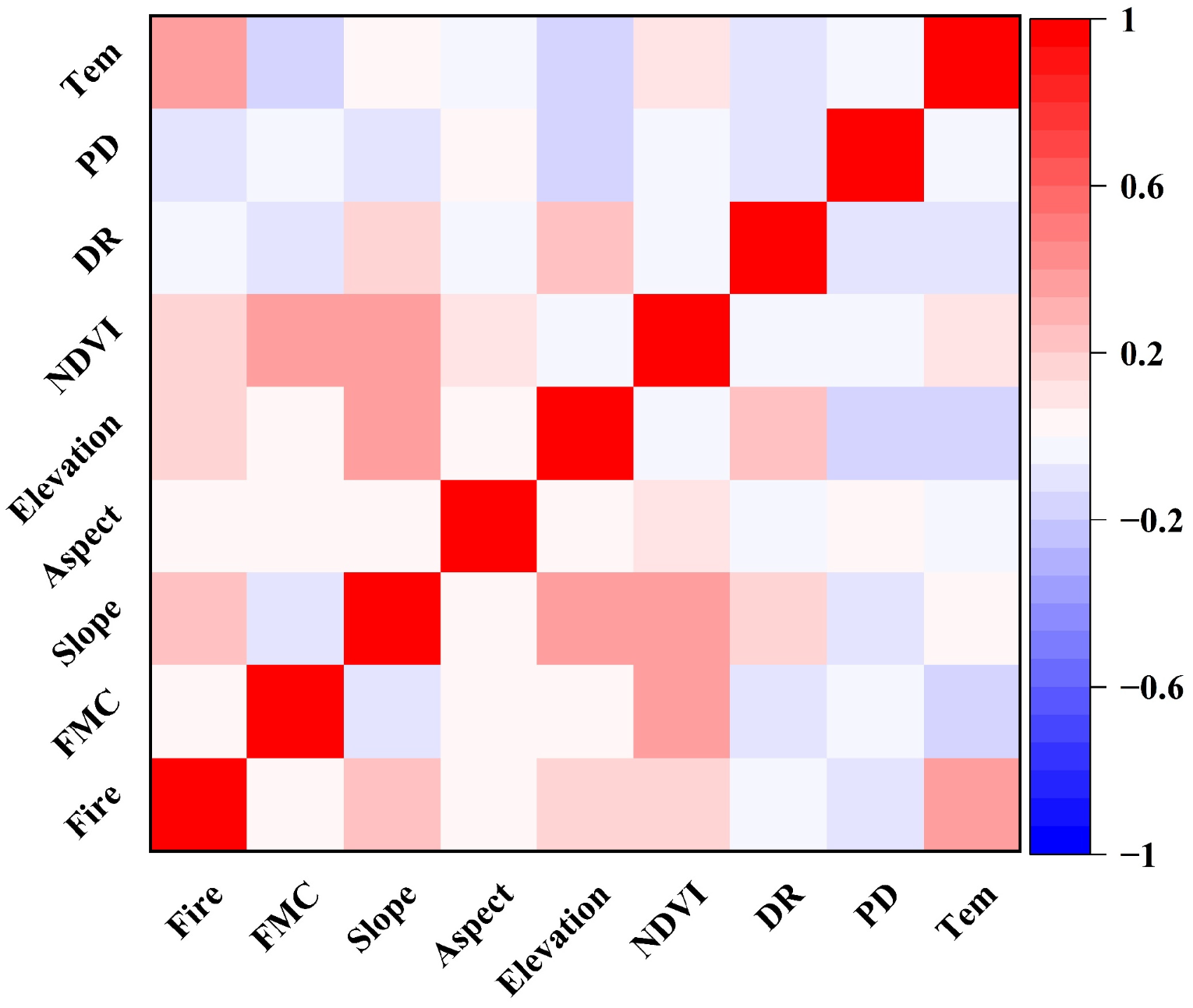
The Pearson correlation coefficient was utilized to quantitatively assess the linear association strength between driving factors and fire occurrence [49,50]. The results are presented in Table 3 and Figure 5. Temperature (r = 0.361) and slope (r = 0.241) displayed the most significant positive correlations with fire occurrence, suggesting that high-temperature conditions and steep terrain are crucial environmental factors contributing to fire occurrence. Elevation (r = 0.178) and NDVI (r = 0.185) also showed moderate positive correlations, indicating that high-altitude areas and regions with dense vegetation cover are also at an increased fire risk. FMC demonstrated a weak correlation with fire occurrence (r = 0.034), which can be ascribed to two factors: first, the temporal misalignment between fire point sampling and FMC observations; second, the potential presence of nonlinear threshold effects in FMC’s impact on fire risk, where FMC exerts significant heterogeneous effects on fire occurrence only when it falls below a certain critical value. Population density (r = −0.104) and distance to road (r = −0.031) showed negative correlations with fire occurrence, implying that although areas with intensive human activity and regions close to roads are potential ignition sources, their well-developed fire prevention facilities and rapid emergency response mechanisms can effectively reduce the probability of fire disasters. Analysis of inter-factor correlations revealed a moderate positive correlation between FMC and NDVI (r = 0.380), which is consistent with the eco-physiological characteristic that higher vegetation coverage corresponds to greater water-holding capacity. The positive correlations between slope and elevation (r = 0.373) and between slope and NDVI (r = 0.370) reflect the regulatory role of topography in vegetation spatial distribution. Temperature demonstrated a negative correlation with FMC (r = −0.156), which validates the physical mechanism that an increase in temperature accelerates vegetation transpiration and exacerbates fuel dryness. Overall, the absolute values of the correlation coefficients among all driving factors were below 0.4, and no highly collinear variable combinations were identified. This indicates that there are no severe multicollinearity issues among the selected factors, confirming their suitability for simultaneous inclusion in the subsequent machine learning modeling analysis.

4.1.2. Feature Importance and Interpretation of Key Factors

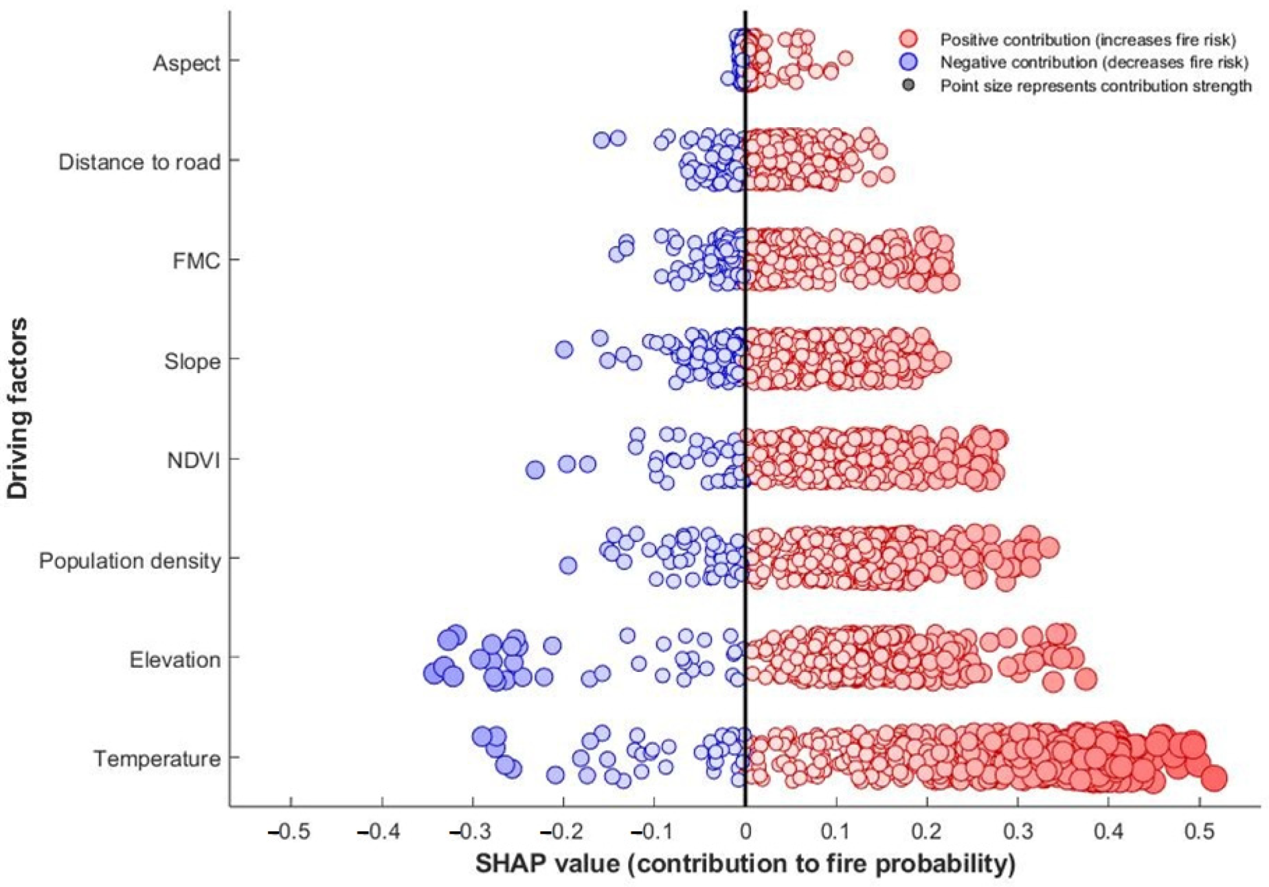
To elucidate the contribution mechanism of each driving factor to fire occurrence, this study performed SHAP analysis on 500 fire point samples from the test set, generating a feature contribution beeswarm plot (Figure 6). The results indicate that the contributions of these factors vary considerably. Temperature is identified as the most influential factor, featuring the broadest SHAP value distribution and being predominantly represented by red points. This implies that high temperature has a strong positive impact on the vast majority of fire point samples, serving as a crucial promoter of fire occurrence. Elevation ranks second, with its SHAP values presenting a distinct bidirectional distribution; positive contributions in some samples and negative contributions in others suggest a spatially heterogeneous influence on fire risk, which is associated with variations in vegetation type and human activity intensity at different altitudes. Population density ranks third, with predominantly red points indicating a significantly increased fire risk in areas with intensive human activity. NDVI ranks fourth, with SHAP values mainly represented by red points. This suggests that, within the study area, high vegetation coverage actually makes a positive contribution to fire occurrence, a phenomenon related to the vigorous vegetation growth during hot and dry seasons, which increases fuel loading. Slope ranks fifth, with relatively scattered SHAP values and coexisting positive and negative contributions. This pattern reflects the complex regulatory role of slope, which affects fire risk by regulating fuel distribution and fire spread rate. FMC ranks sixth, with its SHAP values also predominantly represented by red points. This indicates that FMC mainly makes positive contributions in the analyzed fire point samples, a pattern likely related to the concentration of samples in dry seasons or specific vegetation types. The distance to the road and the aspect are of relatively lower significance. The distance to the road exhibits weak positive contributions, which may be associated with the increased probability of ignition from human activities near roadways. The aspect demonstrates the most dispersed SHAP value distribution and the smallest magnitude of contribution, indicating that its influence on fire point samples is limited. Overall, temperature, elevation, and population density are the dominant factors driving the fire risk in the study area, whereas NDVI and FMC mainly contribute positively in the analyzed fire point samples.
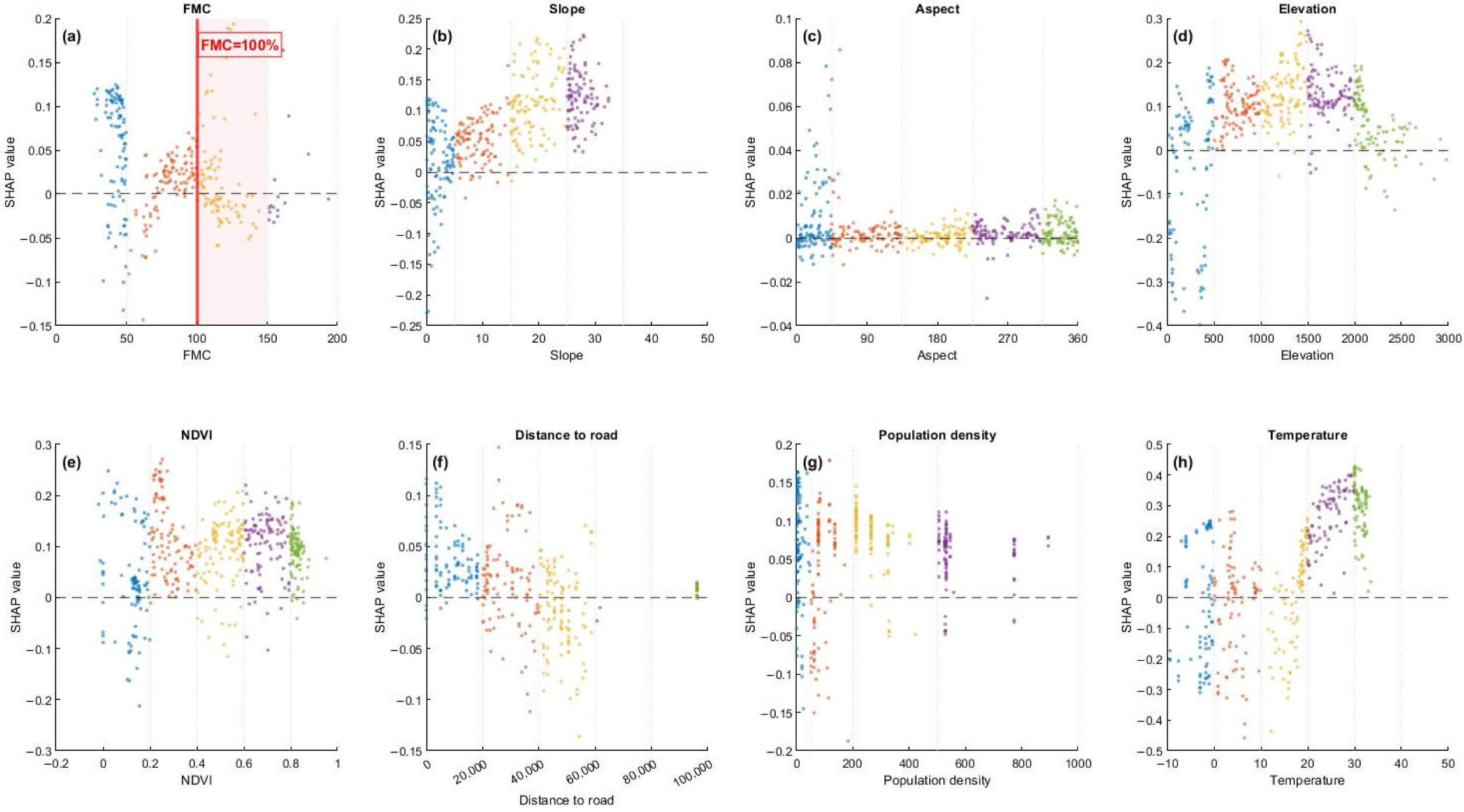
Based on the SHAP dependence plot (Figure 7), the influence of each driving factor on the probability of forest fire occurrence demonstrates significant nonlinear characteristics and threshold effects. The impact of the FMC on forest fires shows a negative correlation, featuring positive driving at low values and negative inhibition at high values. Specifically, within the 0%–50% interval, the SHAP values are predominantly positive, ranging from 0 to 0.1, which indicates that extreme dryness significantly elevates the risk of forest fires. In the 50%–100% interval, the positive values narrow to the range of 0–0.05, and the driving effect weakens. Negative values start to emerge in the 100%–150% interval. Excluding extreme values greater than 0.1, the concentration of positive values in this interval decreases. In the 150%–200% interval, the negative values increase significantly, with a distribution range from −0.1 to 0. A value of 100% can be regarded as a reference threshold for the shift in the risk direction. The slope exhibits a significant positive correlation, as the SHAP values continuously increase with the rise in the slope gradient. When the slope exceeds 10°, all values become positive and expand from the range of 0–0.1 to above 0–0.2, which reflects that steep terrain continuously enhances the risk of forest fires by facilitating fire spread, accelerating air circulation, and reducing the accessibility for fire suppression. The influence of the aspect is relatively weak, with the SHAP values mostly concentrated within the narrow range of −0.02 to +0.02, and both positive and negative values co-exist across different intervals. This indicates that its independent contribution is restricted and may be indirectly demonstrated through interactions with other factors. Elevation presents an inverted U-shaped nonlinear relationship. At elevations below 500 m, negative values are predominant, ranging from −0.4 to 0.2, which implies a lower risk at low altitudes. In the range of 500–1000 m, the values gradually change from negative to positive. The range of 1000–1500 m reaches a peak, with values concentrated between 0 and 0.3, signifying a high-risk elevation zone. In the range of 1500–2000 m, the values start to decrease. Above 2000 m, the negative values increase again, revealing that moderate elevations form a risk peak due to the combination of sufficient fuel load and favorable meteorological conditions. NDVI shows nonlinear positive driving characteristics. As NDVI increases, the positive SHAP values significantly outnumber the negative ones, indicating that areas with high vegetation cover offer abundant fuel conditions for fire occurrence. As a crucial indicator of vegetation biomass, the positive contribution of NDVI reflects the fundamental role of vegetation cover in fire risk formation—sufficiently high vegetation cover is a material prerequisite for fire occurrence. The distance to the road shows a trend of shifting from positive to negative. In the 0–20 km interval, positive values are dominant, ranging from 0 to 0.1, reflecting the dominant role of human activities near roads as a fire source. In the range of 20–40 km, the positive values weaken and negative values emerge. Within the 40–60 km interval, negative values are predominant, indicating that remote areas experience a reduced risk of forest fires due to the absence of ignition sources. Population density demonstrates a threshold effect, transitioning from positive to negative. In intervals of low population density, SHAP values are mostly positive, suggesting that areas with sparse populations face a higher risk of forest fires because of the lack of effective monitoring of fire sources and initial fire suppression measures. When the population density surpasses a certain threshold, SHAP values turn negative, reflecting that although densely populated areas have more ignition sources, well-established fire prevention facilities and rapid emergency response mechanisms effectively reduce the probability of fire occurrence. Temperature shows a significant positive correlation with a threshold effect. Below −10 °C, negative values are dominant, concentrated in the range of −0.3 to 0. Between −10 °C and 0 °C, negative values still prevail. Between 0 °C and 10 °C, both positive and negative values coexist, with negative values being more prevalent. Between 10 °C and 20 °C, positive values increase notably. When the temperature exceeds 20 °C, all values become positive, expanding from the range of 0–0.2 in the 20–30 °C interval to above 0–0.4 in the 30–40 °C interval. This indicates that high temperatures significantly enhance the risk of forest fires by accelerating the drying of fuel, reducing the moisture content of vegetation, and improving combustion conditions. A temperature of 20 °C can be regarded as a critical threshold for risk warning. The nonlinear characteristics and threshold effects of the eight aforementioned driving factors jointly disclose the multi-factor synergistic driving mechanism of forest fire risk. This offers a systematic scientific foundation for establishing a graded fire risk warning indicator system, pinpointing high-risk areas, and optimizing the allocation of fire prevention resources.

4.2. Modeling Results

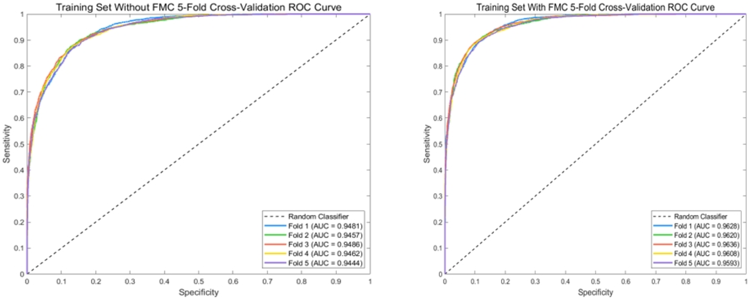
To evaluate the stability and generalization capacity of the models, a 5-fold cross-validation was carried out on the training set. Table 4 and Table 5, along with Figure 8, present a summary of the performance of the two models under 5-fold cross-validation. The baseline model without FMC attained an average AUC of 0.9451, an average accuracy of 86.8521%, an average precision of 82.3295%, an average recall of 87.7444%, and an average F1 score of 0.84938. In comparison, the model integrating dynamic FMC outperformed the baseline in all metrics. The average AUC increased to 0.9639, the average accuracy and precision rose to 89.0756% and 85.9564% respectively, and the average recall and F1 score improved to 89.3629% and 0.8737 respectively. The small standard deviations across folds imply that both models demonstrate good stability. Moreover, the confusion matrices disclose that after the incorporation of FMC, the number of false positives in each fold decreased substantially, while the number of true negatives increased correspondingly. This indicates that FMC mainly contributes to the reduction in the false positive rate. Simultaneously, the number of false negatives also decreased overall, suggesting that the model’s ability to identify fire points has been enhanced.
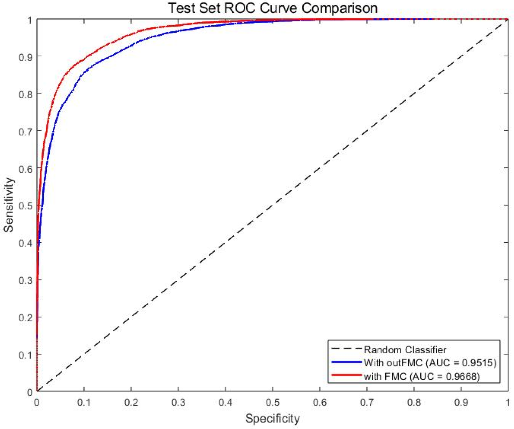
Table 6 and Figure 9 present the comparative experimental results between the baseline model without the FMC and the integrated model incorporating dynamic FMC. These results aim to further elucidate the specific contribution of dynamic FMC to model performance. The incorporation of the FMC variable led to comprehensive enhancements across all evaluation metrics. Specifically, from the confusion matrix, the number of true positives increased by 23, and the number of true negatives increased significantly by 293. Correspondingly, false positives and false negatives decreased by 293 and 23, respectively, indicating that the introduction of FMC significantly reduced the false-positive rate and also achieved some improvement in false negatives. In terms of specific metrics, accuracy increased from 87.40% to 89.61%, precision from 83.07% to 87.00%, recall from 88.08% to 89.18%, specificity from 86.36% to 89.94%, F1 score from 0.8584 to 0.8807, and AUC from 0.9515 to 0.9668. Among these, specificity and precision exhibited the most significant improvements, indicating that the dynamic FMC variable can effectively enhance the model’s ability to identify non-fire points, thereby substantially reducing false positives. Meanwhile, the improvement in AUC also implies a further enhancement in the model’s overall ability to distinguish between positive and negative samples.

4.3. Probability of Forest Fire Occurrence

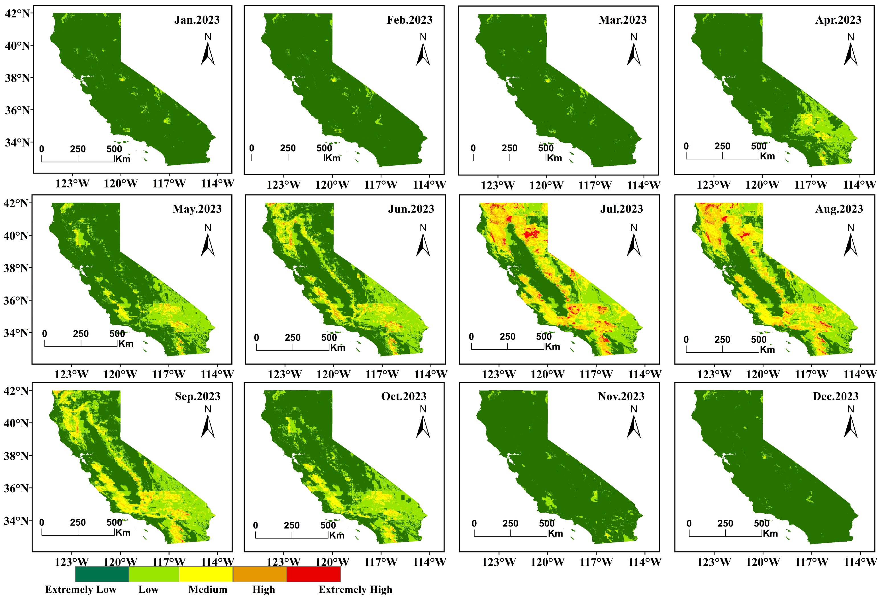
Figure 10 showcases a systematic analysis of the dynamic mapping outcomes for forest fire risk in California in 2023. Via continuous monthly forecasts and spatial heterogeneity analysis, the practical utility and application value of the model in regional-scale fire risk early warning are verified.
From a temporal perspective, the fire risk in California in 2023 demonstrated distinct seasonal progression patterns and nonlinear accumulation characteristics. From January to March (winter), the risk levels across the state remained low, with scarce and limited fire-related activities. This corresponded to the winter climate pattern, which was characterized by sufficient vegetation moisture and unfavorable conditions for burning. From April to May (spring), the risk gradually increased as temperatures rose and precipitation decreased. Concurrently, there was a significant increase in the frequency of fire occurrences, signifying the official start of the fire season. June was a critical month for the transition of the risk pattern. High-risk areas expanded rapidly, and the northern mountainous regions emerged as new risk-concentrated zones. During this period, the vegetation moisture across the state generally dropped below the critical thresholds, and dry wind systems became active, creating favorable conditions for fire outbreaks. July to August constituted the annual peak risk period, with August reaching the highest risk level of the year. During this phase, sustained high temperatures and drought reduced the vegetation moisture to the annual minimum levels. High-risk conditions persisted over extended periods, forming a widespread and long-lasting spatial threat pattern. The actual fire occurrences during this period accounted for a substantial proportion of the annual total. Notably, the risk accumulation process exhibited pronounced nonlinear acceleration characteristics. As the vegetation continued to dry, the rate of fire risk increase exceeded the linear change in dryness itself. This phenomenon validates the exponential enhancement effect of the vegetation drying process and reveals the amplification mechanism of water deficit on fire risk. In September, the risk started to decline gradually as temperatures decreased and humidity increased. Although it still remained at relatively high levels, this reflected the lag in the recovery of vegetation moisture. By October, with the advent of effective precipitation, high-risk areas contracted rapidly, and the statewide risk levels reverted to low values, signifying the end of the main fire season.
From a spatial perspective, the fire risk in California demonstrated significant regional heterogeneity. High-risk areas were mainly concentrated in the western slopes of the Sierra Nevada, the northern Coast Ranges, and the mountainous regions north of Los Angeles. These areas possess common features such as complex terrain, vegetation types mainly composed of flammable shrubs and coniferous forests, and frequent exposure to dry Santa Ana winds in summer. In contrast, the agricultural region of the Central Valley and the coastal urban areas consistently maintained low risk levels because of land-use types and local microclimatic influences. Notably, the spatial distribution of high-risk areas showed dynamic changes over the course of the seasons: the risk centers were primarily situated in the southern mountains in spring, expanded northward to encompass the entire Sierra Nevada in summer, and gradually shrank to localized hotspots in autumn. This dynamic evolution of spatial patterns is closely associated with vegetation phenology, topographic lifting effects, and seasonal variations in regional wind patterns.
Overall, the model effectively captured the entire dynamic process from risk accumulation and escalation to decline. The spatiotemporal evolution characteristics of the risk exhibited a high degree of consistency with the actual fire occurrence records. The complete risk lifecycle validates the efficacy of the Random Forest model incorporating dynamic FMC in characterizing the regional fire risk dynamics, offering a scientific foundation for the early warning of forest fires and the optimal allocation of fire-prevention resources in California and similar Mediterranean-type climate regions. This analysis further affirms that dynamic FMC, as a crucial link between meteorological conditions and vegetation response, is a key variable for enhancing the spatiotemporal prediction ability of fire risk models.
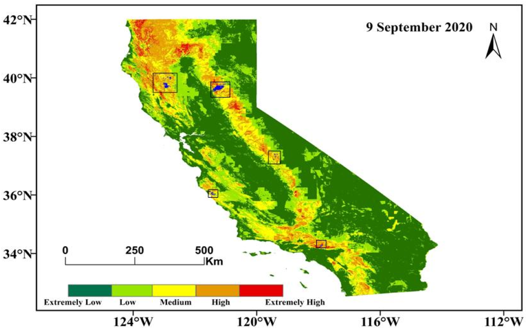
We selected 9 September 2020, a representative day marked by extremely high temperatures and drought, for a one-day fire risk analysis, as depicted in Figure 11. This specific date was chosen due to the occurrence of extremely high temperatures, arid conditions, and powerful winds in multiple regions of California, which represented one of the most significant periods of fire risk during that year. The spatial distribution map of fire risk generated by the model indicates that high-risk areas were predominantly concentrated on the western slopes of the Sierra Nevada, the northern Coast Ranges, and the mountainous regions north of Los Angeles, which is consistent with the spatial distribution of actual fire points on that day. At the sites of several major fire incidents, the model precisely identified high-risk levels, validating its capacity to characterize the spatial pattern of fire risk. This case study further substantiates the strong predictive capabilities of the Random Forest model incorporating dynamic FMC in complex fire risk environments.
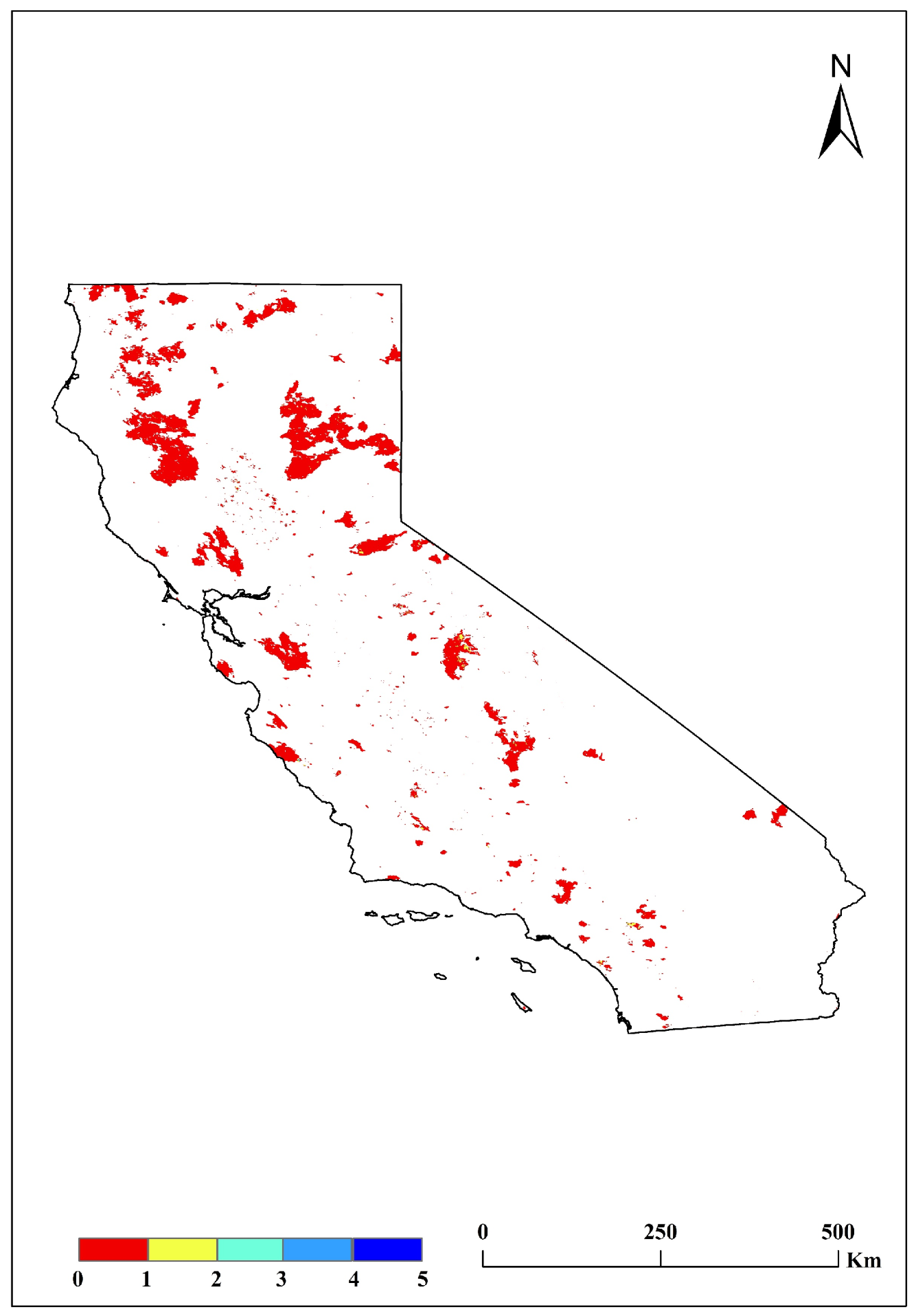
Figure 12 showcases a comparative analysis of the monthly prediction results for 2023 and the spatial distribution of fire points from 2020 to 2023, thereby further validating the stability and consistency of the model’s spatial prediction ability. The risk aggregation areas identified by the model display a high degree of spatial congruence with historical high-frequency fire occurrence regions, especially in the northern forest areas and the Sierra Nevada. This indicates that the model not only demonstrates a strong capacity for identifying current-year risks but also captures spatial risk patterns that comprehensively reflect the combined constraints of climate, vegetation, and topography in the region. The predicted risk levels exhibit a significant positive correlation with the four-year spatial frequency of fire points at the pixel scale. This suggests that the model can not only differentiate between high-risk and low-risk areas at the regional scale but also discern subtle differences in risk levels within the same area at a finer spatial resolution, and these differences are consistent with the long-term statistical patterns of fire occurrence.

5. Discussion

This study utilizes a newly developed high-spatiotemporal-resolution dynamic FMC monitoring product to establish a novel fire risk prediction framework that integrates dynamic FMC states. Through an analysis of historical fire cases, the physical basis of FMC as a key causative factor is first established. Subsequently, the advantages and implications of integrating dynamic FMC into machine learning models for enhancing prediction accuracy and characterizing risk evolution are systematically expounded.

5.1. Physical Linkage Between FMC and Fire Occurrence: Empirical Evidence from Typical Fire Cases

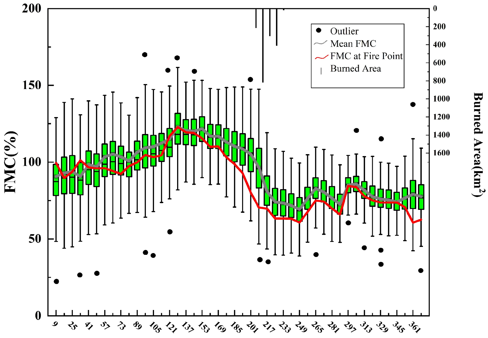
To clarify the inherent relationship between the Fine FMC and the occurrence and development of forest fires, this study selected the 2021 Dixie Fire in California as a representative case for analysis. As shown in Figure 13, the temporal evolution of FMC in the fire-affected area demonstrated distinct phase characteristics. During the pre-fire phase (from May to June), FMC underwent a significant decline approximately 4 to 6 weeks before the fire ignition, suggesting that the vegetation had entered a rapid drying process before the summer peak. Once FMC dropped below a critical threshold, the vegetation shifted from a fire-barrier medium to a fire-propagating medium, leading to a non-linear increase in fire risk. During the fire occurrence and spread phase (from July to August), FMC remained consistently low, providing stable dry conditions for fire propagation and potentially establishing a positive feedback loop: “Low FMC promotes fire, and fire maintains dry conditions.” In the post-fire recovery phase (after September), FMC gradually recovered with the arrival of precipitation; however, its recovery was significantly delayed compared to the change in meteorological conditions, showing a pronounced moisture lag effect. This complete temporal sequence, “Pre-fire drought accumulation, sustained low levels during the fire, and lagged post-fire recovery,” confirms that FMC serves as a key threshold indicator for fire risk, a pre-warning indicator, and a crucial link between meteorological conditions and fuel states. Relying solely on static environmental factors or average meteorological data cannot capture these temporal fluctuations closely associated with real-time vegetation moisture stress. This limitation is the core motivation and physical basis for integrating dynamic FMC into the machine learning model in this study, thus improving model performance and providing mechanistic explanations.

5.2. Enhancement Effect of Dynamic FMC on Model Performance and Mechanistic Interpretation

Based on the aforementioned physical relationships, this study further quantified the marginal contribution of dynamic FMC to wildfire risk prediction models via comparative experiments. The results indicate that the incorporation of FMC results in systematic improvements across all evaluation metrics of the random forest model. This finding has significant practical implications, suggesting an enhanced sensitivity in detecting actual wildfire events. Specifically, the model becomes more efficient in identifying potential fire occurrences that are frequently overlooked by traditional approaches, thus reducing the risk of missed detections. Meanwhile, the concurrent improvement of multiple evaluation metrics validates that the incorporation of FMC does not undermine classification accuracy; rather, it realizes a significant enhancement of the model’s overall performance.
From a mechanistic perspective, the contribution of the FMC stems from its capacity to dynamically characterize the evolution of wildfire risk. Conventional static models, which are predominantly based on topographic features and long-term climatic averages, can only capture the “background probability” of fire occurrence and are inadequate to reflect rapid drought processes at weather timescales. In contrast, the FMC functions as a crucial bridge that links meteorological conditions and vegetation responses, effectively capturing the cumulative effects of vegetation water stress and its potential threshold transitions. As demonstrated in the Dixie Fire case, a significant decline in the FMC often precedes wildfire outbreaks by several weeks. This early signal endows the model with temporal predictive capability, enabling it not only to identify areas with high risk but also to more precisely determine when the risk is likely to increase. Moreover, the low collinearity among predictors (with correlation coefficients below 0.4) ensures that the FMC is incorporated as an independent source of information, rather than as redundant input, thereby enabling the model to fully leverage its predictive value.

5.3. Synergistic Effects and Regional Specificity of Wildfire Drivers

Building upon the validation of the model’s performance, this study conducted a further analysis of the contribution of key driving factors to wildfire occurrence. In line with previous studies, temperature (r = 0.361) has been identified as the dominant driver, ranking first in both correlation analysis and feature importance. This validates the fundamental role of high temperature in promoting wildfire occurrence. Beyond this general trend, the temperature in California’s Mediterranean climate demonstrates a cascading amplification effect. In addition to directly providing favorable thermal conditions for combustion, temperature indirectly exacerbates vegetation water stress through its negative correlation with FMC (r = −0.156). This coupled heat–dryness mechanism elucidates why the wildfire risk continues to increase during the August peak period even when the temperature rise decelerates, highlighting the significance of incorporating dynamic FMC.
Topographic factors, such as slope (r = 0.241) and elevation (r = 0.178), exhibit positive correlations with the occurrence of wildfires, which reflects their role in promoting fire spread and restricting suppression efficiency. Their interactions with the NDVI (r = 0.370) and elevation (r = 0.373) further demonstrate that topography indirectly influences fire risk by affecting vegetation and the local micro-climate. In contrast, population density shows a weak negative correlation (r = −0.104). This likely reflects the efficacy of fire management and rapid response systems in densely populated areas of California. It implies that human activities not only serve as ignition sources but also contribute to mitigating wildfire risk.

5.4. Limitations and Future Directions

Despite the promising predictive performance attained in this study, several limitations ought to be recognized. Firstly, at the data level, wildfire occurrence records predominantly depend on satellite observations and ground reports, which might overlook early-stage or small-scale fires, thereby introducing potential bias in the training samples. Moreover, the spatial resolution of remotely sensed FMC products remains relatively coarse, restricting their capacity to capture fine-scale heterogeneity in vegetation moisture. Secondly, while the model effectively predicts the probability of wildfire occurrence, it fails to account for post-ignition fire behavior, such as spread rate, fire intensity, or spotting distance, which restricts its applicability in real-time fire management. Thirdly, although temperature is identified as the dominant driver, the generalizability of the model under future climate conditions remains uncertain, especially as the frequency and intensity of extreme events (e.g., dry thunderstorms and Santa Ana winds) may exceed the range represented in historical training data.
Future research can be advanced in several directions. Firstly, the integration of multi-source remote sensing data, such as Sentinel-1 SAR for vegetation moisture and GEDI LiDAR for vegetation structure, may enhance the spatiotemporal representation of FMC and fuel characteristics. Secondly, the coupling with physical fire behavior models would allow for a shift from predicting ignition probability to simulating the entire wildfire process, encompassing ignition, spread, and impacts. Thirdly, the incorporation of climate model projections could support wildfire risk assessment under future climate scenarios, offering a scientific foundation for long-term fire management and adaptation strategies.

6. Conclusions

This study tackles the inadequate consideration of a crucial internal factor, FMC, in existing wildfire prediction models. Concentrating on California, USA, a wildfire occurrence probability model based on the random forest algorithm was developed by integrating a dynamically retrieved FMC product with multi-source geospatial data. Through comparative experiments and interpretability analysis, the contribution of dynamic FMC and the dominant drivers of regional wildfire risk were systematically examined. The main conclusions are as follows:
(1)
Dynamic FMC significantly improves model performance. Compared with the baseline model without FMC, the incorporation of FMC increases accuracy, precision, recall, specificity, and F1 score by 2.21%, 3.93%, 0.37%, 3.60%, and 0.0223, respectively, indicating that dynamic FMC can effectively enhance the model’s ability to identify non-fire points. This is crucial for minimizing false positives.
(2)
FMC functions as a leading indicator of wildfire risk. Case analyses demonstrate that a sharp decrease in FMC precedes wildfire outbreaks by approximately 4–6 weeks. Its temporal pattern—pre-fire drought accumulation, consistently low levels during fire events, and delayed post-fire recovery—emphasizes its role as a key connection between meteorological conditions and fuel status. This dynamic behavior enables the model to capture not only the locations with high risk but also the times when the risk is likely to increase, reflecting the nonlinear amplification of the heat–dryness coupling mechanism.
(3)
The synergistic effects of factors contributing to wildfires are elucidated. Temperature is recognized as the predominant factor, directly promoting combustion and indirectly exacerbating vegetation water stress due to its inverse relationship with the FMC. Topographic factors, namely slope and elevation, determine the spatial distribution of high-risk areas by affecting vegetation and the microclimate. Population density reflects the dual influence of human activities, serving both as an ignition source and a regulator of fire risk. The low collinearity among variables (correlation coefficients < 0.4) guarantees that FMC can be effectively employed as an independent information source.
(4)
The model exhibits a robust capacity for regional-scale dynamic risk mapping. The monthly wildfire risk maps for California in 2023 effectively capture the complete seasonal cycle of wildfire risk, from the spring build-up to the summer peak and the autumn decline. The spatial distribution of high-risk areas is highly consistent with historical fire occurrence patterns, indicating the model’s potential for accurate early warning and optimized fire management in regions with a Mediterranean climate.

Author Contributions

Conceptualization, Y.L. (Yuanzong Li) and C.Z.; methodology, Y.L. (Yuanzong Li), C.Z., and J.Z.; validation, Y.L. (Yuanzong Li), C.Z., J.Z., W.W., Z.C., and Y.L. (Yongfeng Luo); formal analysis, Y.L. (Yuanzong Li), C.Z., and J.Z.; investigation, Y.L. (Yuanzong Li), C.Z., J.Z., and W.W.; resources, Y.L. (Yuanzong Li); data curation, J.Z.; writing—original draft preparation, Y.L. (Yuanzong Li); writing—review and editing, Y.L. (Yuanzong Li) and C.Z.; supervision, C.Z.; project administration, C.Z., J.Z., W.W., and Y.L. (Yuanzong Li); funding acquisition, C.Z. All authors have read and agreed to the published version of the manuscript.

Funding

This research was funded by the National Natural Science Foundation of China (Nos. 42474052 and 42030112) and the Hunan Science Fund for Distinguished Young Scholars (2024JJ2100).

Data Availability Statement

The remote sensing data supporting this study are publicly available and can be accessed and processed using Google Earth Engine (GEE) platform. The California fuel moisture content dataset supporting the findings of this study are available on request from Yuanzong Li (20231100004@csuft.edu.cn). The data are not publicly available due to privacy.

Acknowledgments

Many thanks to NASA and USGS for generously providing the datasets free of charge.

Conflicts of Interest

The authors declare no conflicts of interest. The authors declare that they have no known competing financial interests or personal relationships that could have potentially influenced the work reported in this paper.

References

  1. Agee, J.K.; Finney, M.; Gouvenain, R.D. Forest fire history of desolation peak, Washington. Can. J. For. Res. 1990, 20, 350–356. [Google Scholar] [CrossRef] [Scilit]
  2. Littell, J.S.; Peterson, D.L.; Riley, K.L.; Liu, Y.; Luce, C.H. A review of the relationships between drought and forest fire in the United States. Glob. Change Biol. 2016, 22, 2353–2369. [Google Scholar] [CrossRef] [Scilit]
  3. Bonazountas, M.; Kallidromitou, D.; Kassomenos, P.A.; Passas, N. Forest fire risk analysis. Hum. Ecol. Risk Assess. 2005, 11, 617–626. [Google Scholar] [CrossRef] [Scilit]
  4. Zhang, P.; Yan, P.; Liu, H. A Quantitative Analysis of Chinese and International Studies on Forest Fire Prediction from 2002 to 2019. J. Wildland Fire Sci. 2023, 41, 53–59. [Google Scholar]
  5. Pham, B.T.; Jaafari, A.; Avand, M.; Al-Ansari, N.; Dinh Du, T.; Yen, H.P.H.; Phong, T.V.; Nguyen, D.H.; Le, H.V.; Mafi-Gholami, D.; et al. Performance evaluation of machine learning methods for forest fire modeling and prediction. Symmetry 2020, 12, 1022. [Google Scholar] [CrossRef] [Scilit]
  6. Preisler, H.K.; Ager, A.A. Forest-Fire ModelsBased in part on the article “Forest fire models” by Haiganoush K. Preisler and David R. Weise, which appeared in the Encyclopedia of Environmetrics. Encycl. Environmetrics 2013. [Google Scholar] [CrossRef] [Scilit]
  7. Ning, J.; Liu, H.; Yu, W.; Deng, J.; Sun, L.; Yang, G.; Wang, M.; Yu, H. Comparison of different models to simulate forest fire spread: A case study. Forests 2024, 15, 563. [Google Scholar] [CrossRef] [Scilit]
  8. Zheng, S.; Gao, P.; Wang, W.; Zou, X. A highly accurate forest fire prediction model based on an improved dynamic convolutional neural network. Appl. Sci. 2022, 12, 6721. [Google Scholar] [CrossRef] [Scilit]
  9. Singh, K.R.; Neethu, K.; Madhurekaa, K.; Harita, A.; Mohan, P. Parallel SVM model for forest fire prediction. Soft Comput. Lett. 2021, 3, 100014. [Google Scholar] [CrossRef] [Scilit]
  10. Sun, X.; Li, N.; Chen, D.; Chen, G.; Sun, C.; Shi, M.; Gao, X.; Wang, K.; Hezam, I.M. A forest fire prediction model based on cellular automata and machine learning. IEEE Access 2024, 12, 55389–55403. [Google Scholar] [CrossRef] [Scilit]
  11. Fangrong, Z.; Yuning, G.; Guochao, Q.; Yi, M.; Guofang, W. Multi-factor coupled forest fire model based on cellular automata. J. Saf. Sci. Resil. 2024, 5, 413–421. [Google Scholar] [CrossRef] [Scilit]
  12. Feng, Z.; Zhao, Z.; Chen, S.; Zhang, H. Research on Multi-Factor Forest Fire Prediction Model Using Machine Learning Method in China. ResearchSquare 2020. [Google Scholar] [CrossRef]
  13. Jingjing, P.; Haoying, Z.; Shiyu, Y.; Mengyao, W.; Yun, L. Research on forest fire risk assessment and prevention and control Countermeasures: A case study of Qinyuan County, Shanxi Province, China. Ecol. Indic. 2025, 176, 113719. [Google Scholar] [CrossRef] [Scilit]
  14. Chang, L.; Zhi, Y.; Binbin, Z.; Sihang, Z. Wildfire risk assessment using multi-source remote sensing data and GIS. In 2024 IEEE 4th International Conference on Information Technology, Big Data and Artificial Intelligence (ICIBA); IEEE: New York, NY, USA, 2024. [Google Scholar]
  15. Bisquert, M.; Caselles, E.; Sánchez, J.M.; Caselles, V. Application of artificial neural networks and logistic regression to the prediction of forest fire danger in Galicia using MODIS data. Int. J. Wildland Fire 2012, 21, 1025–1029. [Google Scholar] [CrossRef] [Scilit]
  16. Jafari Goldarag, Y.; Mohammadzadeh, A.; Ardakani, A. Fire risk assessment using neural network and logistic regression. J. Indian Soc. Remote Sens. 2016, 44, 885–894. [Google Scholar] [CrossRef] [Scilit]
  17. Guo, F.; Zhang, L.; Jin, S.; Tigabu, M.; Su, Z.; Wang, W. Modeling anthropogenic fire occurrence in the boreal forest of China using logistic regression and random forests. Forests 2016, 7, 250. [Google Scholar] [CrossRef] [Scilit]
  18. Guo, F.; Wang, G.; Su, Z.; Liang, H.; Wang, W.; Lin, F.; Liu, A. What drives forest fire in Fujian, China? Evidence from logistic regression and Random Forests. Int. J. Wildland Fire 2016, 25, 505–519. [Google Scholar] [CrossRef] [Scilit]
  19. Milanović, S.; Marković, N.; Pamučar, D.; Gigović, L.; Kostić, P.; Milanović, S.D. Forest fire probability mapping in eastern Serbia: Logistic regression versus random forest method. Forests 2020, 12, 5. [Google Scholar] [CrossRef] [Scilit]
  20. Bian, R.; Chen, K.; Li, G.; Wang, Z.; Qiu, Y.; Bai, H.; Kong, W. Evaluation of three algorithms and forest fire risk prediction in zhejiang province of china. Forests 2024, 15, 2146. [Google Scholar] [CrossRef] [Scilit]
  21. Gao, C.; Lin, H.; Hu, H. Forest-fire-risk prediction based on random forest and backpropagation neural network of Heihe area in Heilongjiang province, China. Forests 2023, 14, 170. [Google Scholar] [CrossRef] [Scilit]
  22. Li, S.; Zhang, F.; Lin, H. Research on forest fire risk evaluation based on machine learning algorithm. J. Nanjing For. Univ. 2023, 47, 49–56. [Google Scholar]
  23. Lee, J.; Ahn, S.; Im, S. Spatial Prediction of Forest Fire Occurrence Integrating Human Proximity: A Machine Learning Approach for Korea’s Eastern Coast. Forests 2026, 17, 281. [Google Scholar] [CrossRef] [Scilit]
  24. He, H.S.; Shang, B.Z.; Crow, T.R.; Gustafson, E.J.; Shifley, S.R. Simulating forest fuel and fire risk dynamics across landscapes—LANDIS fuel module design. Ecol. Model. 2004, 180, 135–151. [Google Scholar] [CrossRef] [Scilit]
  25. Ager, A.A.; Vaillant, N.M.; Finney, M.A. Integrating fire behavior models and geospatial analysis for wildland fire risk assessment and fuel management planning. J. Combust. 2011, 2011, 572452. [Google Scholar] [CrossRef] [Scilit]
  26. Perello, N.; Trucchia, A.; D’andrea, M.; Meschi, G.; Ghasemiazma, F.; Degli Esposti, S.; Fiorucci, P.; Ferraris, L.; Gollini, A.; Negro, D. Fuel-aware forest fire danger rating system RISICO: A comparative study for Italy. Int. J. Wildland Fire 2025, 34, WF25023. [Google Scholar] [CrossRef] [Scilit]
  27. Danson, F.M.; Bowyer, P. Estimating live fuel moisture content from remotely sensed reflectance. Remote Sens. Environ. 2004, 92, 309–321. [Google Scholar] [CrossRef] [Scilit]
  28. Yebra, M.; Chuvieco, E.; Riano, D. Estimation of live fuel moisture content from MODIS images for fire risk assessment. Agric. For. Meteorol. 2008, 148, 523–536. [Google Scholar] [CrossRef] [Scilit]
  29. García, M.; Chuvieco, E.; Nieto, H.; Aguado, I. Combining AVHRR and meteorological data for estimating live fuel moisture content. Remote Sens. Environ. 2008, 112, 3618–3627. [Google Scholar] [CrossRef] [Scilit]
  30. Che, X.; Feng, M.; Sexton, J.O.; Channan, S.; Yang, Y.; Sun, Q. Assessment of MODIS BRDF/Albedo model parameters (MCD43A1 Collection 6) for directional reflectance retrieval. Remote Sens. 2017, 9, 1123. [Google Scholar] [CrossRef] [Scilit]
  31. Modis, T.A. MCD43 v006/v006, 1 User Guide Introduction; NASA Land Processes Distributed Active Archive Center: Sioux Falls, SD, USA, 2021. [Google Scholar] [CrossRef]
  32. Van Zyl, J.J. The Shuttle Radar Topography Mission (SRTM): A breakthrough in remote sensing of topography. Acta Astronaut. 2001, 48, 559–565. [Google Scholar] [CrossRef] [Scilit]
  33. Hersbach, H.; Bell, B.; Berrisford, P.; Hirahara, S.; Horányi, A.; Muñoz-Sabater, J.; Nicolas, J.; Peubey, C.; Radu, R.; Schepers, D.; et al. The ERA5 global reanalysis. Q. J. R. Meteorol. Soc. 2020, 146, 1999–2049. [Google Scholar] [CrossRef] [Scilit]
  34. Dobson, J.E.; Bright, E.A.; Coleman, P.R.; Durfee, R.C.; Worley, B.A. LandScan: A global population database for estimating populations at risk. Photogramm. Eng. Remote Sens. 2000, 66, 849–857. [Google Scholar]
  35. Lebakula, V.; Sims, K.; Reith, A.; Rose, A.; McKee, J.; Coleman, P.; Kaufman, J.; Urban, M.; Jochem, C.; Whitlock, C.; et al. LandScan global 30 arcsecond annual global gridded population datasets from 2000 to 2022. Sci. Data 2025, 12, 495. [Google Scholar] [CrossRef] [Scilit]
  36. Giglio, L.; Boschetti, L.; Roy, D.P.; Humber, M.L.; Justice, C.O. The Collection 6 MODIS burned area mapping algorithm and product. Remote Sens. Environ. 2018, 217, 72–85. [Google Scholar] [CrossRef] [Scilit] [PubMed]
  37. Shantal, M.; Othman, Z.; Bakar, A.A. A novel approach for data feature weighting using correlation coefficients and min–max normalization. Symmetry 2023, 15, 2185. [Google Scholar] [CrossRef] [Scilit]
  38. Rigatti, S.J. Random forest. J. Insur. Med. 2017, 47, 31–39. [Google Scholar] [CrossRef] [Scilit]
  39. Salman, H.A.; Kalakech, A.; Steiti, A. Random forest algorithm overview. Babylon. J. Mach. Learn. 2024, 2024, 69–79. [Google Scholar] [CrossRef] [Scilit] [PubMed]
  40. Parmar, A.; Katariya, R.; Patel, V. A review on random forest: An ensemble classifier. In International Conference on Intelligent Data Communication Technologies and Internet of Things; Springer: Berlin/Heidelberg, Germany, 2018. [Google Scholar]
  41. Zien, A.; Krämer, N.; Sonnenburg, S.; Rätsch, G. The feature importance ranking measure. In Joint European Conference on Machine Learning and Knowledge Discovery in Databases; Springer: Berlin/Heidelberg, Germany, 2009. [Google Scholar]
  42. Hooker, S.; Erhan, D.; Kindermans, P.J.; Kim, B. Evaluating feature importance estimates. arXiv 2018, arXiv:1806.10758. [Google Scholar]
  43. Wojtas, M.; Chen, K. Feature importance ranking for deep learning. Adv. Neural Inf. Process. Syst. 2020, 33, 5105–5114. [Google Scholar]
  44. Van den Broeck, G.; Lykov, A.; Schleich, M.; Suciu, D. On the tractability of SHAP explanations. J. Artif. Intell. Res. 2022, 74, 851–886. [Google Scholar] [CrossRef] [Scilit]
  45. Li, Z. Extracting spatial effects from machine learning model using local interpretation method: An example of SHAP and XGBoost. Comput. Environ. Urban Syst. 2022, 96, 101845. [Google Scholar] [CrossRef] [Scilit]
  46. Wang, H.; Liang, Q.; Hancock, J.T.; Khoshgoftaar, T.M. Feature selection strategies: A comparative analysis of SHAP-value and importance-based methods. J. Big Data 2024, 11, 44. [Google Scholar] [CrossRef] [Scilit]
  47. Naidu, G.; Zuva, T.; Sibanda, E.M. A review of evaluation metrics in machine learning algorithms. In Computer Science On-Line Conference; Springer: Berlin/Heidelberg, Germany, 2023. [Google Scholar]
  48. Vujović, Ž. Classification model evaluation metrics. Int. J. Adv. Comput. Sci. Appl. 2021, 12, 599–606. [Google Scholar] [CrossRef] [Scilit]
  49. Gogtay, N.J.; Thatte, U.M. Principles of correlation analysis. J. Assoc. Physicians India 2017, 65, 78–81. [Google Scholar]
  50. Franzese, M.; Iuliano, A. Correlation analysis. In Encyclopedia of Bioinformatics and Computational Biology: ABC of Bioinformatics; Elsevier: Amsterdam, The Netherlands, 2018; pp. 706–721. [Google Scholar]
Figure 1. (a) Geographical location of the study area. (b) Elevation of the study area.
Forests 17 00532 g001
Figure 2. Monthly FMC data for California in 2023.
Forests 17 00532 g002
Figure 3. Comparison of Observed and Model-Predicted FMC Across Vegetation Types Using Multi-Source Data Fusion.
Forests 17 00532 g003
Figure 4. Spatial distribution of driving factors.
Forests 17 00532 g004
Figure 5. Heatmap of Pearson Correlation Matrix for Forest Fire Driving Factors.
Forests 17 00532 g005
Figure 6. SHAP Summary Plot of the Random Forest-Based Fire Occurrence Model.
Forests 17 00532 g006
Figure 7. SHAP dependence plots of eight predictors in the Random Forest fire occurrence model. (a) FMC SHAP value; (b) Slop SHAP value; (c) Aspect SHAP value; (d) Elevation SHAP value; (e) NDVI SHAP value; (f) Distance to road SHAP value; (g) Population density SHAP value; (h) Temperature SHAP value.
Forests 17 00532 g007
Figure 8. Comparison of 5-fold cross-validation ROC curves on the training set.
Forests 17 00532 g008
Figure 9. ROC curve comparison of the two models on the test set.
Forests 17 00532 g009
Figure 10. Spatial distribution of monthly fire risk levels in California, 2023.
Forests 17 00532 g010
Figure 11. Fire risk distribution overlaid with 9 September 2020 burned areas. The blue area inside the box indicates the burned area of that day.
Forests 17 00532 g011
Figure 12. Spatial frequency distribution of fire points in California from 2020 to 2023.
Forests 17 00532 g012
Figure 13. Temporal dynamics of FMC and burned area during the 2021 fire season.
Forests 17 00532 g013
Table 1. Vegetation-Adapted FMC Model Performance Indicators.
Vegetation TypeR2RMSE (%)Bias
Coniferous forest0.635312.728−1.7946
Broadleaf forest0.687416.8867−0.4009
Open shrubland0.546721.73740.4594
Closed shrubland0.619414.8287−1.3701
Grassland0.751114.31173.2288
Sparse vegetation0.607514.8237−2.6594
Table 2. Forest Fire Driving Factors Considered in the Model.
Variable NameFactor NameData Source
TopographySlopeUSGS, Reston, USA
Aspect
Elevation
MeteorologyTemperatureECMWF (for ERA5), Reading, United Kingdom
VegetationNDVINASA (for MODIS), Washington, D.C., USA
FMC
Human ActivityPopulation DensityOak Ridge National Laboratory (for LandScan), Oak Ridge, USA
Distance to RoadEsri (for World Roads), Redlands, USA
Table 3. Correlation Analysis of Fire Driving Factors.
VariableFMCSlopeAspectElevationNDVIDistance to RoadPopulation DensityTemperature
FMC1
Slope−0.1111
Aspect0.0090.0581
Elevation0.0120.3730.0321
NDVI0.3800.3700.090−0.0121
Distance to Road−0.1200.170−0.0180.203−0.0351
Population Density−0.056−0.1110.015−0.156−0.051−0.1271
Temperature−0.1560.029−0.013−0.1690.068−0.091−0.0181
Table 4. Confusion matrices for both models (5-fold cross-validation).
ModelFoldTPTNFPFN
Without FMC125693284494325
224693318516351
324313336509388
423713376535381
525313262602281
With
FMC
125453451327349
225323420414288
324623443402357
424483446465304
525373424440275
Table 5. The 5-fold cross-validation performance of the two models on the training dataset.
ModelFoldAUCAccuracy (%)Precision (%)Recall (%)Specificity (%)F1 Score
Without FMC10.949987.724883.872088.769986.92430.8625
20.947986.970282.713687.553286.54150.8506
30.940086.539682.687186.236386.76200.8442
40.940786.252481.589886.155586.32060.8381
50.946986.773580.785290.007184.42030.8515
With
FMC
10.965689.868188.614287.940691.34460.8828
20.963189.150085.947089.787489.20190.8783
30.960488.610485.963787.335989.54490.8664
40.967588.459784.037188.953588.11050.8643
50.962889.290085.220090.220588.61280.8765
Table 6. Test set performance comparison of the two models.
MetricWithout FMCWith FMCImprovement
TP5456547923
TN70337326293
FP1112819−293
FN688665−23
AUC0.95150.96680.0153
Accuracy (%)87.4089.612.21
Precision (%)83.0787.003.93
Recall (%)88.0889.180.37
Specificity (%)86.3589.943.60
F1 Score0.85840.88070.0223
Disclaimer/Publisher’s Note: The statements, opinions and data contained in all publications are solely those of the individual author(s) and contributor(s) and not of MDPI and/or the editor(s). MDPI and/or the editor(s) disclaim responsibility for any injury to people or property resulting from any ideas, methods, instructions or products referred to in the content.