Article

Microtopographic and Hydrological Response to Repeated Seismic Line Disturbance in a Boreal Fen of Northern Alberta, Canada
1
Department of Geography, University of Calgary, Calgary, AB T2N 1N4, Canada
2
Canadian Forest Service, Natural Resources Canada, Ottawa, ON P6A 2E5, Canada
*
Author to whom correspondence should be addressed.
Forests 2026, 17(4), 489; https://doi.org/10.3390/f17040489
Submission received: 2 March 2026 / Revised: 7 April 2026 / Accepted: 13 April 2026 / Published: 15 April 2026
(This article belongs to the Special Issue The Impact of Disturbances on Forest Restoration and Regeneration)

Abstract

Seismic lines are among the most widespread anthropogenic disturbances in Alberta’s boreal peatlands, where repeated petroleum-exploration surveys can alter surface morphology, hydrology, and recovery potential. Although low-impact seismic (LIS) techniques are designed to minimize ground disturbance, the long-term consequences of re-using existing lines remain poorly understood. This study used remotely piloted aircraft system (RPAS)-based LiDAR and optical imagery to examine how peatland microtopography and hydrology evolve following repeated seismic surveys. We quantified four attributes—ground depression, hummock cover, depth to water, and surface water cover—across new seismic lines (cut in 2021), old seismic lines (cut in 1996), and re-disturbance (cut in 1996, re-cut in 2021) LIS lines, as well as adjacent undisturbed peatland, in a boreal fen of northern Alberta. New disturbances were depressed by approximately 10 cm relative to the surrounding peatland and exhibited reduced microtopographic variability. Hummock cover decreased from 21% in the matrix to 6% on new disturbances. Old disturbances showed greater heterogeneity than new disturbances, with hummock cover partially recovering to 14% and surface water increasing from 7% to 27%, reflecting greater spatial heterogeneity in surface conditions. Re-disturbances exhibited microtopographic conditions similar to or more degraded than old disturbances, with hummock cover reduced to 2% and persistently high surface water cover (27%). These patterns suggest that repeated seismic surveys may limit recovery and maintain altered hydrological and microtopographic conditions. Within the context of this case study, even narrow LIS corridors were associated with persistent alterations when re-used, highlighting the importance of considering re-use effects when developing management strategies for peatland ecosystems. RPAS data provide an effective means to quantify these fine-scale changes and inform peatland restoration and seismic line management.

1. Introduction

Boreal peatlands are a defining feature of Alberta’s northern landscapes. These wetlands are characterized by accumulation of partially decayed organic matter (peat) [1]. In Canada, organic deposits thicker than 40 cm are classified as peatlands [2]. Peatlands cover about 16% of Alberta and serve as major carbon stores and key habitat for woodland caribou (Rangifer tarandus caribou (Gmelin, 1788)) [3,4].
In Alberta, boreal peatlands are subjected to significant anthropogenic disturbances related to natural resource extraction. For example, sub-surface petroleum resources are commonly extracted via in situ methods that require the drilling of surface wells to access deep deposits. Across much of boreal Alberta, bitumen reserves are located using geophysical exploration techniques such as seismic surveying, which uses reflected sound waves to image subsurface formations [5]. To transport and deploy seismic survey equipment into areas of interest, seismic lines—long, narrow deforested corridors—have been created using various clearing methods, including heavy machinery such as bulldozers and mulchers [6]. Already at the beginning of 21 century, these linear disturbances were being reported as extensive, with early estimates suggesting greater than 1 million km in Alberta alone [7]. More recent analyses estimate 823,831 km of seismic lines in the province [8], of which about 345,000 km intersect peatland ecosystems [9].
Seismic line restoration has become an environmental priority in Alberta because the lines have been identified as a limiting factor to the recovery of the threatened woodland caribou [10,11]. Researchers and other interest groups have also advocated for the restoration of seismic lines due to their other ecosystem effects, including increased habitat fragmentation [12], reduced peat accumulation [13], and higher methane emissions [9]. In addition, seismic lines alter patterns of animal and human movement across the landscape, acting as travel corridors that funnel wildlife and concentrate use [14,15,16]. Recent mapping by McDermid et al. [17] shows that the density of trails and tracks is more than four times greater on seismic lines than in adjacent undisturbed peatland, illustrating how these features continue to shape ecological processes long after their creation.
Seismic lines alter the environmental feedback among surface morphology, hydrology, and vegetation, creating conditions that often inhibit tree germination and establishment in peatlands [6]. Boreal peatlands are characterized by hummock-hollow complexes (“microtopography”), where peat hummocks provide elevation off the water table for seedlings to germinate. When seismic lines are cleared, hummocks composed of peat (organic soil) are removed or compressed. This decreases soil porosity and pushes the ground surface closer to the water table [18]. In addition, the removal of vegetation (especially mature trees) affects soil moisture by reducing water uptake and decreasing evapotranspiration [19]. The resulting saturated conditions on seismic lines and lack of microtopographic variability lead to reduced availability of appropriate microsites for tree seedling germination and establishment. Ultimately, seismic lines in peatlands often fail to regenerate tree cover, causing these linear disturbances and their environmental impacts to persist for decades [20].
Seismic lines also influence carbon dynamics in peatlands. The altered microtopographic and hydrologic conditions created by seismic line disturbances change the soil properties that control carbon storage [6,9,21]. For example, methane emissions in northern peatlands are largely regulated by water table position, temperature, and vegetation community, with seismic lines frequently exhibiting higher CH4 release due to altered conditions [9]. At the same time, increased decomposition on seismic lines can enhance CO2 emissions and further contribute to carbon losses from the system [22]. Consequently, some boreal treed peatland systems may shift from a net sink to a net source of carbon on account of seismic disturbances [23].

1.1. Modern Seismic Exploration

Early conventional seismic lines (typically 8–10 m wide) were cleared primarily by heavy bulldozers, which left major disturbances to vegetation and surface soil conditions [6]. Since the mid-1990s, however, low-impact seismic (LIS) lines (meandering, with widths of 1.8–4.5 m) have been considered best-practice for seismic surveying in Alberta [5]. LIS lines are narrower than conventional seismic lines and are created with small, light mulchers, with the goal of producing a smaller human footprint and reducing hummock compression. However, because LIS programs are often conducted at much higher spatial densities, their cumulative landscape footprint can still be substantial
It is important to note that LIS lines created in different periods may reflect differences in construction methods and technologies. Earlier seismic lines (e.g., from the 1990s) were often produced using different equipment and practices compared to more recent LIS techniques. As a result, comparisons among disturbance classes may partially reflect these methodological differences. This represents an important limitation when interpreting differences between older and more recent disturbances.
LIS lines are occasionally revisited for supplementary geophysical surveys aimed at monitoring changes in bitumen deposits or obtaining enhanced imaging of geological features. Whenever possible, the pre-existing seismic lines are re-used for efficiency and to minimize the overall environmental footprint of seismic exploration. These seismic lines are sometimes called “time-lapse seismic lines” or “4D seismic lines”, with time as the fourth dimension [24]. In the context of this paper, we refer to 4D seismic lines as a “re-disturbance”.
Previous studies have noted that recurring disturbances such as off-road vehicle use, animal movement, or repeat exploration can impede vegetation recovery and prolong soil compaction on linear features [25,26]. However, the specific effects of seismic line re-disturbance on peatland surface morphology and hydrology remain poorly understood. Related work on winter roads constructed along existing seismic corridors has shown that repeated heavy machinery use can further compact peat, increase surface wetness, and alter carbon fluxes [21]. These findings suggest that repeated disturbances may exacerbate the saturated conditions typical of seismic lines in peatlands, further hindering tree recovery and affecting carbon dynamics. Although narrow, LIS lines may have far-reaching effects due to their creation in tight grids; in some parts of Alberta, local densities reach 40 km/km2 [27]. Furthermore, there has been an increasing proportion of bitumen production via in situ methods compared to surface mining in recent decades, suggesting that the re-use of seismic lines will likely increase [28]. Therefore, it is important to understand the environmental effects of re-disturbances.
Quantifying these cumulative effects of re-disturbance requires methods capable of detecting subtle changes in surface morphology and hydrology across spatially extensive and often remote peatland landscapes: a challenge that is difficult to meet using traditional ground-based surveys.

1.2. Remote Sensing Approaches to Peatland Assessment

Given the importance of surface morphology and hydrology in controlling the availability of suitable seedling sites and carbon sequestration in peatland ecosystems, these properties may act as good indicators for peatland health and recovery potential. Traditionally, microtopography and depth to water (DTW) have been measured using ground surveys. For example, a hand-held altimeter can be used to capture microtopographic variability and ground depression on seismic lines [18,29]. Water table position can be measured by installing water wells in transects across seismic lines [30,31]. Although ground surveys capture highly detailed information, these methods are time and personnel intensive, restricting data collection to small, isolated areas and making work in remote locations particularly challenging. With the increasing availability of remotely sensed datasets, there has been substantial progress on the use of satellites, aerial platforms, and remotely piloted aircraft systems (RPAS) to measure landscape characteristics in recent decades [32,33].
Remote sensing offers an effective solution for environmental assessment and monitoring, minimizing the need to enter compromised ecosystems, capturing spatially continuous data, and covering larger areas than traditional ground sampling methods. RPAS-based remote sensing may provide the greatest potential to assess peatland properties related to seismic line recovery. Seismic lines themselves are only a few meters in width, and other features of interest, such as peat hummocks, may be less than one square meter in size. With their ability to capture data at the centimetric scale, RPAS can effectively measure relevant peatland properties at the appropriate spatial resolution. Previous studies have demonstrated the potential of RPAS datasets for mapping surface morphology and hydrology variables in peatlands [30,34,35,36,37,38,39,40]. For example, Lovitt et al. [37] used RPAS-derived photogrammetric point clouds to map microtopographic variation in a 61-hectare boreal bog in Alberta, achieving accuracies within 14–42 cm. Similarly, Rahman et al. [30] also used RPAS-derived photogrammetric point clouds to produce a novel workflow for mapping groundwater level and DTW, achieving accuracies in the 20 cm range. Given the sheer volume of seismic lines, remote sensing tools that complement ground data are needed to perform environmental assessment at scale.
Despite extensive research on seismic line disturbance in boreal peatlands, the effects of repeated seismic surveys on peatland surface morphology and hydrology have not yet been addressed. No studies have examined how re-disturbance affects microtopographic and hydrological recovery trajectories relative to single-disturbance lines of contrasting ages. This gap is scientifically important because the re-use of existing seismic lines is an increasingly common practice in Alberta’s boreal region, yet its consequences for peatland recovery potential are unknown. This study addresses that gap by applying RPAS-based LiDAR and optical imagery to quantify and compare microtopography and hydrology across seismic lines of contrasting disturbance histories. To our knowledge, this represents the first application of RPAS-derived data to explicitly examine the cumulative effects of repeated seismic disturbance on peatland surface conditions, providing new empirical evidence to inform seismic line management and restoration planning.

1.3. Research Objectives

In this case study, our objective was to examine how surface morphology and hydrology evolve across peatland seismic lines of different disturbance histories in a boreal fen in Alberta, Canada. Specifically, we sought to: (1) quantify differences in microtopography and hydrology among seismic lines of different disturbance histories, (2) interpret how these differences reflect the ways disturbances develop, persist, or recover through time, and (3) discuss the implications of repeated disturbance for seismic line management.
To address these objectives, we used RPAS-based optical imagery and light detection and ranging (LiDAR) data to quantify four key attributes—ground depression, hummock cover, DTW, and surface water coverage—across new seismic lines, old seismic lines, and re-disturbances, as well as the adjacent undisturbed peatland. These attributes were selected because of their direct ecological relevance: ground depression and DTW reflect the proximity of the water table to the ground surface, influencing soil moisture and seedling microsite availability; hummock cover captures the microtopographic complexity that provides elevated, drier surfaces critical for vegetation establishment; and surface water coverage integrates both depression and inundation, reflecting conditions that inhibit regeneration and alter carbon dynamics. We then compared these attributes among disturbance histories to assess whether repeated seismic activity was associated with greater alteration than single disturbances.
Based on our understanding of peatland disturbance dynamics and the expected cumulative effects of repeated machinery use, we formulated the following hypotheses: (H1) re-disturbances would exhibit greater ground depression than new and old disturbance lines; (H2) re-disturbances would have lower hummock cover than new and old disturbance lines, reflecting the removal of partially recovered microforms; (H3) re-disturbances would have shallower DTW than new and old disturbance lines; and (H4) re-disturbances would exhibit greater surface water coverage than new and old disturbance lines. Together, these hypotheses reflect the expectation that repeated disturbance would compound the effects of initial seismic line creation and set back any recovery that had occurred since the first disturbance.

2. Materials and Methods

2.1. Study Area

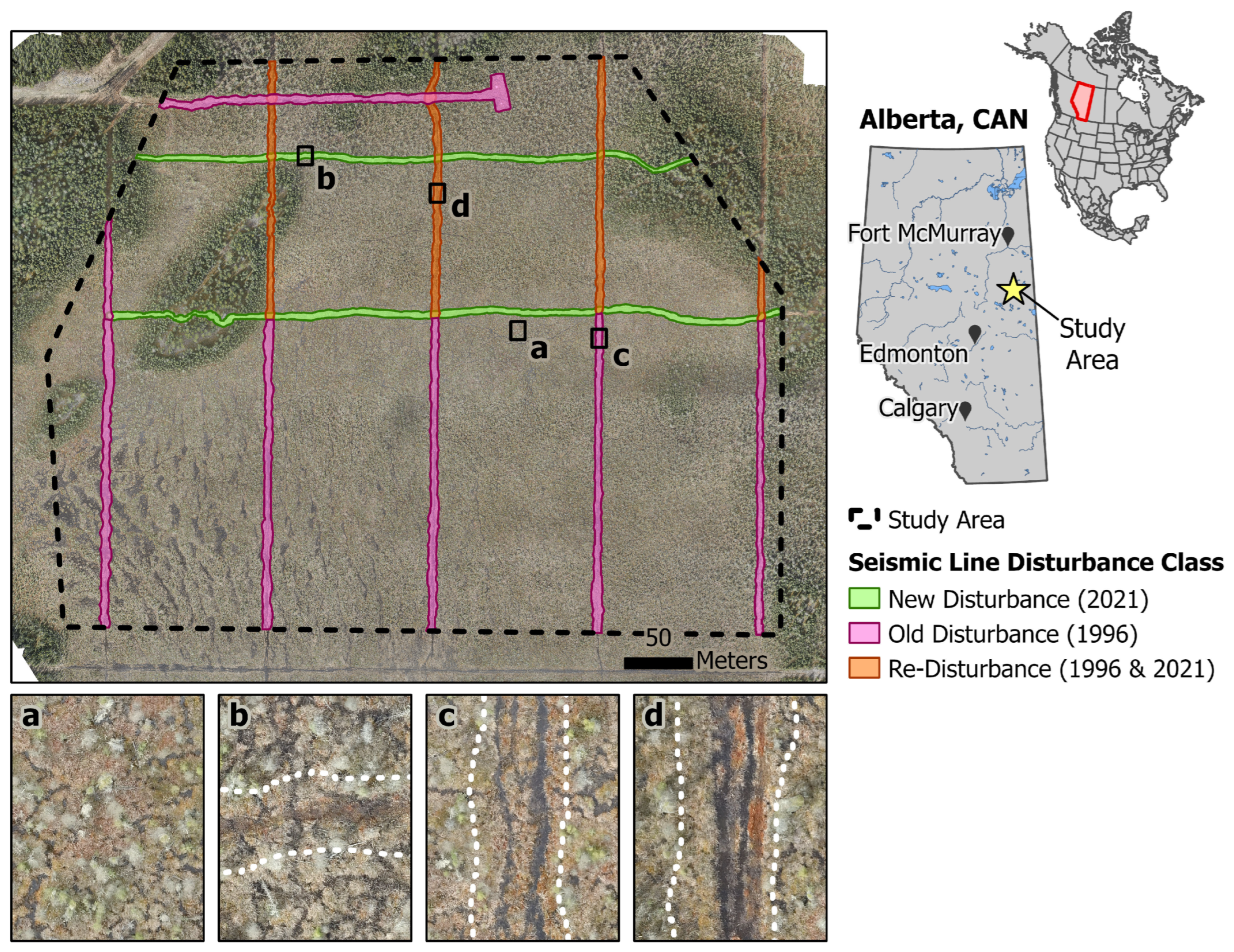
The study area is a 20-hectare portion of a fen, located approximately 150 km south of Fort McMurray, Alberta (Figure 1). It is situated within the central mixed-wood subregion of the boreal forest, and is characterized by a mixture of uplands and wetlands, including bogs, fens, marshes, and swamps [41]. This area has a continental subarctic climate characterized by cold winters and short, warm summers. Common woody vegetation found in the study area includes black spruce (Picea mariana (Mill.) Britton, Sterns & Poggenb.), tamarack (Larix laricina (Du Roi) K. Koch), bog birch (Betula glandulosa Michx.), and bog willow (Salix pedicellaris Pursh). The trees are sparse and often do not exceed 3 m in height, resulting in no closed canopy found in the study area. Common herbaceous vegetation includes buckbean (Menyanthes trifoliata L.), water sedge (Carex aqutilis Wahlenb.), and horsetail (Equisetum fluviatile L.). The study area is carpeted by various species of moss, such as fine bog moss (Sphagnum angustifolium (Warnst.) C.E.O. Jensen), rusty bog moss (Sphagnum fuscum (Schimp.) H. Klinggr.), and tufted moss (Aulacomnium palustre (Hedw.) Schwägr.), which form hummock-hollow complexes. The water table is shallow and there are natural pockets of surface water throughout the study area.
There are numerous resource extraction activities and associated anthropogenic disturbances in the study area and surrounding region, including roads, well pads, pipelines, oil sands extraction infrastructure, and seismic lines. The study area is dissected by a dense network of LIS lines ranging from 2–4 m in width, totaling 3.1 km in length. These lines were likely created using a drum mulcher or narrow bulldozer, which we categorized into three disturbance classes:
  • New disturbance: Seismic lines newly created in 2021 (1 year old at the time of data collection).
  • Old disturbance: Seismic lines created in 1996 (26 years old at the time of data collection).
  • Re-disturbance: Seismic lines originally created in 1996 and re-cleared for additional seismic surveying during the 2021 campaign.
The age and history of individual lines were verified in the field by locating shot tags, which are small aluminum markers attached to some trees along seismic lines. Each tag records permit and program information from the seismic survey that created it. The presence of shot tags with different years along the same corridor confirmed cases of re-disturbance.
This study design follows a space-for-time substitution (chronosequence), where differences among disturbance classes are interpreted as representing stages of recovery over time. Within this framework, the matrix (undisturbed area adjacent to the lines) represents the expected peatland attributes before a seismic line is created. The new disturbance illustrates peatland attributes shortly after a seismic line is created. Over time, these attributes fluctuate and change due to factors like inundation or vegetation regrowth, eventually resembling the attributes found in the old disturbances. Finally, these altered attributes are modified once more by repeated seismic surveys. This approach assumes that sites are comparable aside from disturbance history; however, unmeasured differences in site conditions may influence observed patterns and should be considered when interpreting results.

2.2. RPAS Data Collection

RPAS-based LiDAR and true-colour imagery were collected in May 2022. LiDAR was collected using a DJI Zenmuse L1 sensor (DJI, Shenzhen, China) aboard a DJI Matrice 300 RTK (DJI, Shenzhen, China). The sensor was flown approximately 100 m above ground level with triple-return mode and repetitive scanning enabled at a sampling rate of 160 kHz. The L1 sensor uses a near-infrared laser (905 nm), and the final point cloud had a density of 185 points/m2. We performed a variety of post-processing steps (e.g., noise removal, ground classification) on the point cloud using LAStools (version 190221; rapidlasso GmbH, Gilching, Germany) [42]. We then generated a 10 cm digital terrain model (DTM) from the classified ground points using a k-nearest neighbor inverse-distance weighted algorithm (knnidw; k = 10, p = 2) in the R package lidR (R version 4.1.3; R Foundation for Statistical Computing, Vienna, Austria) [43,44]. We used the same package to produce a 10 cm canopy height model (CHM) by first subtracting the DTM from the point cloud (i.e., normalizing the point cloud height), then rasterizing the resultant point cloud by height.
A spatially and temporally coincident optical dataset was collected using a DJI Zenmuse P1 sensor (DJI, Shenzhen, China) (full-frame 45-megapixel camera with a 35 mm lens) on the same RPAS used to collect the LiDAR. We flew approximately 110 m above ground level. The side and front overlap were set to 70% and 80%, respectively. This imagery was processed into a 2 cm resolution true-colour orthomosaic using Pix4Dmapper (version 4.8.0; Pix4D SA, Prilly, Switzerland) [45]. Refer to Appendix A for details on georeferencing and accuracy assessment of the RPAS data.

2.3. Classifying Microforms

The DTM was used to derive rasters of microforms (i.e., hummocks, lawns, and hollows) by adapting the methods presented in Lovitt et al. [37]. First, a smoothed DTM was created by computing the focal mean of each pixel in the original DTM using a 3 m moving window. The smoothed DTM was then subtracted from the original DTM, resulting in a detrended DTM that depicts elevation deviation from the local average. In this raster, positive values represent locations where the elevation is greater than the local 3 m average, whereas negative values are locations with elevations less than the local 3 m average. We re-classified this raster into three microform categories: hummocks (elevation more than 6 cm higher than the local 3 m average), lawns (elevation within ± 6 cm of the local 3 m average), and hollows (elevation more than 6 cm below the local 3 m average). The 6 cm threshold was selected because it produced microform maps that were visually consistent with observed field microforms in this fen. The result is a 10 cm resolution raster of microforms. We explored threshold values ranging from 5 to 15 cm and found that while absolute hummock cover values varied with threshold choice, the relative differences among disturbance classes remained consistent, supporting the robustness of this approach.

2.4. Estimating DTW

The DTW raster was derived by adapting the methods presented in Rahman et al. [30]. Their workflow takes advantage of the abundant small water bodies that are characteristic of peatlands, generally consisting of puddle-sized pools occurring every few meters across the surface. Given that surface water is tightly linked to groundwater in peatlands, Rahman et al. [30] found that an accurate water table surface can be generated by interpolating the elevation of visible water bodies. Once a water table surface exists, this layer simply needs to be subtracted from the DTM to produce estimates of DTW. However, this approach assumes that the elevation of surface water bodies approximates the local groundwater level. While this assumption is generally supported in peatland systems due to strong hydrological connectivity, it was not directly validated with field measurements in this study and therefore introduces uncertainty into the DTW estimates.
This approach begins with supervised classification of surface water pixels in the true-colour orthomosaic. First, the CHM is used to mask the true-colour orthomosaic such that pixels with a canopy height > 0.2 m cannot be considered water. Using the true-colour orthomosaic as reference, we manually digitized polygons that contained either surface water (n = 91), ground (n = 139), or shadowed ground (n = 81). Within each polygon, two random points were generated to become training sites. RGB values from the true-colour orthomosaic were extracted for all training sites, then we used a recursive partitioning decision tree method from the R package rpart [46] to train the classifier. This classifier was applied to the true-colour orthomosaic for the entire study area to identify bodies of surface water. A filter was applied to remove clumps of water pixels that were less than 20 × 20 cm. A 5-fold cross-validation based on the training dataset yielded an overall classification accuracy of 84%, indicating that surface water features were reasonably well distinguished from other classes.
The surface water raster was used to mask the DTM, resulting in a raster that contained only elevation values for surface water pixels. A 10 × 10 m grid was created over the study area, and the minimum water elevation value was assigned to the centroid of each grid cell. This choice was made based on comparison with GNSS-derived surface water elevations (Appendix A), where using the minimum value resulted in the lowest root mean square error (RMSE) relative to field observations. Grid cells that visibly contained no surface water were removed. The remaining centroids were used to interpolate a water table surface using ordinary kriging. The R package gstat was used to fit the semivariogram model (model = Matern (M. Stein’s parameterization), partial sill = 0.865, range = 2783.461) and to perform the ordinary kriging onto a 10 cm resolution grid (matching the DTM grid) using 10 nearest observations [47,48]. The upland knoll in the northwest portion of the study area was masked out because the water table estimation would be poor here due to a lack of surface water bodies.
The water table raster was subtracted from the DTM, resulting in a 10 cm resolution DTW product. In this product, positive values represent the distance of the water table below the ground surface, and the minimum possible value is 0, representing surface water. In addition, all pixels labelled as surface water from the supervised classification were also forced to have a value of 0. Conceptually, it would be expected that a pool of water has a negative DTW, i.e., the water itself has depth that overlies the ground surface. However, due to limitations of near-infrared LiDAR, we are unable to model the ground surface that underlies pools of water, and thus DTW = 0 is the minimum value for this study. This represents a methodological limitation, as the truncation of DTW at 0 prevents characterization of water depth above the ground surface and may lead to underestimation of hydrological variability in areas with standing water.

2.5. Comparing Disturbance Types

The Forest Line Mapper (version 1.2; Applied Geospatial Research Group, University of Calgary, Calgary, AB, Canada) [49] is a semi-automated software tool for mapping linear features in forests using a CHM as input. We used this tool to map the centerline of seismic lines in the study area. We mapped 0.93 km, 1.5 km, and 0.62 km of seismic lines in the new disturbance, old disturbance, and re-disturbance classes, respectively. Polygon segments were created along the centerlines to act as aggregation units for the comparison analysis. These segments measure 1 × 10 m. Each seismic line segment is associated with two additional 1 × 10 m segments, located 15 m into either side of the adjacent matrix. These matrix segments are assumed to approximate the baseline conditions on the associated seismic line segment. Together, the three segments (one on seismic line, two within matrix) can be considered a segment set. Segment sets that were considered not representative of the fen, such as the segments that intersect the upland knoll in the northwest portion of the study area, were removed prior to further analysis. In total, there were 267 segment sets (n new disturbance = 70, n old disturbance = 144, n re-disturbance = 53).
The data products of interest (elevation, hummock proportion, surface water, DTW) were summarized within the seismic line and matrix segments (see column “Method of aggregation”, Table 1). Basic summary statistics (e.g., mean, median, range, variance) were computed for all segments. Where appropriate, deviation of variables between seismic line segments and adjacent matrix segments were calculated as differences. All computed metrics are shown in Table 1.
Kruskal–Wallis rank sum tests and pairwise Wilcoxon rank sum tests with Benjamini–Hochberg (BH) correction were used to evaluate whether deviation metrics differed between the seismic line disturbance types (new disturbance, old disturbance, re-disturbance). Non-parametric tests were selected as the deviation metrics violated assumptions of normality and equal variance required for parametric analyses. Because disturbance effects may manifest not only as shifts in central tendency but also as changes in variability, both mean-based and variance-based tests were used to provide a more comprehensive assessment of differences among disturbance types. Therefore, we additionally implemented the Brown–Forsythe test for equality of variances (a robust Levene-type test using group medians), followed by pairwise Brown–Forsythe comparisons with BH correction. Unequal sample sizes among disturbance classes were present due to differences in available seismic line length; however, the use of non-parametric tests and variance-based methods reduces sensitivity to unequal group sizes and variance heterogeneity.

3. Results

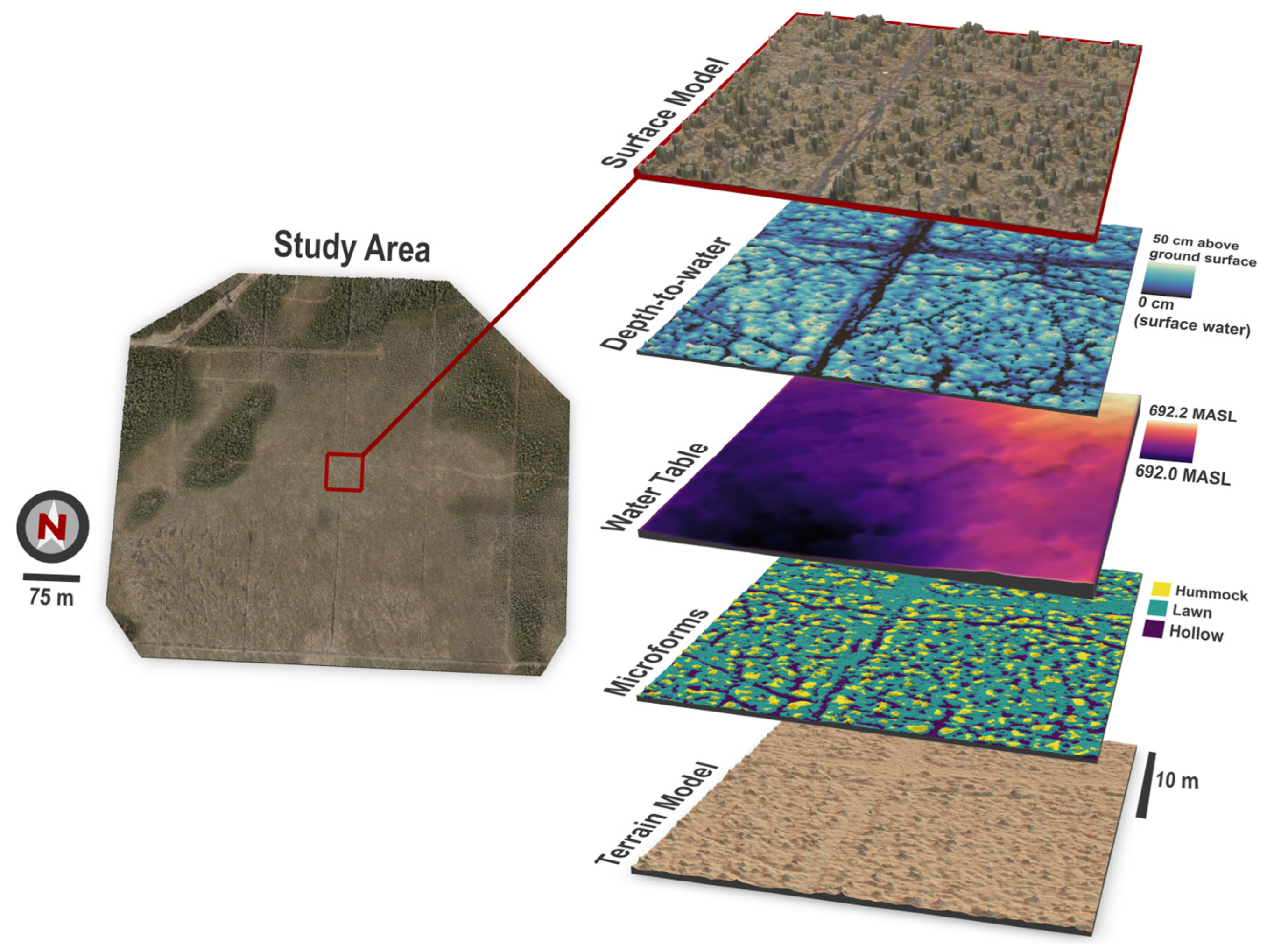
We used RPAS to characterize surface morphology and hydrology variables in a boreal fen that has been subjected to repeated seismic surveys. A selection of the mapped variables is shown in Figure 2.

3.1. Elevation Deviation

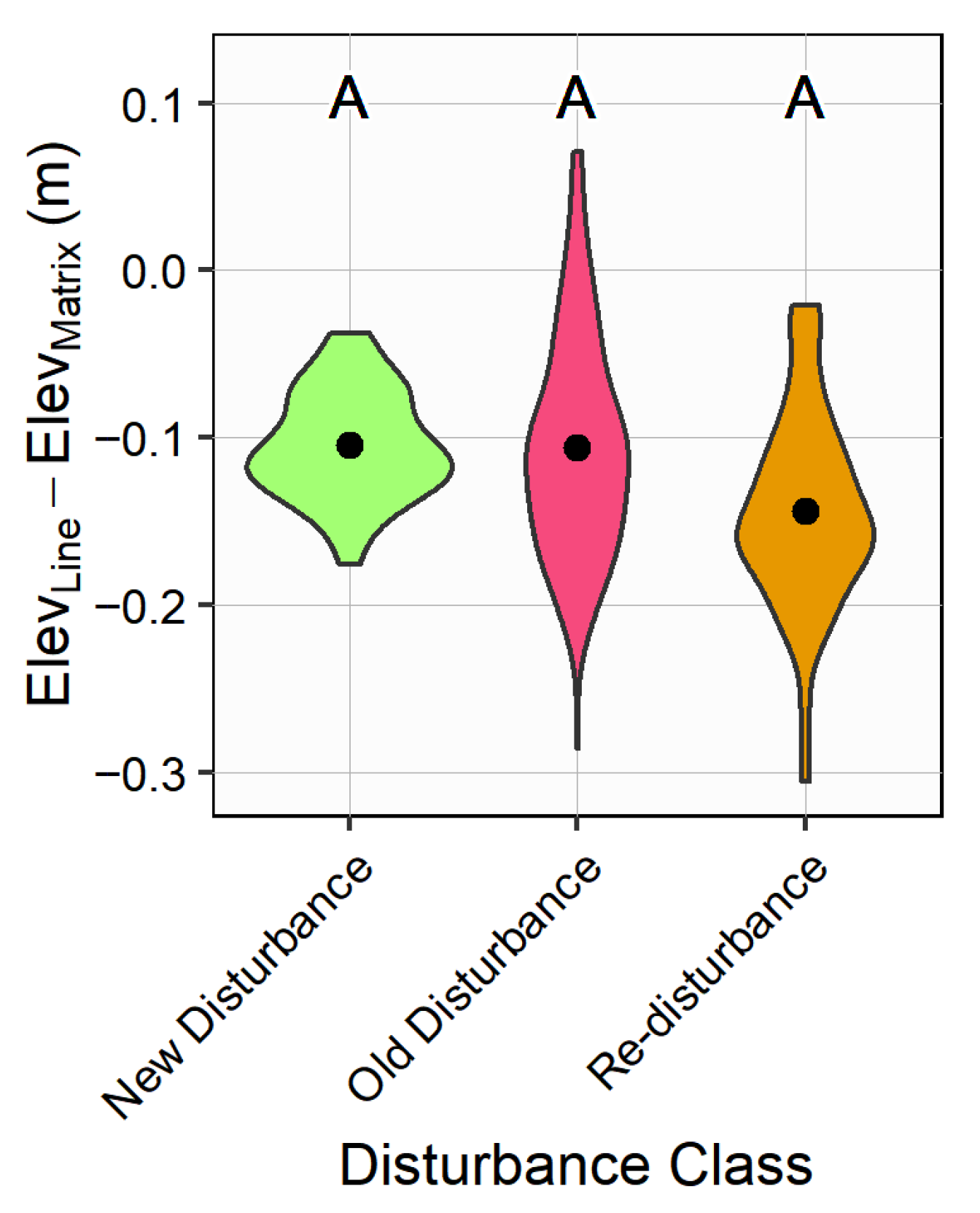
Seismic lines tended to be depressed relative to the adjacent matrix. On average, new disturbances, old disturbances, and re-disturbances were depressed compared to the adjacent matrix by 10 cm, 11 cm, and 14 cm, respectively (Figure 3, Table 2). We did not observe significant differences in elevation deviation among the disturbance classes (Kruskal–Wallis test, χ2(2) = 4.8, p = 0.87). However, variance differed significantly among classes (Brown–Forsythe test, F(2, 169.21) = 11.54, p < 0.001). Pairwise Brown–Forsythe comparisons showed that new disturbances had significantly lower variance than both old disturbances (p = 0.00025) and re-disturbances (p = 0.00007), while old disturbances and re-disturbances did not differ (p = 0.78) (Table 2). Although old disturbances and re-disturbances had similar overall variance, the re-disturbances lacked the higher-elevation tail present on old disturbances, suggesting that the distribution of surface conditions differs qualitatively between these two classes beyond what variance statistics alone capture (Figure 3).

3.2. Hummock Proportion & Deviation

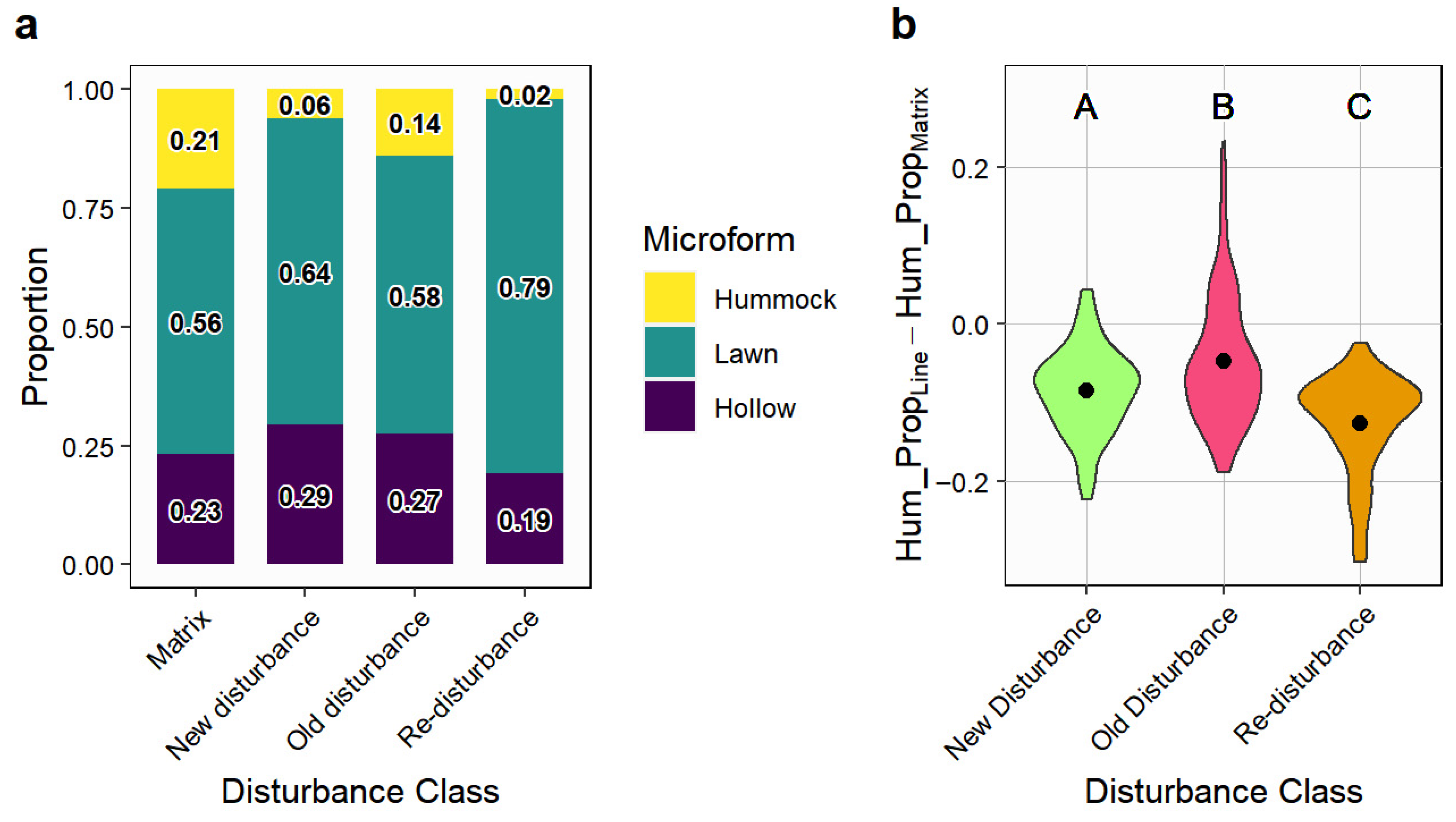
The ground surface in the matrix had a higher proportion of hummocks compared to seismic lines. Whereas hummocks covered 21% of the matrix segments, they covered only 6%, 14%, and 2% of segments along new disturbances, old disturbances, and re-disturbances, respectively (Figure 4a).
There were significant differences in the mean hummock proportion deviation between all disturbance classes (Pairwise Wilcoxon test, all p < 0.01). On average, segments on old disturbances had an absolute difference of 5% less hummock cover compared to adjacent matrix segments, whereas new disturbances and re-disturbances averaged 8% less and 13% less, respectively (Table 3, Figure 4). Compared to adjacent matrix segments, this represents an average relative decrease of 30%, 67%, and 90% in hummock cover on old disturbances, new disturbances, and re-disturbances, respectively. Variance in hummock proportion deviation also differed significantly between disturbance classes (Brown–Forsythe test, F(2, 179.92) = 27.36, p < 0.001). Pairwise Brown–Forsythe tests showed that old disturbances exhibited significantly greater variance than both new disturbances (p = 0.00004) and re-disturbances (p = 2.8 × 10⁻⁹), while new disturbances and re-disturbances also differed significantly (p = 0.00002), though the magnitude of this difference was small (Table 3).

3.3. Surface Water Proportion & Deviation

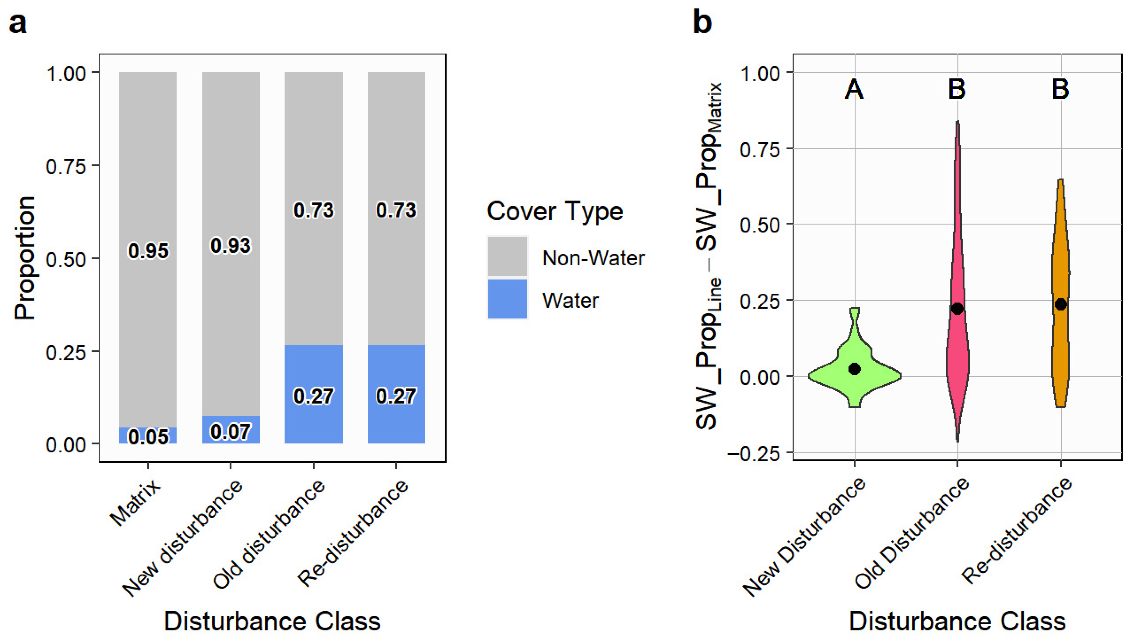
Surface water covered a greater proportion of segments on old disturbances and re-disturbances compared to the matrix and new disturbances. Whereas surface water covered 5% and 7% of segments on the matrix and new disturbances, respectively, segments on old disturbances and re-disturbances were 27% surface water (Figure 5a).
The mean surface water deviation on new disturbances (mean = 2%) was significantly less than on old disturbances (mean = 22%; Pairwise Wilcoxon test, p < 0.01) and re-disturbances (mean = 24%; Pairwise Wilcoxon test, p < 0.01). There was no significant difference in the mean surface water deviation between old disturbances and re-disturbances (Pairwise Wilcoxon test, p = 0.42). Variance also differed significantly among classes (Brown–Forsythe test, F(2, 105.80) = 8.67, p < 0.001). Pairwise Brown–Forsythe comparisons showed that variance on new disturbances was significantly lower than both old disturbances (p = 3.5 × 10⁻⁶) and re-disturbances (p = 0.00137), whereas old disturbances and re-disturbances showed no difference in variance (p = 0.75) (Table 4).

3.4. Depth-to-Water Deviation

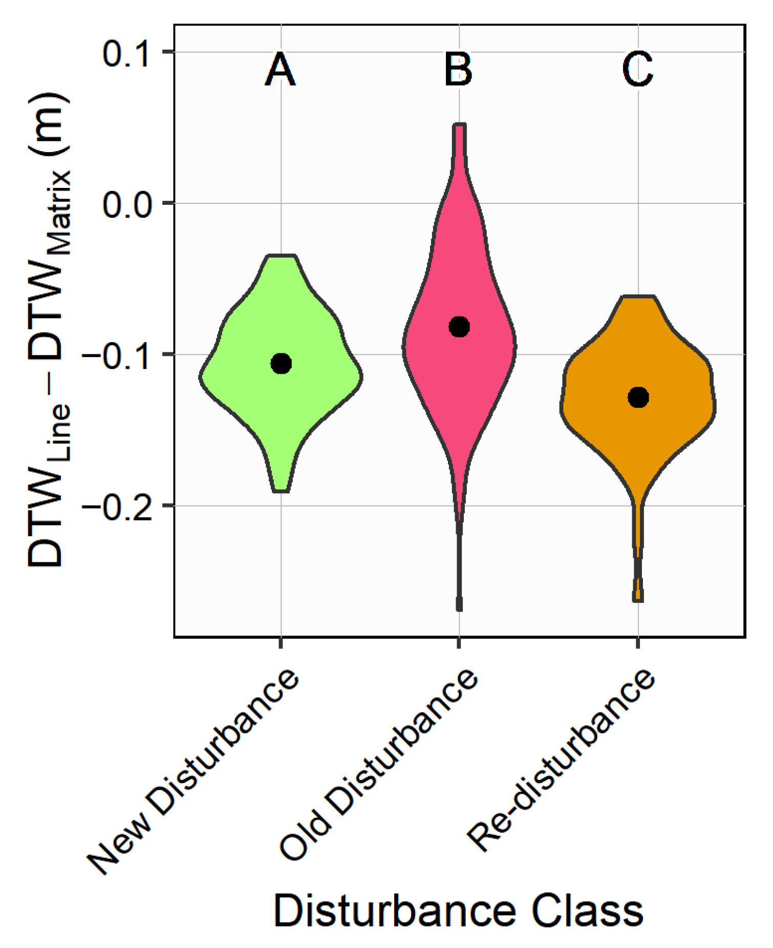
Seismic lines tended to have shallower (i.e., closer to the ground surface) DTW than the adjacent matrix. On average, new disturbances, old disturbances, and re-disturbances had water tables that were shallower than the adjacent matrix by 11 cm, 8 cm, and 13 cm, respectively (Figure 6, Table 5). Significant differences in mean DTW deviation were observed among all disturbance classes (Pairwise Wilcoxon test, all p < 0.01). Variance also differed significantly among classes (Brown–Forsythe test, F(2, 233.61) = 28.35, p < 0.001). Pairwise Brown–Forsythe comparisons indicated that old disturbances had significantly greater variance than both new disturbances (p = 0.00013) and re-disturbances (p = 3.9 × 10⁻¹⁰), whereas new disturbances and re-disturbances also differed, with higher variance on re-disturbances (p = 0.00062) (Table 5).

4. Discussion

These interpretations are based on observations from a single 20-hectare boreal fen and should therefore be interpreted within the context of this case study. This study revealed distinct differences in surface morphology and hydrology among seismic lines with different disturbance histories. New disturbances showed relatively uniform depression and limited microtopographic variability, reflecting the immediate effects of compaction and vegetation removal. Old disturbances displayed greater variability, with evidence of both microtopographic recovery and continued degradation, indicating divergent recovery trajectories over time. In contrast, re-disturbances are consistent with a resetting of surface structure, with partially recovered hummocks appearing to have been removed and conditions resembling or exceeding the degradation observed immediately after initial disturbance. These findings suggest that repeated seismic surveys in this study site amplified the alteration of peatland surface morphology and hydrology, setting back the process of natural recovery.
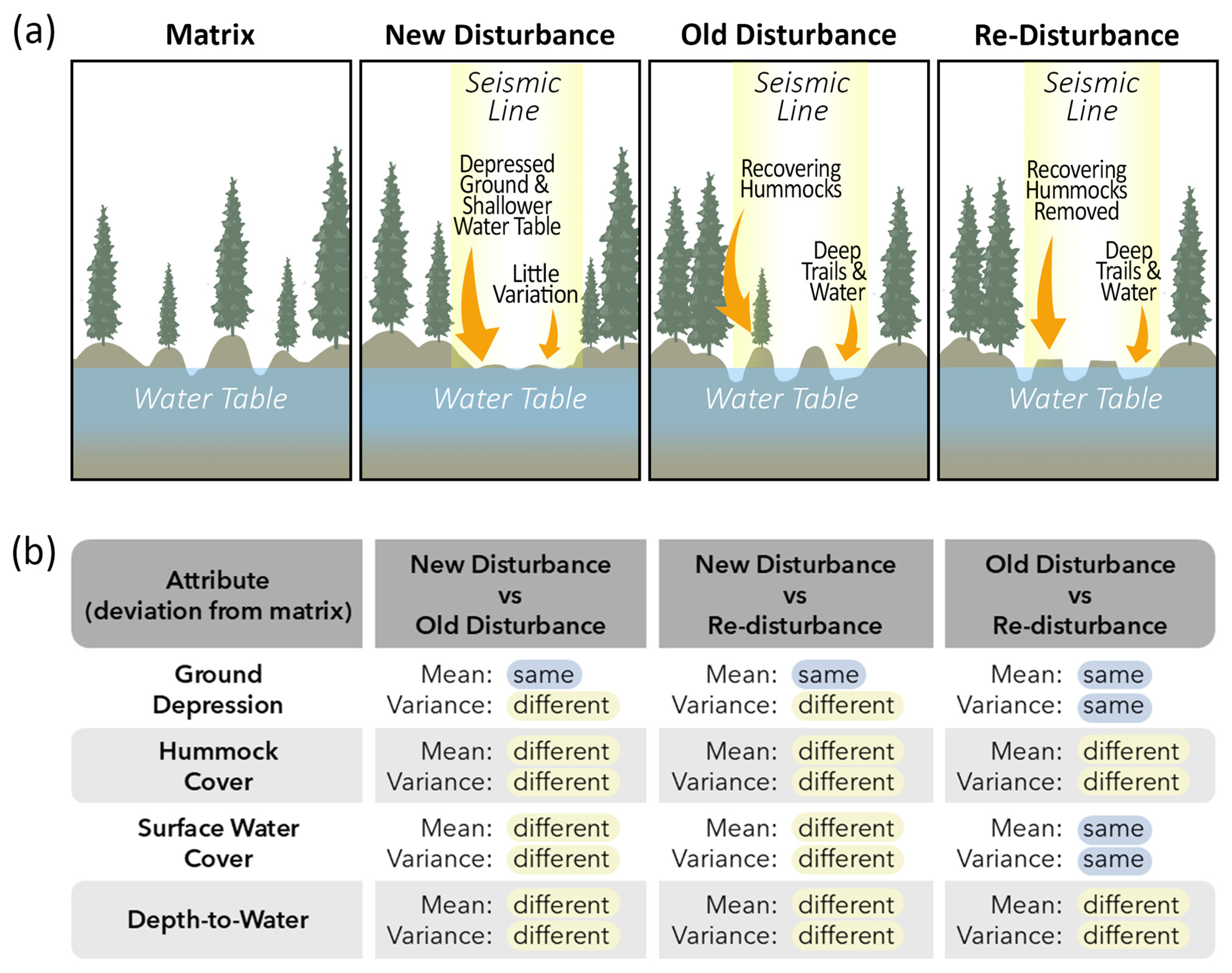
To contextualize these patterns and provide a foundation for the discussion that follows, Figure 7 synthesizes the major microtopographic and hydrological responses observed across the three disturbance classes. Panel (a) presents a conceptual schematic illustrating how initial disturbance, recovery over time, and subsequent re-disturbance shape surface morphology and hydrology. Panel (b) complements this by summarizing the statistical outcomes of all pairwise comparisons of means and variances for the four key attributes examined in this study: ground depression, hummock cover, surface water cover, and DTW. In the sections that follow, we interpret these patterns in detail and discuss their implications for understanding peatland recovery and managing seismic lines.

4.1. Progression of Peatland Properties Following Disturbance

The disturbance classes in this study offer insights into how disturbance and recovery influence the progression of peatland properties. Below, the matrix and seismic line disturbance classes are discussed in the order that conceptualizes surface morphology and hydrology evolution over time.
Matrix: The matrix represents the expected natural peatland condition in the absence of disturbance, providing a benchmark against which seismic line conditions are interpreted. The relatively high hummock cover, limited surface water, and deeper DTW observed in the matrix reflect conditions that support the establishment of sparsely distributed black spruce and tamarack.
New disturbances: The new disturbances were created in 2021 and represent seismic line properties one year after a single disturbance. Although they offer insight into early post-disturbance conditions, differences in survey methods between 1996 and 2021 must be considered. Earlier lines were generally wider and constructed with heavier machinery that caused greater compression and vegetation removal. Consequently, the new lines may not directly represent the initial state of the old disturbances but instead provide a comparative baseline for understanding how disturbance practices influence subsequent recovery.
The new disturbances were on average depressed 10 cm compared to the baseline surface of the matrix, and the distribution of the line depression fell within a relatively limited range (min = −18 cm, max = −4 cm). This magnitude of ground depression is consistent with previous observations that seismic lines typically sit 1–8 cm below the adjacent treed peatland surface [18,50] and falls within the range of compaction effects observed by Pinzon et al. [29]. Such compaction has ecological consequences, as even small reductions in surface elevation can lead to shallower DTW and increase soil moisture in peatlands with shallow hydrology [19,29]. The variance in elevation deviation on new disturbances was also significantly lower than on both old disturbances and re-disturbances, indicating a more uniform expression of ground compression in the first year after disturbance. The proportion of hummock cover on new disturbances was considerably reduced compared to the matrix; there was an average relative decrease of 30%. This flattening of microtopography is consistent with previous findings that seismic line construction reduces microtopographic complexity by 20% [18]. However, this may be the result of specific parameters utilized in creating seismic lines in this area. In the field, we observed that hummocks on these seismic lines appeared to have their tops “sliced” off, likely at the set drum height of the mulcher. This resulted in a seismic line with minimal microtopographic variation, but the bottoms of hummocks remained intact. Had the drum of the mulcher been raised higher, we may have observed better preservation of the microtopography. Operational parameters during line creation can directly affect the degree of surface disturbance, with implications for both the preservation of hummock structure and subsequent vegetation recovery [51,52].
Despite the line depression, we observed very similar proportions of surface water on the new disturbances (7%) compared to the matrix (5%). Indeed, in the field we observed that new disturbances appeared depressed and very flat (i.e., few hummocks), but lacked pooling water as witnessed on other disturbance classes. This absence of surface pooling may reflect both the short time since disturbance and the lower weight equipment used during modern surveys, which likely caused less soil compression. Together, these factors suggest that visible pooling may not develop until several years after the disturbance, as discussed further for the old disturbances below. The DTW was shallower on average by 11 cm compared to the matrix, and this shift was fairly uniform; the variance in DTW deviation on new disturbances was significantly lower than on both old and re-disturbances. The progression to a shallower DTW can be attributed to the reduction in the ground elevation, stemming both from line depression and hummock damage, consistent with Lovitt et al. [50], who reported a 15 cm decrease in mean DTW along LIS lines compared to adjacent peatland.
Old disturbances: The old disturbances were created in 1996, and, at the time of sampling, represented seismic line properties 26 years after a single disturbance. They are expected to reasonably depict how the new disturbances might appear after ~26 years. These seismic lines were not significantly more depressed compared to the new disturbances, which suggests that the average compression remains constant over time. Prior studies have found that seismic line depression can persist for decades due to feedbacks between reduced vegetation recovery, shallower water tables, and inhibited Sphagnum establishment, which collectively delay microtopographic recovery [18,50]. However, Figure 3 shows that the distribution of elevation deviation differs considerably from the new disturbances. While the mean elevation deviation is similar, old disturbances exhibit substantially greater variability—from −29 cm to +7 cm—compared to the narrower range observed on new disturbances. This broader spread is consistent with our Brown–Forsythe results, which indicate significantly higher elevation variance on old disturbances. Together, these patterns suggest diverging microtopographic trajectories over time. In other words, the distribution of elevation deviation becomes more extreme (in both positive and negative directions) over the span of 26 years. In the positive direction, we interpret this to depict microtopography recovery over time; some areas (where elevation deviation > 0) even suggest that microtopography has recovered to the level of the matrix over 26 years. This is corroborated by Figure 4, which shows that hummocks comprise a greater proportion of the ground cover and deviate less from than matrix on old disturbances compared to new disturbances. The greater variance in hummock proportion on old disturbances relative to new disturbances further supports this pattern, indicating mixed states of degradation and recovery. Field observations also revealed hummocks supporting regenerating vegetation, including seedlings and small trees (<1 m tall), on these lines.
In the negative direction, we interpret this as some areas experiencing further degradation of the ground surface over time. While natural hollows are present in peatlands, the magnitude of the negative elevation deviations on old disturbances exceeds that observed on new disturbances, suggesting that these depressions are not solely the result of inherent microtopographic variation. One explanation for this could be trampling by wildlife. Seismic lines are known to act as animal movement corridors; they have a funneling effect on the movement patterns of some animals [14]. Similarly, Pinzon et al. [29] observed trails along seismic lines that likely contributed to surface variability and reshaped the ground surface. McDermid et al. [17] mapped trails and tracks in the same region as our study area and found that the density of trails and tracks is 4.4-times greater on seismic lines compared to the matrix. Field observations corroborated this pattern, showing dense networks of animal trails on seismic lines, while only sparse trail features were evident in the surrounding matrix. While this study did not directly measure animal activity or movement, we suggest that the use of seismic lines as animal movement corridors over the past 26 years may have contributed to additional ground degradation in some portions of these features. This may also partially explain why the proportion of surface water increases from 7% on new disturbances to 27% on old disturbances; we observed that water pooled into the animal trails, contributing considerably towards the surface water cover. Such localized inundation has been identified as a key mechanism reinforcing long-term depression and delayed vegetation recovery on seismic lines [18]. The mean DTW on old disturbances was significantly less shallow than the new disturbances, but similar to elevation deviation, the variance in DTW deviation was also significantly higher on old disturbances. These findings indicate that, over time, spatial heterogeneity has increased on old disturbances, with some areas exhibiting microtopographic recovery and others experiencing continued surface degradation.
Re-disturbances: The re-disturbances were initially created in 1996, then re-disturbed in 2021, representing seismic line properties after two disturbances. They are expected to reasonably depict how the old disturbances would appear if they were re-disturbed. Elevation deviation was not significantly different compared to the old disturbances, but the distribution of values shifted lower, suggesting that the second disturbance removed portions of the microtopography that had partially recovered over the preceding decades. Variance in elevation deviation did not differ between old disturbances and re-disturbances, indicating that although the second disturbance shifted the mean downward, it did not introduce additional heterogeneity beyond that already present on the old disturbances. This is corroborated by the hummock proportion analysis, which shows that the re-visit reduces the overall hummock cover from 14% down to 2%; in addition, re-disturbances have an average relative decrease of 90% compared to the matrix (Figure 4). The hummock proportion, and by extension, the amount of suitable seedling sites, decreases dramatically after a re-visit, even dropping below the conditions observed immediately after seismic line creation (i.e., the new disturbance). Similar observations have been made for winter roads constructed along pre-existing linear features, where repeated use and heavy machinery traffic further compacted the peat, increased surface wetness, and altered vegetation composition [21].
The proportion of surface water did not change between old disturbances and re-disturbances (both 27% surface water). However, we collected data just one year after the re-visit, and considering the tendency for water to pool in animal trails, there might be a lagged effect that will appear with more time. DTW was significantly worse than both new and old disturbances, suggesting the high degree of surface disturbance resulting from the re-visit.

4.2. Implications for Recovery & Management

Overall, the results of this study illustrate the interplay between disturbance and recovery over time following repeated seismic surveys. After the initial compression of the peatland surface, some areas begin to recover microtopography while others continue to degrade, creating greater variability over time. When a subsequent re-disturbance appears to reset this process, hummocks that had developed since the initial disturbance may have been removed. This pattern highlights how repeated disturbance reinforces long-term alterations to surface morphology and hydrology, ultimately delaying peatland recovery.
Seismic line recovery can be defined in several ways, depending on management priorities. In Alberta’s boreal region, recovery initiatives have largely been driven by the need to reduce predator movement along seismic lines to support woodland caribou conservation [3,10,11]. From this perspective, recovery may be achieved once vegetation regenerates sufficiently to limit predator line-of-sight and impede movement [14]. However, ecosystem recovery extends beyond vegetation regeneration—it also requires the restoration of ecological functions that depend on the re-establishment of microtopography. Microtopography plays a central role in regulating water-table position, surface wetness, and the availability of microsites for vegetation establishment [18,53] and should be recognized as a key component of peatland recovery.
These findings also challenge the assumption that LIS lines are low impact. Although LIS lines are narrower and designed to minimize ground disturbance [3], our data suggest that, at least within the context of this case study, even a single pass of machinery may substantially reduce microtopographic variability and flatten hummocks. Re-disturbance exacerbates this effect, removing partially recovered microforms and promoting surface wetness that inhibits regeneration. Thus, while LIS lines are intended to reduce environmental footprint, their long-term effect may include persistent hydrological alteration and reduced recovery potential, particularly when they are re-used.
A central management question emerging from these results is whether it is preferable to re-use existing lines or to construct new ones. Re-use avoids increasing the total linear footprint but can intensify degradation within already compacted peat, whereas new lines expand the overall disturbance area but may leave partially recovered sites intact. Given the slow pace of natural recovery and the compounding effects of re-disturbance observed here, the relative trade-offs likely depend on ecosite type, vegetation composition, and the degree of prior compression. While matrix segments were used to approximate undisturbed peatland conditions, it is possible that broader landscape disturbances or legacy effects may also influence these areas. This study cannot directly determine which option minimizes cumulative impact, as doing so would require pre-disturbance data, direct comparisons between re-used and newly cut lines, and replication across multiple sites and peatland types. The trade-off discussion presented here is therefore intended to frame an important management question rather than to resolve it, and should be interpreted as conceptual rather than evidence-based guidance.
From a management perspective, these results emphasize the need to assess the condition of seismic lines before re-use or restoration decisions are made. Lines with partial microtopographic recovery and limited surface wetness may be on a natural recovery trajectory and should be protected from further disturbance. In contrast, lines exhibiting persistent depression, high surface water cover, or evidence of intensive trail formation may require active intervention to restore microtopography and subsequent ecosystem functions. Integrating microtopographic assessment into monitoring frameworks would provide a more mechanistic indicator of recovery trajectory, allowing managers to tailor restoration approaches to site-specific conditions.

4.3. Limitations & Future Directions

This case study examined three disturbance classes within a single fen, providing detailed insights but limiting broader inference. Fens are the dominant peatland type in northern Alberta, yet they vary widely in hydrology and vegetation depending on local topography and groundwater inputs [54]. As such, results may not represent other ecosite types or regional conditions. Expanding analyses across multiple sites and peatland types would help test the generality of these patterns. Differences in seismic line orientation also introduce uncertainty. The new disturbances were oriented east–west, whereas old disturbances and re-disturbances were mostly north–south. Orientation influences solar radiation, evapotranspiration, and potentially groundwater flow [55], which may affect surface wetness and hummock recovery.
A further limitation is that both the new disturbances (2021) and re-disturbances (2021) were likely created by a single operator using the same machine during the winter seismic program. The mulcher drum height and operator judgment strongly influence the degree of surface disturbance. Field observations suggested that the mulcher drum may have been set relatively low, “slicing” the tops off hummocks while leaving their bases intact. This introduces uncertainty about how representative these conditions are of other seismic programs, operators, or equipment configurations. Because this study captures one snapshot of a single repeated survey conducted by one operator, caution is needed when extrapolating these results to LIS practices.
Several analytical choices introduce additional uncertainty. First, hummocks were identified using a threshold of 6 cm above a 3 m moving-window mean elevation. Although this threshold produced classifications consistent with field interpretation, alternative thresholds (e.g., 5–15 cm; different window sizes) would alter hummock proportions and may affect estimated differences among disturbance classes. Future work should evaluate whether this elevation-deviation threshold aligns with field-measured microtopographic structure (e.g., measured hummock–lawn height differences), and refine threshold selection accordingly. Second, DTW was modelled by interpolating groundwater surfaces from pockets of standing water, assuming close coupling between surface water and the water table. While this approach is supported by prior peatland hydrology studies, deviations from this assumption may introduce error. Direct validation of these estimated DTW surfaces using water-table measurements between surface-water features (e.g., using wells) would strengthen confidence in the method. Third, sample sizes differed among disturbance classes (e.g., n = 70 new disturbance segments versus 144 old disturbance segments), which may influence statistical power. Additionally, attributes such as line depression and water pooling may reflect both disturbance history and line orientation, making it difficult to fully disentangle compositional from directional effects. Finally, segments along the same seismic line are likely to exhibit spatial autocorrelation, which may affect the independence assumption underlying the nonparametric statistical comparisons. While this could produce overly optimistic p-values by inflating effective sample size, it does not bias the point estimates themselves. Given the magnitude of the differences observed among disturbance classes, we are confident this does not alter the substantive conclusions of the study. While none of these assumptions undermine the overall patterns observed in this study, they introduce uncertainty that should be addressed through future multi-site, multi-year analyses.
A key management question arising from this work is whether re-using existing seismic lines is truly a lower impact strategy compared to cutting new lines. This study cannot definitively answer that question, because it lacks pre-disturbance data. A more robust evaluation would require time-series data spanning: (1) pre-disturbance conditions, (2) immediately post-disturbance, (3) decades of recovery, and (4) conditions immediately after re-disturbance, and beyond. Such a design would allow quantification of the incremental effect of repeated disturbance relative to both initial impact and recovery trajectory. Importantly, the determination of whether re-use is preferable depends on management goals. Resolving this requires explicit definitions of both the desired outcomes and the assessment criteria of recovery. Future work integrating physical, vegetation, and carbon metrics—and monitoring recovery rates under both strategies—will be essential for providing evidence-based guidance on this trade-off.

5. Conclusions

This study examined how peatland surface morphology and hydrology vary across seismic lines with different disturbance histories, using high-resolution RPAS-based LiDAR and optical imagery. To our knowledge, this represents the first application of RPAS-derived LiDAR and optical imagery to explicitly examine the cumulative effects of repeated seismic disturbance on peatland surface conditions, providing new empirical evidence on a management practice whose ecological consequences have remained poorly understood. By assessing new seismic lines, old seismic lines, and re-disturbances relative to adjacent undisturbed peatland, we addressed two research objectives.
First, we sought to quantify differences in microtopography and hydrology among disturbance classes and undisturbed peatland. Each disturbance class exhibited distinct surface conditions, and the four attributes examined—round depression, hummock cover, DTW, and surface water coverage—changed systematically across disturbance histories in ways broadly consistent with our a priori expectations. We formulated four a priori hypotheses predicting that re-disturbances would exhibit greater ground depression (H1), lower hummock cover (H2), shallower DTW (H3), and greater surface water coverage (H4) than both new and old disturbance lines, reflecting the cumulative effects of repeated machinery use. Results were largely supportive of these hypotheses. H2 was confirmed: hummock cover on re-disturbances (2%) was significantly lower than on both new (6%) and old (14%) disturbance lines (pairwise Wilcoxon test, all p < 0.01), representing a 90% reduction relative to the undisturbed matrix. H3 was confirmed: re-disturbances had the shallowest DTW of all disturbance classes, differing significantly from both new and old disturbance lines (pairwise Wilcoxon test, all p < 0.01). H1 was not fully confirmed: while re-disturbances were numerically more depressed than new and old disturbance lines (14 cm vs. 10 cm and 11 cm, respectively), differences in mean elevation deviation among all three classes were not statistically significant (Kruskal–Wallis test, p = 0.87). H4 was also not fully confirmed: surface water on re-disturbances (27%) was significantly greater than on new disturbance lines (7%; pairwise Wilcoxon test, p < 0.01), but did not differ significantly from old disturbance lines, which also exhibited 27% surface water coverage (pairwise Wilcoxon test, p = 0.42). Together, these results are broadly consistent with the expectation that repeated disturbance compounds the effects of initial seismic line creation, though the expression of this effect varied among attributes.
Second, we sought to interpret how these differences reflect disturbance and recovery processes through time and discuss implications for management. The three disturbance classes formed a chronosequence. After initial disturbance, seismic lines become depressed and microtopographically uniform. Over decades, some hummock recovery occurs, but concurrent trampling and water pooling introduce localized degradation. Re-disturbance appears consistent with a resetting of this trajectory, with partially recovered hummocks seemingly removed by the second disturbance. These findings illustrate how disturbance and partial recovery interact over time and how repeated surveys disrupt this process.
The results challenge the assumption that re-using existing LIS lines is necessarily lower impact. Although LIS techniques reduce line width, even a single pass was associated with substantial alteration of peatland surface structure and hydrology in this study, and repeated use appeared to compound these effects. Thus, re-use should not be assumed lower impact without assessing line condition. High-resolution RPAS data offer an effective and scalable tool for quantifying these indicators across the extensive and often remote seismic line networks of Alberta’s boreal region. Ultimately, the assumption that re-using existing LIS lines is a lower-impact strategy should not go untested. Our findings suggest that re-use can compound surface degradation and delay recovery and that line condition assessment should be a standard component of seismic line management and restoration planning.

Author Contributions

Conceptualization, A.D., G.J.M. and X.Y.C.; methodology, X.Y.C. and G.J.M.; investigation, X.Y.C.; data curation, X.Y.C.; formal analysis, X.Y.C.; visualization, X.Y.C.; writing—original draft preparation, X.Y.C.; writing—review and editing, A.D. and G.J.M.; supervision, G.J.M.; funding acquisition, A.D. and G.J.M. All authors have read and agreed to the published version of the manuscript.

Funding

This research is part of the Boreal Ecosystem Recovery and Assessment (BERA) project (www.bera-project.org), and was supported by a Natural Sciences and Engineering Research Council of Canada Alliance Grant (ALLRP 548285-19) in conjunction with Alberta-Pacific Forest Industries, Alberta Biodiversity Monitoring Institute, Alberta Environment and Protected Areas, Alberta Innovates, Canadian Natural Resources Ltd., Cenovus Energy, ConocoPhillips Canada, Imperial Oil Ltd., and Natural Resources Canada.

Data Availability Statement

The original data presented in the study are openly available in Zenodo at https://doi.org/10.5281/zenodo.18778508.

Acknowledgments

The authors thank their colleagues and field collaborators from the BERA project and partner organizations for their support and contributions throughout this research. During the preparation of this manuscript, the authors used ChatGPT (OpenAI, GPT-5.2) for language editing and clarity improvement. The authors have reviewed and edited the output and take full responsibility for the content of this publication.

Conflicts of Interest

The authors declare no conflicts of interest. The funders had no role in the design of the study; in the collection, analyses, or interpretation of data; in the writing of the manuscript; or in the decision to publish the results.

Appendix A. Remotely Piloted Aircraft System (RPAS) Data: Georeferencing and Accuracy Assessment

The DJI Matrice 300 RTK mapping missions (both LiDAR and optical) were conducted with RTK (real-time kinematic) positioning enabled, connected to a DJI D-RTK 2 base station. Relevant post-processing and accuracy assessment information is found below.

Appendix A.1. LiDAR Georeferencing and Accuracy

To georeference the LiDAR point cloud, we used precise point positioning (PPP) to obtain the final position of the base station, then calculated the horizontal and vertical difference between the final and initial base station positions. This difference was then applied in DJI Terra (version 3.11.7.1; DJI, Shenzhen, China) (DJI’s proprietary software for point cloud processing) to shift the point cloud into a corrected position. To evaluate the LiDAR point cloud accuracy, we conducted a GNSS (global navigation satellite system) survey using six independent checkpoint targets. These checkpoints were 1 × 1 m plastic targets that were laid out flat across the study area prior to RPAS flights. The targets coincided with 377 LiDAR points. The mean absolute error between the check point targets’ GNSS-surveyed elevation and the LiDAR elevation was 3.0 cm.

Appendix A.2. Optical Georeferencing and Accuracy

The six plastic targets were used as ground control points for georeferencing in Pix4Dmapper. A GNSS survey of 68 independent check points was used to assess mean absolute error (3.4 cm) of the horizontal orthomosaic position.

Appendix A.3. Digital Terrain Model (DTM) and Water Table Validation
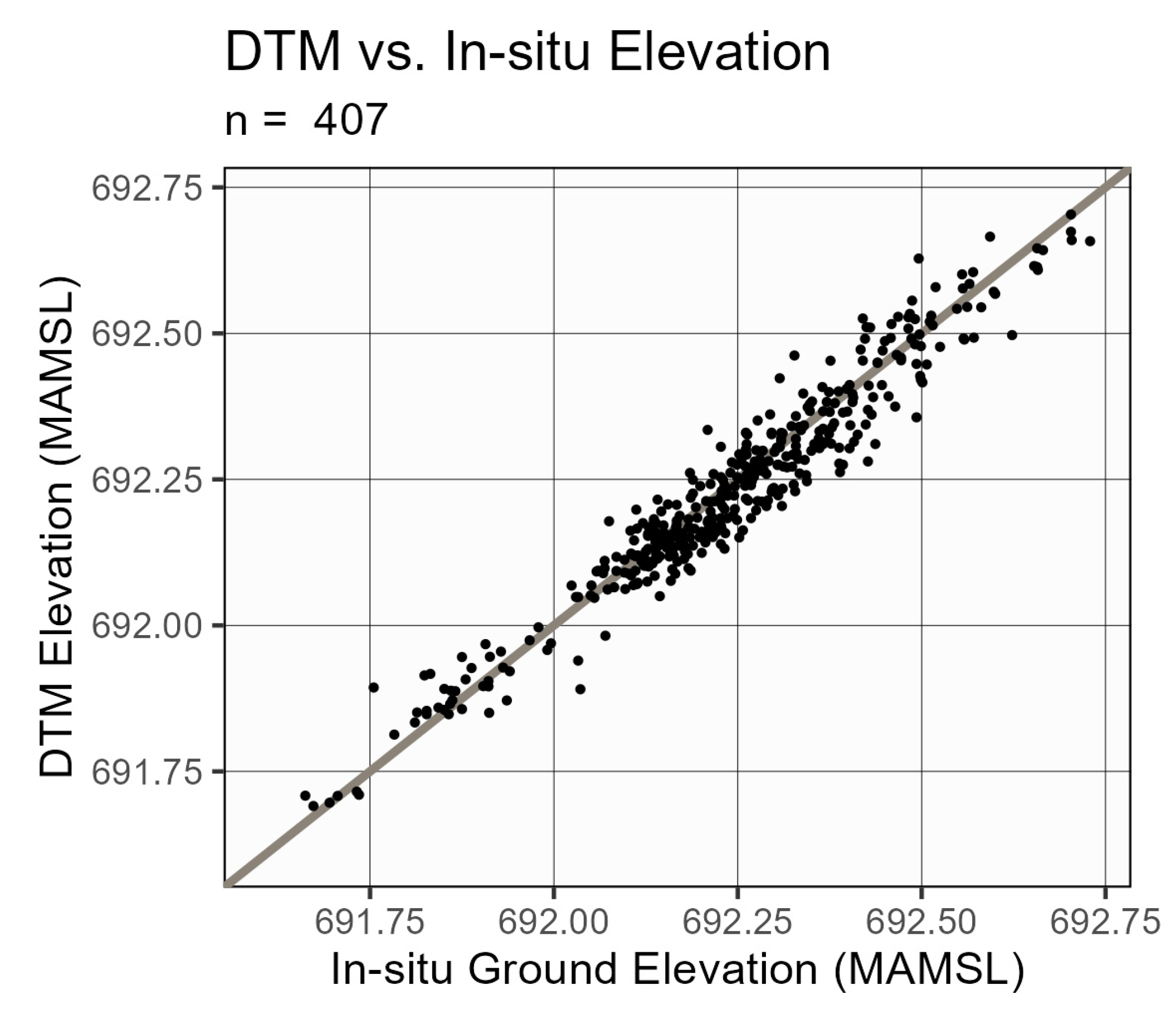
The DTM and water table raster are two important RPAS-derived datasets used in this study (see main text 2 Materials and Methods for how they are created). The DTM is used to quantify elevation deviation and microforms. In addition, it is an input to the depth-to-water (DTW) raster. The water table raster is an intermediate layer used as the other input to create DTW. Therefore, it is imperative that these layers be reasonably accurate.
GNSS surveys of ground elevation and surface water elevation were conducted to provide validation information for the DTM and water table datasets. These surveys occurred within 1 week of the RPAS data collection, with no precipitation events taking place during this period. A systematic sampling scheme was used to collect elevation points along seismic lines. Every 20 m along the seismic lines, the nearest pool of surface water was identified. An elevation measurement was taken at the centre of the pool and in approximately five locations over the nearby ground surface, forming a “cluster” of ground (microtopography) measurements. For the undisturbed matrix, elevation measurements were taken using a random sampling scheme. Forty random spatial points were generated in the matrix and the nearest pool of surface water was identified. Similar to the survey on seismic lines, one elevation measurements was then taken in the centre of the pool and a cluster of five measurements was taken over the nearby ground surface. In total, we surveyed 407 locations of ground elevation and 91 locations of surface water elevation. The survey points were positionally corrected using a post processing kinematic (PPK) workflow.
To validate the DTM, we extracted DTM elevation values at the GNSS-surveyed ground locations. A scatterplot of the DTM vs. GNSS elevation measurements is shown in Figure A1. The brown line is the 1:1 line, and the points fall reasonably along the line. The mean absolute error was 4 cm (Table A1).
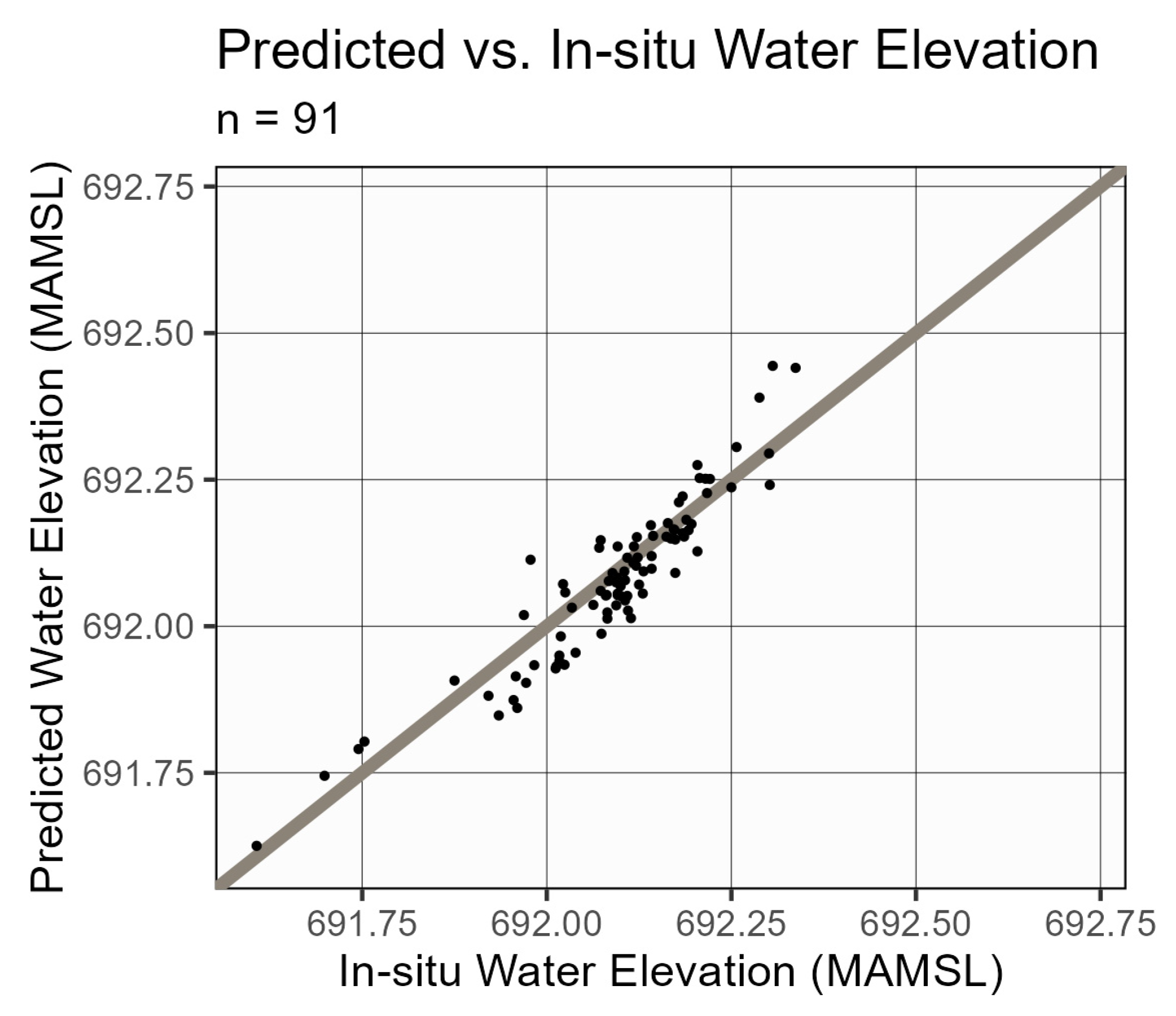
To validate the water table raster, we extracted the interpolated water table elevation values at the GNSS-surveyed surface water locations. A scatterplot of the interpolated water table vs. GNSS elevation measurements is shown in Figure A2. The brown line is the 1:1 line, and the points fall reasonable along the line. The mean absolute error was 4 cm (Table A1).
Figure A1. Scatterplot of ground elevation measurements sourced from GNSS survey and RPAS-derived DTM. The brown line represents the 1:1 line.
Forests 17 00489 g0a1
Figure A2. Scatterplot of surface water elevation measurements sourced from GNSS survey and RPAS-derived interpolated water table raster. The brown line represents the 1:1 line.
Forests 17 00489 g0a2
Table A1. Summary statistics of elevation error between RPAS-derived datasets vs. GNSS-surveyed validation points. Positive values indicate that the GNSS measurement was greater (higher in elevation) than the RPAS measurement. Abbreviations: MAE, mean absolute error; RMSE, root mean square error.
DatasetMin Error (m)Max Error (m)MAE (m)RMSE (m)
Digital terrain model−0.140.150.040.05
Water table raster−0.140.100.040.05

References

  1. Zoltai, S.C.; Vitt, D.H. Canadian Wetlands: Environmental Gradients and Classification. Vegetatio 1995, 118, 131–137. [Google Scholar] [CrossRef]
  2. National Wetlands Working Group. The Canadian Wetland Classification System; Warner, B.G., Rubec, C.D.A., Eds.; Wetlands Research Centre, University of Waterloo: Waterloo, ON, Canada, 1997. [Google Scholar]
  3. Government of Alberta. DRAFT Provincial Woodland Caribou Range Plan; Alberta Ministry of Environment and Parks: Edmonton, AB, Canada, 2017.
  4. Vitt, D.H.; Wieder, R.K.; Scott, K.D.; Faller, S. Decomposition and Peat Accumulation in Rich Fens of Boreal Alberta, Canada. Ecosystems 2009, 12, 360–373. [Google Scholar] [CrossRef]
  5. Government of Alberta. The Alberta Human Footprint Monitoring Program (AHFMP)—A Historical Overview of Geophysical Exploration in Alberta; Alberta Environment and Parks: Edmonton, AB, Canada, 2021.
  6. Dabros, A.; Pyper, M.; Castilla, G. Seismic Lines in the Boreal and Arctic Ecosystems of North America: Environmental Impacts, Challenges, and Opportunities. Environ. Rev. 2018, 26, 214–229. [Google Scholar] [CrossRef]
  7. Timoney, K.; Lee, P. Environmental Management in Resource-Rich Alberta, Canada: First World Jurisdiction, Third World Analogue? J. Environ. Manag. 2001, 63, 387–405. [Google Scholar] [CrossRef]
  8. Shellian, C.A.; Linke, J.; McDermid, G.J.; Cody, M.; Nielsen, S.E. Silviculture Treatments Hasten Seedling Growth on Seismic Disturbances in Boreal Treed Fens. Restor. Ecol. 2024, 32, e14086. [Google Scholar] [CrossRef]
  9. Strack, M.; Hayne, S.; Lovitt, J.; McDermid, G.J.; Rahman, M.M.; Saraswati, S.; Xu, B. Petroleum Exploration Increases Methane Emissions from Northern Peatlands. Nat. Commun. 2019, 10, 2804. [Google Scholar] [CrossRef] [PubMed]
  10. Dyer, S.J.; O’Neill, J.P.; Wasel, S.M.; Boutin, S. Avoidance of Industrial Development by Woodland Caribou. J. Wildl. Manag. 2001, 65, 531–542. [Google Scholar] [CrossRef]
  11. Dyer, S.J.; O’Neill, J.P.; Wasel, S.M.; Boutin, S. Quantifying Barrier Effects of Roads and Seismic Lines on Movements of Female Woodland Caribou in Northeastern Alberta. Can. J. Zool. 2002, 80, 839–845. [Google Scholar] [CrossRef]
  12. Bayne, E.M.; Boutin, S.; Tracz, B.; Charest, K. Functional and Numerical Responses of Ovenbirds (Seiurus aurocapilla) to Changing Seismic Exploration Practices in Alberta’s Boreal Forest. Écoscience 2005, 12, 216–222. [Google Scholar] [CrossRef]
  13. Korsah, P. Effects of Seismic Lines on Peatland Carbon Cycling in Boreal Alberta, Canada. Ph.D. Thesis, University of Waterloo, Waterloo, ON, Canada, 2023. [Google Scholar]
  14. Dickie, M.; McNay, S.R.; Sutherland, G.D.; Cody, M.; Avgar, T. Corridors or Risk? Movement along, and Use of, Linear Features Varies Predictably among Large Mammal Predator and Prey Species. J. Anim. Ecol. 2020, 89, 623–634. [Google Scholar] [CrossRef] [PubMed]
  15. McKenzie, H.W.; Merrill, E.H.; Spiteri, R.J.; Lewis, M.A. How Linear Features Alter Predator Movement and the Functional Response. Interface Focus 2012, 2, 205–216. [Google Scholar] [CrossRef] [PubMed]
  16. Whittington, J.; Hebblewhite, M.; DeCesare, N.J.; Neufeld, L.; Bradley, M.; Wilmshurst, J.; Musiani, M. Caribou Encounters with Wolves Increase near Roads and Trails: A Time-to-Event Approach. J. Appl. Ecol. 2011, 48, 1535–1542. [Google Scholar] [CrossRef]
  17. McDermid, G.J.; Terenteva, I.; Chan, X.Y. Mapping Trails and Tracks in the Boreal Forest Using LiDAR and Convolutional Neural Networks. Remote Sens. 2025, 17, 1539. [Google Scholar] [CrossRef]
  18. Stevenson, C.J.; Filicetti, A.T.; Nielsen, S.E. High Precision Altimeter Demonstrates Simplification and Depression of Microtopography on Seismic Lines in Treed Peatlands. Forests 2019, 10, 295. [Google Scholar] [CrossRef]
  19. Waddington, J.M.; Morris, P.J.; Kettridge, N.; Granath, G.; Thompson, D.K.; Moore, P.A. Hydrological Feedbacks in Northern Peatlands. Ecohydrology 2015, 8, 113–127. [Google Scholar] [CrossRef]
  20. Van Rensen, C.K.; Nielsen, S.E.; White, B.; Vinge, T.; Lieffers, V.J. Natural Regeneration of Forest Vegetation on Legacy Seismic Lines in Boreal Habitats in Alberta’s Oil Sands Region. Biol. Conserv. 2015, 184, 127–135. [Google Scholar] [CrossRef]
  21. Strack, M.; Softa, D.; Bird, M.; Xu, B. Impact of Winter Roads on Boreal Peatland Carbon Exchange. Glob. Change Biol. 2018, 24, e201–e212. [Google Scholar] [CrossRef] [PubMed]
  22. Davidson, S.J.; Goud, E.M.; Franklin, C.; Nielsen, S.E.; Strack, M. Seismic Line Disturbance Alters Soil Physical and Chemical Properties Across Boreal Forest and Peatland Soils. Front. Earth Sci. 2020, 8, 281. [Google Scholar] [CrossRef]
  23. Strack, M.; Mwakanyamale, K.; Hassanpour Fard, G.; Bird, M.; Bérubé, V.; Rochefort, L. Effect of Plant Functional Type on Methane Dynamics in a Restored Minerotrophic Peatland. Plant Soil 2017, 410, 231–246. [Google Scholar] [CrossRef]
  24. Nguyen, P.K.T.; Nam, M.J.; Park, C. A Review on Time-Lapse Seismic Data Processing and Interpretation. Geosci. J. 2015, 19, 375–392. [Google Scholar] [CrossRef]
  25. Coupal, B.; Bentham, P. If You Build It, Will They Come? Caribou Habitat Restoration for Pipeline Projects. In International Pipeline Conference; American Society of Mechanical Engineers: New York, NY, USA, 2014; p. V001T04A009. [Google Scholar] [CrossRef]
  26. Lee, P.; Boutin, S. Persistence and Developmental Transition of Wide Seismic Lines in the Western Boreal Plains of Canada. J. Environ. Manag. 2006, 78, 240–250. [Google Scholar] [CrossRef]
  27. Riva, F.; Acorn, J.H.; Nielsen, S.E. Narrow Anthropogenic Corridors Direct the Movement of a Generalist Boreal Butterfly. Biol. Lett. 2018, 14, 20170770. [Google Scholar] [CrossRef]
  28. Alberta Energy Regulator. Alberta Energy Outlook 2025 (ST98); Alberta Energy Regulator: Calgary, AB, Canada, 2025.
  29. Pinzon, J.; Dabros, A.; Hoffman, P. Soil Mounding as a Restoration Approach of Seismic Lines in Boreal Peatlands: Implications on Microtopography. Restor. Ecol. 2023, 31, e13835. [Google Scholar] [CrossRef]
  30. Rahman, M.M.; McDermid, G.J.; Strack, M.; Lovitt, J. A New Method to Map Groundwater Table in Peatlands Using Unmanned Aerial Vehicles. Remote Sens. 2017, 9, 1057. [Google Scholar] [CrossRef]
  31. Weiland, L.; Green-Harrison, T.; Ketcheson, S. The Influence of Seismic Lines on Wildfire Potential in the Boreal Region of Northern Alberta, Canada. Forests 2023, 14, 1574. [Google Scholar] [CrossRef]
  32. Czapiewski, S.; Szumińska, D. An Overview of Remote Sensing Data Applications in Peatland Research Based on Works from the Period 2010–2021. Land 2022, 11, 24. [Google Scholar] [CrossRef]
  33. Minasny, B.; Adetsu, D.V.; Aitkenhead, M.; Artz, R.R.E.; Baggaley, N.; Barthelmes, A.; Beucher, A.; Caron, J.; Conchedda, G.; Connolly, J.; et al. Mapping and Monitoring Peatland Conditions from Global to Field Scale. Biogeochemistry 2024, 167, 383–425. [Google Scholar] [CrossRef]
  34. Czapiewski, S. Assessment of the Applicability of UAV for the Creation of Digital Surface Model of a Small Peatland. Front. Earth Sci. 2022, 10, 834923. [Google Scholar] [CrossRef]
  35. Isoaho, A.; Ikkala, L.; Marttila, H.; Hjort, J.; Kumpula, T.; Korpelainen, P.; Räsänen, A. Spatial Water Table Level Modelling with Multi-Sensor Unmanned Aerial Vehicle Data in Boreal Aapa Mires. Remote Sens. Appl. Soc. Environ. 2023, 32, 101059. [Google Scholar] [CrossRef]
  36. Lendzioch, T.; Langhammer, J.; Vlček, L.; Minařík, R. Mapping the Groundwater Level and Soil Moisture of a Montane Peat Bog Using UAV Monitoring and Machine Learning. Remote Sens. 2021, 13, 907. [Google Scholar] [CrossRef]
  37. Lovitt, J.; Rahman, M.M.; McDermid, G.J. Assessing the Value of UAV Photogrammetry for Characterizing Terrain in Complex Peatlands. Remote Sens. 2017, 9, 715. [Google Scholar] [CrossRef]
  38. Steenvoorden, J.; Bartholomeus, H.; Limpens, J. Less Is More: Optimizing Vegetation Mapping in Peatlands Using Unmanned Aerial Vehicles (UAVs). Int. J. Appl. Earth Obs. Geoinf. 2023, 117, 103220. [Google Scholar] [CrossRef]
  39. Steenvoorden, J.; Limpens, J. Upscaling Peatland Mapping with Drone-Derived Imagery: Impact of Spatial Resolution and Vegetation Characteristics. GISci. Remote Sens. 2023, 60, 2267851. [Google Scholar] [CrossRef]
  40. Štroner, M.; Urban, R.; Křemen, T.; Braun, J. UAV DTM Acquisition in a Forested Area—Comparison of Low-Cost Photogrammetry (DJI Zenmuse P1) and LiDAR Solutions (DJI Zenmuse L1). Eur. J. Remote Sens. 2023, 56, 2179942. [Google Scholar] [CrossRef]
  41. Natural Regions Committee. Natural Regions and Subregions of Alberta; Downing, D.J.; Pettapiece, W.W. (Compiler) Government of Alberta: Edmonton, AB, Canada, 2006.
  42. Rapidlasso GmbH. LAStools: Efficient LiDAR Processing Software, version 190221; Rapidlasso GmbH: Gilching, Germany, 2019.
  43. Roussel, J.-R.; Auty, D.; Coops, N.C.; Tompalski, P.; Goodbody, T.R.H.; Meador, A.S.; Bourdon, J.-F.; de Boissieu, F.; Achim, A. lidR: An R Package for Analysis of Airborne Laser Scanning (ALS) Data. Remote Sens. Environ. 2020, 251, 112061. [Google Scholar] [CrossRef]
  44. Roussel, J.-R.; Auty, D. lidR: Airborne LiDAR Data Manipulation and Visualization for Forestry Applications, version 4.1.1; Comprehensive R Archive Network (CRAN): Vienna, Australia, 2024.
  45. Pix4Dmapper, version 4.8.0; Pix4D SA: Prilly, Switzerland, 2023.
  46. Therneau, T.; Atkinson, B. Rpart: Recursive Partitioning and Regression Trees, version 4.1.23; Comprehensive R Archive Network (CRAN): Vienna, Australia, 2023.
  47. Gräler, B.; Pebesma, E.; Heuvelink, G. Spatio-Temporal Interpolation Using Gstat. R J. 2016, 8, 204–218. [Google Scholar] [CrossRef]
  48. Pebesma, E.J. Multivariable Geostatistics in S: The Gstat Package. Comput. Geosci. 2004, 30, 683–691. [Google Scholar] [CrossRef]
  49. Queiroz, G.L.; McDermid, G.J.; Rahman, M.M.; Linke, J. The Forest Line Mapper: A Semi-Automated Tool for Mapping Linear Disturbances in Forests. Remote Sens. 2020, 12, 4176. [Google Scholar] [CrossRef]
  50. Lovitt, J.; Rahman, M.M.; Saraswati, S.; McDermid, G.J.; Strack, M.; Xu, B. UAV Remote Sensing Can Reveal the Effects of Low-Impact Seismic Lines on Surface Morphology, Hydrology, and Methane (CH4) Release in a Boreal Treed Bog. J. Geophys. Res. Biogeosci. 2018, 123, 1117–1129. [Google Scholar] [CrossRef]
  51. Golder Associates. Boreal Caribou Habitat Restoration; Golder Associates: Calgary, AB, Canada, 2012. [Google Scholar]
  52. Caners, R.T.; Lieffers, V.J. Divergent Pathways of Successional Recovery for In Situ Oil Sands Exploration Drilling Pads on Wooded Moderate-Rich Fens in Alberta, Canada. Restor. Ecol. 2014, 22, 657–667. [Google Scholar] [CrossRef]
  53. Malhotra, A.; Roulet, N.T.; Wilson, P.; Giroux-Bougard, X.; Harris, L.I. Ecohydrological Feedbacks in Peatlands: An Empirical Test of the Relationship among Vegetation, Microtopography and Water Table. Ecohydrology 2016, 9, 1346–1357. [Google Scholar] [CrossRef]
  54. Kononovs, D.; Rivard, C.; Degenhardt, D.; Snihur, K.N.; Gutierrez-Rueda, D.; Lazowski, C.N.; Rozanitis, K.J.; Coutret, B.; Konhauser, K.O.; Alessi, D.S. Characterizing the Impacts of Seismic Lines on the Water Budget of a Boreal Watershed in Alberta (Western Canada). J. Hydrol. Reg. Stud. 2025, 57, 102133. [Google Scholar] [CrossRef]
  55. Franklin, C.M.A.; Filicetti, A.T.; Nielsen, S.E. Seismic Line Width and Orientation Influence Microclimatic Forest Edge Gradients and Tree Regeneration. For. Ecol. Manag. 2021, 492, 119216. [Google Scholar] [CrossRef]
Figure 1. The study area, a 20-hectare portion of a boreal peatland in northeastern Alberta, Canada. The inset maps provide a more detailed view of (a) the matrix (undisturbed areas) and seismic lines of varying disturbance class, including (b) a new disturbance (created in 2021), (c) an old disturbance (created in 1996), and (d) a re-disturbance (created in 1996, re-cleared in 2021). Seismic line edges are denoted with dotted white lines within the inset maps. Visible water channels in panels (c,d) represent surface water accumulation associated with depressed ground surface conditions.
Forests 17 00489 g001
Figure 2. Example visualizations of the surface morphology and hydrology attributes mapped in this study using RPAS. Abbreviations: MASL, meters above sea level.
Forests 17 00489 g002
Figure 3. Violin plots of elevation deviation (n new disturbance = 70, n old disturbance = 144, n re-disturbance = 53). Elevation deviation is calculated per segment by subtracting the mean elevation of the matrix from the mean elevation of the seismic line. Black dots indicate mean values. Uppercase superscript letters above violins (e.g., A) denote statistical groupings for the mean: groups sharing the same uppercase letter do not differ significantly in mean, whereas groups with different uppercase letters do differ significantly (pairwise Wilcoxon rank-sum tests, BH-adjusted p < 0.05). Abbreviations: Elev, elevation.
Forests 17 00489 g003
Figure 4. (a) Bar plot depicting the proportion of each microform (hummock, lawn and hollow) within segments in the matrix and on seismic lines (n matrix = 267, n new disturbance = 70, n old disturbance = 144, n re-disturbance = 53). (b) Violin plots of hummock proportion deviation (n new disturbance = 70, n old disturbance = 144, n re-disturbance = 53). Hummock proportion deviation is calculated per segment by subtracting the proportion of hummock cover in the matrix from the proportion on the seismic line. Black dots indicate mean values. Uppercase superscript letters above violins (e.g., A, B, C) denote statistical groupings for the mean: groups sharing the same uppercase letter do not differ significantly in mean, whereas groups with different uppercase letters do differ significantly (pairwise Wilcoxon rank-sum tests, BH-adjusted p < 0.05). Abbreviations: Hum_Prop, hummock proportion.
Forests 17 00489 g004
Figure 5. (a) Bar plot depicting the proportion of surface water within segments in the matrix and on seismic lines (n matrix = 267, n new disturbance = 70, n old disturbance = 144, n re-disturbance = 53). (b) Violin plots of surface water proportion deviation (n new disturbance = 70, n old disturbance = 144, n re-disturbance = 53). Surface water proportion deviation is calculated per segment by subtracting the proportion of surface water in the matrix from the proportion on the seismic line. Black dots indicate mean values. Uppercase superscript letters above violins (e.g., A, B) denote statistical groupings for the mean: groups sharing the same uppercase letter do not differ significantly in mean, whereas groups with different uppercase letters do differ significantly (pairwise Wilcoxon rank-sum tests, BH-adjusted p < 0.05). Abbreviations: SW_Prop, surface water proportion.
Forests 17 00489 g005
Figure 6. Violin plots of DTW deviation (n new disturbance = 70, n old disturbance = 144, n re-disturbance = 53). DTW deviation is calculated per segment by subtracting the mean DTW of the matrix from the mean DTW of the seismic line. Black dots indicate mean values. Uppercase superscript letters above violins (e.g., A, B, C) denote statistical groupings for the mean: groups sharing the same uppercase letter do not differ significantly in mean, whereas groups with different uppercase letters do differ significantly (pairwise Wilcoxon rank-sum tests, BH-adjusted p < 0.05). Abbreviations: DTW, depth-to-water.
Forests 17 00489 g006
Figure 7. (a) Conceptual schematic highlighting the major surface morphology and hydrological patterns observed across the three disturbance classes examined in this study. (b) Summary of results from pairwise comparisons of the means and variances of deviation metrics among the three disturbance classes. Blue indicates no statistically significant difference between classes, while yellow indicates a statistically significant difference. For detailed statistical results, see Table 2, Table 3, Table 4 and Table 5.
Forests 17 00489 g007
Table 1. Surface morphology and hydrology metrics under investigation and associated equations, where applicable. Deviation equations are provided where applicable; metrics for which deviation was not calculated are indicated as N/A. Abbreviations: DTW, depth-to-water; Elev, elevation; SW, surface water.
CategoryMetric NameData Product UsedMethod of Aggregation Deviation Equation
Surface
morphology
Elevation
deviation
Digital
terrain model
Mean elevation per segmentMean_ElevLine − Mean_ElevMatrix
Surface
morphology
Hummock
proportion
Microform
raster
Proportion of hummock per segmentN/A
Surface
morphology
Hummock
proportion
deviation
Microform
raster
Proportion of hummock per segmentHummockProportionLine
HummockProportionMatrix
HydrologySW
proportion
SW rasterProportion of water per segmentN/A
HydrologySW
proportion
deviation
SW rasterProportion of water per segmentSW_ProportionLine
SW_ProportionMatrix
HydrologyDTW deviationDTW rasterMean DTW per segmentMean_DTWLine − Mean_DTWMatrix
Table 2. Elevation deviation statistics by disturbance class (n new disturbance = 70, n old disturbance = 144, n re-disturbance = 53). Uppercase superscript letters (e.g., A) denote statistical groupings for the mean: groups sharing the same uppercase letter do not differ significantly in mean, whereas groups with different uppercase letters do differ significantly (pairwise Wilcoxon rank-sum tests, BH-adjusted p < 0.05). Lowercase superscript letters (e.g., a, b) denote statistical groupings for the variance: groups sharing the same lowercase letter do not differ significantly in variance, whereas groups with different lowercase letters do differ significantly (pairwise Brown–Forsythe tests, BH-adjusted p < 0.05).
Disturbance ClassMean (m)Median (m)Min (m)Max (m)SD
(m)
New Disturbance−0.10 A−0.11−0.18−0.040.03 a
Old Disturbance−0.11 A−0.11−0.290.070.07 b
Re-disturbance−0.14 A−0.15−0.31−0.020.06 b
Table 3. Hummock proportion deviation statistics by disturbance class (n new disturbance = 70, n old disturbance = 144, n re-disturbance = 53). Uppercase superscript letters (e.g., A, B, C) denote statistical groupings for the mean: groups sharing the same uppercase letter do not differ significantly in mean, whereas groups with different uppercase letters do differ significantly (pairwise Wilcoxon rank-sum tests, BH-adjusted p < 0.05). Lowercase superscript letters (e.g., a, b, c) denote statistical groupings for the variance: groups sharing the same lowercase letter do not differ significantly in variance, whereas groups with different lowercase letters do differ significantly (pairwise Brown–Forsythe tests, BH-adjusted p < 0.05).
Disturbance ClassMeanMedianMinMaxSD
New Disturbance−0.08 B−0.08−0.220.040.06 a
Old Disturbance−0.05 A−0.06−0.190.230.08 c
Re-disturbance−0.13 C−0.11−0.30−0.020.06 b
Table 4. Surface water proportion deviation by disturbance class (n new disturbance = 70, n old disturbance = 144, n re-disturbance = 53). Uppercase superscript letters (e.g., A, B) denote statistical groupings for the mean: groups sharing the same uppercase letter do not differ significantly in mean, whereas groups with different uppercase letters do differ significantly (pairwise Wilcoxon rank-sum tests, BH-adjusted p < 0.05). Lowercase superscript letters (e.g., a, b) denote statistical groupings for the variance: groups sharing the same lowercase letter do not differ significantly in variance, whereas groups with different lowercase letters do differ significantly (pairwise Brown–Forsythe tests, BH-adjusted p < 0.05).
Disturbance ClassMeanMedianMinMaxSD
New Disturbance0.02 A0.01−0.100.230.07 a
Old Disturbance0.22 B0.16−0.220.840.24 b
Re-disturbance0.24 B0.26−0.100.650.20 b
Table 5. DTW deviation statistics by disturbance class (n new disturbance = 70, n old disturbance = 144, n re-disturbance = 53). Uppercase superscript letters (e.g., A, B, C) denote statistical groupings for the mean: groups sharing the same uppercase letter do not differ significantly in mean, whereas groups with different uppercase letters do differ significantly (pairwise Wilcoxon rank-sum tests, BH-adjusted p < 0.05). Lowercase superscript letters (e.g., a, b, c) denote statistical groupings for the variance: groups sharing the same lowercase letter do not differ significantly in variance, whereas groups with different lowercase letters do differ significantly (pairwise Brown–Forsythe tests, BH-adjusted p < 0.05).
Disturbance ClassMean (m)Median (m)Min (m)Max (m)SD (m)
New Disturbance−0.11 B−0.11−0.19−0.030.03 a
Old Disturbance−0.08 A−0.09−0.270.050.05 c
Re-disturbance−0.13 C−0.13−0.26−0.060.04 b
Disclaimer/Publisher’s Note: The statements, opinions and data contained in all publications are solely those of the individual author(s) and contributor(s) and not of MDPI and/or the editor(s). MDPI and/or the editor(s) disclaim responsibility for any injury to people or property resulting from any ideas, methods, instructions or products referred to in the content.