Abiotic Factors Exert a Predominant Influence on the Annual Aboveground Biomass Dynamics of Chinese Abies Mill. Forests Relative to Biotic Factors

Abstract

The mean annual change in aboveground biomass (ΔAGB) is a pivotal indicator for assessing forest carbon cycle dynamics. This study analyzed 791 independent Abies Mill. forest patches across China to elucidate their driving mechanisms by integrating abiotic, anthropogenic, and biotic factors. We employed a spatially explicit framework, including spatial error regression and structural equation modeling (SEM), to account for significant spatial autocorrelation (Moran’s I = 0.375, p < 0.001). Our results show that abiotic factors predominantly dictate ΔAGB, with soil fertility (pH and Total Nitrogen), elevation (DEM), and soil physical properties (Coarse Fragments and Thickness) explaining the majority of deterministic variance. This relatively low explanatory variance (marginal R² = 0.09) likely reflects the high environmental stochasticity inherent in alpine ecosystems. Specifically, soil fertility exerted the strongest positive influence (Std. Estimate = 0.33), while elevation and soil physical constraints were the primary limiting factors. Biotic factors (Stand Age, Height, and Tree Cover) played a subordinate role, contributing only a marginal 2% gain in explained variance (increasing marginal R² from 0.07 to 0.09). Path analysis revealed an “environmental filtering” hierarchy where abiotic factors shape stand structure, which in turn has limited impact on growth dynamics. These findings underscore that carbon management in alpine forests should prioritize habitat quality conservation over simple biotic structural manipulation.

1. Introduction

The dynamics of Aboveground Biomass (AGB) serve as a key indicator for assessing the carbon sink function of terrestrial ecosystems [1]. In the context of global climate change, understanding the mechanisms driving the mean annual change in forest biomass (ΔAGB) is crucial for predicting regional carbon budgets [2]. Abies Mill. forests, regarded as climax communities in China’s alpine and subalpine zones, play an irreplaceable role in maintaining regional ecological security due to the stability of their carbon pools [3]. These forests not only store a significant amount of biomass carbon but also provide critical ecosystem services, including hydrological regulation, soil conservation, and habitat protection for rare and endangered species.

Ecologists have long debated the relative dominance of biotic factors versus abiotic factors as driving forces behind changes in forest biomass [4]. One perspective posits that biotic factors—such as stand age, canopy height, and tree cover—regulate biomass through niche complementarity or selection effects, both of which are central to carbon sequestration capacity [5,6,7]. Species diversity enhances resource utilization efficiency via functional diversity and niche differentiation, thereby promoting productivity [8]. While this mechanism has been validated across various ecosystems, the influence of biotic factors is often context-dependent [9]. In resource-rich tropical or temperate forests, the positive effects of biodiversity and stand structure are prominent; however, in ecosystems under high environmental stress, these effects may be masked [10,11]. Recent studies suggest that in extreme sub-alpine environments, abiotic constraints may far exceed the intrinsic regulatory capacity of biological communities [12].

In contrast, other studies emphasize that climate (e.g., precipitation and temperature) and soil physicochemical properties (e.g., pH, nutrients, and bulk density) establish the fundamental limits of forest productivity through environmental filtering mechanisms [13,14]. Furthermore, the relationship between biodiversity and productivity is often context-dependent, with environmental filtering becoming the dominant assembly mechanism in harsh climates [9,11]. Soil pH, a critical driver regulating microbial activity and nutrient availability, directly shapes spatial patterns of forest productivity [15]. In nutrient-poor or physically restrictive habitats, edaphic factors often emerge as the primary constraints on growth [12]. Beyond chemical fertility, physical habitat limitations such as soil thickness and coarse fragment content can further restrict root proliferation and biomass accumulation [16]. Particularly in extreme subalpine environments, abiotic constraints may overshadow the regulatory capacity of biological communities [17]. Such ecosystems typically face multiple environmental stresses, such as low temperatures and poor soils; the resulting small species pool leads to community assembly being strongly governed by environmental filtering [10].

Notably, abiotic and biotic drivers do not operate in isolation. Recent studies have demonstrated that climate and soil can indirectly regulate biomass by influencing species diversity and stand structure [13], leading to complex cascading pathways. However, few studies have rigorously quantified the incremental contribution of biotic factors while simultaneously accounting for spatial autocorrelation in these remote alpine regions. This study focuses on the ΔAGB of Abies forests in China. By integrating both abiotic and biotic factors within a spatially explicit framework, we aim to address the following questions: (1) Which abiotic factors (including terrain and soil physical properties) are the core drivers of the spatial variation in ΔAGB? (2) Does the dominance of abiotic factors remain robust under different combinations of biotic factors? By systematically comparing their relative contributions, this study aims to elucidate the regulatory mechanisms of carbon dynamics in Chinese Abies forests, providing a scientific basis for their adaptive management under climate change.

2. Materials and Methods

2.1. Data Collection and Processing

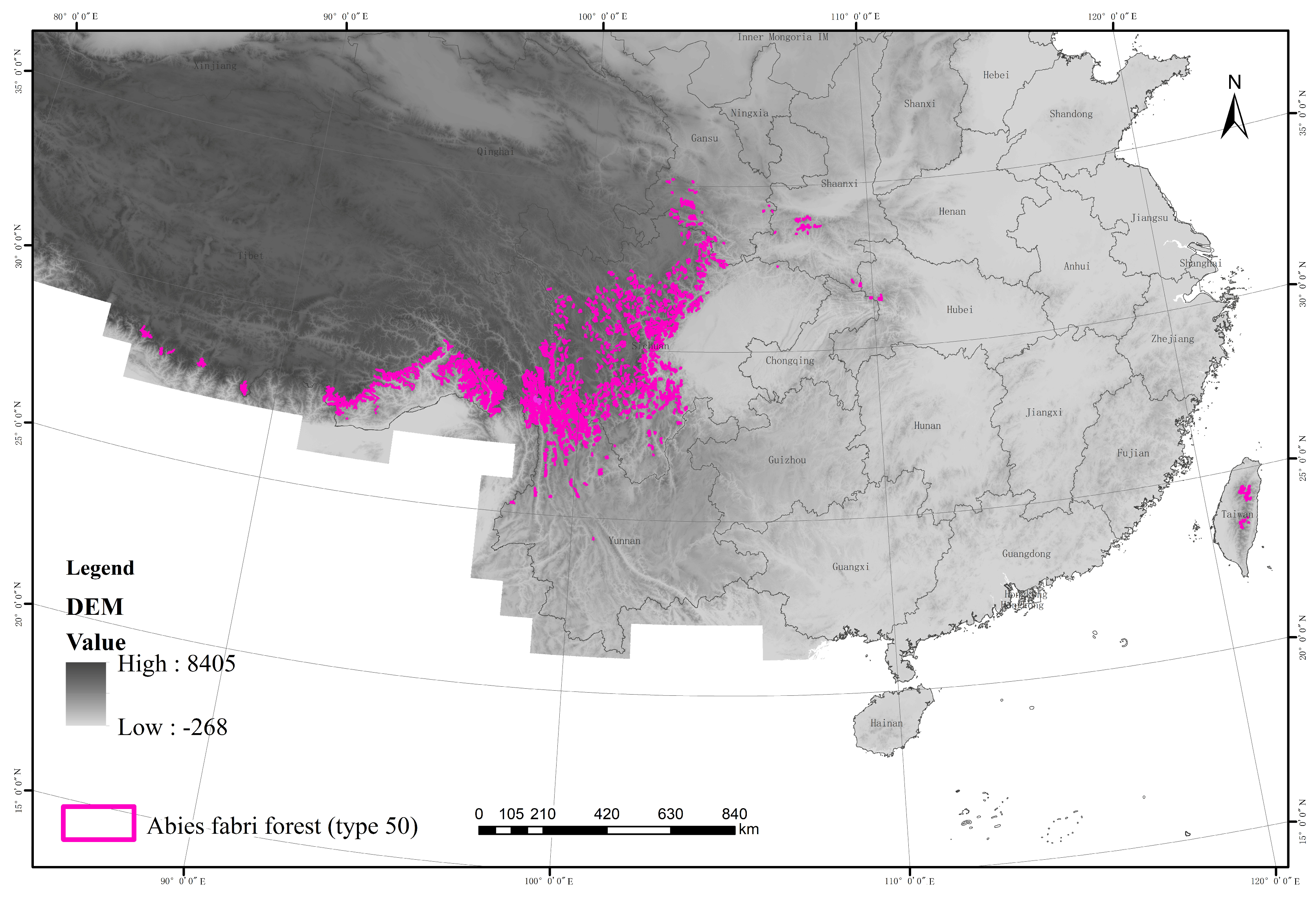
The spatial distribution of Abies forests in China was delineated based on the 1:1,000,000 Vegetation Map of the People’s Republic of China [17]. As illustrated in Figure 1, these forests are predominantly concentrated in the high-altitude mountainous regions of southwestern and central China, areas characterized by complex topography and steep environmental gradients. Although the vegetation map reflects the forest extent as of 2007, Abies forests are recognized as representative climax communities in China’s subalpine zones, characterized by prolonged successional cycles and high structural stability [18]. Such stable community boundaries ensure that the 2007 spatial framework remains highly representative for ecological analysis within our study period, as shifts in the geographic limits of dark coniferous forests are typically multi-decadal processes [19,20]. To ensure high temporal consistency between dependent and independent variables, all dynamic multi-year datasets used in this study—including biomass changes, climate factors, and tree cover—were strictly aligned to the 2013–2020 period. From this synchronized spatial data, a total of 791 independent Abies forest patches were identified and extracted as the primary analytical units [21].

Aboveground Biomass (AGB) Dynamics: Annual AGB products at 30-m resolution were obtained from Yan et al. (2023) via the Science Data Bank (https://www.scidb.cn/en) [21]. Following the method of Holdaway et al. [22], we calculated the mean annual change in AGB (ΔAGB, units: Mg ha⁻¹ yr⁻¹) specifically for the 2013–2020 window. This dynamic indicator serves as the response variable to reflect the recent carbon sequestration rates of Chinese Abies forests.

Abiotic Factors:

Climate Data: Monthly meteorological layers at 1-km resolution, including mean, minimum, and maximum temperatures (TMP, TMN, TMX) and total precipitation (PRE), were retrieved from the Loess Plateau SubCenter of the National Earth System Science Data Center (https://www.geodata.cn). These data were generated using the Delta spatial downscaling scheme [23]. We calculated the multi-year mean values for the 2013–2020 period to represent the stable climate baseline driving biomass changes. Potential evapotranspiration (PET) was integrated using the Hargreaves equation [23].

Soil Data: Daily soil moisture (SM) data at 1-km resolution were sourced from the National Tibetan Plateau Data Center (http://data.tpdc.ac.cn) and averaged over the 2013–2020 period. Additionally, 12 soil physicochemical variables were extracted from the “Chinese soil dataset based on the World Soil Database (HWSD v1.1)” (National Cryosphere Desert Data Center, http://www.ncdc.ac.cn). These data represent harmonized historical profiles primarily collected from the 1980s to the 2000s. Given that fundamental soil properties in alpine ecosystems change slowly over decadal to centennial timescales in the absence of intensive land use change, they serve as a reliable baseline environmental template for constraining forest growth during our study period. These variables are as follows: Soil texture (BD: Soil Bulk Density; CF: Coarse Fragment; CLAY: Clay Fraction; SAND: Sand Fraction; SILT: Silt Fraction; and Thickness) and Soil fertility (CEC: Cation Exchange Capacity; SOC: Organic Carbon; pH: Soil pH; TK: Total Potassium; TN: Total Nitrogen; and TP: Total Phosphorus). Detailed descriptions of these variables are available in previous research [19].

Topographic Data: Topographic features were derived from a 1-km Digital Elevation Model (DEM) obtained from the Resource and Environmental Science Data Platform (https://www.resdc.cn).

Anthropogenic Factor:

Human Footprint (HFP): Anthropogenic pressure was characterized using the annual terrestrial Human Footprint (HFP) index [24]. We utilized the annual HFP layers from 2013 to 2018 (the latest available data overlapping our study period) to calculate a representative average.

Biotic Structure Attributes: Three biotic products initially at 30-m resolution were integrated to quantify stand structural influences, all centered on or averaged within the 2013–2020 window.

Tree Cover (TreeCover): Data were obtained from the CATCD dataset [25]. We averaged the annual layers from 2013 to 2020 to capture the horizontal stand density during the monitoring period.

Stand Height (Height): Arithmetic mean height was retrieved from the national individual tree-based height product [26], representing the peak forest structure (circa 2019–2020) within our study timeframe.

Stand Age (Age): Forest age data for the baseline year 2020 were sourced from the China forest age map [27], providing the successional state at the conclusion of our monitoring window.

All spatial variables were resampled to a consistent 1-km resolution under the GCS_WGS_1984 coordinate system to ensure alignment with the forest patch analytical units.

2.2. Statistical Analysis and Modeling

Prior to modeling, data distributions were evaluated via normality tests, and non-normally distributed variables were log-transformed to satisfy the assumptions of parametric analysis.

To determine the necessity of spatial modeling, we first fitted an initial ordinary least squares (OLS) regression including all 19 abiotic factors and one anthropogenic factor. A Global Moran’s I test was then performed on the OLS residuals to detect spatial dependency. The results confirmed significant positive spatial autocorrelation (Moran’s I = 0.375, p < 0.001), indicating that standard OLS estimates might be biased due to the violation of independence assumptions.

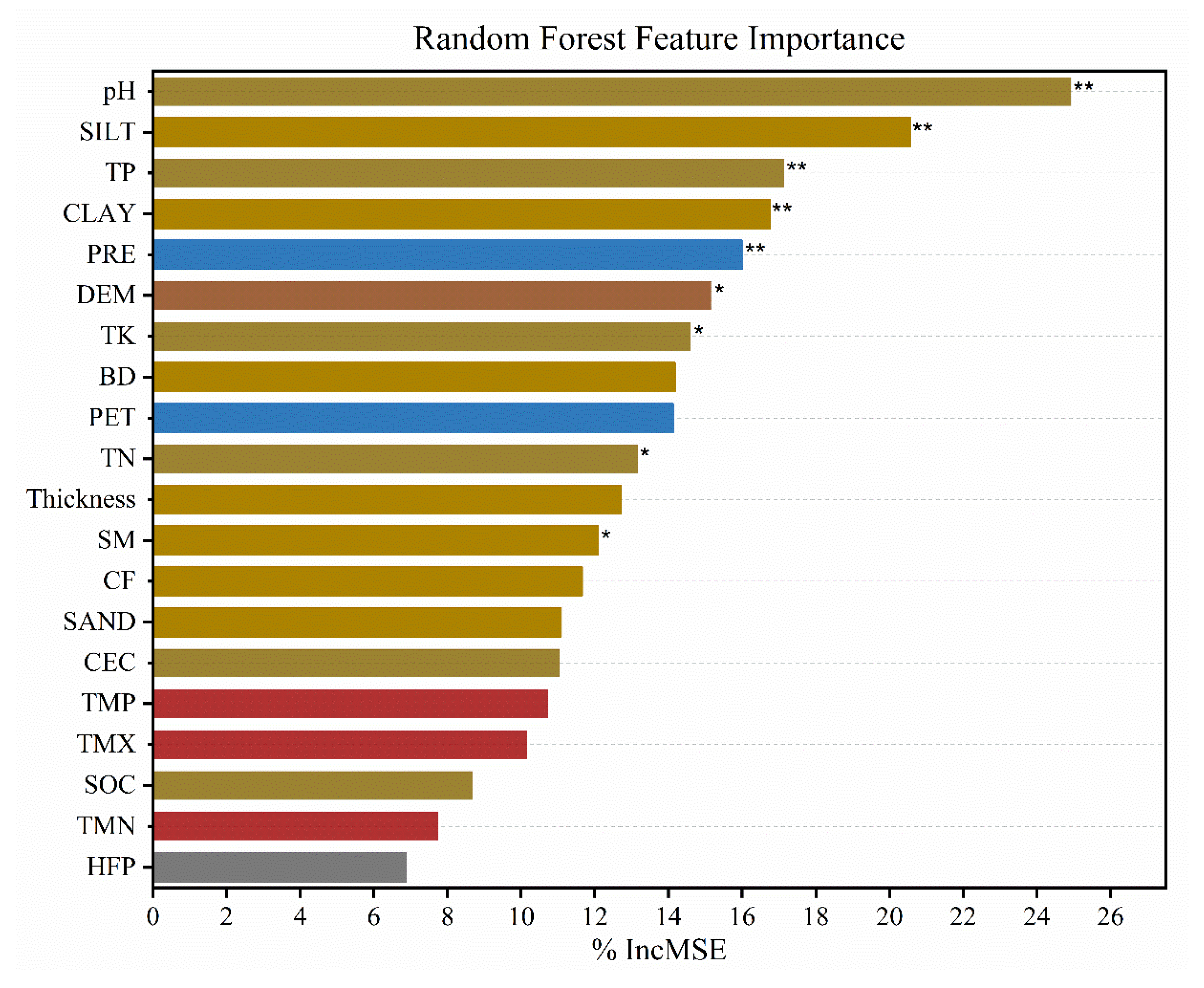
We implemented a robust two-stage variable selection procedure to ensure model parsimony. First, a Random Forest (RF) algorithm was utilized to rank the potential importance of the 20 predictors based on their percentage increase in mean squared error (%IncMSE) for ΔAGB (Figure 2). Second, to formally account for spatial dependency, we transitioned to a Spatial Error Model (SEM/SAR) using the errorsarlm function in the spatialreg R package. Within this spatial framework, we performed backward stepwise elimination; variables were iteratively removed based on the maximum p-value and the minimization of the Akaike Information Criterion (AIC) [28]. This hybrid approach ensured that the selected drivers were both ecologically relevant and statistically robust against spatial autocorrelation.

Based on the principal drivers isolated above, we constructed a piecewise structural equation model (pSEM) using the piecewiseSEM package (version 2.3.0.1) in R (version 4.4.2; R Foundation for Statistical Computing, Vienna, Austria). To maintain consistency with our findings of spatial dependency, each path within the pSEM was modeled using Generalized Least Squares (GLS) from the nlme library (version 3.1.166). We incorporated an exponential correlation structure (corExp) based on the geographic coordinates (Longitude and Latitude) of the patches to explicitly account for spatial autocorrelation in the model residuals. Fisher’s C statistic was used to evaluate the overall goodness of fit.

Finally, we conducted comparative experiments by sequentially introducing biotic factors (Age, Height, and TreeCover) into the baseline abiotic SEM. This allowed us to: (1) quantify the incremental explanatory variance (R² gain) of biotic attributes relative to the abiotic template; and (2) elucidate the cascading pathways through which abiotic drivers indirectly regulate ΔAGB by filtering forest structure.

3. Results

3.1. Core Abiotic Drivers of ΔAGB

Initial diagnostic tests using Ordinary Least Squares (OLS) regression revealed significant spatial autocorrelation in the model residuals (Moran’s I = 0.375, p < 0.001). To account for this spatial dependency and provide more reliable parameter estimates, we upgraded our analytical framework to a Spatial Error Model. Based on the backward stepwise elimination procedure and the minimization of the Akaike Information Criterion (AIC), the refined model identified five key abiotic drivers: pH, TN, DEM, CF, and Thickness (

Table 1. Result of the Spatial Error Model identifying key abiotic drivers of ΔAGB.

Variable	Estimate	Std. Error	Z-Value	p
(intercept)	−13.721	6.327	−2.169	0.030
pH	3.637	0.785	4.635	<0.001
TN	2.171	0.912	2.381	0.017
DEM	−0.0016	0.0005	−2.873	0.004
CF	−0.172	0.079	−2.184	0.029
Thickness	−0.063	0.025	−2.508	0.012
Lambda (λ)	0.758	0.029	26.428	<0.001

).

The Spatial Error Model demonstrated a substantially better fit than the non-spatial model (AIC decreased from 4889.3 to 4545.4). Standardized coefficients indicate that pH remains the most influential positive driver (Estimate = 3.637, p < 0.001), followed by TN (Estimate = 2.171, p = 0.017). These results underscore that soil fertility remains the primary engine for carbon sequestration in Abies forests.

In contrast, topographic and soil physical constraints were identified as the primary limiting factors for biomass dynamics. DEM showed a significant negative association with ΔAGB (Estimate = −0.0016, p = 0.004), suggesting that the harsher physiological conditions at higher altitudes restrict annual biomass increments. Furthermore, soil physical properties, including CF (Estimate = −0.172, p = 0.029) and Thickness (Estimate = −0.063, p = 0.012), also exerted significant negative impacts. Higher rock content and excessive soil depth (which may be linked to poor drainage in alpine zones) represent a restrictive matrix that suppresses biomass accumulation.

The spatial term Lambda (λ) reached 0.758 (p < 0.001), confirming a strong spatial dependency in the growth dynamics of Abies forests. By explicitly incorporating this spatial error term, the model successfully isolated the net effects of abiotic drivers from the underlying spatial patterns, ensuring the robustness of our conclusions.

3.2. Cascading Effects of Abiotic and Biotic Factors

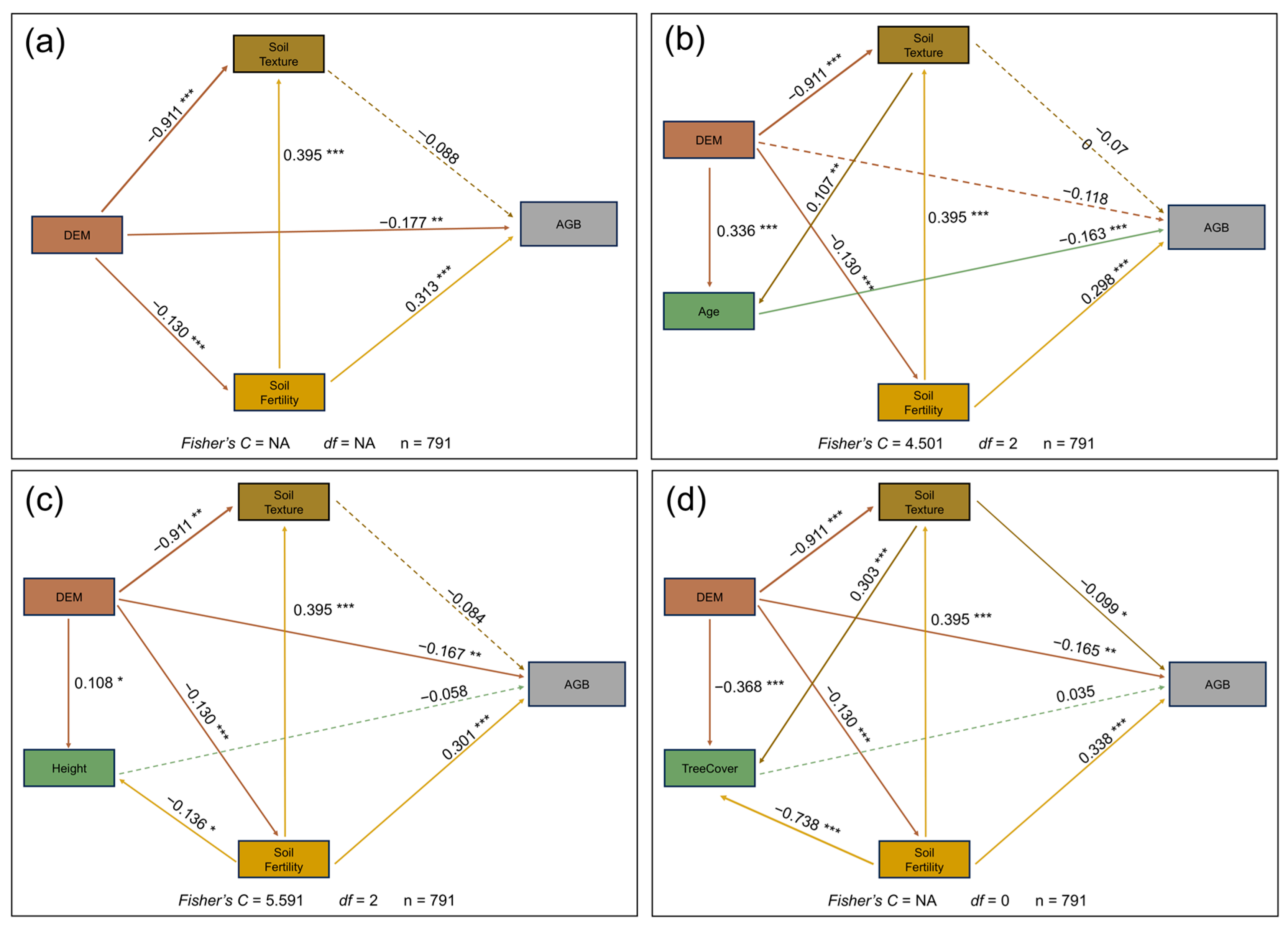
In the baseline model including only abiotic factors (Figure 3a), soil fertility was identified as the most potent direct positive driver of ΔAGB (standardized path coefficient = 0.313, p < 0.001). DEM exhibited a significant direct negative effect (−0.177) and a further indirect negative influence mediated through soil fertility (

Table 2. Standardized total effects of influencing factors on ΔAGB in the structural equation models.

Group	DEM	Soil Texture	Soil Fertility	Age	Height	TreeCover	Explained Variance (R2)
	Total Effect	Total Effect	Total Effect	Total Effect	Total Effect	Total Effect
Only abiotic factors	−0.138	−0.088	0.278	---	—	—	7%
Add different biotic factors	−0.148	−0.087	0.271	−0.163	—	—	7%
	−0.136	−0.084	0.276	—	−0.058	---	7%
	−0.132	−0.089	0.273	—	—	0.035	8%
	−0.147	−0.083	0.269	−0.164	−0.06	—	7%
	−0.142	−0.089	0.266	−0.163	—	0.058	9%
	−0.130	−0.085	0.271	—	−0.057	0.038	8%
	−0.142	−0.085	0.264	−0.164	−0.059	0.062	9%

), likely due to lower nutrient turnover rates in high-altitude regions. The model fit indices (Fisher’s C > 0.05) indicate that the abiotic template—composed of elevation, soil physical properties, and fertility—establishes the fundamental framework for Abies forest growth dynamics. Although the marginal R² remained at a relatively low level, its high stability across various model combinations reflects the potent deterministic constraints imposed by environmental factors on alpine ecosystem productivity.

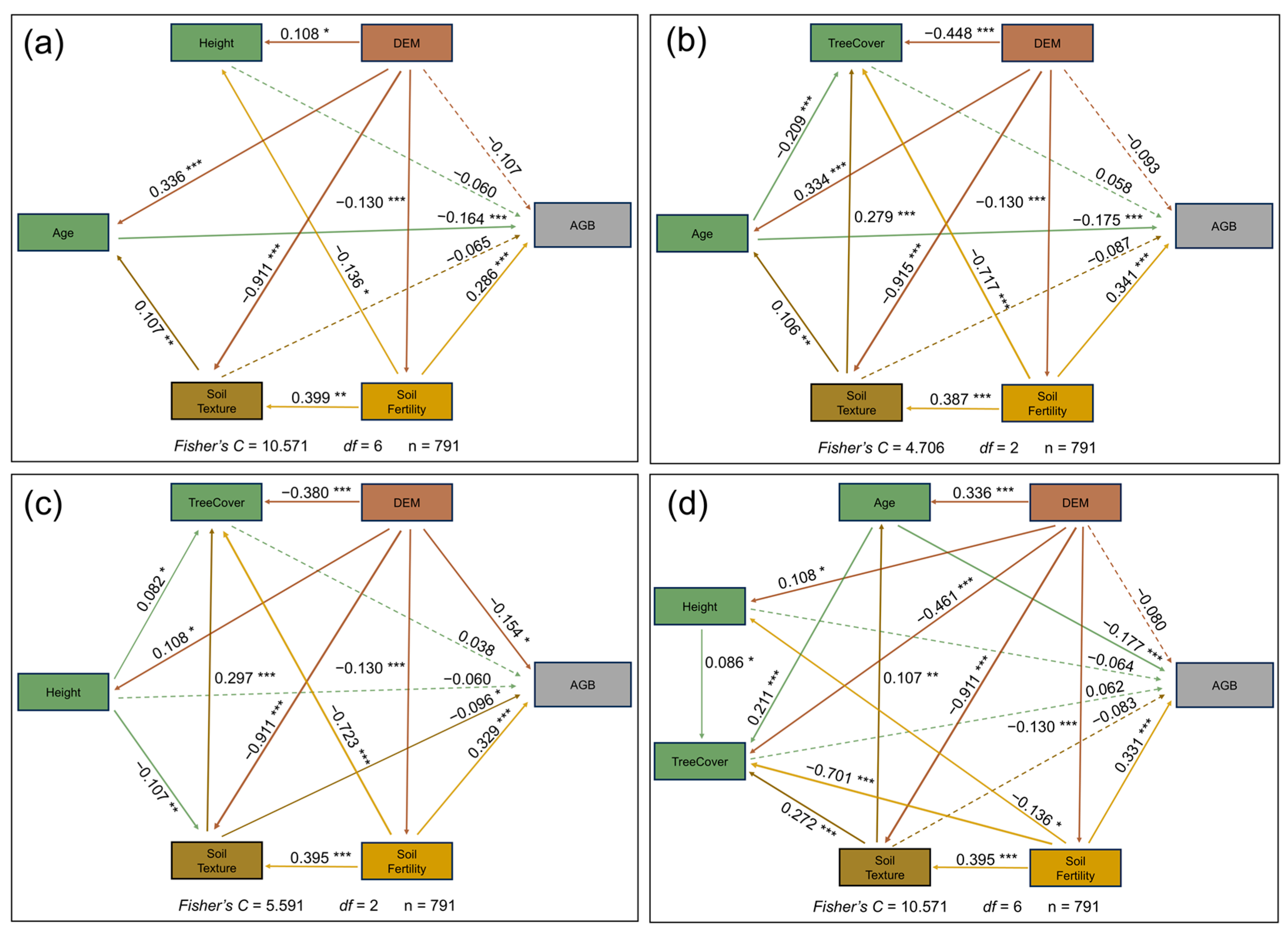
By sequentially and collectively introducing Age, Height, and TreeCover into the baseline model, the marginal contribution of biotic factors to the explained variance (R²) was proven to be extremely limited (Figure 3 and Figure 4). Results indicated that the inclusion of individual biotic factors caused negligible changes in the R² for AGB (remaining between 0.07–0.08). Even in the full model incorporating all three biotic attributes simultaneously (Figure 4d), the R² for AGB only increased from 0.07 to 0.09. This 2% marginal increment provides quantitative evidence that biotic structural variation contributes far less to productivity dynamics than the abiotic environment in these extreme habitats. Furthermore, in the spatially explicit path analysis, the direct impacts of Height and TreeCover on ΔAGB failed to reach statistical significance (p > 0.05). The significant negative direct effect of Age (−0.177) primarily reflects the successional patterns of climax communities, where growth rates naturally decline as stands reach mature or over-mature stages.

Path decomposition analysis (Table 2) further revealed a hierarchical structure of “environmental filtering.” DEM serves as the primary filter, which not only directly constrains growth but also strongly drives an increase in Age (0.336) and a reduction in TreeCover (−0.461). The total effect of soil fertility on ΔAGB (0.264) was substantially higher than the total effect of any biotic factor (e.g., −0.164 for Age and −0.059 for Height). Notably, while abiotic factors exhibited high explanatory variance for structural attributes such as TreeCover (R² reaching 0.46–0.56), these environment-shaped biotic indicators showed weak feedback effects on ΔAGB. This phenomenon points to a significant “biotic decoupling” mechanism in alpine Abies forests, where productivity dynamics are predominantly “locked” by extreme environmental pressures, and the traditional logic of “biotic structure driving growth” is largely overshadowed by environmental filtering.

4. Discussion

4.1. Dominant Role of Abiotic Factors in Carbon Dynamics

This study demonstrates that the mean annual change in aboveground biomass (ΔAGB) of Chinese Abies forests is primarily regulated by an abiotic template consisting of soil chemistry, topography, and soil physical properties. After accounting for significant spatial autocorrelation (λ = 0.758, p < 0.001), which was a critical concern raised during the methodology review, the abiotic factors remained the most potent predictors. The refined model significantly improved the goodness of fit (AIC decreased from 4889.3 to 4545.4), providing a more reliable basis for understanding carbon sequestration in these vulnerable ecosystems compared to non-spatial OLS models.

Among the chemical drivers, pH and TN emerged as the most influential positive drivers. The strong positive impact of pH (β = 3.637) underscores the nutrient-limited nature of alpine forests. In acidic sub-alpine soils, optimal pH levels are essential for catalyzed mineralization and the solubility of limited nutrients, which directly accelerates the growth rate of Abies stands [14,15]. The importance of TN further corroborates that nitrogen availability is a “hard constraint” in high-altitude habitats where low temperatures typically suppress microbial decomposition and nitrogen turnover [12].

DEM exhibited a robust negative influence on ΔAGB, confirming that higher altitudes impose severe physiological limitations through reduced temperatures and shorter growing seasons. Furthermore, the negative impact of CF reflects physical habitat restrictions: high rock content reduces the soil’s water-holding capacity and limits root proliferation, thereby suppressing biomass accumulation. Interestingly, Thickness also showed a negative association, which may suggest that in extreme sub-alpine zones, excessively deep soils are often associated with poor drainage or “meadowization,” which can hinder the productivity of climax coniferous species compared to well-drained, moderate-depth slope soils.

Although the marginal R² of our model (0.07–0.09) might appear low, it is within the expected range for macro-scale studies exploring biomass dynamics (annual change) rather than static stocks. Unlike standing biomass, ΔAGB is highly sensitive to short-term climatic fluctuations and stochastic disturbances typical of alpine environments [29]. The consistency of this R² value across multiple model versions (with and without biotic factors) indicates that the identified abiotic drivers represent the robust, deterministic “ceiling” of forest growth in these regions. These findings support the academic perspective that local habitat heterogeneity, especially edaphic and topographic templates, dictates the productivity of alpine forests more fundamentally than regional climate averages or biotic interactions [30]. Despite these insights, the relatively large proportion of unexplained variance remains a limitation of this study. While the identified abiotic drivers represent the deterministic ‘ceiling,’ the remaining variation may be influenced by fine-scale habitat features that are not fully captured at a 1-km resolution. Future research integrating higher-resolution data, such as UAV-LiDAR or micro-topographic variables (e.g., specific slope positions or aspect-induced moisture differences), would be instrumental in better resolving the impact of fine-scale environmental heterogeneity on these complex alpine forest dynamics.

4.2. Mechanisms Behind the Marginal Contribution of Biotic Factors

Intriguingly, the inclusion of multiple biotic attributes—Age, Height, and TreeCover—yielded a minimal gain in the explained variance of ΔAGB. It is important to note that while other structural metrics, such as mean stand diameter or basal area, are fundamental indicators of forest stand condition, they were not included in this study because spatially continuous, high-resolution (30 m or 1 km) datasets for these variables across the entire national extent of China do not currently exist. Consequently, we utilized stand age, mean canopy height, and tree cover as proxies for the primary vertical and horizontal structural dimensions available at this scale. Our multi-model comparison (Figure 3 and Figure 4) reveals that even in the most complex “Grand Biotic SEM,” the combined incremental R² was only 2% (from 0.07 to 0.09). This quantitative result provides definitive evidence that biotic stand structure plays a subordinate role in driving annual biomass dynamics in Chinese Abies forests.

This phenomenon can be explained by the “environmental filtering” mechanism predominant in high-altitude, cold-climate niches [10,26]. In these stress-prone habitats, abiotic stressors such as low temperatures, nutrient deficiency, and short growing seasons become the primary “hard constraints” on growth [16]. Under such intense environmental pressure, the niche complementarity effects—whereby diverse stand structures or heights enhance resource utilization—are often overshadowed by the necessity for physiological survival [27]. Recent studies have highlighted that in extreme sub-alpine ecosystems, abiotic filters establish a deterministic “ceiling” for productivity that biotic interactions cannot significantly alter [12].

Furthermore, our pSEM results reveal a clear hierarchical structure of control: abiotic factors act as the primary filters that shape stand attributes, which in turn have limited feedback on biomass increments. For instance, DEM and soil fertility exhibited high explanatory variance for Treecover (R² = 0.47) and Soil Texture (R² = 0.56), yet these environment-shaped biotic structures showed non-significant direct effects on ΔAGB (p > 0.05). This suggests a “biotic decoupling” in climax Abies communities, where stand structure primarily reflects the cumulative history of environmental adaptation rather than the current year’s growth potential [9].

It is worth noting that, over centennial to millennial timescales, forest structure can influence soil properties through pedogenic processes. However, our study focuses on an 8-year window of annual biomass change (ΔAGB). On this short ecological timescale, soil physicochemical properties (e.g., pH, TN) act as a relatively stable environmental template rather than being rapidly modified by current stand structure. Furthermore, unlike standard multiple regression which may be biased by multicollinearity, our piecewise SEM explicitly partitions the causal relationship between soil and structure (e.g., Soil Fertility → TreeCover). This structural approach allows us to separate the indirect effects of soil (mediated by structure) from the direct, unique contribution of biotic factors to ΔAGB. Therefore, the potential multicollinearity between soil and structural attributes does not undermine our conclusion that biotic factors provide only marginal unique explanatory variance for ΔAGB (R² gain of 2%).

The significant negative total effect of Age (−0.164) also warrants consideration. This does not represent a positive driver of growth but rather the natural successional decline as climax stands reach maturity [15]. As trees age, their physiological activity and net carbon sequestration rates naturally diminish, particularly in nutrient-limited environments where metabolic turnover is slow. Consequently, the inherent collinearity between environment and structure—where fertile sites support robust stands and nutrient-poor sites result in stunted ones—further diminishes the unique explanatory variance of biotic attributes in our spatial model [14]. This confirms that the direct impact of edaphic and topographic properties on biomass dynamics is significantly more potent than the indirect influence of stand structural variation in these alpine systems.

4.3. Cascading Effects and Management Implications

The spatial SEM pathways underscore a distinct “hierarchy of environmental filtering” driving the biomass dynamics of Abies forests. Our results highlight DEM as the primary upstream filter, which exerts its influence through multiple cascading pathways (Figure 4d). Beyond its direct metabolic constraints, DEM indirectly regulates ΔAGB by modulating soil fertility and stand structural attributes (e.g., Treecover and Age). Specifically, the cascading effect of elevation on soil nutrient turnover reflects the temperature-dependent nature of biogeochemical cycles in alpine regions [28]. By promoting chemical weathering and stimulating microbial activity at lower elevations, the environment enhances the bioavailability of essential elements like Nitrogen, which then acts as the most potent positive driver of carbon sequestration.

These results underscore critical pathways for the sustainable management of Abies ecoregions, particularly under the threat of climate change. Foremost, the finding that biotic stand structures provide only a 2% marginal gain in explanatory variance necessitates a paradigm shift in forest conservation. Traditional “coverage-oriented” approaches, which focus primarily on increasing tree density or afforestation area, may be ineffective in these stress-prone alpine habitats if the underlying edaphic constraints are ignored. Instead, management strategies must transition toward a “habitat-quality-oriented” framework.

Specifically, edaphic integrity must be the cornerstone of carbon management. Given the high sensitivity of Abies growth to soil pH and Nitrogen availability, preventing soil acidification and nutrient depletion is vital for maintaining the physiological baseline of these climax communities. Furthermore, the negative impact of soil physical constraints (Coarse Fragments and Thickness) suggests that soil protection should include preventing compaction and erosion, which are increasingly common due to intensifying extreme precipitation events. Finally, the exclusion of the anthropogenic factor (HFP) from our final predictive model suggests that while these high-altitude forests are currently buffered by their remote locations, their future stability depends more on systemic abiotic changes (e.g., nitrogen deposition and warming-induced soil shifts) than on direct local disturbances. Therefore, long-term monitoring should prioritize altitude-sensitive soil-climate thresholds to ensure the stability of these irreplaceable alpine carbon sinks.

5. Conclusions

This study provides robust, spatially explicit evidence that the annual aboveground biomass dynamics (ΔAGB) in Chinese Abies forests are primarily governed by an abiotic template rather than biotic stand attributes. By employing a rigorous framework of Spatial Error Models (SEMs) and piecewise SEMs with GLS, we effectively accounted for significant spatial autocorrelation, ensuring the reliability of our parameter estimates. Our findings reveal a distinct “hierarchy of environmental filtering,” where abiotic factors—specifically elevation (DEM), soil fertility (pH and TN), and soil physical constraints (Coarse Fragments and Thickness)—establish the fundamental limits of carbon sequestration in these high-altitude ecosystems.

Among the identified drivers, soil fertility emerged as the most potent positive engine of growth, while elevation and soil physical properties constituted the core constraints. Most notably, the inclusion of key biotic structural attributes (stand age, mean height, and tree cover) provided only a marginal 2% gain in explained variance (R² from 0.07 to 0.09), and vertical structural attributes (height and cover) failed to show significant direct effects. This quantitative evidence identifies a “biotic decoupling” phenomenon in stress-prone alpine habitats, where potent environmental filtering overshadows the niche complementarity effects typically observed in resource-rich forests.

Despite these robust findings, this study has certain limitations. Due to the challenges of data acquisition at a national scale across remote alpine patches, our model did not incorporate species diversity or functional trait variables. These biotic components can influence biomass dynamics through niche complementarity; however, previous research in high-stress environments [11] suggests that abiotic filters typically override the effects of biological diversity. This supports our observation of relatively low marginal R² values, indicating that annual growth variation is primarily constrained by a deterministic abiotic “ceiling” rather than biotic interactions.

In light of these results, we emphasize a necessary paradigm shift in forest conservation and carbon management. Future strategies in alpine regions should transition from a traditional “coverage-oriented” approach to a comprehensive “habitat-quality-oriented” strategy. Prioritizing edaphic integrity—specifically by preventing soil acidification, compaction, and nutrient depletion—is essential to ensure the long-term stability and carbon sink capacity of these irreplaceable alpine climax communities in a changing global climate.

References

1. Pan, Y.; Birdsey, R.A.; Fang, J.; Houghton, R.; Kauppi, P.E.; Kurz, W.A.; Phillips, O.L.; Shvidenko, A.; Lewis, S.L.; Canadell, J.G.; et al. A Large and Persistent Carbon Sink in the World’s Forests. Science 2011, 333, 988–993. [Google Scholar] [CrossRef]
2. Chave, J.; Réjou-Méchain, M.; Búrquez, A.; Chidumayo, E.; Colgan, M.S.; Delitti, W.B.C.; Duque, A.; Eid, T.; Fearnside, P.M.; Goodman, R.C.; et al. Improved Allometric Models to Estimate the Aboveground Biomass of Tropical Trees. Glob. Change Biol. 2014, 20, 3177–3190. [Google Scholar] [CrossRef] [PubMed]
3. Dakhil, M.A.; Xiong, Q.; Farahat, E.A.; Zhang, L.; Pan, K.; Pandey, B.; Olatunji, O.A.; Tariq, A.; Wu, X.; Zhang, A.; et al. Past and Future Climatic Indicators for Distribution Patterns and Conservation Planning of Temperate Coniferous Forests in Southwestern China. Ecol. Indic. 2019, 107, 105559. [Google Scholar] [CrossRef]
4. Chen, R.; Ran, J.; Hu, W.; Dong, L.; Ji, M.; Jia, X.; Lu, J.; Gong, H.; Aqeel, M.; Yao, S.; et al. Effects of Biotic and Abiotic Factors on Forest Biomass Fractions. Natl. Sci. Rev. 2021, 8, nwab025. [Google Scholar] [CrossRef]
5. Liang, J.; Crowther, T.W.; Picard, N.; Wiser, S.; Zhou, M.; Alberti, G.; Schulze, E.-D.; McGuire, A.D.; Bozzato, F.; Pretzsch, H.; et al. Positive Biodiversity-Productivity Relationship Predominant in Global Forests. Science 2016, 354, aaf8957. [Google Scholar] [CrossRef] [PubMed]
6. Poorter, L.; van der Sande, M.T.; Thompson, J.; Arets, E.J.M.M.; Alarcón, A. Diversity Enhances Carbon Storage in Tropical Forests. Glob. Ecol. Biogeogr. 2015, 24, 1314–1328. [Google Scholar] [CrossRef]
7. Sullivan, M.J.P.; Talbot, J.; Lewis, S.L.; Phillips, O.L.; Qie, L.; Begne, S.K.; Chave, J.; Cuni-Sanchez, A.; Hubau, W.; Lopez-Gonzalez, G.; et al. Diversity and Carbon Storage across the Tropical Forest Biome. Sci. Rep. 2017, 7, 39102. [Google Scholar] [CrossRef]
8. Facelli, J.M. The Functional Consequences of Biodiversity. Empirical Progress and Theoretical Extensions. Austral Ecol. 2003, 28, 684–685. [Google Scholar] [CrossRef]
9. Kohyama, T.I.; Sheil, D.; Sun, I.-F.; Niiyama, K.; Suzuki, E.; Hiura, T.; Nishimura, N.; Hoshizaki, K.; Wu, S.-H.; Chao, W.-C.; et al. Contribution of Tree Community Structure to Forest Productivity across a Thermal Gradient in Eastern Asia. Nat. Commun. 2023, 14, 1113. [Google Scholar] [CrossRef]
10. Kaushal, S.; Baishya, R. Stand Structure and Species Diversity Regulate Biomass Carbon Stock under Major Central Himalayan Forest Types of India. Ecol. Process. 2021, 10, 14. [Google Scholar] [CrossRef]
11. Homeier, J.; Leuschner, C. Factors Controlling the Productivity of Tropical Andean Forests: Climate and Soil Are More Important than Tree Diversity. Biogeosciences 2021, 18, 1525–1541. [Google Scholar] [CrossRef]
12. Li, F.; Shi, Z.; Liu, S.; Chen, M.; Xu, G.; Chen, J.; Xing, H. Stand Structural Diversity and Edaphic Properties Regulate Aboveground Biomass of Abies Fargesii Var. Faxoniana Primary Forest on the Eastern Qinghai-Tibetan Plateau. Eur. J. For. Res. 2024, 143, 1401–1410. [Google Scholar] [CrossRef]
13. Ali, A.; Lin, S.-L.; He, J.-K.; Kong, F.-M.; Yu, J.-H.; Jiang, H.-S. Climate and Soils Determine Aboveground Biomass Indirectly via Species Diversity and Stand Structural Complexity in Tropical Forests. For. Ecol. Manag. 2019, 432, 823–831. [Google Scholar] [CrossRef]
14. Quesada, C.A.; Lloyd, J.; Schwarz, M.; Patiño, S.; Baker, T.R.; Czimczik, C.; Fyllas, N.M.; Martinelli, L.; Nardoto, G.B.; Schmerler, J.; et al. Variations in Chemical and Physical Properties of Amazon Forest Soils in Relation to Their Genesis. Biogeosciences 2010, 7, 1515–1541. [Google Scholar] [CrossRef]
15. Wu, W.; Liu, H.-B. Estimation of Soil pH with Geochemical Indices in Forest Soils. PLoS ONE 2019, 14, e0223764. [Google Scholar] [CrossRef] [PubMed]
16. Whalley, W.R.; Bengough, A.G.; Hawkesford, M.J.; Mooney, S.J.; Bennett, M.J.; Pandey, B.K. Soil Mechanical Resistance and Root Growth and Function. In Plant Roots: The Hidden Half, 5th ed.; CRC Press: Boca Raton, FL, USA, 2024. [Google Scholar]
17. Moser, G.; Leuschner, C.; Hertel, D.; Graefe, S.; Soethe, N.; Iost, S. Elevation Effects on the Carbon Budget of Tropical Mountain Forests (S Ecuador): The Role of the Belowground Compartment. Glob. Change Biol. 2011, 17, 2211–2226. [Google Scholar] [CrossRef]
18. Fang, J.; Wang, Z.; Tang, Z. Atlas of Woody Plants in China: Distribution and Ecology; Springer: Berlin/Heidelberg, Germany, 2011. [Google Scholar]
19. Xiang, X.; Gao, M.; Zhou, Z. Fossil History and Modern Distribution of the Genus Abies (Pinaceae). Front. For. China 2007, 2, 355–365. [Google Scholar] [CrossRef]
20. Mobaied, S.; Machon, N.; Lalanne, A.; Riera, B. The Spatiotemporal Dynamics of Forest–Heathland Communities over 60 Years in Fontainebleau, France. IJGI 2015, 4, 957–973. [Google Scholar] [CrossRef]
21. Yan, S.; He, G.; Zhang, X. Forest Aboveground Biomass Products in China, 2013–2021. Sci. Data Bank 2023, 118, 103275. [Google Scholar]
22. Holdaway, R.J.; Easdale, T.A.; Carswell, F.E.; Richardson, S.J.; Peltzer, D.A.; Mason, N.W.H.; Brandon, A.M.; Coomes, D.A. Nationally Representative Plot Network Reveals Contrasting Drivers of Net Biomass Change in Secondary and Old-Growth Forests. Ecosystems 2017, 20, 944–959. [Google Scholar] [CrossRef]
23. Peng, S.; Ding, Y.; Wen, Z.; Chen, Y.; Cao, Y.; Ren, J. Spatiotemporal Change and Trend Analysis of Potential Evapotranspiration over the Loess Plateau of China during 2011–2100. Agric. For. Meteorol. 2017, 233, 183–194. [Google Scholar] [CrossRef]
24. Mu, H.; Li, X.; Wen, Y.; Huang, J.; Du, P.; Su, W.; Miao, S.; Geng, M. A Global Record of Annual Terrestrial Human Footprint Dataset from 2000 to 2018. Sci. Data 2022, 9, 176. [Google Scholar] [CrossRef]
25. Cai, T.; Xu, X.; Zhu, P.; Nie, S.; Wang, C.; Xiong, Y.; Liu, X. Unveiling Spatiotemporaltree Cover Patterns in China: The First 30 m Annual Tree Cover Mapping from 1985 to 2023. ISPRS J. Photogramm. Remote Sens. 2024, 216, 240–258. [Google Scholar] [CrossRef]
26. Chen, Y.; Yang, H.; Yang, Z.; Yang, Q.; Liu, W.; Huang, G.; Ren, Y.; Cheng, K.; Xiang, T.; Chen, M.; et al. Enhancing High-Resolution Forest Stand Mean Height Mapping in China through an Individual Tree-Based Approach with Close-Range Lidar Data. Earth Syst. Sci. Data 2024, 16, 5267–5285. [Google Scholar] [CrossRef]
27. Cheng, K.; Chen, Y.; Xiang, T.; Yang, H.; Liu, W.; Ren, Y.; Guan, H.; Hu, T.; Ma, Q.; Guo, Q. A 2020 Forest Age Map for China with 30 m Resolution. Earth Syst. Sci. Data 2024, 16, 803–819. [Google Scholar] [CrossRef]
28. Dormann, C.F.; McPherson, J.M.; Araújo, M.B.; Bivand, R.; Bolliger, J.; Carl, G. Methods to Account for Spatial Autocorrelation in the Analysis of Species Distributional Data: A Review. Ecography 2007, 30, 609–628. [Google Scholar] [CrossRef]
29. Qin, X.; Sun, J.; Wang, X. Plant Coverage Is More Sensitive than Species Diversity in Indicating the Dynamics of the Above-Ground Biomass along a Precipitation Gradient on the Tibetan Plateau. Ecol. Indic. 2018, 84, 507–514. [Google Scholar] [CrossRef]
30. Van Der Sande, M.T.; Peña-Claros, M.; Ascarrunz, N.; Arets, E.J.M.M.; Licona, J.C.; Toledo, M.; Poorter, L. Abiotic and Biotic Drivers of Biomass Change in a Neotropical Forest. J. Ecol. 2017, 105, 1223–1234. [Google Scholar] [CrossRef]
Figure 1. Spatial distribution of the 791 independent Abies Mill. forest patches analyzed in this study across China.
Forests 17 00466 g001
Figure 2. Result of the random forest. Variable importance measured as the percent increase in mean squared error (% IncMSE) when the variable is permuted. Higher values indicate greater influence on model prediction. Bar colors indicate different groups of predictors. Asterisks indicate significance levels (* p < 0.05; ** p < 0.01). Abbreviations: pH, soil pH; SILT, silt fraction; TP, total phosphorus; CLAY, clay fraction; PRE, annual precipitation; DEM, elevation; TK, total potassium; BD, soil bulk density; PET, potential evapotranspiration; TN, total nitrogen; Thickness, soil thickness; SM, soil moisture; CF, coarse fragments; SAND, sand fraction; CEC, cation exchange capacity; TMP, mean annual temperature; TMX, annual maximum temperature; SOC, soil organic carbon; TMN, annual minimum temperature; HFP, human footprint index.
Forests 17 00466 g002
Figure 3. Graphical results of the structural equation models. Variables are represented by individual variable names for single-component factors and categorical names for composite factors. Solid single arrows indicate significant paths, while dashed single arrows represent non-significant paths. The values associated with the single arrows denote the standardized path coefficients. Asterisks indicate significance levels (* p < 0.05; ** p < 0.01; *** p < 0.001). (a) SEM considering only abiotic factors; (b) SEM model with biotic factor Age added; (c) SEM model with biotic factor Height added; (d) SEM model with biotic factor TreeCover added.
Forests 17 00466 g003
Figure 4. Graphical results of the structural equation model. Meanings of arrows and symbols are as in Figure 3. Asterisks indicate significance levels (* p < 0.05; ** p < 0.01; *** p < 0.001). (a) SEM incorporating biotic factors Age and Height; (b) SEM incorporating biotic factors Age and TreeCover; (c) SEM incorporating biotic factors Height and TreeCover; (d) SEM incorporating biotic factors Age, Height and TreeCover.
Forests 17 00466 g004