Remote Sensing Aboveground Biomass Inversion of Four Vegetation Types in the Nanji Wetland

Abstract

Aboveground biomass (AGB) serves as a crucial indicator for assessing vegetation carbon sequestration capacity. While AGB levels vary significantly across different vegetation types and regions, the spatial distribution of AGB for specific wetland communities remains poorly characterized. To address this, we integrated field-collected data with Sentinel-2 spectral bands and remote sensing indices, employing random forest (RF) regression and Backpropagation Neural Network (BPNN) for AGB modeling. Through comparative evaluation of their inversion performance, the optimal model was selected to estimate vegetation AGB in the Nanji Wetland. By incorporating wetland classification data, we further generated spatial distribution maps of AGB for four dominant vegetation types during the dry season. The main findings are as follows. Important variables for the RF model included spectral bands B12, B11, B3, B2, B9, B1, B8, B6, and B4 and the Modified Normalized Difference Water Index (MNDWI), Normalized Difference Water Index (NDWI), Kernel Normalized Difference Vegetation Index (KNDVI), and Simple Ratio Index (SR). RF demonstrated significantly higher predictive accuracy (R² = 0.945, RMSE = 109.205 g·m⁻²) compared to the BPNN (R² = 0.821, RMSE = 176.025 g·m⁻²). The total estimated AGB reached 4.03 × 10⁹ g; Carex spp. dominated AGB accumulation (1.49 × 10⁹ g), followed by P. australis spp. (6.69 × 10⁸ g), M. lutarioriparius spp. (4.60 × 10⁸ g), and Polygonum spp. (3.61 × 10⁸ g). The AGB exhibited a clear spatial gradient, decreasing from higher-elevation lakeshore areas towards the central lake. The results provide detailed spatial quantification of AGB stocks across dominant vegetation types, revealing distinct spatial characteristics and interspecies variations in AGB. This study offers a valuable baseline and methodological framework for monitoring wetland carbon dynamics.

1. Introduction

Aboveground biomass (AGB) serves as a critical metric for evaluating wetland ecological functions and plays a vital role in assessing the carbon sequestration potential of wetland vegetation [1,2]. Global studies indicate substantial carbon stocks in various wetland ecosystems. For instance, seasonally dry tropical forests can store 8.7 Pg C in AGB with a potential capacity of 22.1 Pg [3]. Similarly, mangroves exhibit an average AGB carbon storage of 78.0 ± 64.5 tC·ha⁻¹ and a sequestration rate of 2.9 ± 2.2 tC·ha⁻¹·yr⁻¹ [4]. At regional scales, the Bohai Rim coastal wetlands of China can hold 211 Tg C in AGB [5], while the Songnen Plain has an average AGB carbon density of 111.01 g·C·m⁻², increasing substantially at 2.04 g·C·m⁻²·yr⁻¹ [6]. Freshwater wetlands also contribute notably to carbon storage. For example, Kolonnawa Wetland and Thalawathugoda Wetland Park in Sri Lanka showed AGB carbon stocks ranging from 13.79 ± 3.65 to 66.49 ± 6.70 tC·ha⁻¹ and 8.13 ± 2.42 to 52.63 ± 10.00 tC·ha⁻¹, respectively [1]. Given these findings, accurate AGB estimation is essential for quantifying regional carbon sequestration dynamics.

The AGB of different regions and vegetation types exhibits notable spatial variation due to influences from natural geography and climatic factors. From a natural geographical perspective, Zhou [7] demonstrated that coastal wetlands exhibit higher AGB (3.1 kg·m⁻²) compared to that of inland wetlands (1.47 kg·m⁻²). On the Qinghai–Tibet Plateau, the average AGB reached 100.78 g·m⁻² in 2020, with distinct spatial patterns showing lower values in the northwest and higher values in the southeastern grasslands, indicating a clear northwest-to-southeast increasing gradient [8]. Similarly, Zang [9] employed remote sensing to estimate dry grassland biomass in Northeast China, finding that most grassland areas had biomass levels <300 g·m⁻². Further differentiation of wetland types enhances estimation accuracy, as reported by Jin [10], where distinguishing between saltwater and freshwater marshes markedly improves AGB assessment for reed communities. Additionally, Jensen [11] observed that the AGB peaks of herbaceous species in the lower intertidal zone decline with increasing elevation and show a slight resurgence at higher altitudes.

Climatic factors, particularly precipitation and temperature, play crucial roles in AGB dynamics. Sun [5] developed a vegetation index-based AGB inversion model for the Bohai Sea coastal wetlands, incorporating remote sensing, topographic, and climatic data. Their findings revealed that precipitation enhances AGB growth by increasing soil moisture and reducing salinity. Wang [6] confirmed the notable influence of precipitation by demonstrating that increased summer and autumn rainfall promotes vegetation growth and consequently boosts AGB, while maximum temperatures show a strong positive correlation with AGB. In the Sanjiang Plain, Liu [12] documented a notable AGB density increase of 2.47 g·C·m⁻²·yr⁻¹, averaging ~282.05 g·C·m⁻², with winter precipitation negatively impacting AGB and July temperatures positively affecting it. Ren [13] documented a notable AGB density increase of 2.47 g·C·m⁻²·yr⁻¹, averaging ~282.05 g·C·m⁻², with winter precipitation negatively impacting AGB and July temperatures positively affecting it. The deep neural network analysis of forest AGB by Lv [14] in the Tumen River Basin revealed temperature-dependent precipitation effects—below −2 °C, AGB accumulation shows minimal response to precipitation, while above this threshold, increased precipitation correlates with slight AGB reduction. Beyond natural environmental factors, AGB distribution is also influenced by hydrological processes [15] and exhibits strong correlations with anthropogenic activities at local scales [16].

Remote sensing offers important advantages for AGB estimation, including broad spatial coverage, rapid data acquisition, and high efficiency. Consequently, remote sensing-based AGB estimation has attracted considerable scholarly attention, yielding extensive research. Conventional parametric regression methods have been used in AGB reversion [17,18]. However, studies have proved that ecological relationships often exhibit non-linearity; hence, many scholars adopted non-linear regression models when conducting remote sensing inversion [19]. For instance, Li [20] leveraged Sentinel-2 spectral and texture features with random forest (RF) and Extreme Gradient Boosting (XGBoost) algorithms to estimate grassland AGB in Shengjin Lake, Anhui Province. Wan [21] mapped AGB based on RF and Landsat Images. Li [22] compared six machine learning algorithms and found that the RF algorithm had the best effect in estimating the aboveground biomass of grasslands. Lyu [23] found that the inversion effect of the BPNN was better than that of the multi-factor parameter model and the single-factor parameter model. Since both RF and the BPNN demonstrate good inversion performance, we selected these two methods and compared their performance for AGB inversion in Nanji Wetland.

A review of the existing research reveals that the current research on AGB inversion has the following problems. Remote sensing-based inversion of multi-species vegetation biomass remains relatively underexplored. Most studies on wetland vegetation biomass inversion have predominantly focused on single-species estimation, particularly targeting dominant or invasive species such as Spartina alterniflora [16,24], Zizania latifolia [25], Carex spp. [17,25], Cyperus papyrus [26], and P. australis [27,28,29]. To date, only Wan [21] has investigated four typical lake wetland plants (Carex cinerascens, Phalaris arundinacea, Artemisia, and Miscanthus sacchariflorus), while Wu [30] has conducted inversion studies on Scirpus spp., Spartina alterniflora, and Phragmites australis. These studies confirmed substantial variations in AGB across different plant types [31]. The Nanji Wetland, as a representative of the lake wetlands in the middle and lower reaches of the Yangtze River, features a complex landscape of seasonally submerged sandbars, water bodies, and grass islands and serves as an important carbon pool. In complex wetland ecosystems, like Poyang Lake, where multiple vegetation types exhibit alternating distribution patterns, relying solely on a single dominant species for total biomass estimation can lead to notable inaccuracies [32].

Another problem is that the spatial heterogeneity of AGB distribution among different vegetation types was not addressed. For wetland vegetation, biomass dynamics are strongly influenced by hydrological fluctuations [28,33], particularly in environments like the Nanji Wetland of Poyang Lake, where pronounced environmental gradients [34] result in distinct annular or arc-shaped vegetation distributions along water-level and elevation gradients [35,36]. While pooled modeling across vegetation types mitigates sample size limitations and simplifies field sampling, species-specific modeling provides more accurate biomass estimates for individual wetland vegetation types [30]. However, few studies have successfully characterized the spatial distribution patterns of AGB in multi-species wetland vegetation under constrained sample conditions. As for remote sensing inversion, the water level gradient often reflects the overall situation of the region and is difficult to reflect spatial heterogeneity. Hence, most remote sensing inversion studies employ vegetation indices or bands as primary predictors [17,37], with some incorporating plant height data [10].

Research on wetland biomass inversion is conducive to accurately estimating the carbon sequestration capacity of wetland vegetation. By combining wetland classification and AGB inversion, this study aims to establish an inversion model applicable to the AGB of the Nanji Wetland and reveal the distribution characteristics of AGB across its four vegetation types to provide a framework for wetland carbon estimation.

2. Data and Methodology

2.1. Study Area

The study area is on the southwestern shore of Poyang Lake (116°10′–116°25′ E, 28°51′–29°08′ N) at the delta front formed by the confluence of the north, middle, and south branches of the Ganjiang River. It is bordered by Poyang, Yugan, Nanchang, and Duchang counties to the east, south, west, and north, respectively, spanning 21.6 km (east–west) and 27.7 km (north–south). Centred on the Nanji Wetland National Nature Reserve, Jiangxi Province, the study encompasses a 15 km radius from its geographic centroid (hereinafter “Nanji Wetland”; Figure 1). The area (804.85 km² in total; 329.31 km² within the reserve) comprises 26 saucer-shaped lakes, excluding non-wetland zones (settlements, farmlands, and forests).

The Nanji Wetland hosts 443 vascular plant species (304 genera, 115 families), with six dominant families: Polygonaceae, Rosaceae, Fabaceae, Asteraceae, Poaceae, and Cyperaceae. The floristic composition is primarily tropical–subtropical–temperate, with cosmopolitan families also present. Herbaceous species (71% of total flora) dominate, notably aquatic, hygrophytic, and palustrine taxa [38]. Key species include Phragmites australis (P. australis), Miscanthus lutarioriparius (M. lutarioriparius), Carex spp., and Phalaris arundinacea. P. australis and M. lutarioriparius communities occur near the lakeshore (16–18 m elevation with P. australis at slightly higher elevations), while Carex spp. dominate shoals further inland (14–16 m). Phalaris arundinacea thrives near central water bodies (13 m elevation) [35,36]. As a critical stopover on the East Asia–Australasia flyway, the wetlands support 45 waterbird species (12 families, 7 orders), with annual populations ranging from 11,000 to 33,000 individuals [39].

2.2. Data Sources

2.2.1. Sampling Points and Collection of AGB

In accordance with the requirement of no less than three sample plots for each type of vegetation, we collected a total of 133 different vegetation samples from the lakeshore to the lake center from October to November 2023. The central point of each quadrat was georeferenced using an RTK Differential Global Positioning System device, and surface cover conditions were documented (Figure 1). Aboveground vegetation was harvested using the mowing method and dried in an oven at 65 °C for 48 h until reaching a constant weight. The dry biomass (g·m⁻²) was recorded. Surface soil samples (0–20 cm depth) were collected using the five-point sampling method. After thorough mixing, the composite samples were placed in self-sealing bags. Following grinding, soil organic carbon (SOC) content was determined using the potassium dichromate volumetric method. Soil samples for moisture determination were collected using 100 cm³ core cutters. Soil moisture was measured using the oven-drying method.

A total of 133 vegetation samples were collected, encompassing dominant species such as M. lutarioriparius, Carex spp., P. australis, Juncus effusus (J. effusus), Zizania latifolia (Z. latifolia), Polygonum criopolitanum (P. criopolitanum), Persicaria orientalis (P. orientalis), and Persicaria lapathifolium (P. lapathifolium). Notably, Carex spp. emerged as a keystone species in the study area, frequently occurring in mixed stands with P. australis, P. lapathifolium, M. lutarioriparius, J. effusus, and Z. latifolia, exhibiting a distinct stratified growth pattern.

2.2.2. Preprocessing of Sentinel-2 Images

To align with the field sampling period, Sentinel-2 L2A satellite imagery from October to November 2023 was selected based on two criteria: (1) acquisition dates between October and November and (2) cloud cover <10%. The data were retrieved from the Copernicus Open Access Hub (https://dataspace.copernicus.eu/ (accessed on 24 May 2024)). For subsequent spectral analysis, all bands were resampled to a uniform 10 m spatial resolution using SNAP (Sentinel Application Platform; https://step.esa.int/main/download/snap-download/ (accessed on 24 May 2024)). Key vegetation and water indices were then derived from the processed imagery (

Table 1. Remote sensing index.

Remote Sensing Index	Calculation Formula
NDVI (Normalized Difference Vegetation Index)	$NDVI={\displaystyle \frac{NIR-R}{NIR+R}}$
kNDVI (Kernel Normalized Difference Vegetation Index)	$kNDVI=tanh\left(NDV{I}^2\right)$ [40]
EVI (Enhanced Vegetation Index)	$EVI=2.5\times {\displaystyle \frac{NIR-R}{NIR+6\times R-7.5\times B+1}}$
SAVI (Soil-Adjusted Vegetation Index)	$SAVI={\displaystyle \frac{(NIR-R)}{(NIR+R+0.5)}}\times (1+0.5)$
NIRv (Near-Infrared Reflectance of Vegetation)	$NIRv=NIR\times {\displaystyle \frac{NIR-R}{NIR+R}}$
NDWI (Normalized Difference Water Index)	$NDWI={\displaystyle \frac{G-NIR}{G+NIR}}$
MNDWI (Modified Normalized Difference Water Index)	$MNDWI={\displaystyle \frac{G-SWIR}{G+SWIR}}$
SR (Simple Ratio Index)	$SR={\displaystyle \frac{NIR}{R}}$

).

2.3. Research Methods

2.3.1. Random Forest

Random forest, proposed by Breiman [41], is an ensemble method that builds multiple decision trees, each trained on an independently sampled random vector. Predictions are made via majority voting, and as the forest grows, the generalization error stabilizes. The model’s performance depends on individual tree strength and inter-tree correlation. RF outperforms linear regression [42,43] due to its noise robustness, computational efficiency, and ability to capture non-linear patterns. It also resists overfitting and handles noisy data effectively, leading to widespread use in biomass estimation [26,37,44,45]. To enhance model generalizability, RF employs random feature selection by reducing the number of parameters to simplify the model and shorten the training time and by enhancing the generalization ability to reduce overfilling and avoid excessive dimensions. The basis of feature optimization is to calculate the importance of feature variables, also known as the mean decrease in accuracy (MDA) of feature variables. The MDA calculation formula is as follows:

$$MDA={\displaystyle \frac{\sum ({Accuracy}_2-{Accuracy}_1)}{N_{tree}}}$$

(1)

where ${Accuracy}_1$ represents the initial accuracy of the model and ${Accuracy}_2$ is the accuracy rate after adding the interference. $N_{tree}$ indicates that there are N decision trees in the random forest.

Using Google Earth Engine, we performed an RF classification based on spectral bands, remote sensing indices, and texture features, with 80% of samples for training and 20% for validation. For the inversion process, feature importance assessment was first conducted to identify significant feature variables with a cumulative contribution rate exceeding 90%. Subsequently, 80% of the samples were used as training data and 20% as validation data for RF regression.

2.3.2. Backpropagation Neural Network

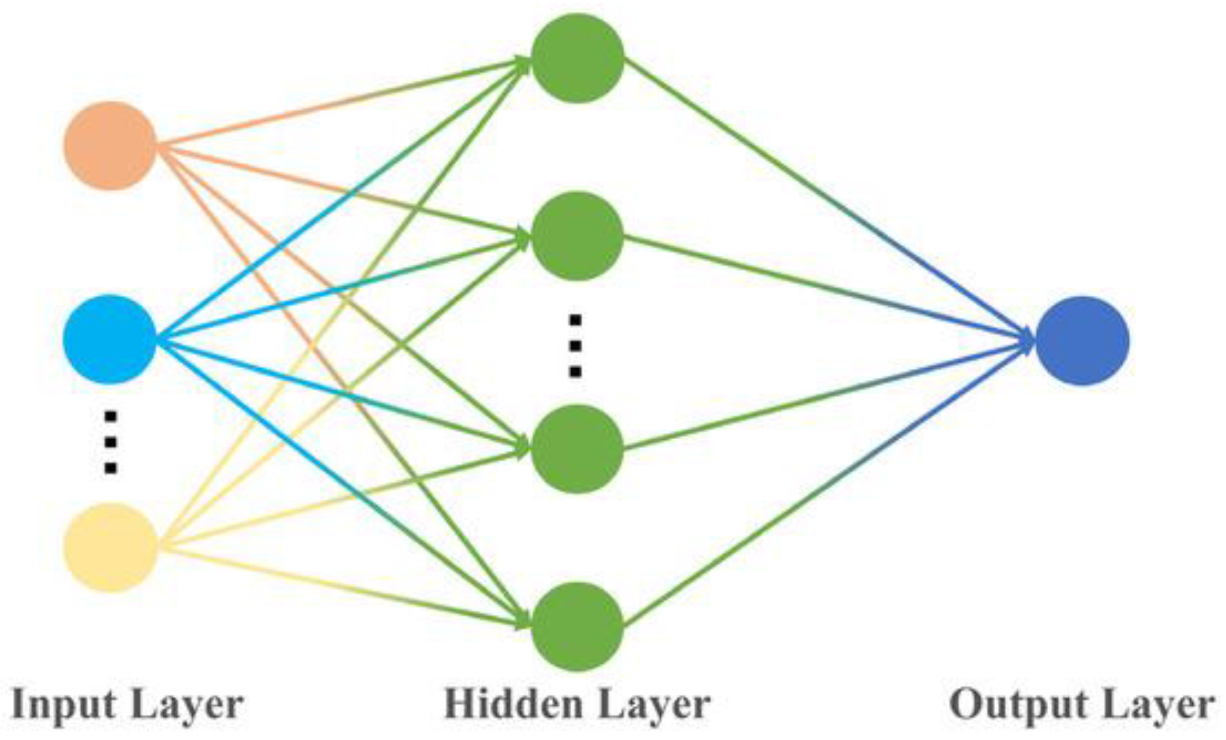
The Backpropagation Neural Network (BPNN) was first proposed by Rumelhart et al. in 1986 [46]. Their seminal paper, “Learning Representations by Back-Propagating Errors,” brought widespread attention to the algorithm. The BPNN is a classic and widely adopted multilayer feedforward artificial neural network. Its core principle lies in utilizing the error backpropagation algorithm for training. The network architecture typically comprises an input layer, at least one hidden layer, and an output layer. The framework of this model is shown in Figure 2. Signals propagate forward layer by layer from the input layer; after processing through weighted summation and non-linear activation functions within the hidden layer neurons, predictions are generated at the output layer. During training, the prediction is compared with the desired target value to obtain the error. The critical step is backpropagation: this error signal propagates backward in the reverse direction of the forward path (layer by layer from the output layer back to the input layer).

2.3.3. Model Accuracy Evaluation

Wetland classification accuracy evaluation. The overall accuracy (OA) and Kappa coefficient are indicators commonly used for evaluating classification accuracy. Here, the OA and Kappa coefficient are calculated based on the confusion matrix to evaluate the wetland classification accuracy. The OA calculation formula is as follows:

$$OA={\displaystyle \frac{{\sum }_{i=1}^n{x}_{ii}}{{\sum }_{i=1}^n{\sum }_{j=1}^n{x}_{ij}}}$$

(2)

where $n$ represents the number of categories,$x_{ii}$ is the number of samples whose actual data belong to the $i$-th category but are classified as the $j$-th category (when $i$ = $j$, it is the number of correctly classified samples, that is $x_{ii}$ represents the number of samples whose actual and classified results both belong to the $i$-th category), and ${\sum }_{j=1}^n{x}_{ij}$ is the total number of samples.

The Kappa calculation formula is as follows:

$$Kappa={\displaystyle \frac{p_o-p_e}{1-p_e}}$$

(3)

where $p_o$ is the total accuracy of the actual classification and $p_e$ is the expected classification accuracy, and the calculation formula of $p_e$ is as follows:

$$p_e={\sum }_{i=1}^n\left({\displaystyle \frac{{\sum }_{j=1}^n{x}_{ij}{\sum }_{k=1}^n{x}_{ki}}{{\left({\sum }_{i=1}^n{\sum }_{j=1}^n{x}_{ij}\right)}^2}}\right)$$

(4)

where $n$ represents the number of categories and $x_{ii}$ has the same calculation formula as described in the previous formula; ${\sum }_{k=1}^n{x}_{ki}$ represents the sum of the elements in the $i$-th column of the confusion matrix (i.e., the total number of samples whose predicted category is $i)$; and ${\sum }_{i=1}^n{\sum }_{j=1}^n{x}_{ij}$ represents the sum of all elements in the confusion matrix (i.e., the total number of samples $n$).

Model accuracy evaluation. Commonly used model accuracy evaluation indicators include R² and the root mean square error (RMSE), and their calculation formulas are as follows:

$$R^2=1-{\displaystyle \frac{{{\sum }_{i=1}^n(y_i-{\widehat{y}}_i)}^2}{{\sum }_{i=1}^n(y_i-{\stackrel{-}{y}}_i)}}$$

(5)

$$RMSE=\sqrt{{\displaystyle \frac{1}{n}}{\sum }_{i=1}^n{\left(y_i-{\widehat{y}}_i\right)}^2}$$

(6)

where $n$ is the number of samples, $y_i$ is the actual value of the $i$-th observation, ${\widehat{y}}_i$ is the predicted value of the $i$-th observation, and ${\stackrel{-}{y}}_i$ is the average value of all observations.

2.3.4. Research Roadmap

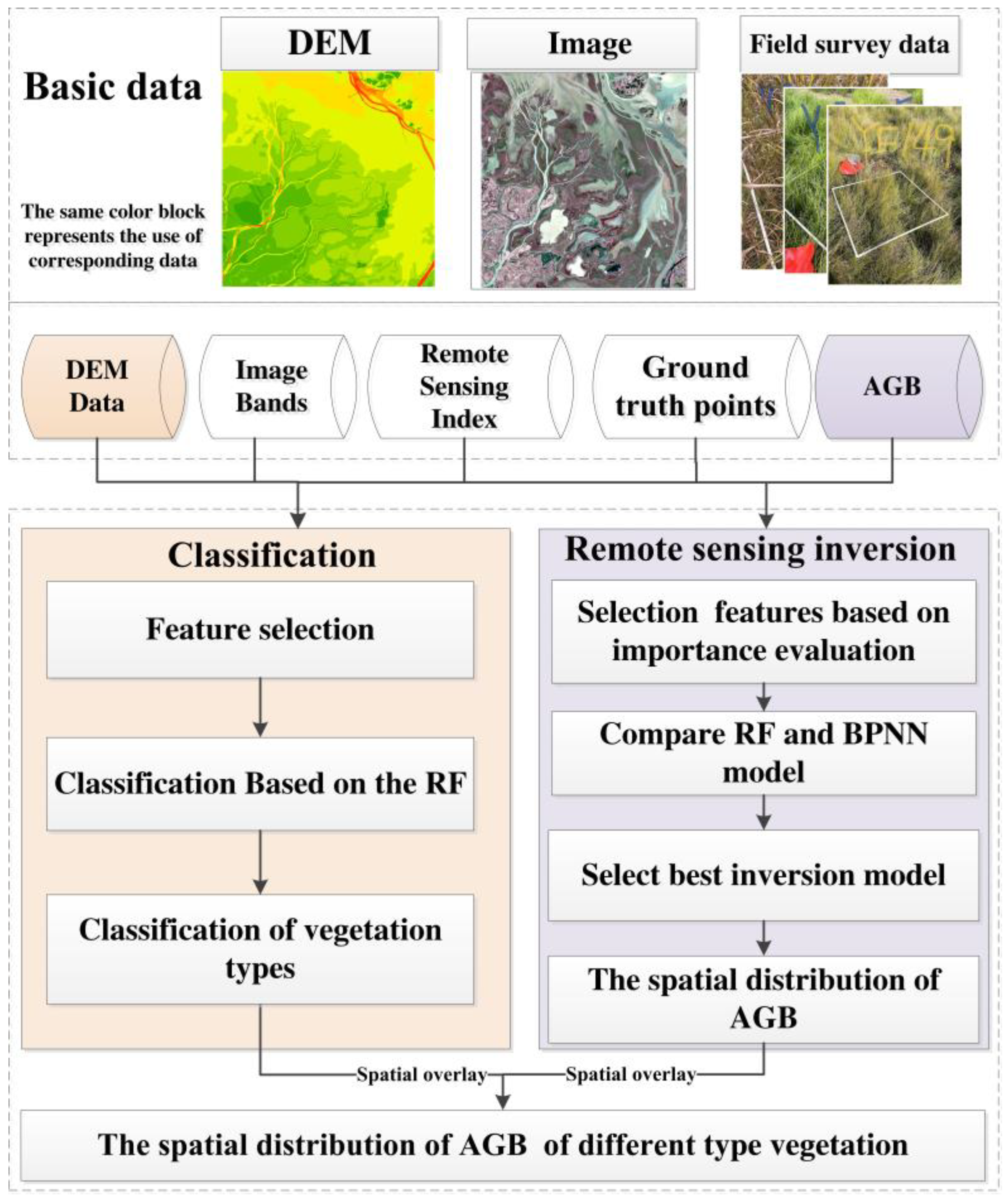
This study characterized AGB patterns across wetland vegetation types by integrating wetland classification results with spatial distribution data through overlay analysis (Figure 3). The classification utilized Sentinel-2 spectral bands, DEM data, ground truth points, and remote sensing indices (Table 1), supplemented by texture features derived from Principal Component Analysis (PCA) and the Gray-Level Co-occurrence Matrix (GLCM). Specifically, PCA was applied to Sentinel-2’s 12 spectral bands in ENVI 5.6 (Harris Geospatial Solutions, Broomfield, CO, USA). to extract the first principal component. GLCM analysis of this component then generated eight texture parameters: mean, variance, homogeneity, contrast, dissimilarity, entropy, second moment, and correlation. For AGB inversion, spectral bands and Table 1 indices served as initial feature variables. We evaluated variable importance, retaining those achieving a cumulative contribution > 90%. Both RF and BPNN models were developed and systematically compared, and the optimal model was selected for AGB retrieval.

3. Results

3.1. Statistical Characteristic Analyses of Vegetation AGB in the Nanji Wetland

The statistical analysis (

Table 2. Vegetation basic conditions.

Vegetation Types	Mean Elevation (m)	Mean AGB (g·m−2)
Carex	12.77	625.32
Carex and J. effusus	13.21	413.33
J. effusus	12.83	197.50
M. lutarioriparius	13.57	1026.67
M. lutarioriparius_ Carex	13.96	914.44
P. australis	13.40	1122.27
P. australis_Carex	13.48	1188.46
P. criopolitanum	11.92	310.00
P. lapathifolium	13.77	868.33
P. lapathifolium_Carex	13.39	603.33
P. orientalis	12.70	1038.33
Z. latifolia	13.49	645.00
Z. latifolia_Carex	12.53	786.67

Note: The 1985 National Elevation Datum is adopted as the elevation datum.

) reveals terrain elevation and AGB characteristics among the studied vegetation communities. Carex spp. predominantly occurs within the 12.77 m elevation, with the M. lutarioriparius_Carex community occupying the highest terrain elevation (13.96 m), followed by P. australis_Carex (13.48 m) and P. lapathifolium_Carex (13.39 m) communities. Notably, the P. australis_Carex community exhibited the highest AGB (1188.46 g·m⁻²), which is over six-fold greater than that of J. effusus (the lowest biomass community). For Carex spp. specifically, our measurements show considerably higher autumn biomass (625.32 g·m⁻²) compared to the winter values (346.85 g·m⁻²) reported by Yu [48], suggesting strong seasonal variation in biomass production.

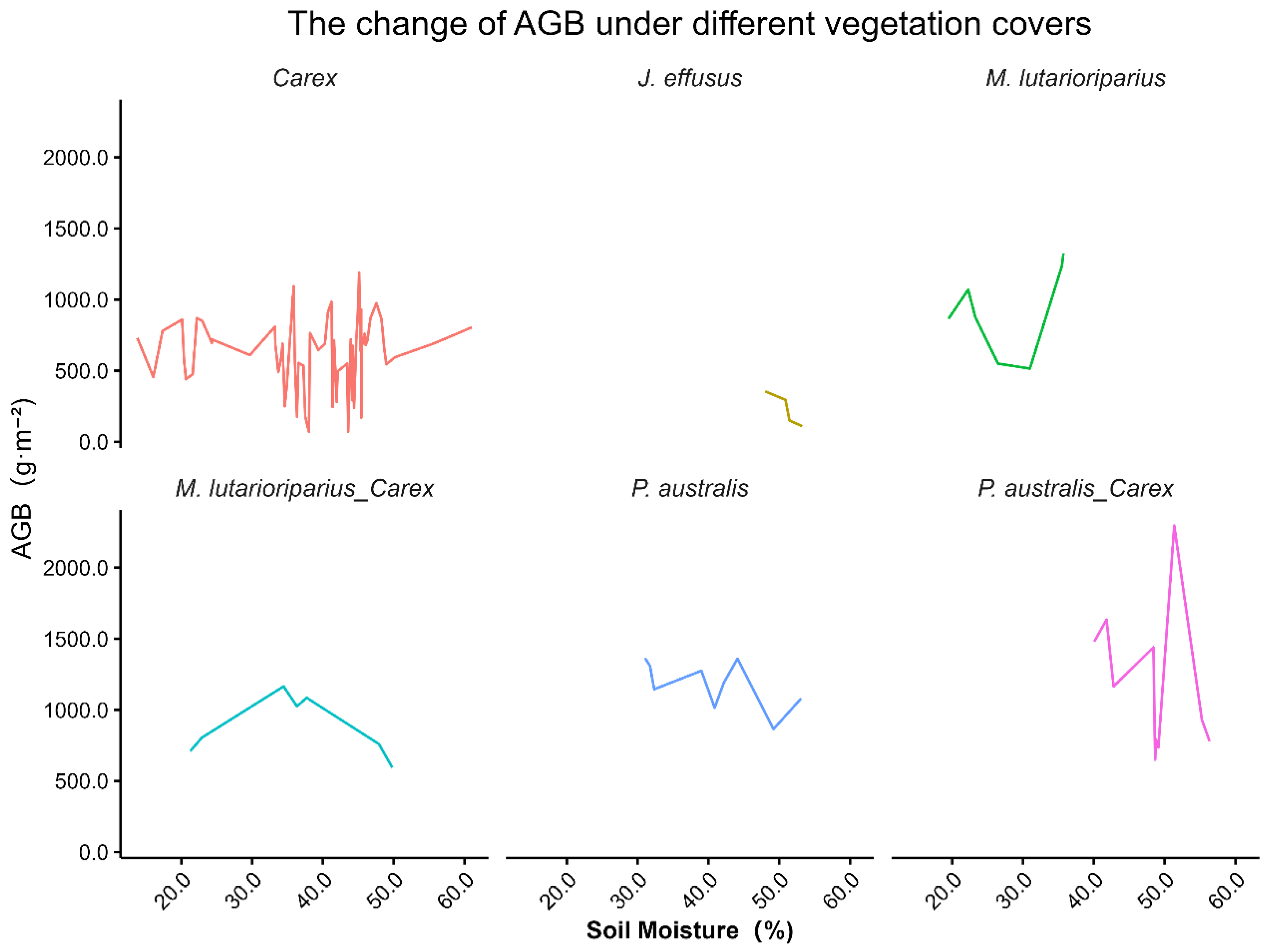
To analyze the AGB characteristics of different vegetation types and understand their environmental adaptability, outliers were excluded prior to analysis to ensure data reliability. Based on sample availability, six representative vegetation types were selected for detailed investigation (Figure 4). The AGB variation of Carex spp. showed no distinct trend in relation to soil moisture. M. lutarioriparius and M. lutarioriparius_Carex exhibited opposite patterns: when soil moisture approached 30%, the AGB of M. lutarioriparius reached its minimum, while that of M. lutarioriparius_Carex was at its maximum. The AGB of P. australis decreased with fluctuations as moisture increased.

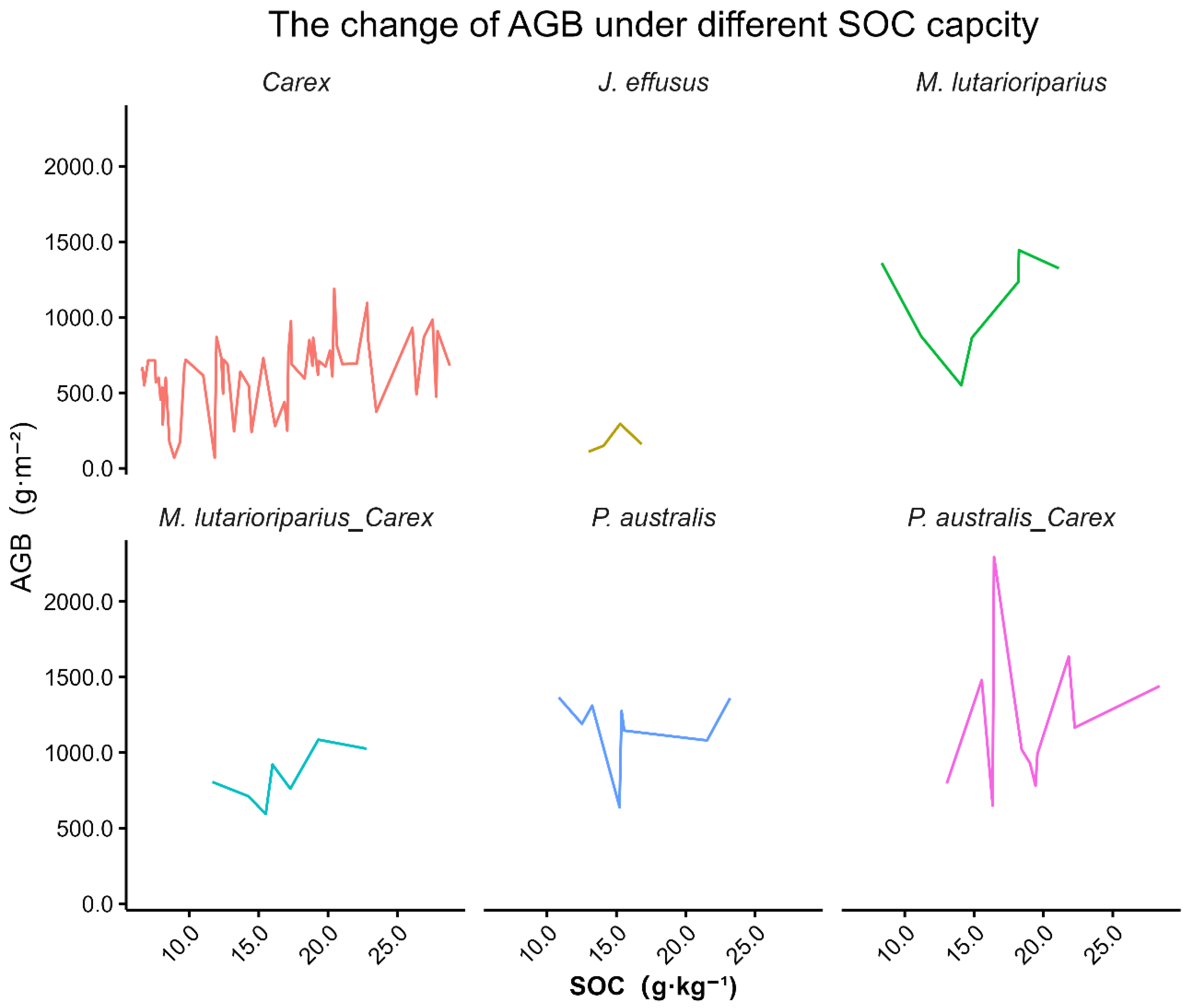
Figure 5 shows the distribution patterns of SOC and AGB for different vegetation types. Carex spp. exhibited the greatest variation in surface SOC content, ranging from 3.99 to 32.71 g·kg⁻¹. Both Carex spp. and M. lutarioriparius_Carex exhibited a pattern where AGB increased with increasing SOC. P. australis _Carex and P. australis did not show a clear trend. J. effusus had the lowest SOC and AGB values.

3.2. Spatial Distribution Characteristics of Vegetation in the Nanji Wetland

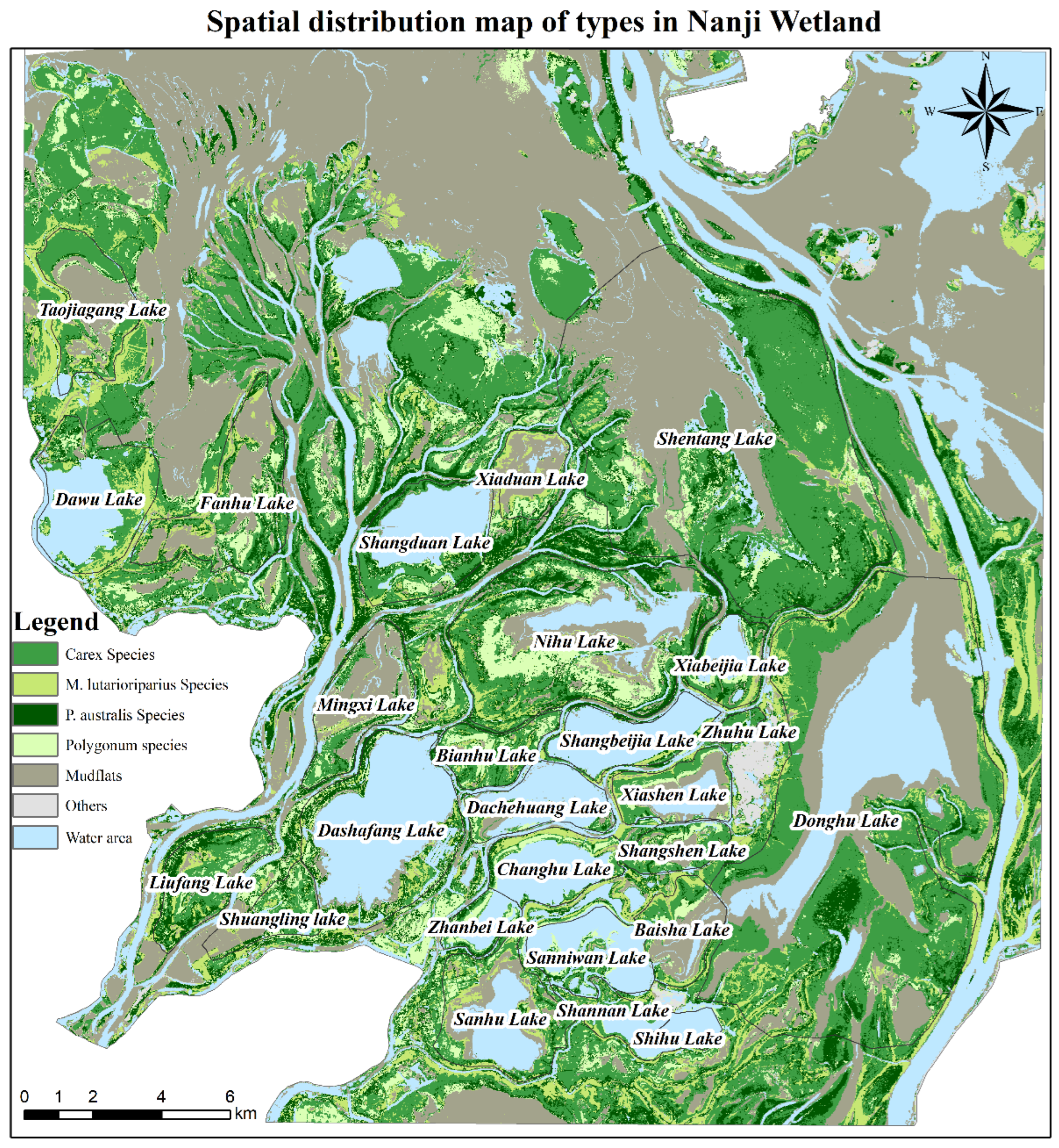
Due to limited sample sizes for certain vegetation types, we classified the wetlands into four main categories: Carex spp., M. lutarioriparius, spp., P. australis spp., and Polygonum spp. (including P. criopolitanum, P. lapathifolium, and P. orientalis). The classification achieved high accuracy (Kappa coefficient = 0.91, OA = 0.92), delineating seven cover types: Carex spp. (219.54 km², 23.75%), M. lutarioriparius, spp. (61.54 km², 6.66%), P. australis spp. (89.93 km², 9.73%), Polygonum spp. (59.26 km², 6.41%), mudflats (292.67 km², 31.65%), water bodies (196.04 km², 21.20%), and other (5.59 km², 0.60%).

The vegetation spatial distribution exhibited distinct ecological zonation (Figure 6). Carex spp. showed the widest distribution, primarily occupying frontal shoals, saucer-shaped lake margins, and mudflat interfaces, while P. australis spp. dominated elevated riverbank shoals. Polygonum spp. preferentially colonised water-adjacent areas of shoals and lakes, and M. lutarioriparius spp. exhibited intermediate distribution between Carex spp. and P. australis. These vegetation types collectively formed characteristic ring- or arc-shaped patterns, reflecting hydrological gradients across the wetland landscape.

3.3. Remote Sensing Inversion Model and Spatial Distribution

3.3.1. Remote Sensing Inversion

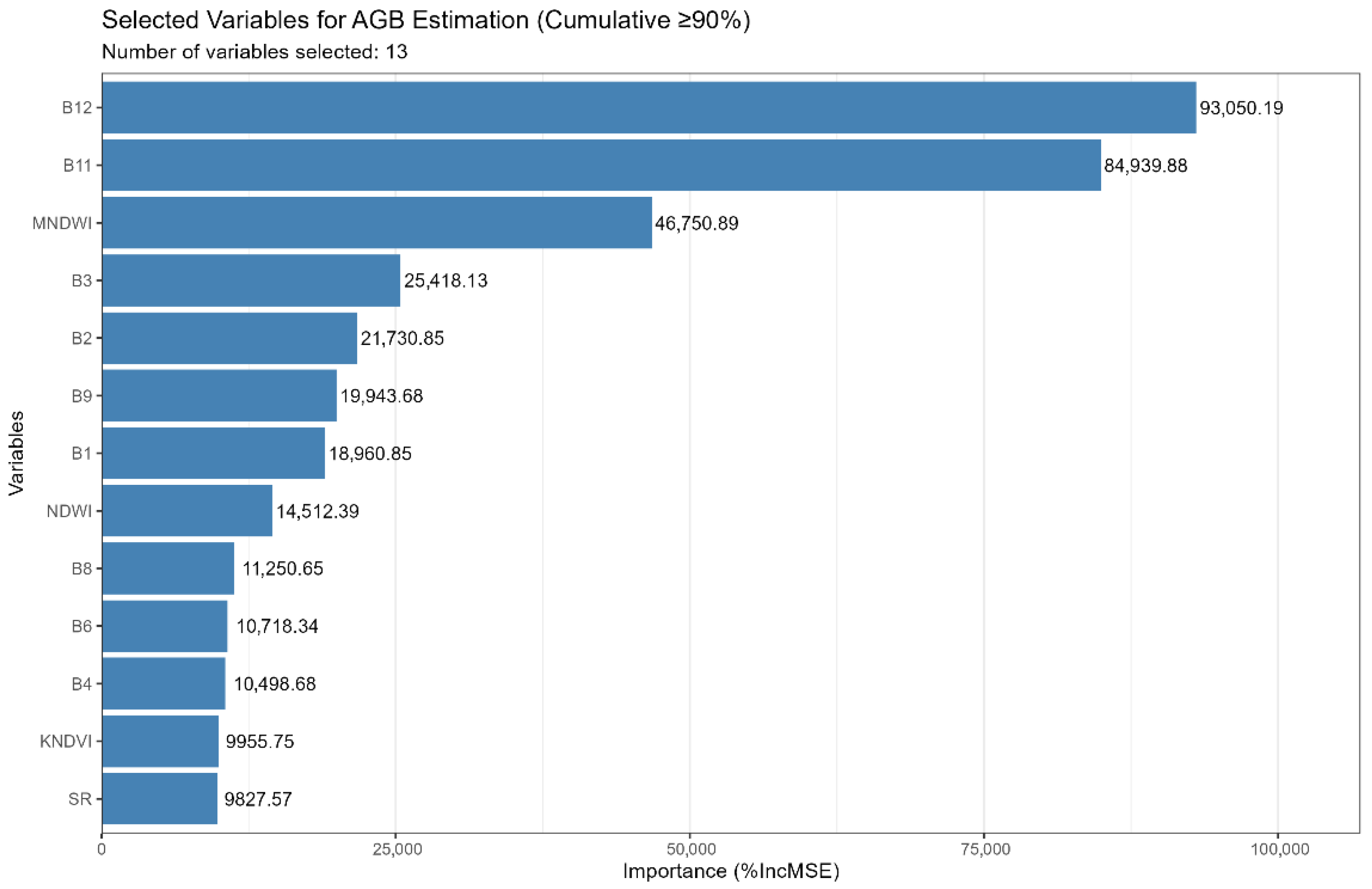
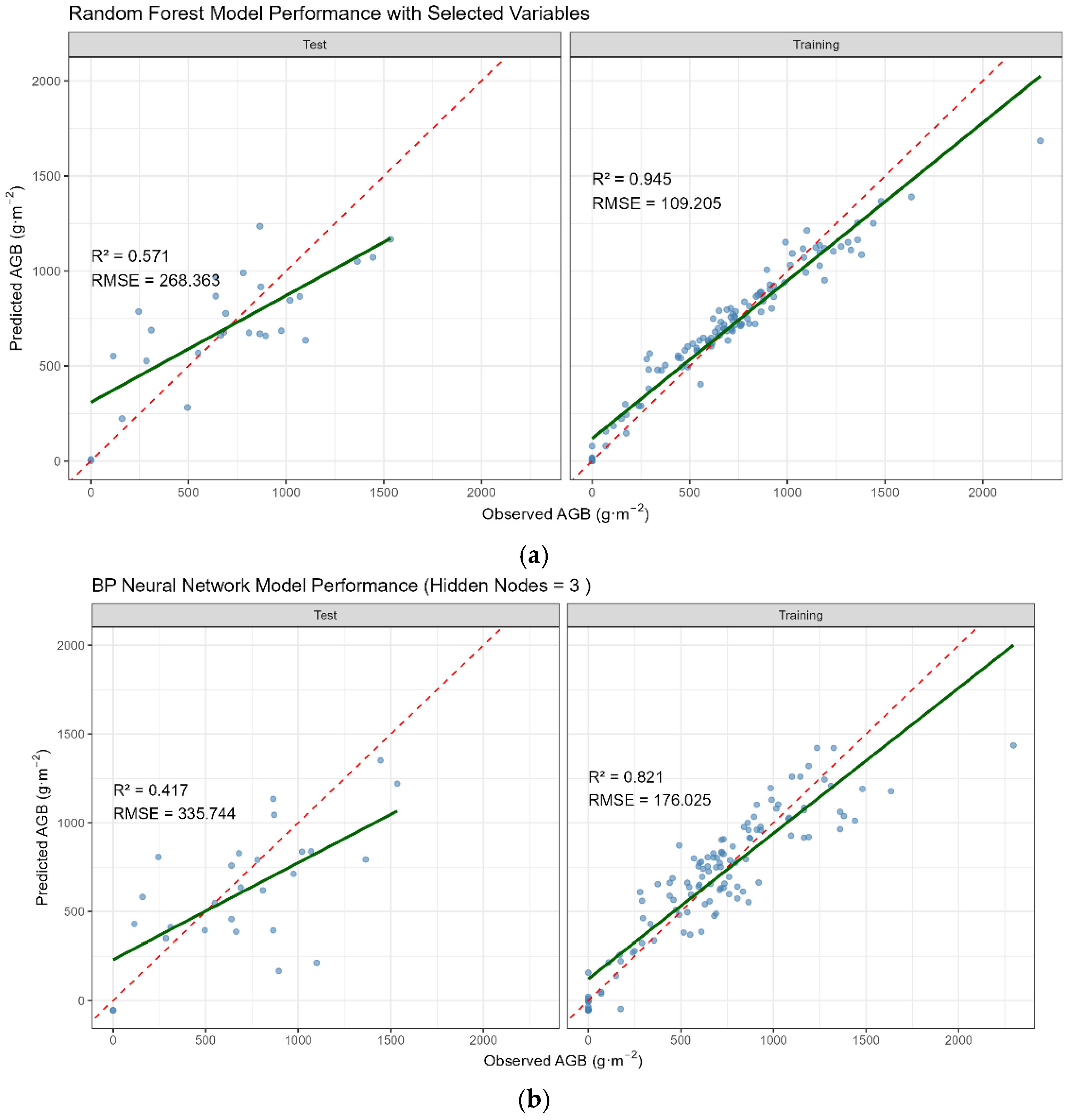
Using R 4.3.3 (R Foundation for Statistical Computing, Vienna, Austria), important variables were first identified based on their cumulative contribution exceeding 90% during variable importance evaluation (Figure 7). Subsequently, regression models for AGB estimation were developed using RF and BPNN algorithms. Comparative analysis of model performance (Figure 8a,b) revealed the superiority of RF. It achieved significantly higher goodness-of-fit than the BPNN on both the training set (R² = 0.945 vs. 0.821) and the validation set (R² = 0.571 vs. 0.417), while also yielding a substantially lower RMSE. Furthermore, RF exhibited a marginally smaller difference in R² between the training and validation sets (ΔR² = 0.374) compared to the BPNN (ΔR² = 0.404). Consequently, RF was selected as the optimal algorithm for AGB estimation.

3.3.2. Spatial Feature Analysis of AGB

Using the established model, we generated AGB predictions through PyCharm 2024.1.2 (JetBrains, Prague, Czechia) and processed the results in ArcGIS 10.2. Water bodies were masked using an NDWI threshold >0, and the resulting AGB distribution was classified using the natural breaks method to produce the spatial distribution map (Figure 9). The Nanji Wetland exhibited relatively high overall biomass, with total AGB reaching 4.03 × 10⁹ g and a mean density of 501.27 g·m⁻². Analysis revealed decreasing AGB gradients from elevated shorelines towards central regions within the saucer-shaped Donghu and Nihu lakes. This spatial characteristic aligns with vegetation distributions along elevation and moisture gradients in the wetland [35,36].

3.3.3. Spatial Distribution Characteristics of Different Vegetation AGB

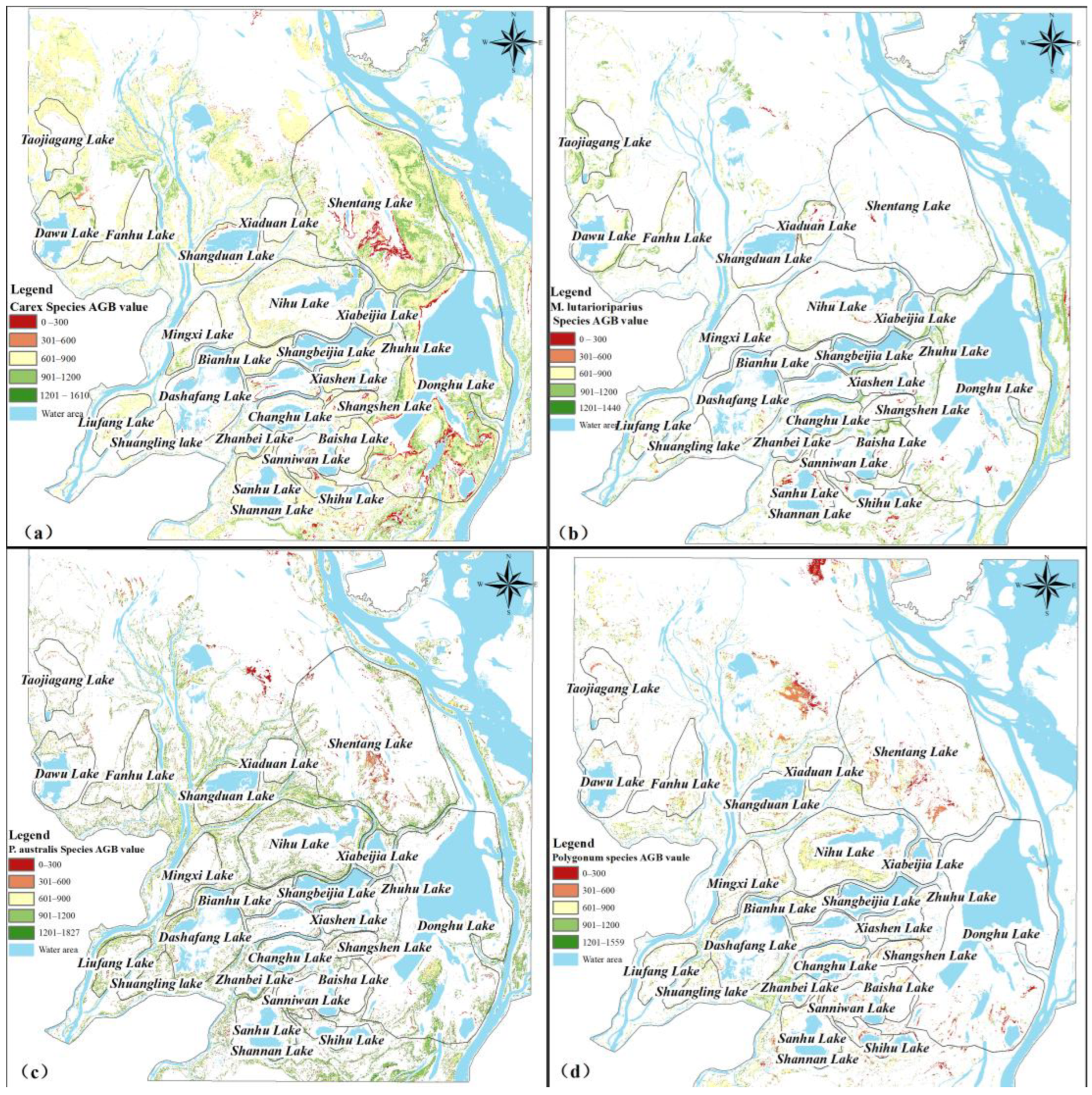
The integration of wetland classification and AGB data revealed distinct biomass distribution patterns among the four vegetation types. Carex spp. exhibited the highest total AGB (1.49 × 10⁹ g), followed by P. australis spp. (6.69 × 10⁸ g), M. lutarioriparius spp. (4.60 × 10⁸ g), and Polygonum spp. (3.61 × 10⁸ g). Mean AGB density decreased in the following order: M. lutarioriparius spp. (859 g·m⁻²) > P. australis spp. (854 g·m⁻²) > Carex spp. (781 g·m⁻²) > Polygonum spp. (700 g·m⁻²). The biomass distribution analysis (

Table 3. Area statistics of AGB for four different types of vegetation.

Unit: km2
Range	Carex		M. lutarioriparius		P. australis		Polygonum
	Area	Ratio	Area	Ratio	Area	Ratio	Area	Ratio
≤300	8.22	4.31%	2.55	4.76%	2.46	3.14%	3.92	7.60%
[301, 600]	7.36	3.85%	1.17	2.18%	4.10	5.24%	7.28	14.13%
[601, 900]	125.82	65.88%	24.05	44.95%	35.99	45.96%	32.45	62.93%
[901, 1200]	47.78	25.02%	25.65	47.95%	34.07	43.52%	7.74	15.02%
≥1201	1.79	0.94%	0.08	0.16%	1.68	2.15%	0.17	0.32%

) indicated that all four vegetation types primarily occurred in the 601–900 g·m⁻² range, with both Carex spp. and Polygonum spp. exceeding 60% representation within this interval. Both M. lutarioriparius spp. and P. australis spp. exceeded 45% representation in each of the two ranges (601–900 g·m⁻² and >901 g·m⁻²), indicating that their biomass levels were consistently high.

The spatial distribution characteristics of AGB for different vegetation types revealed distinct ecological gradients (Figure 10). For Carex spp. (Figure 10a), biomass values show clear zonation characteristics, with lower AGB in mudflat-adjacent areas and higher values in transitional zones between high beaches and mudflats. High-biomass (AGB ≥ 901 g·m⁻²) areas of M. lutarioriparius spp. (Figure 10b) primarily exhibited a linear distribution pattern along elevated lake margins and riverbanks, while low-biomass zones (AGB ≤ 600 g·m⁻²) were dispersed in a scattered pattern. For P. australis spp. (Figure 10c), peak biomass zones likewise primarily occur along elevated lake margins but exhibit more extensive distributional coverage than M. lutarioriparius spp. Polygonum spp. (Figure 10d) primarily occur along lake margins and sandbar fronts. In Nihu Lake, their AGB displays distinct annular zonation decreasing from shore to center, whereas Changhu Lake exhibits parallel linear banding patterns.

4. Discussion

4.1. The Influence of Sampling Time and Area on AGB Estimation Result

Our AGB estimation (4.03 × 10⁹) notably exceeds the results reported by Ye [33] (32.9 × 10⁷ g) but was closer to the result of Yang [18] (6.69 × 10⁹ g in autumn). This discrepancy primarily stems from differences in image resolution—while Ye employed MODIS data (250 m resolution), both our study and that of Yang utilized higher resolution Landsat imagery (30 m). The scale effect of resolution considerably influences ground object representation, where finer resolution better captures small-scale features [49].

Although P. australis spp. typically exhibits higher unit-area biomass due to its tall stems and strong positive correlation with AGB [27], this study found that the mean AGB of M. lutarioriparius spp. was slightly higher than that of P. australis spp. The result was consistent with that of Wan [21], although our absolute values were approximately 38% lower. This discrepancy may arise from differences in elevation and temporal scope. As for elevation, wetland vegetation in Poyang Lake National Nature Reserve occurs above 12 m, while in the Nanji Wetland it is concentrated between 12 and 14 m. The Reserve’s vegetation distribution, particularly at lower elevations, exhibits greater sensitivity to water level fluctuations than the Nanji Wetland [50]. Furthermore, pronounced differences in biomass exist among vegetation types across distinct shallow dish-shaped lakes. Our inversion results (Figure 9) indicate higher AGB values for P. australis spp. than M. lutarioriparius spp., and a paradoxical reversal emerged after spatial averaging across regions. As for temporal scope, this study provides a single-year biomass estimate, whereas Wan used data averaged over 2011–2016. Variations in water level fluctuations across hydrological years, coupled with species-specific inundation tolerance [51] and elevational niches [35], cause regional differences in flood duration, which substantially affect autumn aboveground biomass [52].

4.2. AGB Inversion Variables

By integrating vegetation indices and spectral bands, we mapped the spatial distribution of AGB across four planting types. Interestingly, the RF algorithm identified water indices as the key predictive factor. This contrasts with previous studies that emphasized conventional vegetation indices like SAVI [17], NDVI, and EVI [21] for wetland biomass estimation. This phenomenon can likely be attributed to the sensitivity of wetland vegetation growth to water level fluctuations. Relative to conventional vegetation indices, water indices better capture vegetation growth dynamics and exhibit superior sensitivity in detecting hydrological impacts on plant productivity.

In the Nanji Wetland, plant phenology displays distinct patterns in response to hydrological fluctuations [53]. A clear trend emerges: vegetation typical of higher-elevation zones (e.g., Phragmites australis) is expanding into lower mudflats, while species characteristic of low-lying areas (e.g., Carex spp.) are advancing toward the lake center [54]. These complex dynamics necessitate that AGB inversion for wetland vegetation integrate both changes in surface features captured by remote sensing and variations in growth environments across contrasting hydrological years. Dong [55] confirmed that precipitation has a greater contribution to the AGB than temperature. Arid areas are more sensitive to water availability [56]. For Poyang Lake, the influence of precipitation may be more indirect because the water level of Poyang Lake is jointly affected by rivers. The soil nutrients are particularly important for biomass allocation across different wetland types [57]. A positive feedback mechanism exists between soil nutrients and vegetation, manifested through differential litter decomposition rates across vegetation types and consequent variations in SOC accumulation levels [58]. Therefore, soil moisture should be incorporated as a critical parameter in inversion models in the future, necessitating the integration of continuous field monitoring data from the Nanji Wetland Comprehensive Experimental Station (NWCES) [59].

4.3. Improve the Accuracy of AGB Estimation

This study focuses on the Nanji Wetland, distinguishing vegetation types based on wetland classification to estimate the AGB of its four dominant vegetation types. A key methodological finding arises from comparing aggregated AGB estimates with species-specific ones. The total AGB derived from the broad-scale, non-classified approach (4.03 × 10⁹ g) significantly exceeds the sum obtained from vegetation-specific calculations (2.98 × 10⁹ g). This substantial discrepancy (approximately 1.05 × 10⁹ g) underscores how the inclusion of non-vegetated areas in aggregated models inflates AGB estimates. Consequently, it highlights the critical importance of discriminating vegetation types for achieving accurate biomass assessment, thereby supporting previous research indicating that finer classification granularity enhances estimation accuracy [32]. Although our method obtained relatively fine-grained estimates using remote sensing imagery, it is noteworthy that there was a discrepancy of 0.374 in R² values between the training and test sets. A potential reason may be the uneven sample sizes across different vegetation types, which could lead to model overfitting.

As biomass is a crucial indicator for evaluating regional vegetation carbon sequestration capacity and ecosystem health, finer-scale biomass estimation will improve wetland carbon stock assessments and enable high-precision carbon stock monitoring [60]. A growing number of scholars are utilizing multi-source imagery data, such as Unmanned Aerial Vehicle (UAV) imagery and radar imagery, to conduct high-precision monitoring [61,62,63]. In future studies, in addition to synergizing satellite, aerial, and ground-based data, we will focus on increasing the sample sizes of specific vegetation types rather than merely expanding the total sample size. While this study focused on AGB, belowground biomass (BGB) was not considered. This omission is significant, as previous research within Poyang Lake has demonstrated a U-shaped relationship between water level and biomass allocation patterns for Carex spp. and M. lutarioriparius communities [64]. Furthermore, global wetland surveys emphasize that BGB typically contributes more substantially to soil carbon pools than AGB. This is particularly true for grasses and certain plant orders, which often exhibit high BGB:AGB ratios [65].

5. Conclusions and Outlook

This study compares the inversion performance of the RF and BPNN algorithms for estimating AGB in the Nanji Wetland. Based on the results, the superior-performing RF algorithm was selected for remote sensing inversion using Sentinel-2 imagery, producing the first spatial distribution maps of AGB for four dominant vegetation types. The main findings are summarized below.

(1)

Through important variable evaluation, the spectral bands and indices B12, B11, MNDWI, B3, B2, B9, B1, NDWI, B8, B6, B4, KNDVI, and SR were identified as key predictors for the RF model.

(2)

The key results confirmed RF’s superiority over the BPNN, achieving significantly higher predictive accuracy (R² = 0.945, RMSE = 109.205 g·m⁻²) compared to the BPNN (R² = 0.821, RMSE = 176.025 g·m⁻²).

(3)

During the dry season, the total estimated AGB reached 4.03 × 10⁹ g (mean AGB density = 501.27 g·m⁻²), exhibiting a clear spatial gradient decreasing from higher elevation areas along the lakeshore towards the central lake regions. Among the vegetation types, Carex spp. dominated AGB accumulation (1.49 × 10⁹ g), significantly surpassing P. australis spp. (6.69 × 10⁸ g), M. lutarioriparius spp. (4.60 × 10⁸ g), and Polygonum spp. (3.61 × 10⁸ g). However, in terms of mean AGB density per unit area, M. lutarioriparius spp. exhibited the highest value (859 g·m⁻²), slightly exceeding that of P. australis spp. (854 g·m⁻²), Carex spp. (781 g·m⁻²), and Polygonum spp. (700 g·m⁻²).

This study focuses on the fine-scale estimation of AGB in the Nanji Wetland and reveals the spatial distribution characteristics of four vegetation types. However, the research is subject to the following limitations:

(1)

Exclusion of belowground and aquatic vegetation biomass. BGB and aquatic vegetation biomass were not considered. Future studies aiming for precise regional carbon stock estimation should incorporate both AGB and BGB across terrestrial vegetation, as well as biomass from aquatic vegetation.

(2)

Limited environmental variables in the inversion process. The inversion model did not incorporate a broader range of environmental variables known to correlate with biomass. To achieve more accurate biomass estimation in the future, variables influencing biomass dynamics, such as soil properties and hydrological conditions, need to be integrated.

(3)

Lack of investigation into hydrological regulation pathways. The pathway through which hydrological regulation policies influence biomass was not explored. Future research should investigate the spatial dynamics of overall Poyang Lake biomass under different hydrological management regimes. This knowledge is essential for enhancing the lake’s carbon sequestration capacity through scientifically informed hydrological regulation.

References

1. Dayathilake, D.D.T.L.; Lokupitiya, E.; Wijeratne, V.P.I.S. Estimation of aboveground and belowground carbon stocks in urban freshwater wetlands of Sri Lanka. Carbon Balance Manag. 2020, 15, 17. [Google Scholar] [CrossRef]
2. Ray, R.; Ganguly, D.; Chowdhury, C.; Dey, M.; Das, S.; Dutta, M.K.; Mandal, S.K.; Majumder, N.; De, T.K.; Mukhopadhyay, S.K.; et al. Carbon sequestration and annual increase of carbon stock in a mangrove forest. Atmos. Environ. 2011, 45, 5016–5024. [Google Scholar] [CrossRef]
3. Becknell, J.M.; Kucek, L.K.; Powers, J.S. Aboveground biomass in mature and secondary seasonally dry tropical forests: A literature review and global synthesis. For. Ecol. Manag. 2012, 276, 88–95. [Google Scholar] [CrossRef]
4. Estrada, G.C.; Soares, M.L. Global patterns of aboveground carbon stock and sequestration in mangroves. An. Acad. Bras. Ciênc. 2017, 89, 973–989. [Google Scholar] [CrossRef] [PubMed]
5. Sun, S.; Wang, Y.; Song, Z.; Chen, C.; Zhang, Y.; Chen, X.; Chen, W.; Yuan, W.; Wu, X.; Ran, X.; et al. Modelling aboveground biomass carbon stock of the Bohai Rim coastal wetlands by integrating remote sensing, terrain, and climate data. Remote Sens. 2021, 13, 4321. [Google Scholar] [CrossRef]
6. Wang, Y.; Shen, X.; Tong, S.; Zhang, M.; Jiang, M.; Lu, X. Aboveground biomass of wetland vegetation under climate change in the western Songnen plain. Front. Plant Sci. 2022, 13, 941689. [Google Scholar] [CrossRef]
7. Zhou, L.; Yan, W.; Sun, X.; Shao, J.; Zhang, P.; Zhou, G.; He, Y.; Liu, H.; Fu, Y.; Zhou, X. Regulation of climate, soil and hydrological factors on macrophyte biomass allocation for coastal and inland wetlands in China. Sci. Total Environ. 2021, 774, 145317. [Google Scholar] [CrossRef]
8. Yao, Y.; Ren, H. Estimation of grassland aboveground biomass on the Qinghai-Tibet Plateau. Acta Ecol. Sin. 2024, 44, 3049–3059. [Google Scholar]
9. Zang, P.; Zhang, Y.; Chen, Z.; Hou, G.; Liu, Z.; Lu, X. The inversion modeling and aboveground biomass mapping of withered grass changes in the western grassland of Northeast China. Front. Earth Sci. 2023, 10, 1031098. [Google Scholar] [CrossRef]
10. Jin, X.; Lou, Y.; Zhang, P.; Tang, H.; Zhang, Q.; Smith, P. Allometric equations for estimating above-and below-ground biomass of reed (Phragmites australis) marshes. J. Plant Ecol. 2025, 18, rtae113. [Google Scholar] [CrossRef]
11. Jensen, D.; Cavanaugh, K.C.; Simard, M.; Christensen, A.; Rovai, A.; Twilley, R. Aboveground biomass distributions and vegetation composition changes in Louisiana’s Wax Lake Delta. Estuar. Coast. Shelf Sci. 2021, 250, 107139. [Google Scholar] [CrossRef]
12. Liu, Y.; Shen, X.; Wang, Y.; Zhang, J.; Ma, R.; Lu, X.; Jiang, M. Spatiotemporal variation in aboveground biomass and its response to climate change in the marsh of Sanjiang Plain. Front. Plant Sci. 2022, 13, 920086. [Google Scholar] [CrossRef]
13. Ren, Y.; Mao, D.; Li, X.; Wang, Z.; Xi, Y.; Feng, K. Aboveground biomass of marshes in Northeast China: Spatial pattern and annual changes responding to climate change. Front. Ecol. Evol. 2022, 10, 1043811. [Google Scholar] [CrossRef]
14. Lv, G.; Cui, G.; Wang, X.; Yu, H.; Huang, X.; Zhu, W.; Lin, Z. Signatures of wetland impact: Spatial distribution of forest aboveground biomass in Tumen River Basin. Remote Sens. 2021, 13, 3009. [Google Scholar] [CrossRef]
15. Lan, Z.; Chen, Y.; Shen, R.; Cai, Y.; Luo, H.; Jin, B.; Chen, J. Effects of flooding duration on wetland plant biomass: The importance of soil nutrients and season. Freshw. Biol. 2021, 66, 211–222. [Google Scholar] [CrossRef]
16. Zhou, Z.; Yang, Y.; Chen, B. Estimating Spartina alterniflora fractional vegetation cover and aboveground biomass in a coastal wetland using SPOT6 satellite and UAV data. Aquat. Bot. 2018, 144, 38–45. [Google Scholar] [CrossRef]
17. Rao, D.; Yu, X.; Li, P.; Xia, S.; Meng, Z.; Liu, Y. Remote sensing estimation of spring Carex biomass in Changhuchi Lake, a shallow sub-lake of Poyang Lake. J. Nat. Resour. 2019, 34, 2001–2011. [Google Scholar] [CrossRef]
18. Yang, L.; Xieqin, M.; Li, Q.; Zhang, X.; Zhu, J.; Gao, J. Spatial and temporal dynamics of plant biomass in Poyang Lake Wetland in Spring and Autumn in recent two decades. J. Changjiang River Sci. Res. 2024, 41, 47–54. [Google Scholar]
19. Berdugo, M.; Delgado-Baquerizo, M.; Soliveres, S.; Hernández-Clemente, R.; Zhao, Y.; Gaitán, J.J.; Gross, N.; Saiz, H.; Maire, V.; Lehman, A.; et al. Global ecosystem thresholds driven by aridity. Science 2020, 367, 787–790. [Google Scholar] [CrossRef]
20. Li, C.; Zhou, L.; Xu, W. Estimating aboveground biomass using Sentinel-2 MSI data and ensemble algorithms for grassland in the Shengjin Lake Wetland, China. Remote Sens. 2021, 13, 1595. [Google Scholar] [CrossRef]
21. Wan, R.; Wang, P.; Wang, X.; Yao, X.; Dai, X. Mapping aboveground biomass of four typical vegetation types in the Poyang Lake wetlands based on random forest modelling and Landsat images. Front. Plant Sci. 2019, 10, 1281. [Google Scholar] [CrossRef]
22. Li, H.; Li, F.; Xiao, J.; Chen, J.; Lin, K.; Bao, G.; Liu, A.; Wei, G. A machine learning scheme for estimating fine-resolution grassland aboveground biomass over China with Sentinel-1/2 satellite images. Remote Sens. Environ. 2024, 311, 114317. [Google Scholar] [CrossRef]
23. Lyu, X.; Li, X.; Gong, J.; Li, S.; Dou, H.; Dang, D.; Xuan, X.; Wang, H. Remote-sensing inversion method for aboveground biomass of typical steppe in Inner Mongolia, China. Ecol. Indic. 2021, 120, 106883. [Google Scholar] [CrossRef]
24. Yang, X.; Man, W.; Liu, M.; Zhang, Y.; Zheng, H.; Song, J.; Kang, Z. Estimation model of Spartina alterniflora aboveground biomass by remote sensing in Zhejiang Coastal Wetland. Remote Sens. Technol. Appl. 2023, 38, 1445–1454. [Google Scholar]
25. Zhou, R.; Yang, C.; Li, E.; Cai, X.; Wang, X. Aboveground biomass estimation of wetland vegetation at the species level using unoccupied aerial vehicle RGB imagery. Front. Plant Sci. 2023, 14, 1181887. [Google Scholar] [CrossRef]
26. Adam, E.; Mutanga, O.; Abdel-Rahman, E.M.; Ismail, R. Estimating standing biomass in papyrus (Cyperus papyrus L.) swamp: Exploratory of in situ hyperspectral indices and random forest regression. Int. J. Remote Sens. 2014, 35, 693–714. [Google Scholar] [CrossRef]
27. Xi, M.; Kong, F.; Feng, X.; Zi, Y.; Li, Y. Growth dynamics and empirical formula for biomass evaluation of aboveground part of Phragmites australis in Jiaozhou Bay Wetlands. Wetl. Sci. 2016, 14, 816–824. [Google Scholar]
28. Wang, S.; Li, S.; Zheng, S.; Gao, W.; Zhang, Y.; Cao, B.; Cui, B.; Shao, D. Estimating biomass and carbon sequestration capacity of Phragmites australis using remote sensing and growth dynamics modeling: A case study in Beijing Hanshiqiao wetland nature reserve, China. Sensors 2022, 22, 3141. [Google Scholar] [CrossRef]
29. Zhao, Y.; Mao, D.; Zhang, D.; Wang, Z.; Du, B.; Yan, H.; Qiu, Z.; Feng, K.; Wang, J.; Jia, M. Mapping Phragmites australis aboveground biomass in the momoge wetland ramsar site based on Sentinel-1/2 images. Remote Sens. 2022, 14, 694. [Google Scholar] [CrossRef]
30. Wu, N.; Zhang, C.; Zhuo, W.; Shi, R.; Zhu, F.; Liu, S. Assessment of the impact of coastal wetland saltmarsh vegetation types on aboveground biomass inversion. Remote Sens. 2024, 16, 4762. [Google Scholar] [CrossRef]
31. Xu, Y.; Qin, Y.; Li, B.; Li, J. Estimating vegetation aboveground biomass in Yellow River Delta coastal wetlands using Sentinel-1, Sentinel-2 and Landsat-8 imagery. Ecol. Inform. 2025, 87, 103096. [Google Scholar] [CrossRef]
32. Zhao, T.; Yu, R.; Zhang, Z.; Bai, X.; Zeng, Q. Estimation of wetland vegetation aboveground biomass based on remote sensing data: A review. Chin. J. Ecol. 2016, 35, 1936–1946. [Google Scholar]
33. Ye, C.; Zhao, X.; Wu, G.; Wang, X.; Liu, Y. Vegetation biomass spatial-temporal variations and the influence of the water level in Poyang Lake National Nature Reserve. J. Lake Sci. 2013, 25, 707–714. [Google Scholar] [CrossRef] [PubMed]
34. Xie, D.; Huang, Q.; Yi, Q.; Zhu, Z.; Zhou, G.; Tian, L.; Zhou, Y.; Jia, J.; Qian, H. Changes in floodplain vegetation in Poyang Lake wetlands. Acta Ecol. Sin. 2019, 39, 4070–4079. [Google Scholar]
35. Tan, Z.; Zhang, Q.; Li, Y.; Xu, X.; Jiang, J. Distribution of typical vegetation communities along elevation in Poyang Lake Wetlands. Wetl. Sci. 2016, 14, 506–515. [Google Scholar]
36. Zhang, Q.; Yu, X.; Hu, B. Research on the characteristics of plant communities in the Poyang Nanji Wetlands, China. Resour. Sci. 2013, 35, 42–49. [Google Scholar]
37. Guo, R.; Fu, S.; Hou, M.; Liu, J.; Miao, C.; Meng, X.; Feng, Q.; He, J.; Qian, D.; Liang, T. Remote sensing retrieval of nature grassland biomas in Menyuan County, Qinghai Province experimental area based on Sentinel-2 data. Acta Prataculturae Sin. 2023, 32, 15–29. [Google Scholar]
38. Ge, G.; Wu, L. Analysis on the Flora of Seed Plants in Nanjishan Nature Reserve Jiangxi. J. Nanchang Univ. 2006, 30, 52–55. [Google Scholar]
39. Zhi, Y.; Yi, J.; Liu, W.; Gong, H.; Shao, M.; Dai, N.; Li, Q.; Yang, W. Monitoring of wintering waterbirds in the Nanji Wetland National Nature Reserve of Poyang Lake. Chin. J. Ecol. 2020, 39, 2400–2407. [Google Scholar]
40. Forzieri, G.; Dakos, V.; McDowell, N.G.; Ramdane, A.; Cescatti, A. Emerging signals of declining forest resilience under climate change. Nature 2022, 608, 534–539. [Google Scholar] [CrossRef]
41. Breiman, L. Random Forests. Mach. Learn. 2001, 45, 5–32. [Google Scholar] [CrossRef]
42. Sheykhmousa, M.; Mahdianpari, M.; Ghanbari, H.; Mohammadimanesh, F.; Ghamisi, P.; Homayouni, S. Support vector machine versus random forest for remote sensing image classification: A meta-analysis and systematic review. IEEE J. Sel. Top. Appl. Earth Obs. Remote Sens. 2020, 13, 6308–6325. [Google Scholar] [CrossRef]
43. Schonlau, M.; Zou, R.Y. The random forest algorithm for statistical learning. Stata J. 2020, 20, 3–29. [Google Scholar] [CrossRef]
44. Liang, S.; Cheng, J.; Jia, K.; Jiang, B.; Liu, Q.; Liu, S.; Xiao, Z.; Xie, X.; Yao, Y.; Yuan, W. Recent progress in land surface quantitative remote sensing. J. Remote Sens. 2016, 20, 875–898. [Google Scholar]
45. Li, H.; Tang, X.; Cui, L.; Zhai, X.; Wang, J.; Zhao, X.; Li, J.; Lei, Y.; Wang, J.; Wang, R.; et al. Estimating aboveground biomass of wetland plant communities from hyperspectral data based on fractional-order derivatives and machine learning. Remote Sens. 2024, 16, 3011. [Google Scholar] [CrossRef]
46. Rumelhart, D.; Hinton, G.E.; Williams, R.J. Learning representations by Back Propagating Errors. Nature 1986, 323, 533–536. [Google Scholar] [CrossRef]
47. Zhang, G.; Chen, D.; Li, H.; Pei, M.; Zhen, Q.; Zheng, J.; Zhao, H.; Hu, Y.; Fan, J. Estimation of aboveground biomass of Picea schrenkiana forests considering vertical zonality and stand age. Forests 2025, 16, 445. [Google Scholar] [CrossRef]
48. Yu, X.; Wang, J.; Xia, Y.; Liu, J.; Chen, Y. Study on the influence of nutritional status of disc lake on Carex. Ecol. Sci. 2024, 43, 85–90. [Google Scholar]
49. Zhang, B.; Liu, Q.; Li, X.; Liu, L.; Yang, B.; Husi, L.; Gao, L.; Zhang, W.; Zhang, H.; Bian, Z. The core concepts and fundamental issues of remote sensing science. Natl. Remote Sens. Bull. 2025, 29, 1–48. [Google Scholar] [CrossRef]
50. Liu, X.; Guan, Y.; Guo, S.; Zhang, C.; Wang, L. Response on wetland vegetation distribution to hydrology regularity based on harmonic-time series analysis. J. Lake Sci. 2016, 28, 12. [Google Scholar] [CrossRef]
51. Wang, R.; Peng, W.; Liu, X.; Wu, W.; Han, Z.; Jiang, C. Analysis of responses of typical vegetation in Nanji Wetland National Nature Reserve of Poyang Lake to water depth and submergence frequency. J. China Inst. Water Resour. Hydropower Res. 2018, 6, 528–535. [Google Scholar]
52. Zhao, Y.; Wen, Y.; Wang, F.; Cui, X.; Lan, Z.; Cai, Y.; Zhang, Y.; Lu, S. The effect of flooding duration on the vegetation biomass allocation pattern in shallow lakes of Poyang Lake. J. Jiangxi Norm. Univ. 2024, 48, 572–579. [Google Scholar]
53. Zhang, L.; Luo, W.; Zhang, H.; Yin, X.; Li, B. Classification scheme for mapping wetland herbaceous plant communities using time series Sentinel-1 and Sentinel-2 data. Natl. Remote Sens. Bull. 2023, 27, 1362–1375. [Google Scholar] [CrossRef]
54. Lin, Y.; Li, X.; Tan, Z.; Song, Y.; Xu, C. Dynamic characteristics of vegetation communities in the floodplain wetland of Lake Poyang based on spatio-temporal fusion of remote sensing data. J. Lake Sci. 2023, 35, 1408–1422. [Google Scholar] [CrossRef]
55. Dong, P.; Jing, C.; Wang, G.; Shao, Y.; Gao, Y. The Estimation of Grassland Aboveground Biomass and Analysis of Its Response to Climatic Factors Using a Random Forest Algorithm in Xinjiang, China. Plants 2024, 13, 548. [Google Scholar] [CrossRef] [PubMed]
56. Liu, D.; Zhang, C.; Ogaya, R.; Fernández-Martínez, M.; Pugh, T.; Peuelas, J. Increasing climatic sensitivity of global grassland vegetation biomass and species diversity correlates with water availability. New Phytol. 2021, 230, 1761–1771. [Google Scholar] [CrossRef]
57. Pan, Y.; Zhang, Z.; Liu, M. Climate vs. nutrient control: A global analysis of driving environmental factors of wetland plant biomass allocation strategy. J. Clean. Prod. 2023, 406, 136983. [Google Scholar] [CrossRef]
58. Zhang, Q.; Yu, X.; Zhang, G. Variation characteristics of the decomposition process δ13C and δ15 N of three dominant plant litter in Lake Poyang wetland. J. Lake Sci. 2023, 35, 1694–1704. [Google Scholar]
59. Huang, Q.; Fang, C.; Hu, Q. Progresses of wetland ecosystem field monitoring in Nanji Wetland National Nature Reserve, South of Poyang Lake. Wetl. Sci. 2017, 15, 8. [Google Scholar]
60. Liu, Y.; Feng, T.; Chen, B. Estimation of multi-scale biomass and carbon storage in the coastal wetlands of Ningbo City through Filed-UAV-Satellite synergy. Natl. Remote Sens. Bull. 2025, 29, 147–166. [Google Scholar] [CrossRef]
61. Doughty, C.L.; Ambrose, R.F.; Okin, G.S.; Cavanaugh, K.C. Characterizing spatial variability in coastal wetland biomass across multiple scales using UAV and satellite imagery. Remote Sens. Ecol. Conserv. 2021, 7, 411–429. [Google Scholar] [CrossRef]
62. Tang, Y.; Ma, J.; Xu, J.; Wu, W.; Wang, Y.; Guo, H. Assessing the impacts of tidal creeks on the spatial patterns of coastal salt marsh vegetation and its aboveground biomass. Remote Sens. 2022, 14, 1839. [Google Scholar] [CrossRef]
63. Naidoo, L.; Van Deventer, H.; Ramoelo, A.; Mathieu, R.; Nondlazi, B.; Gangat, R. Estimating above ground biomass as an indicator of carbon storage in vegetated wetlands of the grassland biome of South Africa. Int. J. Appl. Earth Obs. Geoinf. 2019, 78, 118–129. [Google Scholar] [CrossRef]
64. Yang, J.; Hu, Q.; Liu, Y.; Ye, J.; Liu, H.; Huang, L.; Yao, B. Responses of plant biomass and allocation to plant diversity changes in typical wetlands of Poyang Lake. Chin. J. Appl. Environ. Biol. 2023, 29, 1337–1345. [Google Scholar]
65. Pan, Y.; Liu, J.; Zhang, M.; Huang, P.; Hipesy, M.; Dai, L.; Ma, Z.; Zhang, F.; Zhang, Z. The below-ground biomass contributes more to wetland soil carbon pools than the above-ground biomass—A survey based on global wetlands. J. Plant Ecol. 2024, 17, rtae017. [Google Scholar] [CrossRef]
Figure 1. Location of the research area and sample points distribution ((a) location of Poyang Lake, (b) Location of the research area., (c) The sample points distribution map).
Forests 16 01376 g001
Figure 2. The framework of the BPNN (cited from Zhang [47]).
Forests 16 01376 g002
Figure 3. The research roadmap.
Forests 16 01376 g003
Figure 4. Soil moisture changes of different vegetation under different elevations.
Forests 16 01376 g004
Figure 5. SOC characteristics of different vegetation distribution heights and topsoil.
Forests 16 01376 g005
Figure 6. Wetland classification results.
Forests 16 01376 g006
Figure 7. The cumulative contribution of important variables.
Forests 16 01376 g007
Figure 8. (a) Test and training result graphs of AGB with the RF model; (b) test and training result graphs of AGB with the BPNN model.
Forests 16 01376 g008
Figure 9. Spatial distribution of AGB.
Forests 16 01376 g009
Figure 10. Spatial distribution maps of AGB for four types of vegetation ((a) Carex spp., (b) M. lutarioriparius spp., (c) P. australis spp., and (d) Polygonum spp.).
Forests 16 01376 g010