Abstract
Abies nebrodensis L. is a critically endangered conifer endemic to Sicily (Italy). Its residual population is confined to the Madonie mountain range under challenging climatological conditions. Despite the good adaptation shown by the relict population to the environmental conditions occurring in its habitat, Abies nebrodensis is subject to a series of threats, including climate change. Effective conservation strategies require reliable and versatile methods for monitoring its health status. Combining high-resolution remote sensing data with reanalysis of climatological datasets, this study aimed to identify correlations between vegetation indices (NDVI, GreenDVI, and EVI) and key climatological variables (temperature and precipitation) using advanced machine learning techniques. High-resolution RGB (Red, Green, Blue) and IrRG (infrared, Red, Green) maps were used to delineate tree crowns and extract statistics related to the selected vegetation indices. The results of phytosanitary inspections and multispectral analyses showed that the microclimatic conditions at the site level influence both the impact of crown disorders and tree physiology in terms of water content and photosynthetic activity. Hence, the correlation between the phytosanitary inspection results and vegetation indices suggests that multispectral techniques with drones can provide reliable indications of the health status of Abies nebrodensis trees. The findings of this study provide significant insights into the influence of environmental stress on Abies nebrodensis and offer a basis for developing new monitoring procedures that could assist in managing conservation measures.
1. Introduction
Monitoring is a critical component in the management and conservation of endangered species, providing essential data for evaluating their conservation status and identifying vulnerability factors that could influence population dynamics [1]. Through the systematic collection of data, monitoring can assist in assessing ecological health, identifying priority interventions, and supporting informed decision-making for conservation planning and policy implementation for the conservation of ecosystems [2].
Among the endangered species, Abies nebrodensis (Lojac.) Mattei, commonly known as Sicilian fir, a Mediterranean fir endemic to northern Sicily (Italy), is of particular interest. This species is listed in the IUCN (Red List of Threatened Species) [3] and is classified as “critically endangered” under criteria A2cd. With its natural population reduced to only 30 relict trees, Sicilian fir is the rarest conifer in Europe [4]. The limited distribution of A. nebrodensis is a result of the historical overexploitation that persisted until the 19th century, which led to a significant decline in its population size and genetic diversity [4,5]. The great vulnerability of this species is due to genetic erosion, a high rate of self-fertilization, poor natural regeneration, the impact of the supernumerary populations of fallow deer and wild boars, and possible hybridization with non-native firs planted nearby in the past [6,7]. In addition, the effects of climate change may be highly detrimental for this endangered species, affecting plant growth and vigor, altering its phenology, and impairing physiological processes. Environmental stresses can also predispose trees to pests and pathogen attacks, potentially leading to further population decline [8,9]. The impact of crown disorders on A. nebrodensis trees was assessed and was found to be related to the environmental conditions the trees were facing at the microclimate and site levels [8]. The same study provided insights into the phyllosphere fungal community associated with the observed disorders, but surveys on the physiological state of the trees have not yet been conducted.
A recent study [10] showed that among the circum-Mediterranean firs, A. nebrodensis is the species that could suffer a loss of suitable area in the harshest scenario.
Over the past two decades, Italy has experienced a notable increase in extreme meteorological and climatic events, significantly impacting its environment, economy, and public health. The frequency and intensity of heatwaves, floods, droughts, and other severe weather phenomena have escalated [11,12,13].
According to the European Severe Weather Database [14] (ESWD, accessed on 3 January 2025), Italy was hit by 539 extreme weather events from January 2020 to December 2024 (query related to “large hail”, “heavy rain”, and “severe wind gust” events). The increasing frequency of these extreme events has profound implications for natural ecosystems, agriculture, and biodiversity. Prolonged droughts and heat stress have adversely affected crop yields and forest health, while intense storms and flooding have led to soil erosion and habitat degradation [15,16]. For these reasons, there is an urgent need to monitor the environmental stressors that may alter biodiversity, with a particular focus on rare and endangered species.
Conservation initiatives have been implemented to mitigate these threats and safeguard the remaining population of Sicilian fir. Among these initiatives, the LIFE4FIR project (LIFE18 NAT/IT/000164) aimed to enhance the conservation status of this critically endangered species through a combination of in situ and ex situ interventions. Phytosanitary monitoring has been an integral part of these efforts, providing valuable insights into tree health and serving as a baseline for evaluating future changes. Traditional ground-based assessments, although informative, may have limitations in terms of spatial coverage, efficiency, and consistency, highlighting the need for advanced remote sensing technologies to complement field observations. Integrating advanced remote sensing technologies, such as Unmanned Aerial Vehicle (UAV)-acquired multispectral imaging, with long-term climatic data analysis can enhance our understanding of environmental impacts and assist in adopting effective conservation measures for vulnerable species and ecosystems [17,18,19]. UAV-based multispectral imaging enables the acquisition of high-resolution data across multiple spectral bands, facilitating the detection of subtle changes in vegetation health that may not be visible to the naked eye. This technology allows for the calculation of vegetation indices that are indicative of plant physiological status, such as the Normalized Difference Vegetation Index (NDVI), Enhanced Vegetation Index (EVI), red-edge NDVI, and Excess Green Index (ExGreen). These indices have been widely used to monitor vegetation stress, detect disease outbreaks, and assess the impact of environmental factors on plant health [19,20].
The present study aims to develop an advanced remote sensing technique for analyzing and classifying the health status of Sicilian fir trees in their natural habitat using UAV-acquired multispectral images, as well as constructing a classification model for plant health status.
In addition to spectral analysis, this study investigates how ongoing climate changes are affecting the habitat of firs using historical climatological data collected from the ERA5-Land datasets.
By combining multispectral UAV data with long-term climatic trends and phytosanitary surveys, this study provides a comprehensive understanding of the factors driving the health status and vulnerability of Sicilian fir. This integrative approach will enable conservation managers to develop targeted strategies for mitigating the impact of climate change and other stressors on the species.
2. Materials and Methods
2.1. Methodological Approach
To analyze the acquired UAV imagery, features related to the tree crowns were first reconstructed using Geographic Information System (GIS) techniques. Multispectral images were then overlaid with vector-based crown delineations to extract spectral values specific to each tree. The extracted spectral data were used to compute the vegetation indices, whose frequency distributions were used for training machine learning models to classify tree health conditions.
Furthermore, this study employed advanced statistical analyses to assess the relationship between the vegetation indices and known health indicators, aiming to establish a reliable remote sensing framework for long-term monitoring. The integration of climatic and meteorological data with multispectral analysis provided insights into the potential correlation between observed disorders and climate-induced stress factors.
2.2. Study Area
The residual range of the Sicilian fir (A. nebrodensis) is located in the municipality of Polizzi Generosa (Palermo, Sicily, Italy) and lies in the Madonie Regional Park, which covers an area of 40,000 hectares in the north–central part of Sicily (southern Italy). The study area is bounded by the following coordinates: upper-left: 14°0′52″ E, 37°50′52″; upper-right: 14°2′36″ E, 37°50′52″; bottom-right: 14°2′36″ E, 37°49′49″; and bottom-left: 14°0′52″ E, 37°50′52″ (coordinate system: WGS84–WebMercator; see Figure 1). The 30 relict trees grow between 1400 and 1700 m elevation a.s.l. on a prevailing north–northwestern slope, where vegetation is dominated by Quercus ilex L. and Ilex aquifolium L. in the lower sites and by Q. petraea (Matt.) Liebl. and Fagus sylvatica L. in the higher sites, both forming unevenly spread groves. The A. nebrodensis trees are extremely fragmented; some are located near or within beech groves, or near oak formations, where they benefit from soil nutrients and the protection of the surrounding crowns; others are isolated, growing on screes and bare soil, exposed to strong winds and extreme weather events [9]. In the natural range of A. nebrodensis, soils are generally poor and shallow, on quartz-arenitic substrate, often extremely rocky and stony near ridges and screes.
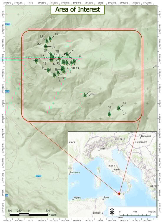
Figure 1.
Natural distribution area of Abes nebrodensis (Madonie Regional Park, Sicily, Italy). The relative tree ID is also shown for each tree. The red dot in the general map (lower-right corner) represents the study site.
2.3. Climatological and Meteorological Data
2.3.1. ERA5-Land Climatological Dataset
An important part of this research was the analysis of key climatological variables over a long-term period (spanning 75 years, from 1950 to 2024), complemented by locally observed meteorological variables. The long-term climatological analysis was conducted using the ERA5-Land climatological dataset, distributed by the European Center for Medium-Range Weather Forecasts (ECMWF). The dataset provides hourly estimates, from 1950 to nearly the present, of key climatic variables, including precipitation and temperature, at a spatial resolution of approximately 9 km [21]. The analysis was conducted on the pixel in which the study area is located (pixel center coordinates: 13°59′54″ E 37°47′48″ N). Temperature and precipitation data were resampled from hourly to daily frequency, then aggregated to monthly and annual time steps, to derive time series for several variables: average temperature (TAAT), average coldest-month temperature (TACM), average hottest-month temperature (THAT), average absolute minimum temperature (TAAMT), and monthly and yearly cumulative precipitation (PM and PY, respectively). The Standardized Precipitation Evapotranspiration Index (SPEI) was employed in this study to quantitatively evaluate the spatio-temporal variability of aridity conditions. The potential evapotranspiration (PET) was computed using the Penman–Monteith equation, which is widely recognized for its accuracy in representing evapotranspiration processes [22]. The SPEI values were computed at a 12-month temporal scale, facilitating the characterization of long-term aridity patterns within the study area.
2.3.2. Observed Weather Dataset
Meteorological data were acquired from the Cesarò–Monte Soro weather station, located in the nearby Nebrodi Park, about 60 km from the area of interest (1847 m elevation a.s.l.; latitude: 37°55′51″; longitude: 14°41′36″). These data are managed and distributed by the Sicilian Agro-Meteorological Information Service (SIAS) of Regione Siciliana [23] and cover the period from 2002 to 2024.
The daily frequencies of the following meteorological variables were resampled to monthly (Mt), annual (Y), and seasonal (Se) frequencies: average temperature (TmO; o = observed), maximum temperature (TmaxO), minimum temperature (TminO), precipitation (PO), relative humidity of air (Rh), potential evapotranspiration (PET), mean wind speed (SWO), maximum wind speed (SWmO), and prevailing wind direction (DirWO). In addition, the number of days with no precipitation (Po < 2 mm), the maximum length of periods with no precipitation, the number of days with maximum temperature To > 30 °C, the number of days with heat waves (Hwday; a heat wave is defined as a period at least 6 continuous days with TmaxO > 32), and the number of heat waves (NHw) were calculated for each year. The variables related to wind direction and speed were used to derive wind-rose diagrams, both for daily values and for those resampled to a monthly time step. Wind-rose diagrams were also produced using daily maximum values, selecting only values above 20 m s−1.
All variables belonging to this dataset underwent a cleaning process, as some had inconsistent or null values. The cleaning phase involved the correction of inconsistent values where possible (e.g., the presence of superscripts before or after a numeric value). Unfortunately, after cleaning, only about 10% of the dataset remained (Figure S1).
The data related to temperature and precipitation were also used to generate the Walter–Lieth diagrams.
2.4. Surveyed Area and Data Acquisition
The absolute position of trees was recorded using a Trimble Mobile Mapper 50 Global Navigation Satellite System (GNSS). The dendrometric parameters acquired for all trees were the diameter of the trunk at breast height (DBH), the crown projection in the north–south (N–S) and east–west (E–W) directions, and the trunk height. Other parameters acquired were the lateral surface (L m−2), elevation (m a.s.l.), position, and relationship with neighboring trees. In addition, all trees were grouped into three different health classes based on a damage index, which depended on the frequency (I) of reddened and blighted twigs per unit of crown surface (m2) (Table 1). The scheme reported by Frascella et al. [9] was modified, and the resulting three health classes were asymptomatic (I ≤ 0.10), symptomatic (I > 1.00), and medium (0.10 < I ≤ 1.00).

Table 1.
Dendrometric and health (based on symptoms) parameters of the 30 surveyed trees. The damage index (I) was based on the number (n) of reddened and blighted twigs per unit of crown surface, defined as the lateral surface area (L) of a cone with a height equal to that of the tree trunk and a base diameter equal to the diameter of the crown at its bottom (I = n/L).
A DJI Phantom 4 Multispectral quadcopter was used for aerial imagery collection. The drone was equipped with a compact multispectral camera that can acquire different bands simultaneously: Blue (B; 450 nm ± 16 nm wavelength), Green (G; 560 nm ± 16 nm wavelength), Red (R; 650 nm ± 16 nm wavelength), red-edge (B; 730 nm ± 16 nm wavelength), and near-infrared (NIR; 840 nm ± 26 nm wavelength). The camera had a focal length of 5.74 mm and captured images at a resolution of 1600 × 1300.
The 84 ha area was covered with 12 different flights that allowed a survey of almost all trees. Seven trees were excluded from the survey (nos. 1, 2, 21, 22, 25, 30, and 31) for technical reasons. The flights were conducted over the sites on 1–2 August 2023 when the trees were experiencing higher temperatures and lower rainfall. To minimize shadows, the flights were carried out around solar noon. All aerial photos were acquired with a Ground Sample Distance (GSD) average of ≈10 cm.
The above-ground-level (AGL) value of each survey was calculated considering all inherent parameters, and it ranged from 60 m to 80 m. The dedicated DJI Terra software (Version 5.0.1) was used to plan the flights, where the user defines the area of interest, flight direction, longitudinal and lateral overlap, and Ground Sample Distance (GSD). The obtained images were aligned by matching the tie points across all adjacent images using the Structure from Motion (SfM) photogrammetry technique [24] and the Agisoft PhotoScan Professional software (Version: 1.8 build 13111, 64 bit, Agisoft LLC, St. Petersburg, Russia).
2.5. Image Processing and Extraction of Vegetation Indices (VIs)
The crown of each fir tree was digitized through on-screen photointerpretation using ArcGIS Pro software (Release 3.3, ESRI 2024). Utilizing an overlay raster extraction technique, all pixels corresponding to each tree crown were extracted from the VI images. For each VI, distribution graphs of pixel values corresponding to the three health state groups were generated. The raster extraction of VI values and the generation of PDFs were conducted using a custom script within the Conda ecosystem, employing the Python programming language (Version 3.9.21) along with the Rasterio (Version 1.4.3) [25], NumPy (Version 2.2.2) [26], and Pandas (Version 2.2.0) [27,28] libraries.
Four distinct vegetation indices (VIs) were calculated through spatial analysis operations: NDVI, Green NDVI, red-edge NDVI, and ExGreen (Table 2). The choice of these indices was driven by the fact that recent studies have pointed out that these indices are the most successful in discriminating the symptomatic status of plants [29].
Table 2.
Vegetation indices used.
To support the visual classification of crown health status, isocline plots were developed for the VIs, adopting the average VI values of each fir crown and the two spectral bands involved.
The key statistical parameters for each VI, including the mean, median, first quartile, third quartile, minimum value, maximum value, CV, and range, were calculated.
Differences among health state groups were tested using the one-way analysis of variance (ANOVA) and Tukey’s HSD post hoc test. The results are presented using box plots to facilitate comparative analysis.
2.6. Spectral Analysis
Spectral analysis was conducted on 18 trees, categorized into the three health status groups based on observed symptoms. For each tree, pixel distributions were extracted for the five acquired bands (Blue, Green, Red, red-edge, and near-infrared), from which spectral signatures were derived. Based on a direct visual classification of the health status of each tree, spectral signatures were analyzed in relation to both the tree’s health condition and its topographical position, as well as in relation to neighboring trees. Subsequently, using pixel distributions, a pairwise comparison of trees was performed to derive spectral distances by applying two well-established metrics: the Spectral Angle Mapper (SAM) [33] and the Jeffries–Matusita distance (JMD) [34].
2.7. Software and Coding
The Python programming language was used to download the ERA5-Land dataset with the CDSAPI (Climate Data Store Application Program Interface).
Special procedures were also developed in the Python language for analyzing the observed meteorological data to derive general statistics, trends, and significance, and to implement advanced procedures applied to the spectral bands and vegetation indices. The temperature and precipitation trends for the ERA5-Land data were analyzed using the non-parametric Mann–Kendall test [35].
Scientific Python libraries, such as Xarray (Version 2025.01.02) [36,37], Rasterio, Geopandas (Version 1.0.1) [38], Pandas, Scikit-Learn (Version 1.3) [39], Statsmodels (Version 0.14.4) [39], Mann–Kendall (Version 1.4.3) [35], and Scipy (Version 1.15.2) [40], were used for data raster processing, statistical analysis, and the production of tables and reports. Matplotlib (Version 3-10-1) [41] and Seaborn (Version 0.13) [42] modules were used to build infographics and plots.
3. Results
3.1. Climatological Analysis
3.1.1. Long-Term Analysis
The annual temperature anomalies derived from the ERA5-Land climatological dataset for the period 1950–2024 for the study area are reported in Figure 2. A pronounced increase of 0.018 °C per year was identified over the entire period, supported by strong statistical significance (p-value < 0.001; R2 = 0.35), indicating a warming trend. Negative anomalies occurred from approximately 1960 to 1990, peaking in the mid-1970s. Positive anomalies were recorded from 2012 on, and the warming intensified markedly from 2011 to 2024, exhibiting a rate of 0.095 °C per year with very high statistical significance (p-value < 0.001; R2 = 0.75). Analysis of the last normal climatological period (1991–2020) revealed a similarly significant warming trend, although at a lower magnitude (0.026 °C per year; p-value = 0.006; R2 = 0.27).
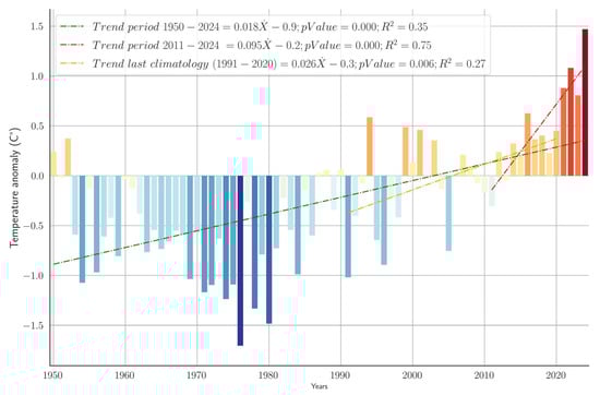
Figure 2.
Yearly average temperature anomalies. Baseline: Climatology 1991–2020. Temperature anomalies are visualized through graduated color intensities, with shades of blue indicating negative anomalies (cooler-than-average years) and shades of red depicting positive anomalies (warmer-than-average years).
The annual precipitation anomalies derived from the ERA5-Land climatological dataset for the period 1950–2020 are illustrated in Figure 3. A linear regression analysis, indicated by the dashed green line, reveals a slight positive trend (0.437 mm year−1); however, this trend is not significant (p-value = 0.592), suggesting no conclusive long-term directional change in annual precipitation. Notable periods of positive anomalies, indicating wetter-than-average conditions, are observable primarily in the early 1970s and again around 2010, with peaks exceeding 300 mm rainfall. Conversely, pronounced negative anomalies, indicative of drought conditions, occurred during the late 1950s and late 1980s, and notably intensified between 1990 and the early 2000s.
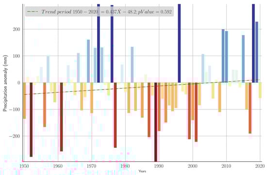
Figure 3.
Yearly average precipitation anomalies. Baseline: Climatology 1991–2020. Precipitation anomalies are visualized through graduated color intensities, with shades of blue indicating positive anomalies (wetter-than-average years) and shades of red depicting negative anomalies (drier-than-average years).
Figure 4 shows a time-series analysis of the SPEI for the period between 2010 and 2024. Positive SPEI values indicate periods of relative moisture surplus, whereas negative values correspond to drought episodes characterized by significant water deficits. A noteworthy observation is the increasing frequency and intensity of negative SPEI values in recent years (2023 and 2024).
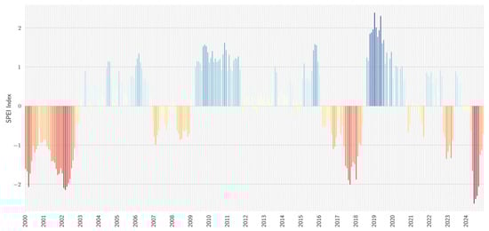
Figure 4.
Time series of SPEI from 2010 to 2024. SPEI values are visualized through graduated color intensities, with shades of blue indicating positive anomalies (humidity) and shades of red depicting negative anomalies (drought). The SPEI was implemented using the Python library “Climate indices” [43], with the period 1991–2020 as a baseline.
3.1.2. Observed Meteorological Data Analysis
The temporal evolution of the temperature and precipitation derived from the observed weather variables acquired for the Cesarò–Monte Soro station, over the observational period extending from 2000 to 2024, is reported in Figure 5. Temperature trajectories, including minimum (Tmin), maximum (Tmax), and mean (Tmean) values, are presented alongside their respective 3-year rolling means, highlighting general trends and smoothing interannual variability. The Tmax anomalies demonstrate a modest upward trajectory, indicating a warming trend, especially from 2019 on. Concurrently, yearly precipitation amounts, represented in the lower panel of Figure 5, display pronounced interannual variability without an evident long-term trend, although peaks around 2010 and again between 2015 and 2020 highlight years of notably increased rainfall. No clear relationship emerged between the temperature trends and precipitation.
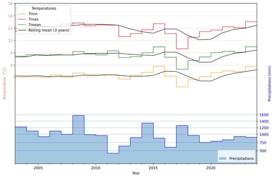
Figure 5.
Temporal evolution of temperature and precipitation derived from the observed weather variables acquired from the Cesarò–Monte Soro station.
The temporal trajectories of the yearly average potential evapotranspiration (PET, depicted in red) and relative humidity (Rh, depicted in blue), spanning the years from 2002 to 2022, were also considered (Figure 6). PET exhibited interannual variability without a distinct long-term trend, although the fluctuations indicated years of elevated evaporative demand, notably around the periods of 2010 and post-2015. Conversely, the Rh demonstrated a moderate upward trend until around 2017, after which a declining tendency was observed, suggesting shifts in atmospheric moisture conditions over the study interval. An inverse association was observed between the PET and Rh, particularly evident during periods of increased evaporative demand coinciding with decreased humidity.
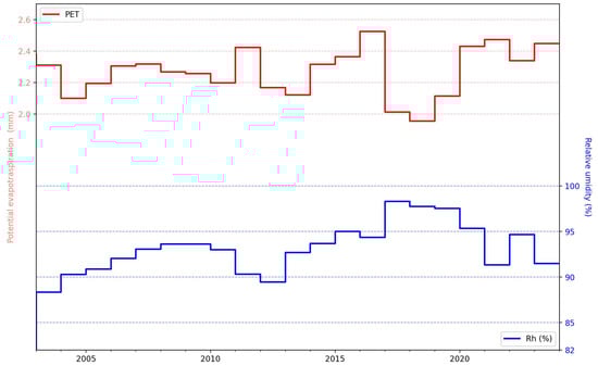
Figure 6.
Time series of PET and relative humidity derived from the observed data.
Walter–Lieth climatic diagrams [44] were derived from the Cesarò–Monte Soro’s meteorological dataset, spanning from 2002 to 2024 (Figure 7). The long-term diagram (panel a) revealed an average annual temperature of 7.6 °C and a cumulative annual precipitation of 968 mm. A pronounced seasonality is evident, characterized by a distinct humid period extending from October through April, contrasted with a drier period spanning the summer months from June to August. The highest monthly temperature averages occurred in August, peaking at approximately 22.1 °C, whereas the absolute minimum average monthly temperature of −3.4 °C was recorded in winter, primarily in January and February. The monthly precipitation demonstrated significant variability, with peak values observed in the late autumn and winter months, exceeding 100 mm rainfall per month, while notably declining to a minimum during summer, indicating a clear Mediterranean montane climate pattern. The potential occurrence of frost events was noted from December to February, signifying seasonal thermal constraints typical of high-altitude Mediterranean environments.
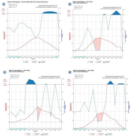
Figure 7.
Walter–Lieth climatic diagrams derived from observed data (Cesarò–Monte Soro station): (a) Long-term diagram. (b–d) Individual yearly diagrams. A dry period is defined as when monthly precipitation (in mm) is less than twice the average monthly temperature (in °C), shown with red-hatched shading. A wet (or humid) period is defined as when the monthly precipitation is equal to or greater than twice the average monthly temperature, indicated with solid blue shading.
Conversely, the diagrams representing 2022, 2023, and 2024 (panels b–d) revealed intensified drought conditions during the summer months. Among these, the year 2022 (panel b) exhibited the most severe drought stress, characterized by an extended dry period in June–July, exacerbated by higher temperatures and substantially reduced precipitation compared to the long-term average. Pronounced drought events also occurred in mid-summer in 2023 and 2024 (panels c and d), albeit somewhat less severe.
A temporal analysis of dry-day occurrences and their continuity over the period from 2003 to 2024 was conducted (Figure 8). The histograms in (a) illustrate the annual frequency of dry days, defined as days with precipitation below 1 mm. Consistent interannual variability was observed, with the highest number of dry days recorded in 2017 (209 days) and the lowest in 2009 (151 days). No clear trend was evident from the time series, although periods of relatively higher dryness, such as 2004–2007 and 2019–2021, were noticeable. Subfigure (b) depicts the maximum annual duration of continuous dry spells, revealing substantial variability among years. Notably, the longest dry spell occurred in 2012 (51 days); conversely, the shortest maximum dry spell was recorded in 2015 (16 days).
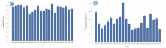
Figure 8.
Annual analysis of dry-day frequency and maximum dry-spell duration for the period 2003–2024. (a) Total number of dry days per year, defined as days with precipitation amounts lower than 2 mm. (b) Annual maximum duration of consecutive dry days (dry spells), applying the same precipitation threshold (<2 mm/day).
The results of an analysis of climatic variability by examining minimum temperature extremes during April and May, spanning from 2003 to 2024, are reported in Figure 9. Subfigure (a) illustrates the annual frequency of late frost days, defined as days during April and May when the minimum daily temperature (Tmin) was less than or equal to 0 °C. The data revealed substantial interannual fluctuations, with particularly high occurrences observed in 2019 (22 days) and 2023 (16 days). Conversely, several years, notably 2010, 2014, and 2016, exhibited the lowest frequency of such conditions (3 days each). Subfigure (b) displays the maximum duration of consecutive late frost days during the same months and under the same temperature threshold. Prominent, prolonged late frost spells occurred in 2019 (11 days) and 2023 (10 days), whereas shorter maximum late frost spells were recorded in 2010, 2011, 2014, and 2016 (3 days each).
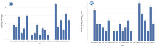
Figure 9.
(a) Number of days per year in April and May when the minimum daily temperature was less than or equal to 0 °C. (b) Maximum duration of consecutive late frost days per year during the same period (Tmin < 0).
The annual variability in temperature extremes, based on the frequency of days falling within specific percentile thresholds of minimum daily temperatures (Tmin) from 2002 to 2024, is presented in Figure 10. Figure 10a illustrates the annual number of days characterized by Tmin values equal to or below the 10th percentile, indicating episodes of notably low temperatures. The data obtained demonstrated marked interannual variability, with distinct peaks observed in 2005 (48 days), 2006 (45 days), and 2019 (47 days), whereas notably fewer occurrences were recorded in 2002 (12 days) and 2017 (13 days). Figure 10b depicts the annual frequency of days with Tmax equal to or exceeding the 90th percentile, representing episodes of high maximum temperatures. Prominent peaks occurred in 2008 (49 days) and 2023 (48 days), contrasted sharply with low occurrences in 2002 (9 days) and 2018 (6 days).
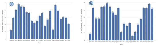
Figure 10.
(a) Number of days per year when the minimum daily air temperature (Tmin) was below the 10th percentile threshold. (b) Number of days per year when the maximum daily air temperature (Tmax) exceeded the 90th percentile threshold. The time series span from 2002 to 2024.
An analysis of the cumulative summer precipitation totals and the extreme intra-period temperature range from 2003 to 2024 also revealed the variability of climatic conditions, as reported in Figure 11. Figure 11a depicts the cumulative summer precipitation totals, highlighting pronounced interannual fluctuations, with a prominent peak in precipitation during 2018 (521 mm), contrasting notably with particularly dry summers in 2009 (35 mm) and 2017 (41 mm). Such variability indicates alternating wet and dry episodes, underscoring the non-uniform nature of precipitation regimes during the study period. Figure 11b presents the extreme intra-period temperature range, calculated as the difference between the highest daily maximum temperature (TXx) and the lowest daily minimum temperature (TNn) for each year. A relatively stable yet elevated variability was observed throughout the analyzed years, with the largest temperature range occurring in 2008 (44 °C) and the lowest in 2002 (27 °C).
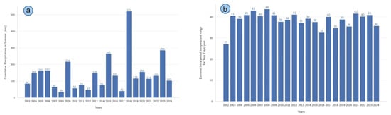
Figure 11.
(a) Cumulative summer precipitation totals (mm) per year from 2003 to 2024. (b) Annual extreme intra-period temperature range, calculated as the difference between the highest daily maximum temperature (TXx) and the lowest daily minimum temperature (TNn) recorded each summer.
Figure 12 presents wind-rose diagrams depicting the daily mean wind-speed distribution (left) and the enhanced representation of the daily maximum wind speeds (right) observed within the study area. Each concentric circle on the radial axis represents an incremental percentage of occurrence, thereby allowing a straightforward visual comparison of how often specific wind directions and speeds are recorded. Color gradations reflect discrete velocity ranges, expressed in meters per second, enabling an immediate assessment of wind intensity variability across each directional sector.
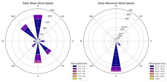
Figure 12.
Wind-rose diagrams representing the daily mean wind speed (left panel) and the daily maximum wind speed (right panel) across different wind directions.
The daily wind speed predominantly originates from the northern and southern sectors, exhibiting wind velocities generally below 10 m s−1, as highlighted by the dominance of lower velocity classes. Conversely, the daily maximum wind speeds illustrate a more distinct and narrower distribution, characterized by an increased frequency of higher velocity categories (>15 m s−1), particularly evident from the southern directions (60% of cases).
The results of monthly resampling of wind data, illustrating both the dominant wind directions and the frequency distribution of wind speeds, are shown in Figure 13. The mode, or most frequently observed sector, has been determined for every monthly interval, revealing a pronounced tendency for winds to originate from the northern and southern quadrants. The left panel depicts the monthly mean wind speeds, indicating prevailing winds predominantly originating from the northern and northwestern sectors, mostly within lower speed ranges (<5 m s−1). In comparison, the right panel illustrates the monthly maximum wind speeds, highlighting occurrences of significantly higher velocities, particularly from the northern and southern directions. Maximum velocities frequently exceed 20 m s−1, with occasional events surpassing 40 m s−1.
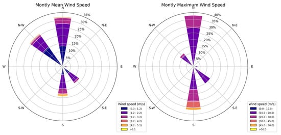
Figure 13.
Wind-rose diagrams illustrating the monthly mean wind speed (left panel) and the monthly maximum wind speed (right panel) across different wind directions.
Monthly maximum wind-speed values recorded in the study area over the observational period, spanning from 2002 to 2024, were also considered (Figure 14). The temporal pattern displays notable interannual variability, characterized by frequent fluctuations between moderate (approximately 10–20 m s−1) and elevated wind-speed events, reaching values exceeding 40 m s−1. A prominent peak, approaching 50 m s−1, is clearly discernible around the year 2013, suggesting a significant extreme wind event during that period. Furthermore, the frequency and magnitude of wind-speed maxima appear to intensify toward the latter part of the record, particularly after 2019, indicating a potential shift toward conditions favoring higher wind intensity.
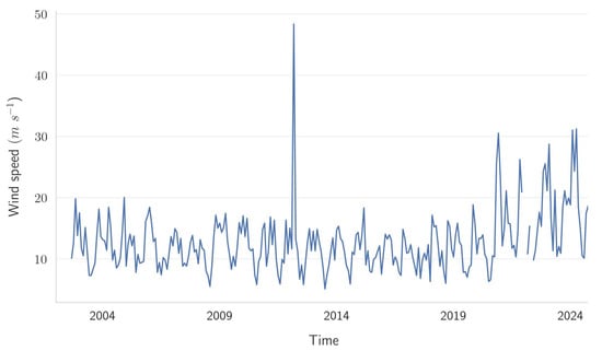
Figure 14.
Time series of monthly maximum wind-speed values.
Such evidence underscores the relevance of analyzing extremes in wind speed to effectively characterize disturbances and support informed decision-making related to infrastructure resilience, risk management, and adaptation strategies within the investigated site.
The combined analysis of Figure 13 and Figure 14 provides valuable insights into wind behavior within the investigated area by illustrating both the temporal variability and directional prevalence of monthly maximum wind speeds. Figure 14 highlights notable temporal variability and an evident peak in the wind speed around 2013, suggesting a significant extreme event. Complementarily, Figure 13 identifies the predominant directions associated with these maximum wind-speed episodes, clearly emphasizing a marked influence of the northern and southern sectors.
3.2. Spectral Analysis Outcomes
In Figure 15, the spectral signatures of 18 fir trees are reported, categorized by observed crown symptoms (panel a) and location site (panel b). Notably, the near-infrared (NIR) and red-edge bands demonstrated superior sensitivity in discriminating tree health conditions compared to the visible spectral bands (Blue, Green, and Red).
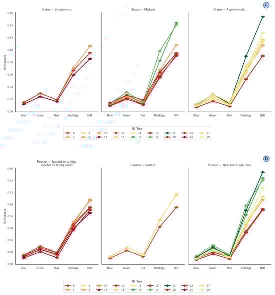
Figure 15.
Spectral signatures of fir trees classified by symptom status (a) and spatial positioning (b). Spectral bands (Blue, Green, Red, red-edge, and near-infrared (NIR)) are reported on the x-axis, and reflectance values are indicated on the y-axis. Error bars associated with each data point represent the 95% confidence interval.
The first set of spectral profiles clearly differentiates trees by their physiological condition, revealing significant spectral variability, primarily in the near-infrared (NIR) and red-edge regions. Trees classified as symptomatic demonstrated notably lower NIR reflectance, indicating reduced vegetative vigor compared to asymptomatic trees, which exhibited substantially higher reflectance values. The intermediate group (medium symptom severity) occupied a spectral range between symptomatic and asymptomatic trees, suggesting a gradation in physiological conditions detectable through spectral analysis. The second set highlights the spectral variations associated with tree location. Fir trees located near beech or oak groves displayed higher reflectance values, particularly in the NIR spectrum, compared to isolated trees. In contrast, isolated trees, particularly those situated on exposed ridges and subjected to strong winds, exhibited diminished reflectance, indicative of greater physiological stress.
The Jeffries–Matusita (JM—panel a) and Spectral Angle Mapper (SAM—panel b) distance metrics are displayed in Figure 16. For the JM distance, the broader color patterns reveal that certain “symptomatic” versus “medium” pairings exhibited relatively elevated JM distances, suggesting distinct reflectance characteristics in these classes. Conversely, some “symptomatic” trees are clustered in intermediate ranges, indicating a moderate separation from both “medium” and “asymptomatic” classes.
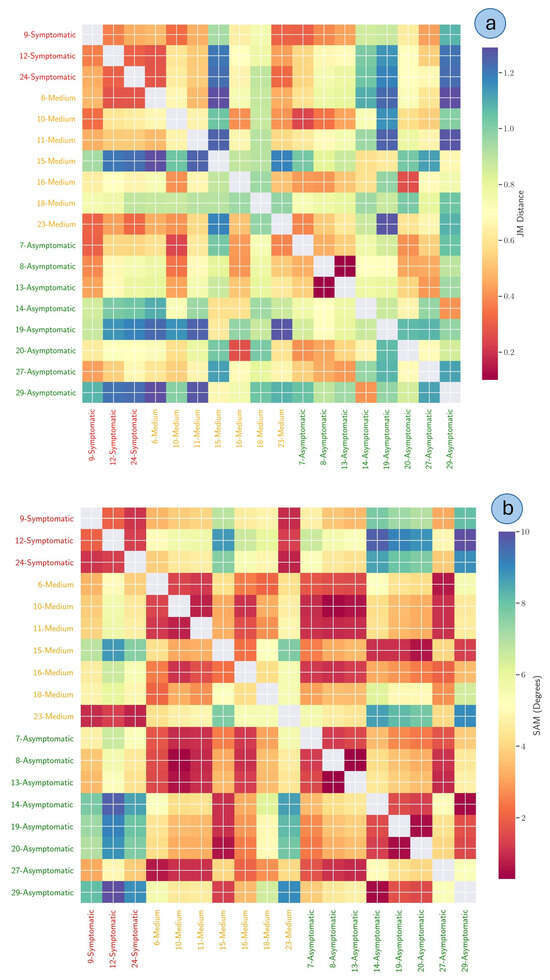
Figure 16.
Jeffries–Matusita (JM—panel (a)) and Spectral Angle Mapper (SAM—panel (b)) distance metrics visualized as heatmaps, both representing pairwise comparisons of tree crowns grouped by individual identifier and physiological status. The rows and columns correspond to the classes (e.g., “symptomatic”, “medium,” and “asymptomatic” crowns), and the color scale depicts increasing spectral separability from warmer hues (low JM or SAM distance) to cooler hues (high JM or SAM distance). Notably, the zeros on the main diagonal reflect each class’s comparison with itself; thus, they are excluded from the overall interpretation.
Upon analyzing the SAM distance (panel b), some “asymptomatic” versus “symptomatic” pairings exhibited notably large distances, suggesting pronounced reflectance divergence. Conversely, some “medium” classes are clustered at intermediate color levels, indicating moderate separation from both “asymptomatic” and “symptomatic” classes. The patchwork pattern in the heatmap further reveals potential subtleties, as certain trees with the same health status can display non-negligible spectral variation, underscoring the SAM method’s sensitivity to subtle differences in reflectance profiles.
3.3. Analysis of VIs
Table 3 presents the descriptive statistics of the Normalized Difference Vegetation Index (NDVI) grouped by tree health status (asymptomatic, medium, and symptomatic). The asymptomatic group exhibited the highest mean NDVI (0.78, ranging from 0.75 to 0.85), with a narrow confidence interval ranging from 0.78 (CI low) to 0.79 (CI high), and a low standard deviation (0.03), indicating high consistency among sampled trees. Trees with medium symptom severity displayed a slightly lower mean NDVI of 0.78 (range 0.68–0.82), accompanied by a similarly narrow confidence interval (CI low = 0.78, CI high = 0.78) and a modestly increased standard deviation (0.11). The symptomatic group showed a lower mean NDVI value (0.67, ranging from 0.66 to 0.68), which is indicative of reduced vigor. Furthermore, this group demonstrated greater variability, as indicated by a higher standard deviation (0.08) and a wider confidence interval.
Table 3.
Descriptive statistics of the NDVI grouped by tree health status, obtained for each sampled tree based on the number of pixels captured from the multispectral images. n. pixels: number of pixels per tree crown; mean: mean NDVI for each sampled plant; sem: standard error; median: median value; min: minimum value; max: maximum value; std: standard deviation; q0.25: first quartile; q0.75: third quartile; CI low: lower confidence interval; CI high: upper confidence interval.
Table 4 summarizes the descriptive statistics of the Green Normalized Difference Vegetation Index (Green NDVI), categorized by tree health status (asymptomatic, medium, and symptomatic). The asymptomatic group exhibited the highest mean Green NDVI value (0.64), with a narrow confidence interval ranging from 0.64 (CI low) to 0.64 (CI high) and a relatively low standard deviation (0.13), reflecting limited variability within this group. Trees with medium symptom severity showed an identical mean Green NDVI (0.64) with a similarly tight confidence interval (CI low = 0.64, CI high = 0.64) but exhibited slightly less variability (standard deviation = 0.09). In contrast, the symptomatic group had the lowest mean Green NDVI (0.53), indicating diminished vegetation vigor. This group also presented a narrow confidence interval (CI low = 0.53, CI high = 0.53) and moderate variability (standard deviation = 0.07). These findings confirm a clear association between declining Green NDVI values and increased severity of symptoms, supporting the utility of the Green NDVI as an effective indicator of tree health condition.
Table 4.
Descriptive statistics of the Green NDVI grouped by tree health status, obtained for each sampled tree based on the number of pixels captured from multispectral images. n. pixels: number of pixels per tree crown; mean NDVI for each sampled plant; sem: standard error; median: median value; min: minimum value; max: maximum value; std: standard deviation; q0.25: first quartile; q0.75: third quartile; CI low: lower confidence interval; CI high: upper confidence interval.
Table 5 provides the descriptive statistics of the Excess Green (ExGreen) vegetation index, categorized by tree health status (asymptomatic, medium, and symptomatic). The mean ExGreen values across all health statuses remained uniformly low, each exhibiting a mean of 0.02 for asymptomatic trees and trees with medium symptom severity and a slightly lower mean of 0.01 for symptomatic trees. The confidence intervals were narrow and consistent within each category (CI low = 0.02, CI high = 0.02 for asymptomatic trees and trees with medium symptom severity; CI low = 0.01, CI high = 0.01 for symptomatic trees). Standard deviations were also consistently low across groups (asymptomatic: std = 0.009; medium: std = 0.010; symptomatic: std = 0.012), indicating minimal variability in ExGreen values within each health status. Despite the subtle numerical differences observed, symptomatic trees consistently presented slightly lower ExGreen values, suggesting this index, though displaying minimal variation, may still possess limited utility as a supportive indicator of reduced vegetation health.
Table 5.
Descriptive statistics of the ExGreen index grouped by tree health status, obtained for each sampled tree based on the number of pixels captured from the multispectral images. n. pixels: number of pixels per tree crown; mean: mean NDVI for each sampled plant; sem: standard error; median: median value; min: minimum value; max: maximum value; std: standard deviation; q0.25: first quartile; q0.75: third quartile; CI low: lower confidence interval; CI high: upper confidence interval.
Table 6 presents the statistical metrics of the red-edge Normalized Difference Vegetation Index (red-edge NDVI), categorized by tree health status (asymptomatic, medium, and symptomatic). Asymptomatic trees demonstrated the highest mean red-edge NDVI (0.25), accompanied by a narrow confidence interval (CI low = 0.25, CI high = 0.25) and moderate variability, indicated by a standard deviation of 0.07. Trees with medium symptom severity exhibited a slightly lower mean red-edge NDVI (0.23), similarly characterized by a concise confidence interval ranging from 0.23 (CI low) to 0.23 (CI high), yet exhibited higher variability (std = 0.07) akin to the asymptomatic group. Symptomatic trees recorded the lowest mean red-edge NDVI value (0.18), with a correspondingly narrow confidence interval (CI low = 0.18, CI high = 0.18) and slightly higher variability (std = 0.09). These observations suggest decreasing red-edge NDVI values associated with reducing tree health, supporting the use of the red-edge NDVI as a discriminator of vegetation stress across health conditions.
Table 6.
Descriptive statistics of the red-edge NDVI grouped by tree health status, obtained for each sampled tree based on the number of pixels captured from the multispectral images. n. pixels: number of pixels per tree crown; mean: mean NDVI for each sampled plant; sem: standard error; median: median value; min: minimum value; max: maximum value; std: standard deviation; q0.25: first quartile; q0.75: third quartile; CI low: lower confidence interval; CI high: upper confidence interval.
Violin plots illustrating the distribution of VI values (NDVI, Green NDVI, red-edge NDVI, and ExGreen) across trees categorized by symptom group (asymptomatic, medium, symptomatic) are presented in Figure 17. The NDVI and Green NDVI clearly discriminated between groups, exhibiting the highest median values for asymptomatic trees, intermediate values for trees with medium symptom severity, and the lowest for symptomatic trees, with statistically significant differences confirmed by Tukey’s test (indicated by different letters: a, b, c). In contrast, the red-edge NDVI showed a similar but less pronounced trend, yet it still significantly distinguished among all three groups. The ExGreen index, however, demonstrated considerable overlap between groups and minimal variation, indicating limited efficacy for symptom discrimination, despite the statistical significance indicated.
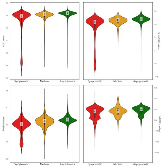
Figure 17.
Violin plots showing the distribution of VI values grouped by symptom category. Asymptomatic: no symptoms observed; Medium: trees with 0.11 < I < 1.00, i.e., fewer than one symptomatic twig per square meter of crown surface; Symptomatic: trees with I > 1.00, i.e., more than one symptomatic twig per square meter of crown surface. The letters above the violin plots indicate statistically significant groupings based on a post hoc analysis, highlighting differences among groups.
The spatial distribution of the sampled trees based on the mean NIR and red-edge reflectance is reported in the NDVI isocline plots (Figure 18). Trees categorized as asymptomatic (green markers) predominantly occupy positions in the higher NDVI isoclines (≥0.80), reflecting greater vegetation health and vigor. In contrast, trees with medium symptom severity (dark beige markers) primarily fall within intermediate NDVI ranges (0.70–0.80), indicating moderate vegetation stress. Trees categorized as symptomatic (red markers) consistently occupy positions in the lower NDVI isoclines (≤0.70), demonstrating significantly reduced vegetation conditions. This distribution underscores a clear gradient in tree health status, with asymptomatic trees consistently exhibiting higher NDVI values compared to symptomatic trees and trees with medium symptom severity. These results reinforce the applicability of the NDVI as an effective remote sensing indicator for distinguishing varying degrees of tree health conditions.
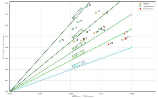
Figure 18.
NDVI isocline plot. Each A. nebrodensis tree is positioned in the plot based on the mean NIR and red-edge reflectance. Green markers: healthy trees; dark beige markers: trees with medium symptom severity (0.11 < I > 1.00), i.e., fewer than one symptom; red cross marker: symptomatic trees.
Figure 19 illustrates the Green NDVI isocline plot depicting the distribution of sampled trees based on the mean NIR and red-edge reflectance values. Trees classified as asymptomatic (green markers) predominantly cluster within higher Green NDVI isoclines (≥0.70), reflecting robust vegetation health. Trees with medium symptom severity (dark beige markers) primarily occupy intermediate positions, ranging between Green NDVI values of 0.60 and 0.70, indicating moderate vegetative stress. Conversely, trees identified as symptomatic (red markers) consistently appear at lower Green NDVI isoclines (≤0.60), suggesting compromised vegetative conditions. The clear positional separation among the tree health groups reinforces the effectiveness of the Green NDVI as an indicator capable of discriminating between different degrees of vegetative health in sampled tree populations.
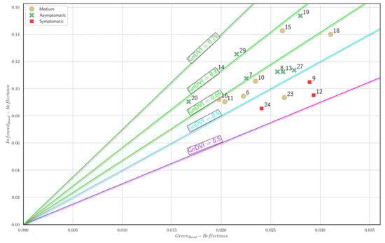
Figure 19.
Green NDVI isocline plot. Each A. nebrodensis tree is positioned in the plot based on the mean NIR and red-edge reflectance. Green markers: asymptomatic trees; dark beige markers: trees with medium symptom severity; red cross marker: symptomatic trees.
Figure 20 presents the isocline plot for the red-edge Normalized Difference Vegetation Index (red-edge NDVI), illustrating tree positions based on the mean NIR and red-edge reflectance. Trees classified as asymptomatic (green markers) are predominantly located along higher red-edge NDVI isoclines (≥0.25), highlighting superior vegetative health relative to the other groups. Trees with medium symptom severity (dark beige markers) are mainly distributed within intermediate red-edge NDVI values (approximately 0.15–0.25), signifying moderate stress. In contrast, symptomatic trees (red markers) consistently occupy lower positions on the plot (red-edge NDVI ≤ 0.15), indicating reduced vegetation vigor and heightened stress levels. The clear separation between tree health categories demonstrates that the red-edge NDVI effectively differentiates between varying degrees of vegetative health and could serve as a reliable indicator in vegetation monitoring studies.
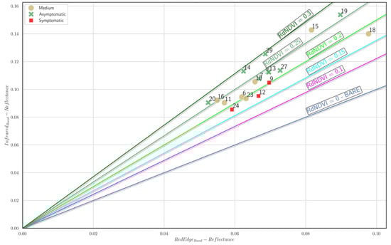
Figure 20.
Red-edge NDVI isocline plot. Each A. nebrodensis tree is positioned in the plot based on the mean infrared and red-edge reflectance. Green markers: asymptomatic trees; dark beige markers: trees with medium symptom severity; red cross marker: symptomatic trees.
The comparative analysis of the isocline plots for the vegetation indices (NDVI, Green NDVI, and red-edge NDVI) presented in Figure 18, Figure 19 and Figure 20 demonstrates distinct capabilities in discriminating between tree health statuses (asymptomatic, medium, and symptomatic). The NDVI (Figure 18) showed the clearest differentiation among health groups, effectively separating asymptomatic trees at higher isoclines (>0.80) from symptomatic trees (<0.70). The Green NDVI (Figure 19) also provided robust separation, with asymptomatic trees predominantly occupying isoclines ≥0.70 and symptomatic trees clearly clustering below the 0.60 threshold. However, the red-edge NDVI (Figure 20) exhibited good discriminative power among health conditions, distinctly positioning the asymptomatic, medium, and symptomatic categories along well-defined gradients (≥0.25, 0.15–0.25, and ≤0.15, respectively). Among the indices analyzed, the red-edge NDVI and NDVI emerged as the superior discriminators of tree health, providing more precise separation between symptom categories, thus indicating their suitability as effective remote sensing indicators for early detection and monitoring of tree stress conditions.
4. Discussion
The present research is aimed at assisting the ongoing effort to monitor and conserve Abies nebrodensis, a critically endangered Mediterranean fir endemic to Sicily. An integrated methodological approach that combines UAV-based remote sensing, analysis of climatological and observed meteorological data, and traditional phytosanitary inspections has been evaluated. Such an interdisciplinary approach has been advocated by recent studies as essential for the comprehensive monitoring of endangered species and their habitats [2].
The study findings align with the existing literature, underscoring the vulnerability of A. nebrodensis due to its limited population size and fragmented distribution. Specifically, remnants are confined to the upper slopes and ridges of the Madonie Regional Park (Figure 1), an environment that exposes this species to various stressors, including climatic extremes [45,46].
In general, the inclusion of long-term climatological analyses using the ERA5-Land dataset provides essential context for the observed trends in plant health. Climate change impacts, especially the rise in extreme heat events, increased drought severity, and altered phenology, significantly affect Mediterranean forest ecosystems [15,16]. The current findings generally indicate a clear relationship between climatic conditions (particularly temperature, precipitation, and wind gust patterns) and the physiological status of trees, as evidenced by the analysis of spectral vegetation indices [47]. These observations complement recent reports of increased heatwave frequency and severity in Italy [12]. Consequently, addressing climate-driven risks through integrated monitoring becomes paramount for the sustainable management of A. nebrodensis and other similarly vulnerable species, such as other Mediterranean firs (Abies pinsapo, A. equi-trojani, A. marocana, and A. numidica), Zelkova sicula, Cedrus brevifolia, and Tetraclinis articulata populations in Malta and Spain, among others. The observed climatic trend can markedly influence the health and resilience of the A. nebrodensis population, as persistent drought stress reduces soil moisture availability, adversely affecting essential physiological processes such as photosynthesis, growth, and nutrient uptake.
Although the historical analysis of the climatological dataset conducted in this study did not reveal dramatic changes, it did indicate the occurrence of positive temperature anomalies beginning in 2011. While precipitation anomalies indicated no clear trend, the SPEI suggested a progressive shift toward more severe, prolonged, and recurrent drought conditions in recent years.
The analysis of observed meteorological data also evidenced a gradual increase in mean and minimum temperature anomalies, suggesting an overall warming tendency, particularly since 2020.
Regarding water availability, the Walter–Lieth climatic diagrams for the years 2022, 2023, and 2024 also indicated a recent worsening in drought conditions, underscoring a trend toward increased climatic stress at this location, potentially associated with broader regional climate change. Such findings emphasize the importance of examining climatic variability at shorter temporal scales to accurately identify and respond to emerging drought trends and their ecological implications. The duration of dry spells also showed substantial variability between years without revealing any particular trend. This underscores the interannual variability of drought conditions, emphasizing the complex dynamics of dry period occurrences and continuity within the analyzed timeframe.
Nevertheless, the inverse relation displayed by PET and Rh (as shown in Figure 5) highlights the intricate interplay between evaporative processes and atmospheric moisture availability. These findings underscore the importance of examining concurrent variations in PET and Rh to better understand climate-driven changes affecting regional water-balance dynamics and how these changes may affect the health status of Sicilian fir.
Another stress factor for A. nebrodensis in its habitat is late frosts. The results concerning the occurrence and duration of minimum temperature extremes in April and May underscore a pronounced interannual variability in spring-season climate conditions, emphasizing the occurrence of late frost events, which may impact tree physiology and contribute to crown disorders. Significant variability was also observed in the occurrence of extreme temperatures, particularly in both low and high Tmin values. Notably, since 2017, there has been a consistent increase in the number of days each year when the maximum temperature exceeded the 90th percentile threshold. While no clear linear correlation between cumulative precipitation and temperature extremes is evident from the graphs in Figure 11, the data highlight significant climatic variability, reflecting complex interactions that potentially influence ecosystem dynamics during summer periods.
The analysis of wind speed and direction, reported in the wind-rose diagrams (Figure 12 and Figure 13), revealed substantial differences between average wind conditions and peak wind events, underscoring the importance of considering both routine and extreme wind occurrences separately. Such differentiation is essential for comprehensive climate risk assessments, the protection of infrastructure, and the development of environmental management strategies. The combined analysis of the predominant directions associated with maximum wind-speed episodes suggests a directional persistence of extreme winds, which can inform targeted assessments of resilience, guide environmental management practices, and support future planning strategies aimed at mitigating wind-related risks at the site. Exposure to strong winds is indeed one of the environmental factors with the greatest impact on the A. nebrodensis population, particularly for trees located on ridges or in the middle of ravines and screes.
Notably, the enhanced scaling for daily maximum wind speeds clearly highlights episodes of stronger winds exceeding 20 m s−1, indicating occasional intense wind events that may be relevant for local climatic studies and hazard assessments. The analysis revealed that winds predominantly originate from the north quadrant (commonly referred to as Tramontana) and the south quadrant (Scirocco), with higher frequencies observed in these two sectors. This pattern reflects the influence of large-scale circulation mechanisms that facilitate air mass movement along the meridional axis, reinforcing the observed prevalence of northerly and southerly flows. These results offer valuable insights into local wind dynamics and emphasize the importance of distinguishing between average conditions and peak events when assessing wind-related phenomena.
Assessing the impact of climate change and extreme events is a challenging task, especially for species inhabiting extreme environments. In the context of sustainable forest management, the use of vegetation spectroscopy to assess forest disturbances has gained increasing importance in recent years [29,48].
Our findings demonstrate that spectral profiles can effectively discriminate A. nebrodensis trees based on both the frequency of crown disorders (symptoms) and their exposure to different microclimatic and soil conditions, e.g., isolated trees on ridges versus those growing within or close to broadleaf groves. The spectral profiles effectively captured a gradation of physiological conditions related to tree location within the habitat. The data indicate the presence of trees that, despite being asymptomatic, showed reduced reflectance in the NIR, as well as trees in the ‘medium’ symptom class that display relatively high NIR reflectance. Furthermore, pairwise comparisons of tree crowns using the JM and SAM distance metrics (Figure 16) revealed that trees in the intermediate symptom category (medium) show relatively large distances from both symptomatic and asymptomatic trees. In other cases, pairings between trees of different symptom categories showed only moderate separation.
This spatial clustering of color blocks highlights how the JM metric effectively captures differences arising from both spectral mean and covariance properties. The resulting insights can support further analyses, such as identifying specific tree crowns or physiological conditions that exhibit marked spectral divergence and can potentially guide targeted interventions or monitoring strategies in precision forestry and related remote sensing applications. Overall, the SAM metric provides a robust measure of pixel-level spectral similarity, facilitating nuanced insights into variation across tree crowns with different physiological conditions.
An interesting finding of this work is that trees growing near or within broadleaf groves showed better overall health than isolated trees growing on rocky soils (Figure 15). This is mainly due to the thicker and more fertile soil, as well as the protection from wind and other external agents provided by the broadleaf trees. Spectral analysis clearly showed that the trees located along screes and ridges, characterized by poor soil conditions and greater exposure to strong winds, exhibited poorer health and physiological status, as also reflected by lower VI values. Safeguard strategies should focus primarily on these trees (nos. 9, 12, 23, and 24).
All the VIs used in this research proved to be useful tools for assessing the health status of A. nebrodensis trees, showing substantial correspondence with the classification based on visual observation of crown symptoms (in terms of the frequency of blighted twigs per unit of crown surface). Statistical inference analyses conducted on all indices for the three symptom classes proved to be statistically significant at the 0.05 confidence level. Among the VIs evaluated, the NIR and red-edge spectral bands were the most effective for assessing A. nebrodensis tree health and emphasized the ecological advantage provided by proximity to broadleaf groves, reflecting favorable microenvironmental conditions likely resulting from improved pedological characteristics and protection from environmental stress.
A clear gradient in the NDVI and Green NDVI values corresponded to the groups of trees defined by the frequency of observed symptoms, with declining values of both indices correlating with an increase in crown symptoms. Overall, the NDVI and Green NDVI emerged as the most effective indices for clearly differentiating tree health conditions, highlighting their utility in accurately assessing vegetation stress, according to [49].
Based on the NDVI and Green NDVI isocline plots (Figure 18 and Figure 19), some trees classified as ‘asymptomatic’ fall in the intermediate ranges of both VIs. These trees (e.g., nos. 7, 8, and 13) may exhibit physiological conditions that do not correspond to the frequency of symptoms observed on the crowns. These trees should receive particular attention in monitoring activities, as their physiological state may be worse than their visual appearance suggests. This finding indicates that spectral analyses can provide additional information beyond simple visual inspections, making them a useful complement to the monitoring of A. nebrodensis.
Although recent analysis of the fungal community associated with A. nebrodensis disorders has shown the involvement of saprophytic and endophytic fungi, excluding aggressive pathogens [9], continued and increasing climatic stress could promote disease outbreaks due to pathogens. Future studies should focus on these interactions, modeling pest and pathogen dynamics in relation to the climatic and vegetative indices identified through remote sensing techniques. Such investigations would enhance predictive capabilities for pathogen outbreaks and may assist in targeted phytosanitary interventions.
Regarding conservation methods, both Benelli et al. [46] and Frascella et al. [45] emphasize the need for a combined ex situ and in situ conservation strategy, including the establishment of seedbanks and cryobanks, to safeguard genetic diversity. This research complements those recommendations by demonstrating how advanced monitoring technologies like UAV-based multispectral imaging can support in situ management actions, allowing conservationists to promptly identify and mitigate health threats. Combining these strategies offers a powerful framework for long-term preservation efforts.
In terms of disagreements or gaps, it is noteworthy that this research primarily addresses contemporary factors impacting tree health and does not deeply engage with broader ecological processes and interactions at the ecosystem level, such as species competition, invasive species dynamics, and broader landscape-level ecological changes. A recent review of tree growth processes, crises, and management strategies [50] highlights the importance of adopting holistic, ecosystem-level perspectives, suggesting that future research could benefit from incorporating these broader ecological factors. This integration would further improve management recommendations and help ensure the resilience and sustainability of ecosystems hosting endangered species like A. nebrodensis.
Regarding the remote sensing monitoring process, which involved only a single survey with a multispectral camera, it is advisable that future monitoring efforts include at least annual surveys using a wider range of sensors (e.g., hyperspectral sensors) to obtain more detailed spectral data for analysis and interpretation.
In fact, this study has shown that the analysis of five spectral signatures and the appropriate combination of spectral bands to derive vegetation indices allows discrimination of plant health status, and the availability of significantly more bands can further enhance this detection. Future explorations should therefore also focus on acquiring hyperspectral imagery to perform an in-depth spectral analysis using a significantly higher number of spectral bands. Integrating hyperspectral data into the existing monitoring framework would provide a more comprehensive understanding of the health status of Abies nebrodensis, potentially improving conservation strategies and enabling more effective, targeted interventions.
5. Conclusions
This study expands the existing knowledge regarding the critical conservation status of Abies nebrodensis, highlighting the efficacy of integrated monitoring techniques that combine UAV-based remote sensing, climatological data analysis, and traditional phytosanitary inspections. The observed correlation between VIs derived from multispectral images and the physiological condition of trees underscores the potential of remote sensing and machine learning as powerful tools for proactive conservation strategies. Addressing the identified threats, especially climate-driven stresses that exacerbate the vulnerability of this species, requires ongoing multidisciplinary research and targeted conservation actions. Future efforts should prioritize expanded spatial and temporal monitoring, incorporate broader ecological interactions, and develop advanced predictive models to enhance the resilience and sustainability of the Sicilian fir population and similarly threatened species.
Moreover, while this study relies on the integration of dense spectral and environmental data, it is important to consider the scalability of such approaches. In sparse and fragmented populations like A. nebrodensis, individual-based monitoring remains critical. However, to extend applicability to larger or less accessible regions, emerging smart sensing paradigms such as compressive sensing [51,52,53] may offer new opportunities to reduce data requirements without sacrificing precision. These approaches, based on signal sparsity and reconstruction algorithms, could enhance the operational feasibility of large-scale conservation monitoring. Although our integrative method provides high spatial resolution and strong correlation between spectral indices and tree health, its extension to larger forest areas or denser populations may be limited by operational costs and data volume. Future developments could incorporate smart sensing techniques such as compressive sensing to optimize data acquisition, allowing adaptive monitoring of wider areas while maintaining diagnostic accuracy. This is particularly relevant for conservation scenarios where resources are limited, and scalable solutions are required to protect endangered species like A. nebrodensis.
In conclusion, this research aligns well with the current scientific literature, emphasizing the need for integrated and technologically advanced approaches to monitoring and conserving endangered tree species. Its interdisciplinary methodology offers promising tools for conservation, highlighting essential areas for ongoing research and collaboration among ecologists, climatologists, and conservationists.
Supplementary Materials
The following supporting information can be downloaded at: https://www.mdpi.com/article/10.3390/f16071200/s1, Figure S1: Consistent data time series. The figure represents the availability of valid weather-climate data. With yellow colour, for each variable (x-axis), consistent values are represented along time (y-axis), and with purple colour, null and unavailable values for the weather-climate data analyst.
Author Contributions
Conceptualization, L.A., M.C. and R.D.; methodology, L.A.; software, L.A.; validation, L.A., R.D., S.B., G.E. and G.D.R.; formal analysis, L.A., M.C. and R.D.; investigation, L.A., S.B., G.E. and R.D.; data curation, L.A. and R.D.; writing—original draft preparation, L.A., M.C., G.D.R., S.B., G.E., D.P., R.S., P.B. and R.D.; writing—review and editing, L.A., M.C., G.D.R., S.B., G.E., D.P. and R.D.; visualization, L.A. and M.C.; supervision, L.A. and R.D.; project administration, R.D.; funding acquisition, R.D. All authors have read and agreed to the published version of the manuscript.
Funding
This research was funded by the European Union under the LIFE4FIR project, Decisive in situ and ex situ conservation strategies to secure the critically endangered Sicilian fir, Abies nebrodensis, grant number LIFE18/NAT/IT/000164.
Data Availability Statement
The original contributions presented in this study are included in the article. Further inquiries can be directed to the corresponding author.
Acknowledgments
The authors wish to thank the Madonie Park Authority for its technical and logistical support. During the preparation of this work, the authors used CoPilot and DeepL to improve the language and readability of some sentences. The authors then reviewed and edited the content as needed and take full responsibility for the content of this publication.
Conflicts of Interest
The authors declare no conflicts of interest.
References
- Zhu, Y.; Xu, X.; Xi, Z.; Liu, J. Conservation Priorities for Endangered Trees Facing Multiple Threats around the World. Conserv. Biol. 2023, 37, e14142. [Google Scholar] [CrossRef] [PubMed]
- Kerry, R.G.; Montalbo, F.J.P.; Das, R.; Patra, S.; Mahapatra, G.P.; Maurya, G.K.; Nayak, V.; Jena, A.B.; Ukhurebor, K.E.; Jena, R.C.; et al. An Overview of Remote Monitoring Methods in Biodiversity Conservation. Environ. Sci. Pollut. Res. 2022, 29, 80179–80221. [Google Scholar] [CrossRef] [PubMed]
- Thomas, P. Abies Nebrodensis. The IUCN Red List of Threatened Species. Available online: https://www.iucnredlist.org/species/30478/91164876 (accessed on 12 November 2024).
- Pasta, S.; Sala, G.; La Mantia, T.; Bondì, C.; Tinner, W. The Past Distribution of Abies Nebrodensis (Lojac.) Mattei: Results of a Multidisciplinary Study. Veg. Hist. Archaeobotany 2020, 29, 357–371. [Google Scholar] [CrossRef]
- Venturella, G.; Mazzola, P.; Raimondo, F.M. Strategies for the Conservation and Restoration of the Relict Population of Abies nebrodensis (Lojac.) Mattei. Bocconea 1997, 7, 417–425. [Google Scholar]
- Frascella, A.; Sarrocco, S.; Mello, A.; Venice, F.; Salvatici, C.; Danti, R.; Emiliani, G.; Barberini, S.; Rocca, G.D. Biocontrol of Phytophthora xcambivora on Castanea sativa: Selection of Local Trichoderma spp. Isolates for the Management of Ink Disease. Forests 2022, 13, 1065. [Google Scholar] [CrossRef]
- del Valle, J.C.; Arista, M.; Benítez-Benítez, C.; Ortiz, P.L.; Jiménez-López, F.J.; Terrab, A.; Balao, F. Genomic-Guided Conservation Actions to Restore the Most Endangered Conifer in the Mediterranean Basin. Mol. Ecol. 2024, e17605. [Google Scholar] [CrossRef] [PubMed]
- Garza, G.; Rivera, A.; Venegas Barrera, C.S.; Martinez-Ávalos, J.G.; Dale, J.; Feria Arroyo, T.P. Potential Effects of Climate Change on the Geographic Distribution of the Endangered Plant Species Manihot Walkerae. Forests 2020, 11, 689. [Google Scholar] [CrossRef]
- Frascella, A.; Barberini, S.; Della Rocca, G.; Emiliani, G.; Di Lonardo, V.; Secci, S.; Danti, R. Insights on the Fungal Communities Associated with Needle Reddening of the Endangered Abies Nebrodensis. J. Plant Pathol. 2024, 106, 1051–1065. [Google Scholar] [CrossRef]
- López-Tirado, J.; Moreno-García, M.; Romera-Romera, D.; Zarco, V.; Hidalgo, P.J. Forecasting the Circum-Mediterranean Firs (Abies spp., Pinaceae) Distribution: An Assessment of a Threatened Conifers’ Group Facing Climate Change in the Twenty-First Century. New For. 2024, 55, 143–156. [Google Scholar] [CrossRef]
- Spano, D.; Mereu, V.; Bacciu, V.; Marras, S.; Trabucco, A.; Adinolfi, M.; Barbato, G.; Bosello, F.; Breil, M.; Buonocore, M.; et al. Analisi del Rischio. I Cambiamenti Climatici in Italia; Fondazione CMCC—Centro Euro-Mediterraneo sui Cambiamenti Climatici: Lecce, Italy, 2020. [Google Scholar]
- Settanta, G.; Fraschetti, P.; Lena, F.; Perconti, W.; Piervitali, E. Recent Tendencies of Extreme Heat Events in Italy. Theor. Appl. Climatol. 2024, 155, 7335–7348. [Google Scholar] [CrossRef]
- Ballester, J.; Quijal-Zamorano, M.; Méndez Turrubiates, R.F.; Pegenaute, F.; Herrmann, F.R.; Robine, J.M.; Basagaña, X.; Tonne, C.; Antó, J.M.; Achebak, H. Heat-Related Mortality in Europe during the Summer of 2022. Nat. Med. 2023, 29, 1857–1866. [Google Scholar] [CrossRef] [PubMed]
- ESWD. European Severe Weather Database. Available online: https://eswd.eu/cgi-bin/eswd.cgi (accessed on 3 January 2025).
- Marzen, M.; Iserloh, T.; De Lima, J.L.M.P.; Fister, W.; Ries, J.B. Impact of Severe Rain Storms on Soil Erosion: Experimental Evaluation of Wind-Driven Rain and Its Implications for Natural Hazard Management. Sci. Total Environ. 2017, 590–591, 502–513. [Google Scholar] [CrossRef] [PubMed]
- Hartmann, H.; Bastos, A.; Das, A.J.; Esquivel-Muelbert, A.; Hammond, W.M.; Martínez-Vilalta, J.; McDowell, N.G.; Powers, J.S.; Pugh, T.A.M.; Ruthrof, K.X.; et al. Climate Change Risks to Global Forest Health: Emergence of Unexpected Events of Elevated Tree Mortality Worldwide. Annu. Rev. Plant Biol. 2022, 73, 673–702. [Google Scholar] [CrossRef] [PubMed]
- Duarte, A.; Borralho, N.; Cabral, P.; Caetano, M. Recent Advances in Forest Insect Pests and Diseases Monitoring Using UAV-Based Data: A Systematic Review. Forests 2022, 13, 911. [Google Scholar] [CrossRef]
- Gorodetskaya, L.A.; Denisova, A.Y.; Kavelenova, L.M.; Pomogaybin, A.V.; Ruzaeva, I.V.; Fedoseev, V.A. Monitoring of reintroduced rare plants using uav data. Int. Arch. Photogramm. Remote Sens. Spat. Inf. Sci. 2023, XLVIII-1/W2-2023, 1895–1900. [Google Scholar] [CrossRef]
- Marques, P.; Pádua, L.; Adão, T.; Hruška, J.; Peres, E.; Sousa, A.; Sousa, J.J. UAV-Based Automatic Detection and Monitoring of Chestnut Trees. Remote Sens. 2019, 11, 855. [Google Scholar] [CrossRef]
- Nisio, A.D.; Adamo, F.; Acciani, G.; Attivissimo, F. Fast Detection of Olive Trees Affected by Xylella Fastidiosa from Uavs Using Multispectral Imaging. Sensors 2020, 20, 4915. [Google Scholar] [CrossRef] [PubMed]
- Hersbach, H.; Bell, B.; Berrisford, P.; Hirahara, S.; Horányi, A.; Muñoz-Sabater, J.; Nicolas, J.; Peubey, C.; Radu, R.; Schepers, D.; et al. The ERA5 Global Reanalysis. Q. J. R. Meteorol. Soc. 2020, 146, 1999–2049. [Google Scholar] [CrossRef]
- Vicente-Serrano, S.M.; Beguería, S.; Gimeno, L.; Eklundh, L.; Giuliani, G.; Weston, D.; El Kenawy, A.; López-Moreno, J.I.; Nieto, R.; Ayenew, T.; et al. Challenges for Drought Mitigation in Africa: The Potential Use of Geospatial Data and Drought Information Systems. Appl. Geogr. 2012, 34, 471–486. [Google Scholar] [CrossRef]
- Regione Siciliana SIAS—Servizio Informativo Agrometeorologico Siciliano. Available online: http://www.sias.regione.sicilia.it/ (accessed on 10 February 2025).
- Iglhaut, J.; Cabo, C.; Puliti, S.; Piermattei, L.; O’Connor, J.; Rosette, J. Structure from Motion Photogrammetry in Forestry: A Review. Curr. For. Rep. 2019, 5, 155–168. [Google Scholar] [CrossRef]
- Gillies, S. Geospatial Raster I/O for Python Programmers 2013. Available online: https://rasterio.readthedocs.io/en/stable/ (accessed on 10 February 2025).
- Harris, C.R.; Millman, K.J.; van der Walt, S.J.; Gommers, R.; Virtanen, P.; Cournapeau, D.; Wieser, E.; Taylor, J.; Berg, S.; Smith, N.J.; et al. Array Programming with NumPy. Nature 2020, 585, 357–362. [Google Scholar] [CrossRef] [PubMed]
- The Pandas development Pandas-Dev/Pandas: Pandas. Available online: https://pandas.pydata.org/ (accessed on 1 December 2024).
- McKinney, W. Data Structures for Statistical Computing in Python. In Proceedings of the 9th Python in Science Conference, Austin, TX, USA, 28 June 2010; Volume 445, pp. 51–56. [Google Scholar]
- Arcidiaco, L.; Danti, R.; Corongiu, M.; Emiliani, G.; Frascella, A.; Mello, A.; Bonora, L.; Barberini, S.; Pellegrini, D.; Sabatini, N.; et al. Preliminary Machine Learning-Based Classification of Ink Disease in Chestnut Orchards Using High-Resolution Multispectral Imagery from Unmanned Aerial Vehicles: A Comparison of Vegetation Indices and Classifiers. Forests 2025, 16, 754. [Google Scholar] [CrossRef]
- Rouse, J.W.; Haas, R.H.; Schell, J.A.; Deering, D.W. Monitoring Vegetation Systems in the Great Plains with ERTS; NASA Special Publications: Washington, DC, USA, 1974; Volume 351, p. 309.
- Gitelson, A.A.; Kaufman, Y.J.; Merzlyak, M.N. Use of a Green Channel in Remote Sensing of Global Vegetation from EOS-MODIS. Remote Sens. Environ. 1996, 58, 289–298. [Google Scholar] [CrossRef]
- Woebbecke, D.; Meyer, G.; Von Bargen, K.; Mortensen, D. Shape Features for Identifying Young Weeds Using Image Analysis. Trans. ASAE 1995, 38, 271–281. [Google Scholar] [CrossRef]
- Kruse, F.A.; Lefkoff, A.B.; Boardman, J.W.; Heidebrecht, K.B.; Shapiro, A.T.; Barloon, P.J.; Goetz, A.F.H. The Spectral Image Processing System (SIPS)—Interactive Visualization and Analysis of Imaging Spectrometer Data. Remote Sens. Environ. 1993, 44, 145–163. [Google Scholar] [CrossRef]
- Kailath, T. The Divergence and Bhattacharyya Distance Measures in Signal Selection. IEEE Trans. Commun. 1967, 15, 52–60. [Google Scholar] [CrossRef]
- Moreno, J.M.; Constantinou, N.C. Josuemtzmo/xarrayMannKendall: Mann Kendall Significance Test Implemented in Xarray. 2021. Available online: https://docs.xarray.dev/en/stable/ (accessed on 1 October 2024).
- Hoyer, S.; Fitzgerald, C.; Hamman, J.; Akleeman; Kluyver, T.; Roos, M.; Helmus, J.J.; Markel; Cable, P.; Maussion, F.; et al. Xarray, V0.8.0. 2016. Available online: https://github.com/josuemtzmo/xarrayMannKendall (accessed on 1 December 2024).
- Hoyer, S.; Hamman, J. Xarray: N-D Labeled Arrays and Datasets in Python. J. Open Res. Softw. 2017, 5, 10. [Google Scholar] [CrossRef]
- Jordahl, K. GeoPandas: Python Tools for Geographic Data. 2014. Available online: https://geopandas.org/en/stable/ (accessed on 1 December 2024).
- Pedregosa, F.; Varoquaux, G.; Gramfort, A.; Michel, V.; Thirion, B.; Grisel, O.; Blondel, M.; Prettenhofer, P.; Weiss, R.; Dubourg, V.; et al. Scikit-Learn: Machine Learning in Python. J. Mach. Learn. Res. 2011, 12, 2825–2830. [Google Scholar]
- Virtanen, P.; Gommers, R.; Oliphant, T.E.; Haberland, M.; Reddy, T.; Cournapeau, D.; Burovski, E.; Peterson, P.; Weckesser, W.; Bright, J.; et al. SciPy 1.0: Fundamental Algorithms for Scientific Computing in Python. Nat. Methods 2020, 17, 261–272. [Google Scholar] [CrossRef] [PubMed]
- Hunter, J.D. Matplotlib: A 2D Graphics Environment. Comput. Sci. Eng. 2007, 9, 90–95. [Google Scholar] [CrossRef]
- Waskom, M. Seaborn: Statistical Data Visualization. J. Open Source Softw. 2021, 6, 3021. [Google Scholar] [CrossRef]
- Adams, J. Climate_indices, an Open Source Python Library Providing Reference Implementations of Commonly Used Climate Indices. Clim. Indices Python. 2017. [Google Scholar]
- Walter, H.; Lieth, H.; Rehder, H.; Harnickell, E. Klimadiagramm-Weltatlas; G. Fischer: Jena, Germany, 1960. [Google Scholar]
- Frascella, A.; Della Rocca, G.; Barberini, S.; Emiliani, G.; Secci, S.; Lambardi, M.; Benelli, C.; Tarraf, W.; Izgu, T.; Schicchi, R.; et al. Innovative In Situ and Ex Situ Conservation Strategies of the Madonie Fir Abies Nebrodensis. Sustainability 2022, 14, 12643. [Google Scholar] [CrossRef]
- Benelli, C.; Tarraf, W.; İzgü, T.; Anichini, M.; Faraloni, C.; Salvatici, M.C.; Jouini, N.; Germanà, M.A.; Danti, R.; Lambardi, M. Long-Term Conservation for the Safeguard of Abies Nebrodensis: An Endemic and Endangered Species of Sicily. Plants 2024, 13, 1682. [Google Scholar] [CrossRef] [PubMed]
- Chen, G.; Meentemeyer, R.K. Remote Sensing of Forest Damage by Diseases and Insects. In Remote Sensing for Sustainability; CRC Press: Boca Raton, FL, USA, 2016. [Google Scholar]
- Cotrozzi, L. Spectroscopic Detection of Forest Diseases: A Review (1970–2020). J. For. Res. 2022, 33, 21–38. [Google Scholar] [CrossRef]
- Ismail, R.; Mutanga, O.; Bob, U. Forest Health and Vitality: The Detection and Monitoring of Pinus Patula Trees Infected by Sirex Noctilio Using Digital Multispectral Imagery. South. Hemisph. For. J. 2007, 69, 39–47. [Google Scholar] [CrossRef]
- Vacek, Z.; Vacek, S.; Cukor, J. European Forests under Global Climate Change: Review of Tree Growth Processes, Crises and Management Strategies. J. Environ. Manag. 2023, 332, 117353. [Google Scholar] [CrossRef] [PubMed]
- Xu, P.; Chen, B.; Zhang, J.; Xue, L.; Zhu, L. A Region-Based Block Compressive Sensing Algorithm for Plant Hyperspectral Images. Comput. Electron. Agric. 2019, 162, 699–708. [Google Scholar] [CrossRef]
- Bayındır, C.; Namlı, B. Efficient Sensing of von Kármán Vortices Using Compressive Sensing. Comput. Fluids 2021, 226, 104975. [Google Scholar] [CrossRef]
- Jiang, W.; Zhan, Y.; Xi, S.; Huang, D.D.; Lu, J. Compressive Sensing-Based 3-D Rain Field Tomographic Reconstruction Using Simulated Satellite Signals. IEEE Trans. Geosci. Remote Sens. 2022, 60, 4101013. [Google Scholar] [CrossRef]
Disclaimer/Publisher’s Note: The statements, opinions and data contained in all publications are solely those of the individual author(s) and contributor(s) and not of MDPI and/or the editor(s). MDPI and/or the editor(s) disclaim responsibility for any injury to people or property resulting from any ideas, methods, instructions or products referred to in the content. |
© 2025 by the authors. Licensee MDPI, Basel, Switzerland. This article is an open access article distributed under the terms and conditions of the Creative Commons Attribution (CC BY) license (https://creativecommons.org/licenses/by/4.0/).