Appendix B
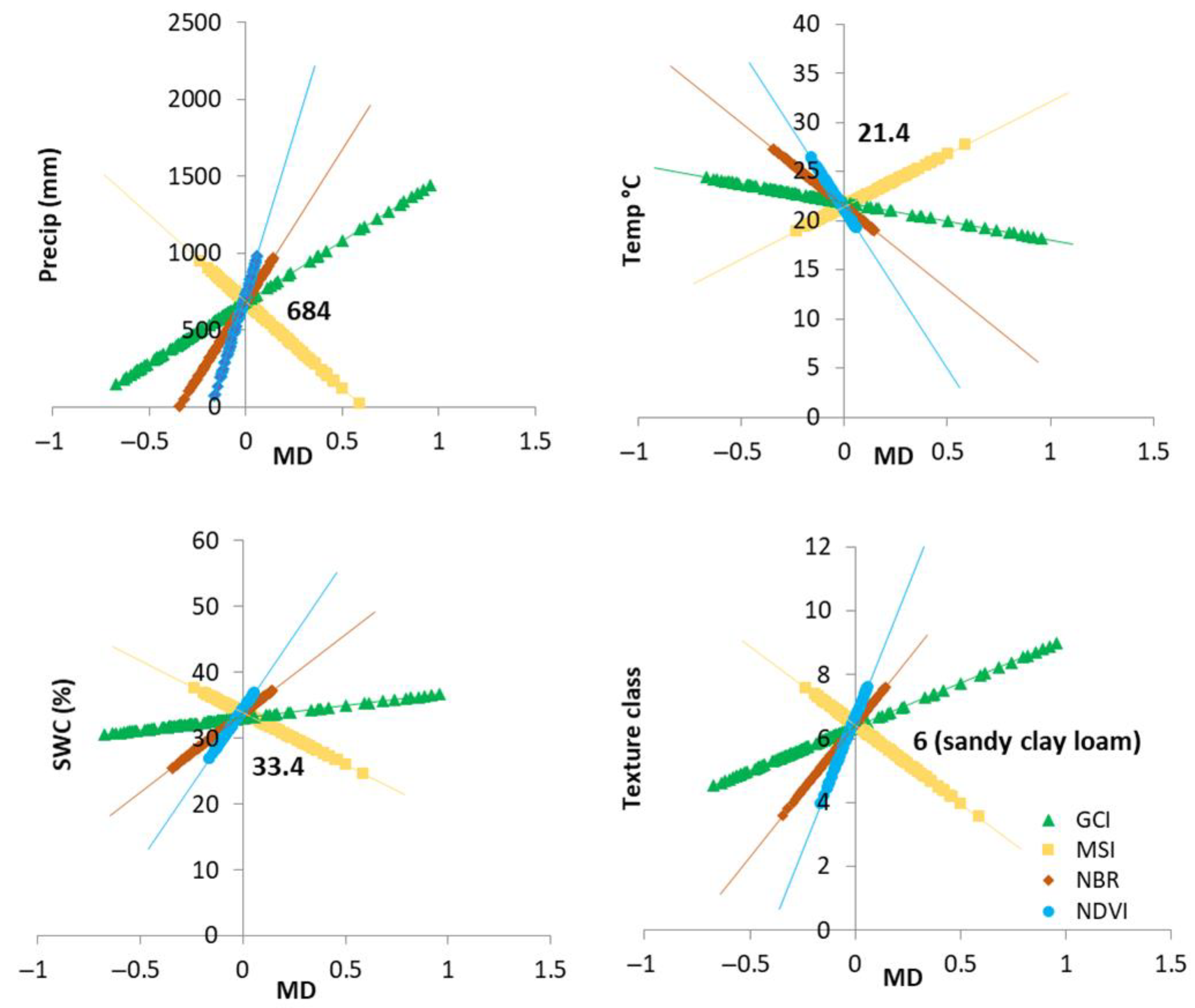
The detailed statistics for each regression model presented in
Figure 8 and
Table 6 are shown below. The regression models were fitted between the effects size (MD, mean difference between control and treatment sites) of four spectral indices and the interval-defined moderators significant in the meta-analyses. The four spectral indices considered were the GCI (
Figure A1,
Figure A2,
Figure A3 and
Figure A4), NDVI (
Figure A5,
Figure A6,
Figure A7 and
Figure A8), NBR (
Figure A9,
Figure A10,
Figure A11 and
Figure A12), and MSI (
Figure A13,
Figure A14,
Figure A15 and
Figure A16). And the four moderators studied were precipitation (Precip), temperature (Temp), soil water content (SWC), and soil texture.
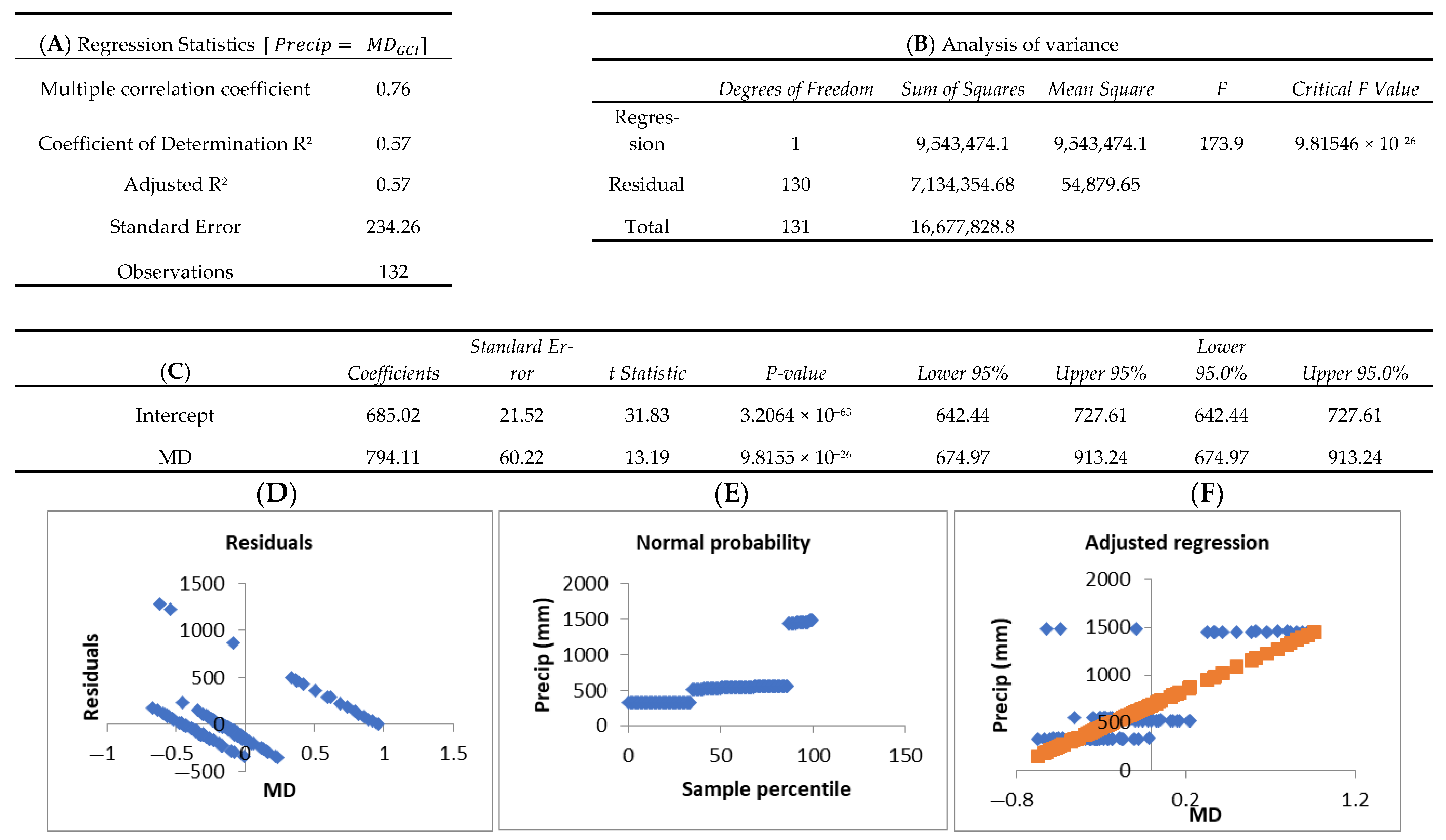
Figure A1.
Regression model fitted between the size effects of GCI (MD = mean difference between control and treatment sites) and precipitation (Precip, moderator). The basic adjustment statistics (A) are presented, along with the analysis of variance, which indicates the significance of the model (B), the model coefficients, showing the intercept, and the significance of the coefficient for MD, along with standard errors, t-values, and 95% confidence intervals (C). Residuals vs. MD plot (D), Normal probability (Q–Q) plot assessing the normality of residuals (E), and adjusted regression plot illustrating the positive relationship between MD and precipitation (F) are presented graphically.
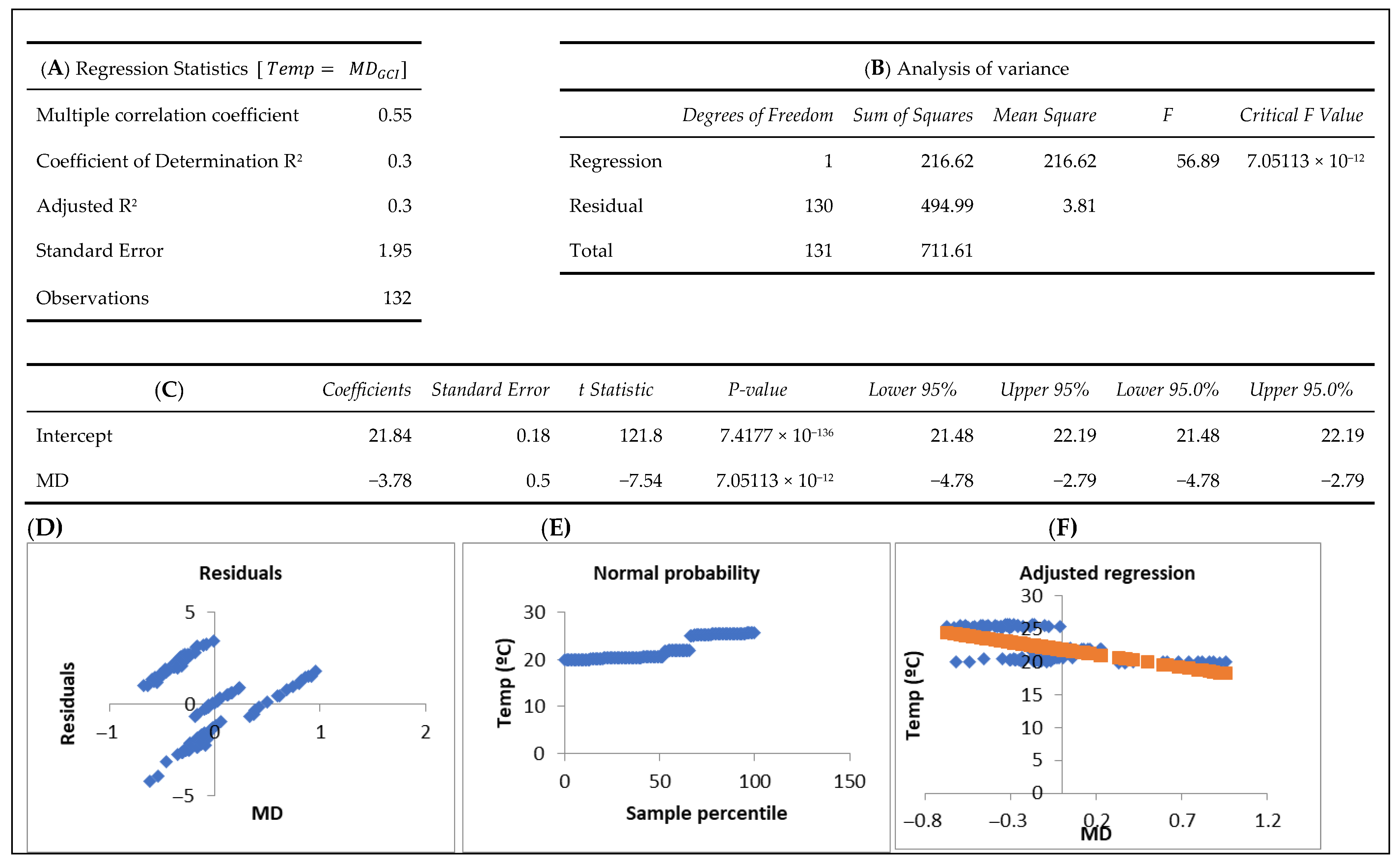
Figure A2.
Regression model fitted between the size effects of GCI (MD = mean difference between control and treatment sites) and temperature (Temp, moderator). The basic adjustment statistics (A) are presented, along with the analysis of variance, which indicates the significance of the model (B), the model coefficients, showing the intercept and the significance of the coefficient for MD, along with standard errors, t-values, and 95% confidence intervals (C). Residuals vs. MD plot (D), Normal probability (Q–Q) plot assessing the normality of residuals (E), and adjusted regression plot illustrating the negative relationship between MD and temperature (F) are presented graphically.
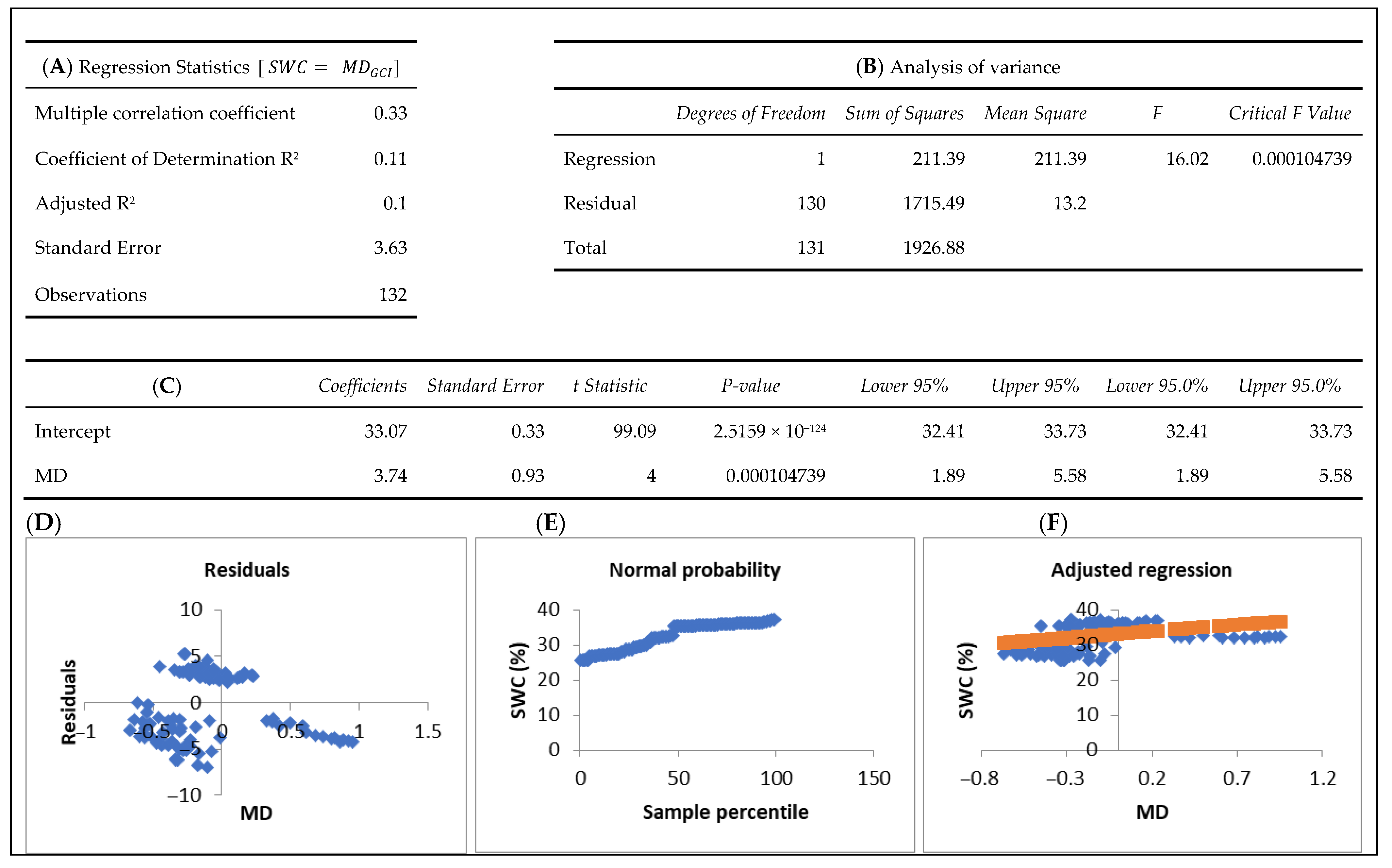
Figure A3.
Regression model fitted between the size effects of GCI (MD = mean difference between control and treatment sites) and soil water content (SWC, moderator). The basic adjustment statistics (A) are presented, along with the analysis of variance, which indicates the significance of the model (B), the model coefficients, showing the intercept and the significance of the coefficient for MD, along with standard errors, t-values, and 95% confidence intervals (C). Residuals vs. MD plot (D), Normal probability (Q–Q) plot assessing the normality of residuals, (E) and adjusted regression plot illustrating the positive relationship between MD and soil water content (F) are presented graphically.
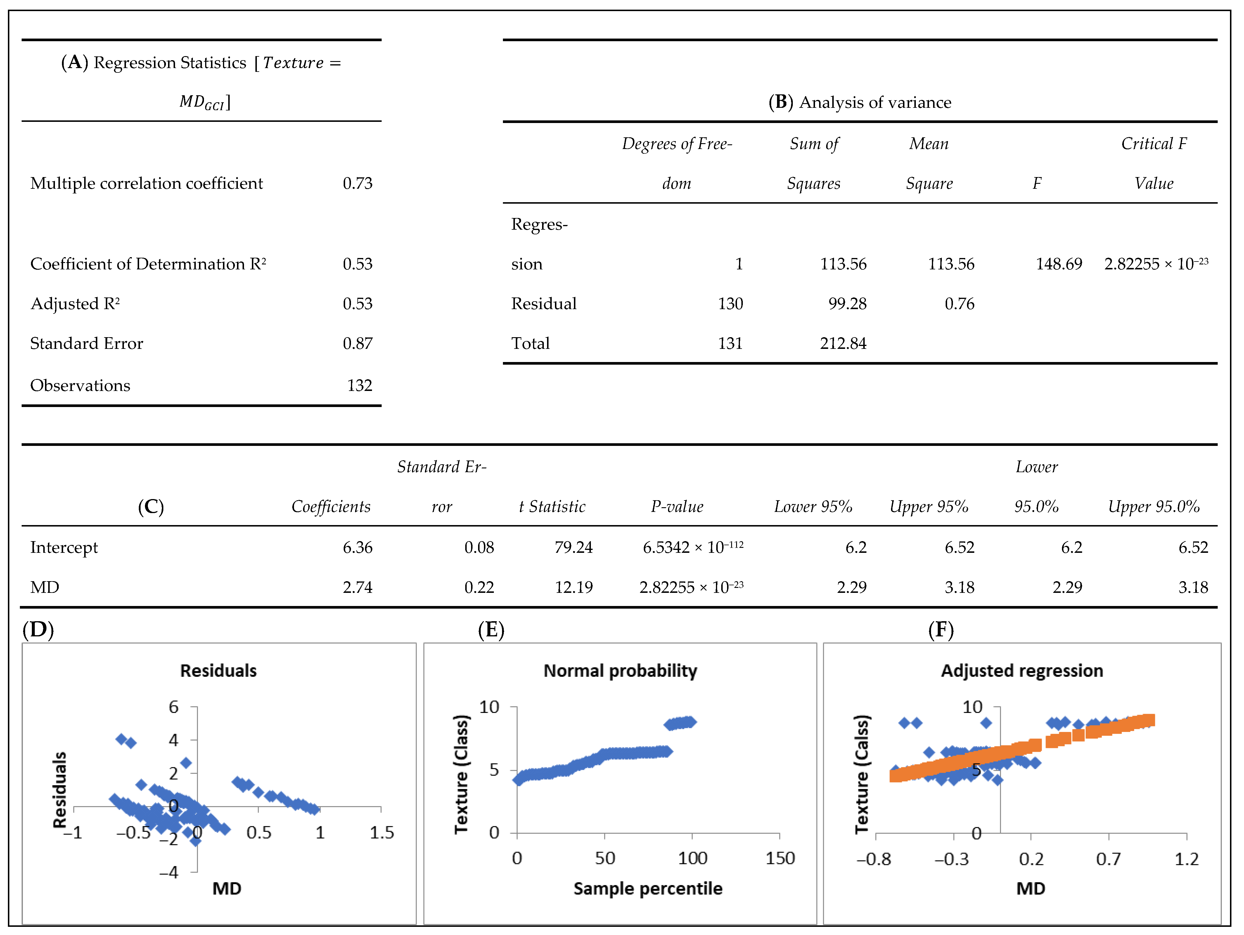
Figure A4.
Regression model fitted between the size effects of GCI (MD = mean difference between control and treatment sites) and soil texture (Texture, moderator). The basic adjustment statistics (A) are presented, along with the analysis of variance, which indicates the significance of the model (B), the model coefficients, showing the intercept and the significance of the coefficient for MD, along with standard errors, t-values, and 95% confidence intervals (C). Residuals vs. MD plot (D), Normal probability (Q–Q) plot assessing the normality of residuals (E), and adjusted regression plot illustrating the positive relationship between MD and soil texture (F) are presented graphically.
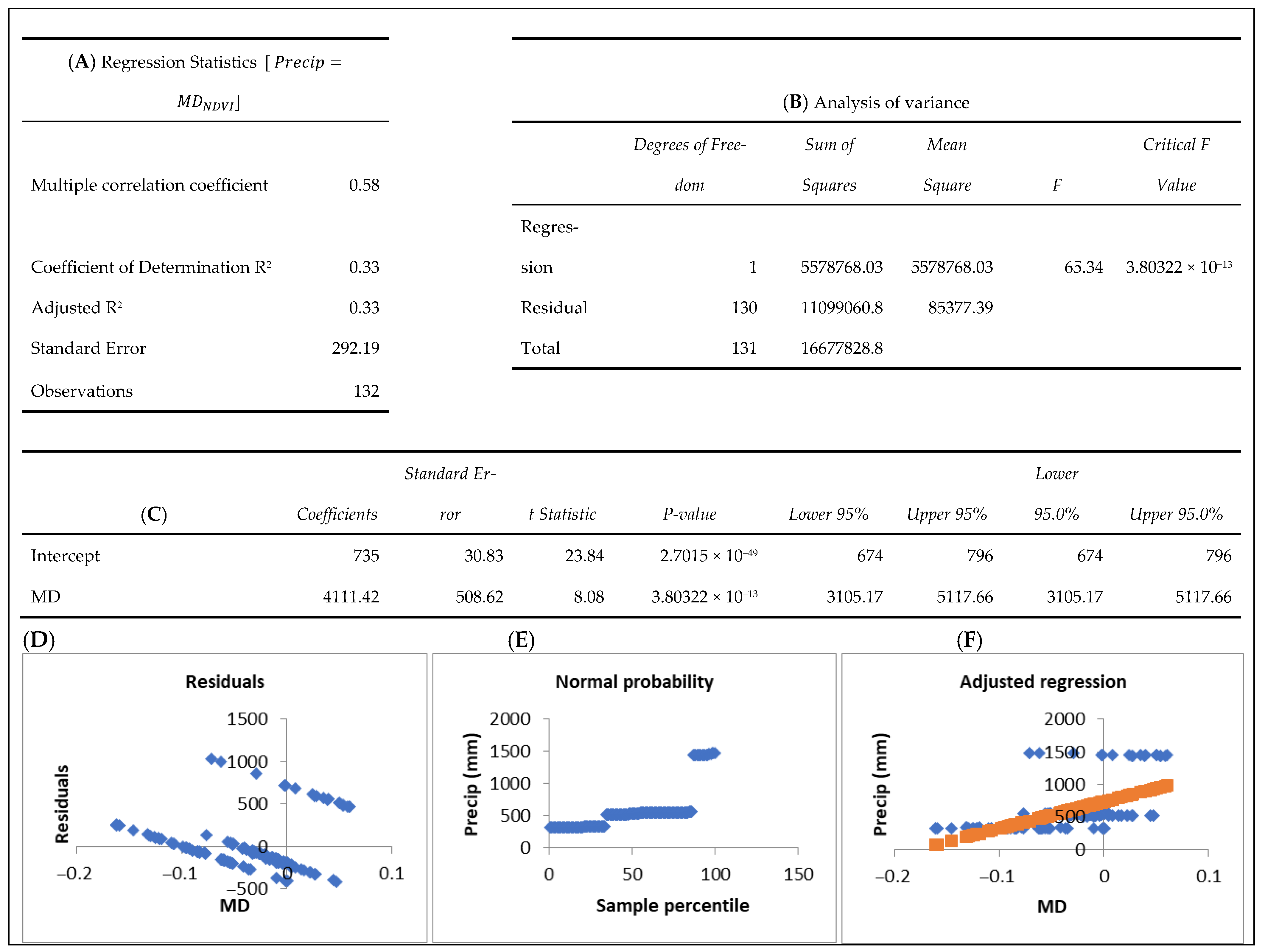
Figure A5.
Regression model fitted between the size effects of NDVI (MD = mean difference between control and treatment sites) and precipitation (Precip, moderator). The basic adjustment statistics (A) are presented, along with the analysis of variance, which indicates the significance of the model (B), the model coefficients, showing the intercept and the significance of the coefficient for MD, along with standard errors, t-values, and 95% confidence intervals (C). Residuals vs. MD plot (D), Normal probability (Q–Q) plot assessing the normality of residuals (E), and adjusted regression plot illustrating the positive relationship between MD and precipitation (F) are presented graphically.
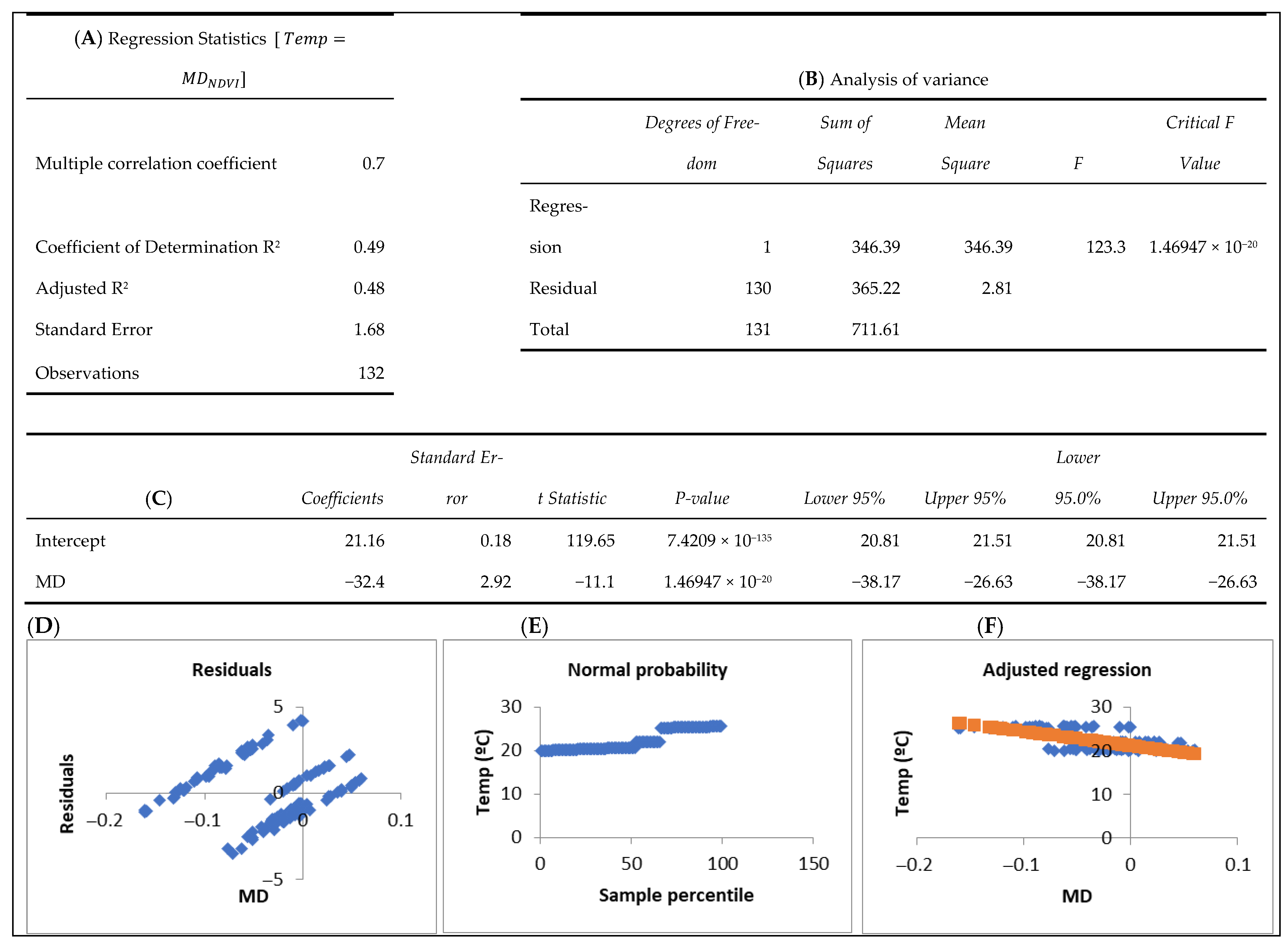
Figure A6.
Regression model fitted between the size effects of NDVI (MD = mean difference between control and treatment sites) and temperature (Temp, moderator). The basic adjustment statistics (A) are presented, along with the analysis of variance, which indicates the significance of the model (B), the model coefficients, showing the intercept and the significance of the coefficient for MD, along with standard errors, t-values, and 95% confidence intervals (C). Residuals vs. MD plot (D), Normal probability (Q–Q) plot assessing the normality of residuals (E), and adjusted regression plot illustrating the negative relationship between MD and temperature (F) are presented graphically.
Figure A7.
Regression model fitted between the size effects of NDVI (MD = mean difference between control and treatment sites) and soil water content (SWC, moderator). The basic adjustment statistics (A) are presented, along with the analysis of variance, which indicates the significance of the model (B), the model coefficients, showing the intercept and the significance of the coefficient for MD, along with standard errors, t-values, and 95% confidence intervals (C). Residuals vs. MD plot (D), Normal probability (Q–Q) plot assessing the normality of residuals (E), and adjusted regression plot illustrating the positive relationship between MD and soil water content (F) are presented graphically.
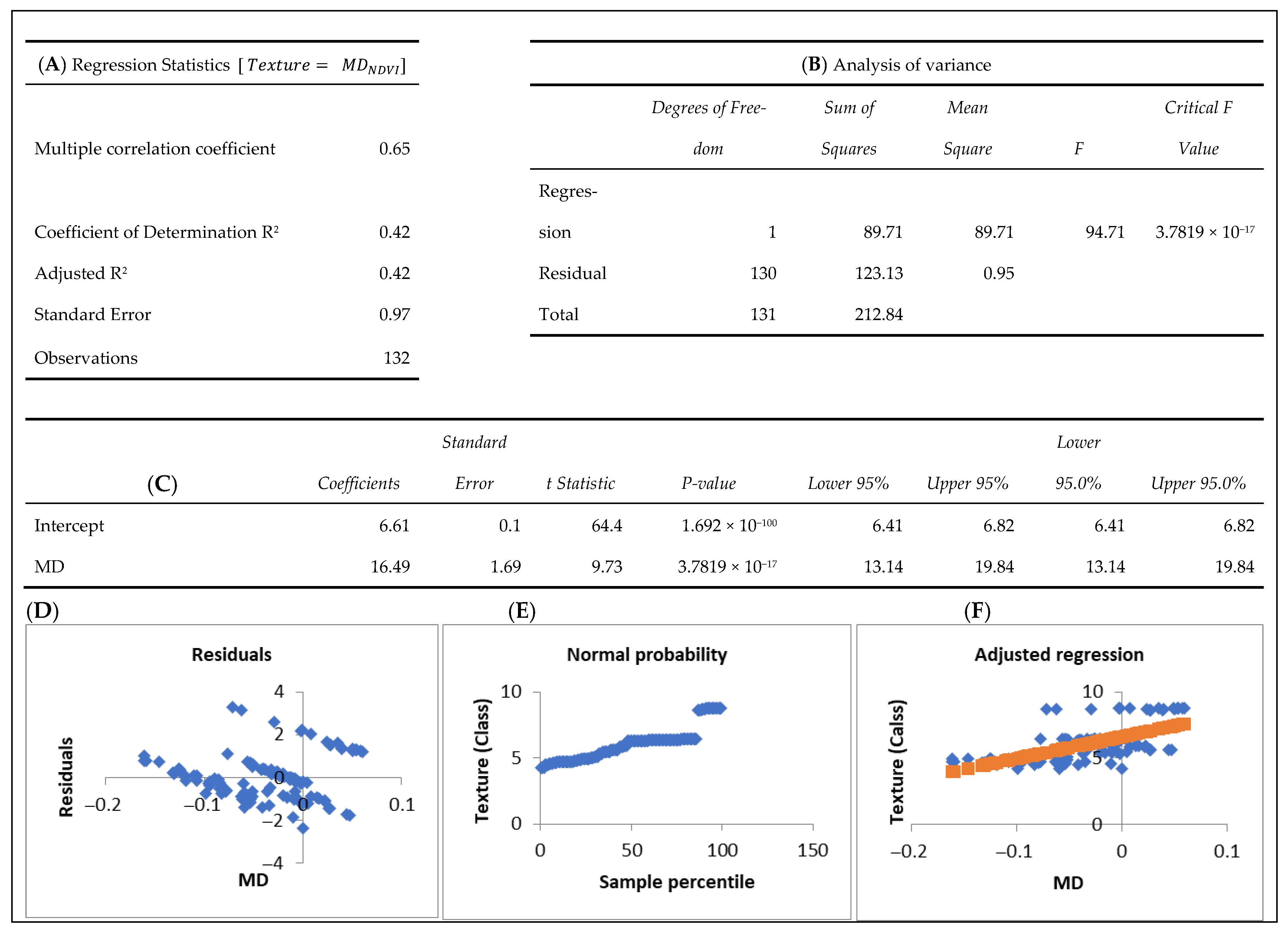
Figure A8.
Regression model fitted between the size effects of NDVI (MD = mean difference between control and treatment sites) and soil texture (Texture, moderator). The basic adjustment statistics (A) are presented, along with the analysis of variance, which indicates the significance of the model (B), the model coefficients, showing the intercept and the significance of the coefficient for MD, along with standard errors, t-values, and 95% confidence intervals (C). Residuals vs. MD plot (D), Normal probability (Q–Q) plot assessing the normality of residuals (E), and adjusted regression plot illustrating the positive relationship between MD and soil texture (F) are presented graphically.
Figure A9.
Regression model fitted between the size effects of NBR (MD = mean difference between control and treatment sites) and precipitation (Precip, moderator). The basic adjustment statistics (A) are presented, along with the analysis of variance, which indicates the significance of the model (B), the model coefficients, showing the intercept and the significance of the coefficient for MD, along with standard errors, t-values, and 95% confidence intervals (C). Residuals vs. MD plot (D), Normal probability (Q–Q) plot assessing the normality of residuals (E), and adjusted regression plot illustrating the positive relationship between MD and precipitation (F) are presented graphically.
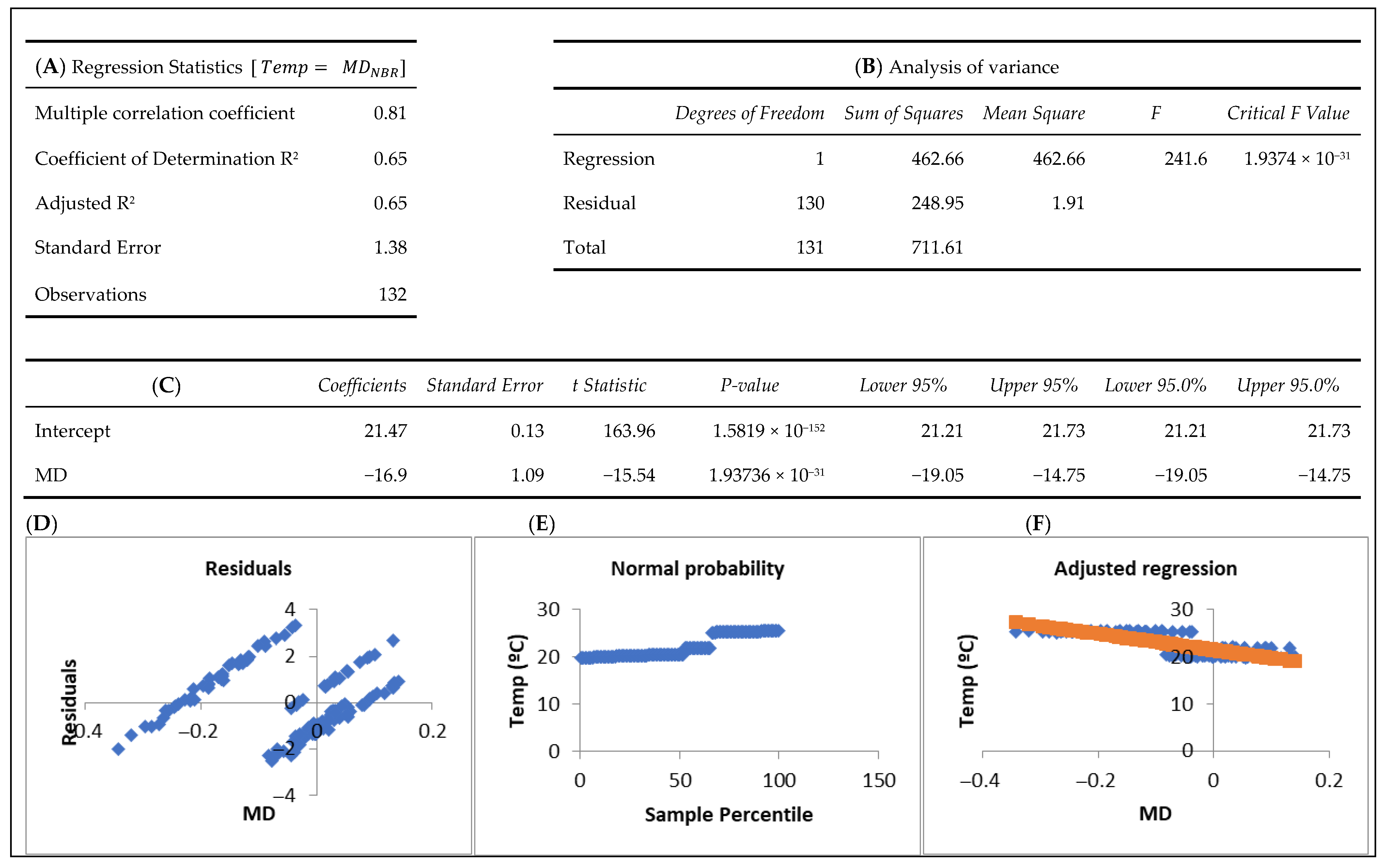
Figure A10.
Regression model fitted between the size effects of NBR (MD = mean difference between control and treatment sites) and temperature (Temp, moderator). The basic adjustment statistics (A) are presented, along with the analysis of variance, which indicates the significance of the model (B), the model coefficients, showing the intercept and the significance of the coefficient for MD, along with standard errors, t-values, and 95% confidence intervals (C). Residuals vs. MD plot (D), Normal probability (Q–Q) plot assessing the normality of residuals (E), and adjusted regression plot illustrating the negative relationship between MD and temperature (F) are presented graphically.
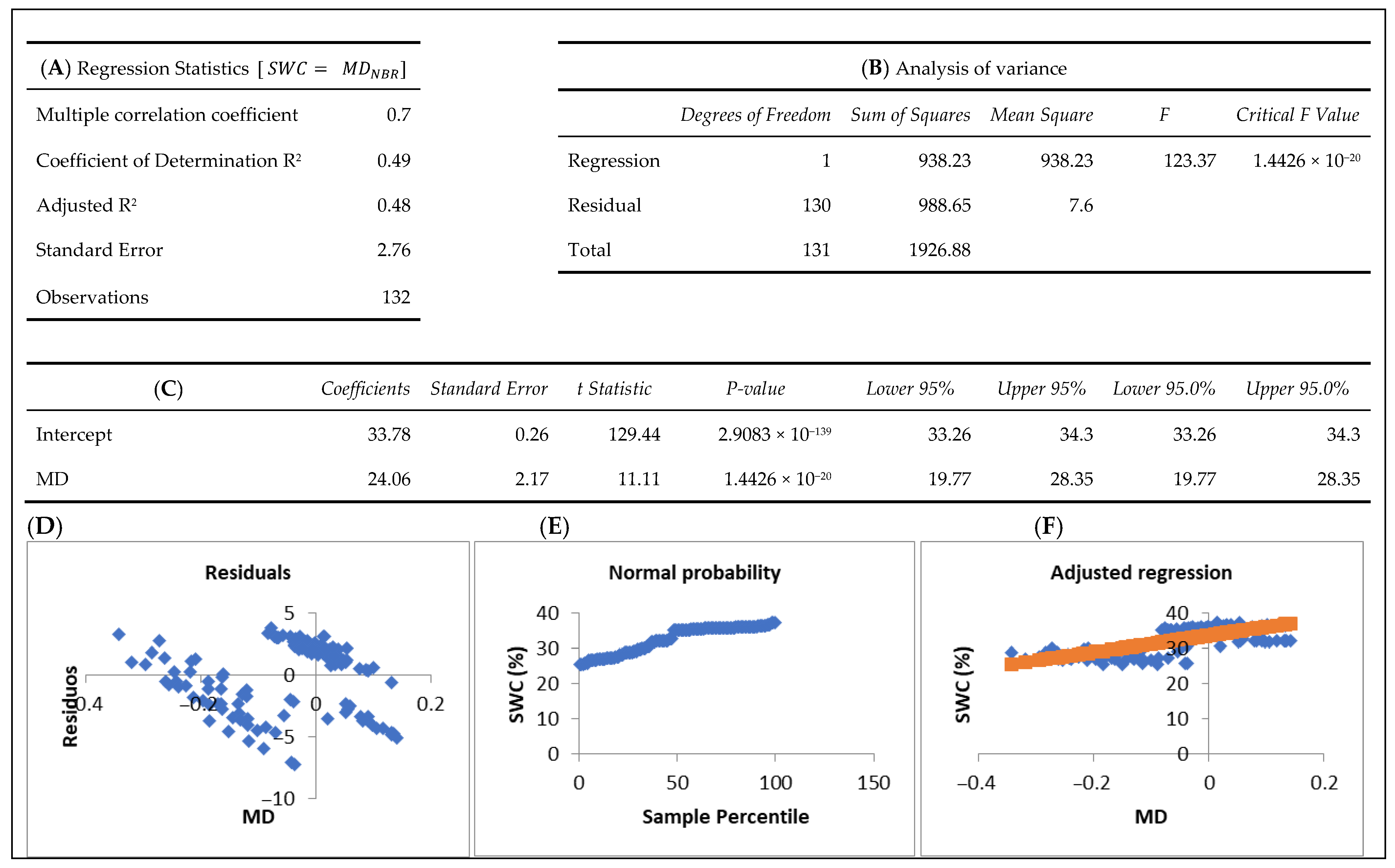
Figure A11.
Regression model fitted between the size effects of NBR (MD = mean difference between control and treatment sites) and soil water content (SWC, moderator). The basic adjustment statistics (A) are presented, along with the analysis of variance, which indicates the significance of the model (B), the model coefficients, showing the intercept and the significance of the coefficient for MD, along with standard errors, t-values, and 95% confidence intervals (C). Residuals vs. MD plot (D), Normal probability (Q–Q) plot assessing the normality of residuals (E), and adjusted regression plot illustrating the positive relationship between MD and soil water content (F) are presented graphically.
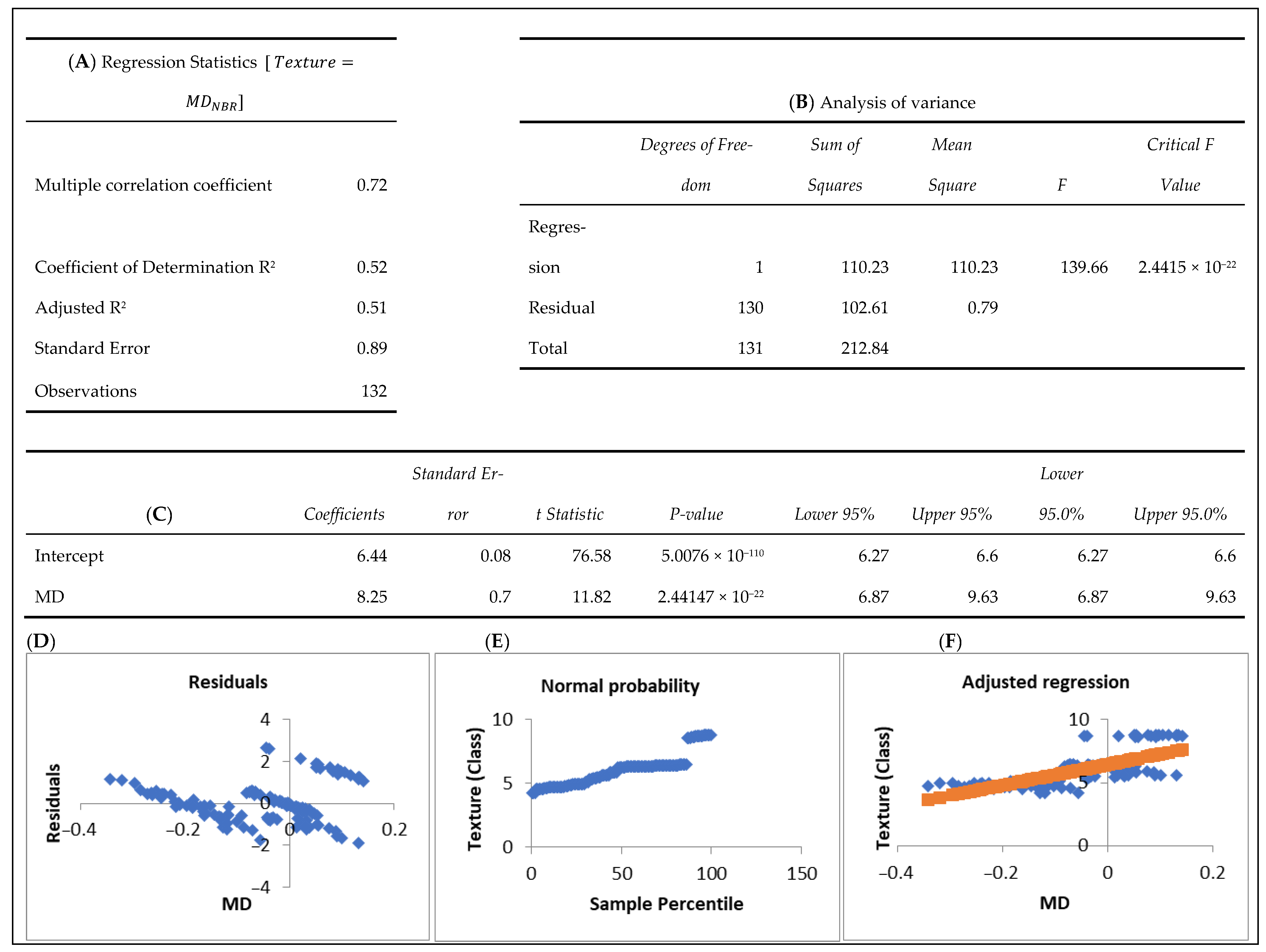
Figure A12.
Regression model fitted between the size effects of NBR (MD = mean difference between control and treatment sites) and soil texture (Texture, moderator). The basic adjustment statistics (A) are presented, along with the analysis of variance, which indicates the significance of the model (B), the model coefficients, showing the intercept and the significance of the coefficient for MD, along with standard errors, t-values, and 95% confidence intervals (C). Residuals vs. MD plot (D), Normal probability (Q–Q) plot assessing the normality of residuals (E), and adjusted regression plot illustrating the positive relationship between MD and soil texture (F) are presented graphically.
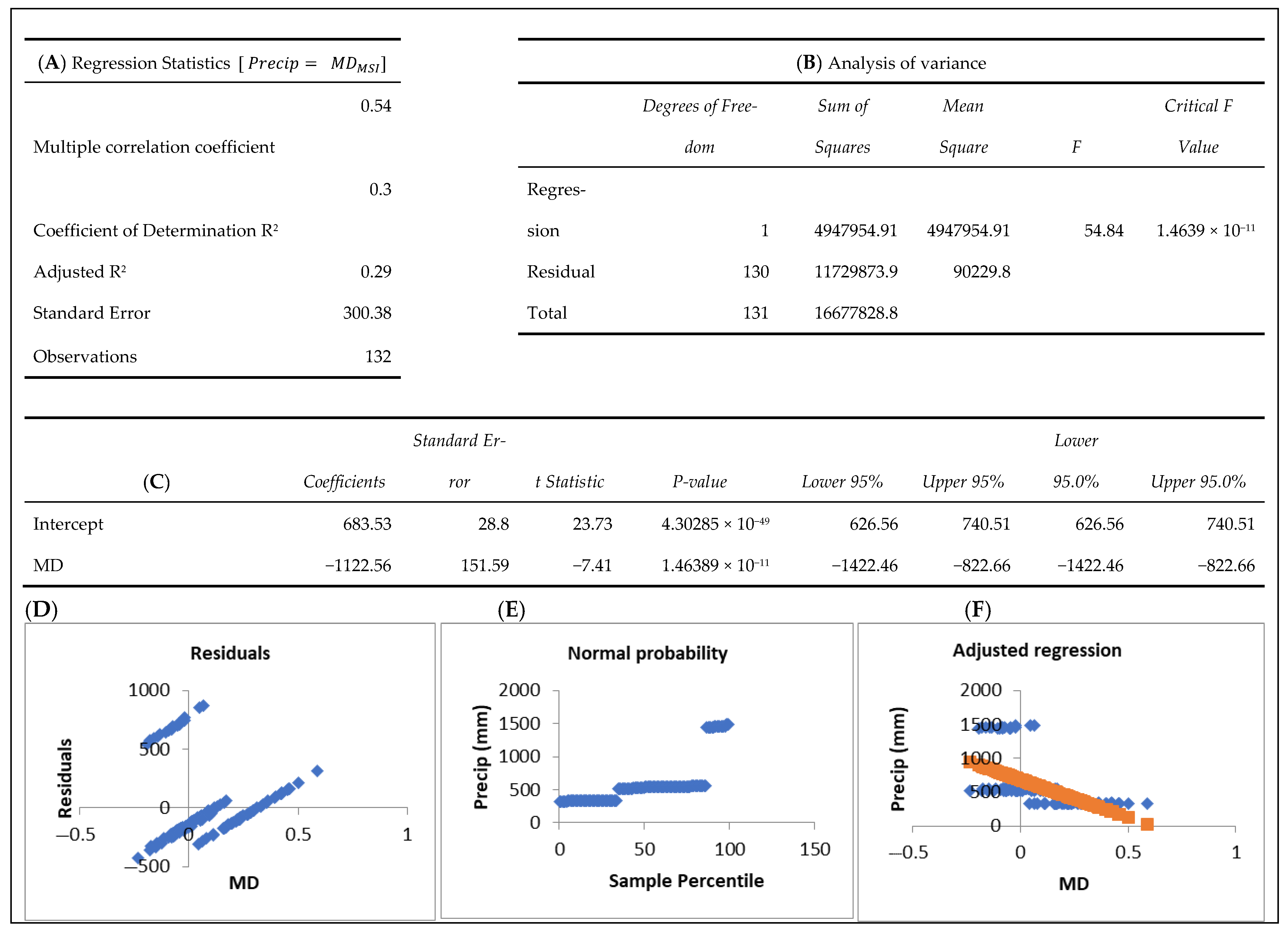
Figure A13.
Regression model fitted between the size effects of MSI (MD = mean difference between control and treatment sites) and precipitation (Precip, moderator). The basic adjustment statistics (A) are presented, along with the analysis of variance, which indicates the significance of the model (B), the model coefficients, showing the intercept and the significance of the coefficient for MD, along with standard errors, t-values, and 95% confidence intervals (C). Residuals vs. MD plot (D), Normal probability (Q–Q) plot assessing the normality of residuals (E), and adjusted regression plot illustrating the negative relationship between MD and precipitation (F) are presented graphically.
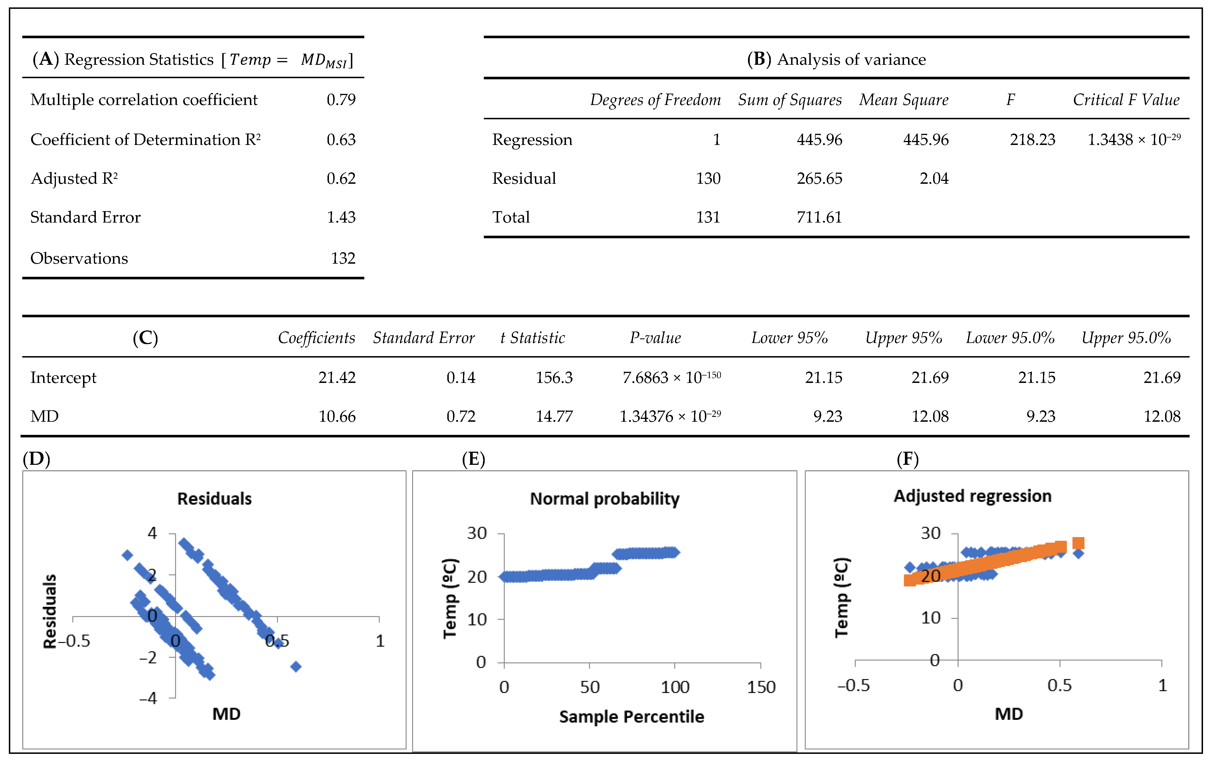
Figure A14.
Regression model fitted between the size effects of MSI (MD = mean difference between control and treatment sites) and temperature (Temp, moderator). The basic adjustment statistics (A) are presented, along with the analysis of variance, which indicates the significance of the model (B), the model coefficients, showing the intercept and the significance of the coefficient for MD, along with standard errors, t-values, and 95% confidence intervals (C). Residuals vs. MD plot (D), Normal probability (Q–Q) plot assessing the normality of residuals (E), and adjusted regression plot illustrating the positive relationship between MD and temperature (F) are presented graphically.
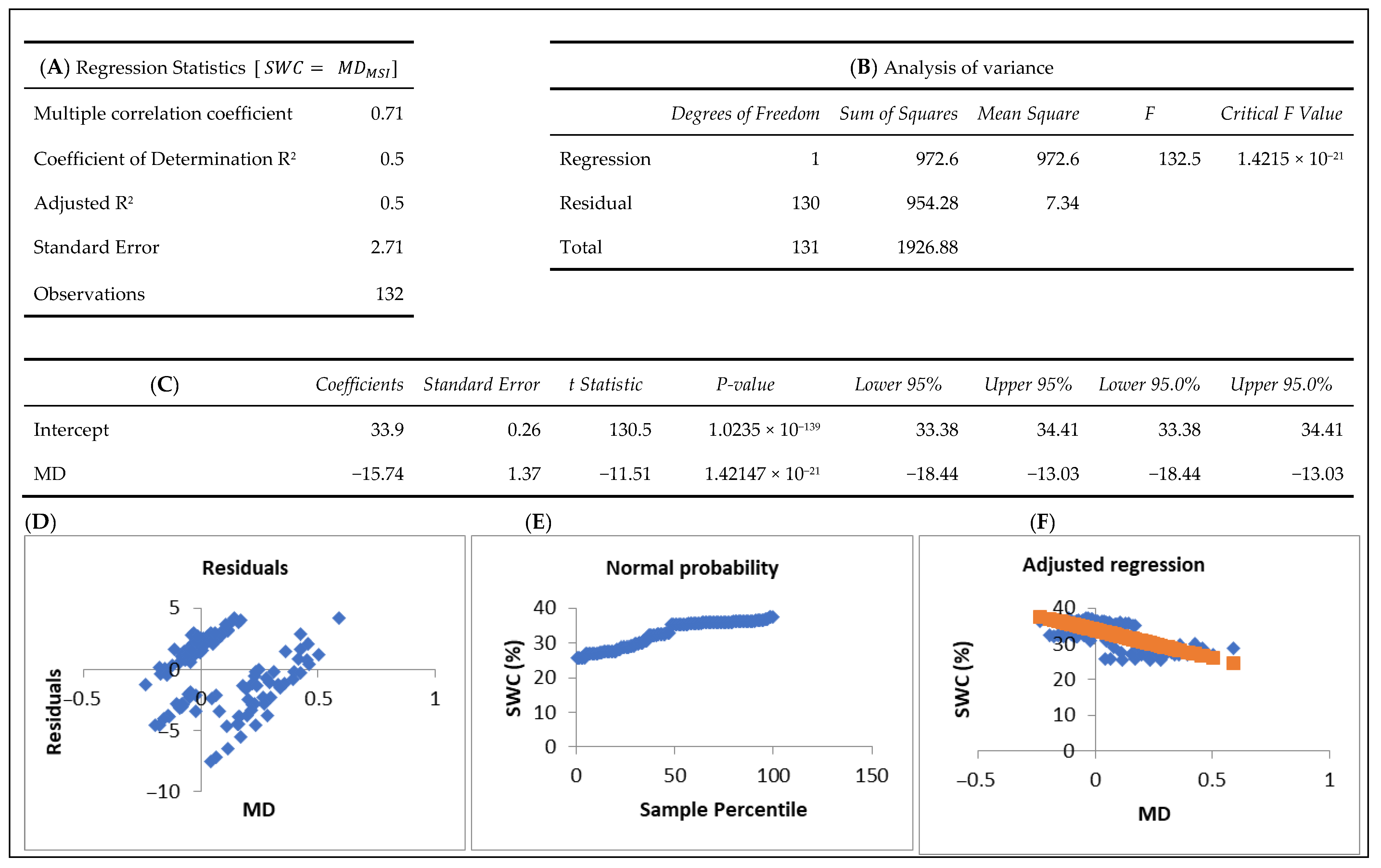
Figure A15.
Regression model fitted between the size effects of MSI (MD = mean difference between control and treatment sites) and soil water content (SWC, moderator). The basic adjustment statistics (A) are presented, along with the analysis of variance, which indicates the significance of the model (B), the model coefficients, showing the intercept and the significance of the coefficient for MD, along with standard errors, t-values, and 95% confidence intervals (C). Residuals vs. MD plot (D), Normal probability (Q–Q) plot assessing the normality of residuals (E), and adjusted regression plot illustrating the negative relationship between MD and soil water content (F) are presented graphically.
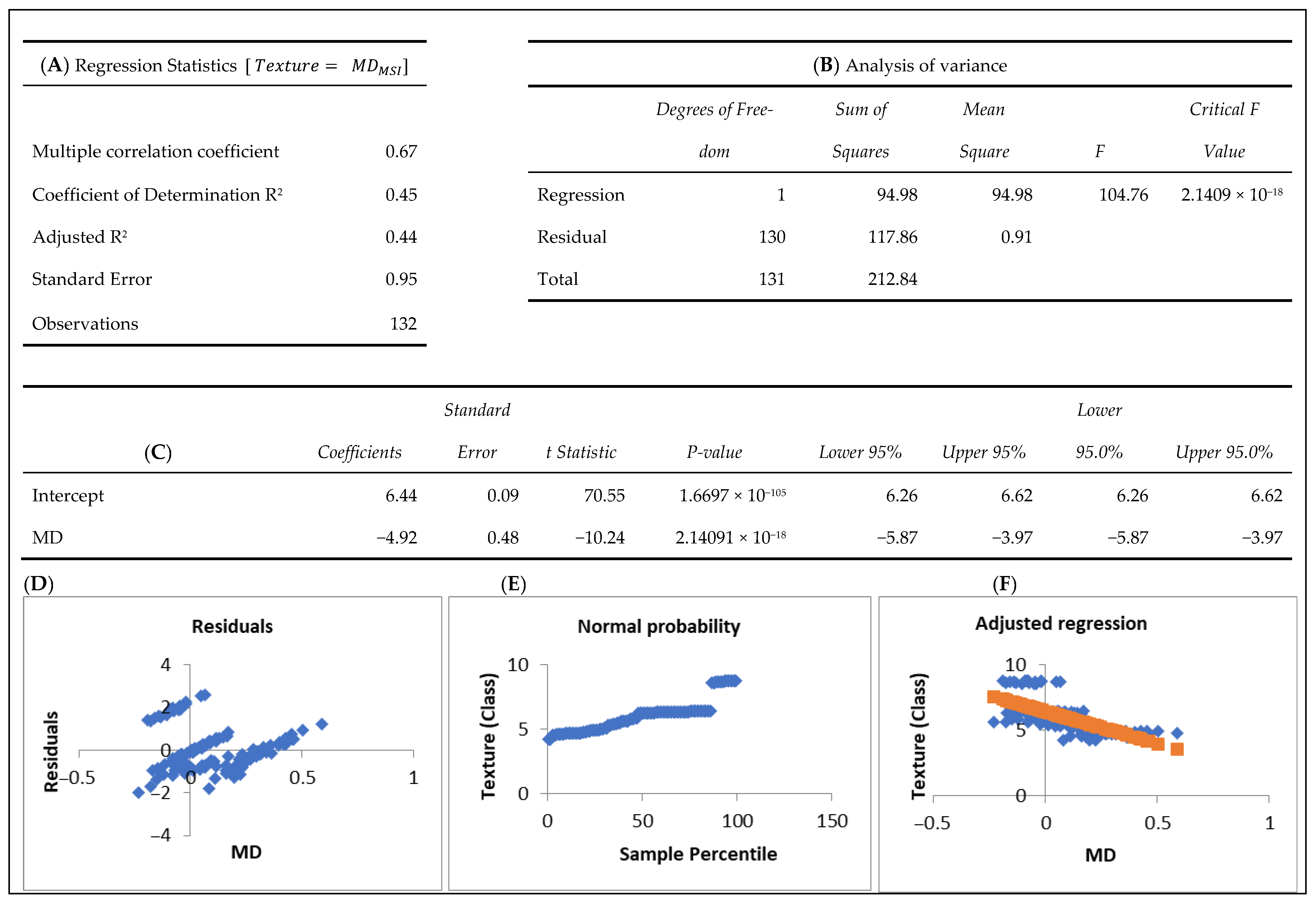
Figure A16.
Regression model fitted between the size effects of MSI (MD = mean difference between control and treatment sites) and soil texture (Texture, moderator). The basic adjustment statistics (A) are presented, along with the analysis of variance, which indicates the significance of the model (B), the model coefficients, showing the intercept and the significance of the coefficient for MD, along with standard errors, t-values, and 95% confidence intervals (C). Residuals vs. MD plot (D), Normal probability (Q–Q) plot assessing the normality of residuals (E), and adjusted regression plot illustrating the negative relationship between MD and soil texture (F) are presented graphically.


 ,
, 

