
The Impact of Increasing Tree Cover on Landscape Metrics and Connectivity: A Cellular Automata Modelling Approach


Abstract
1. Introduction
2. Materials and Methods
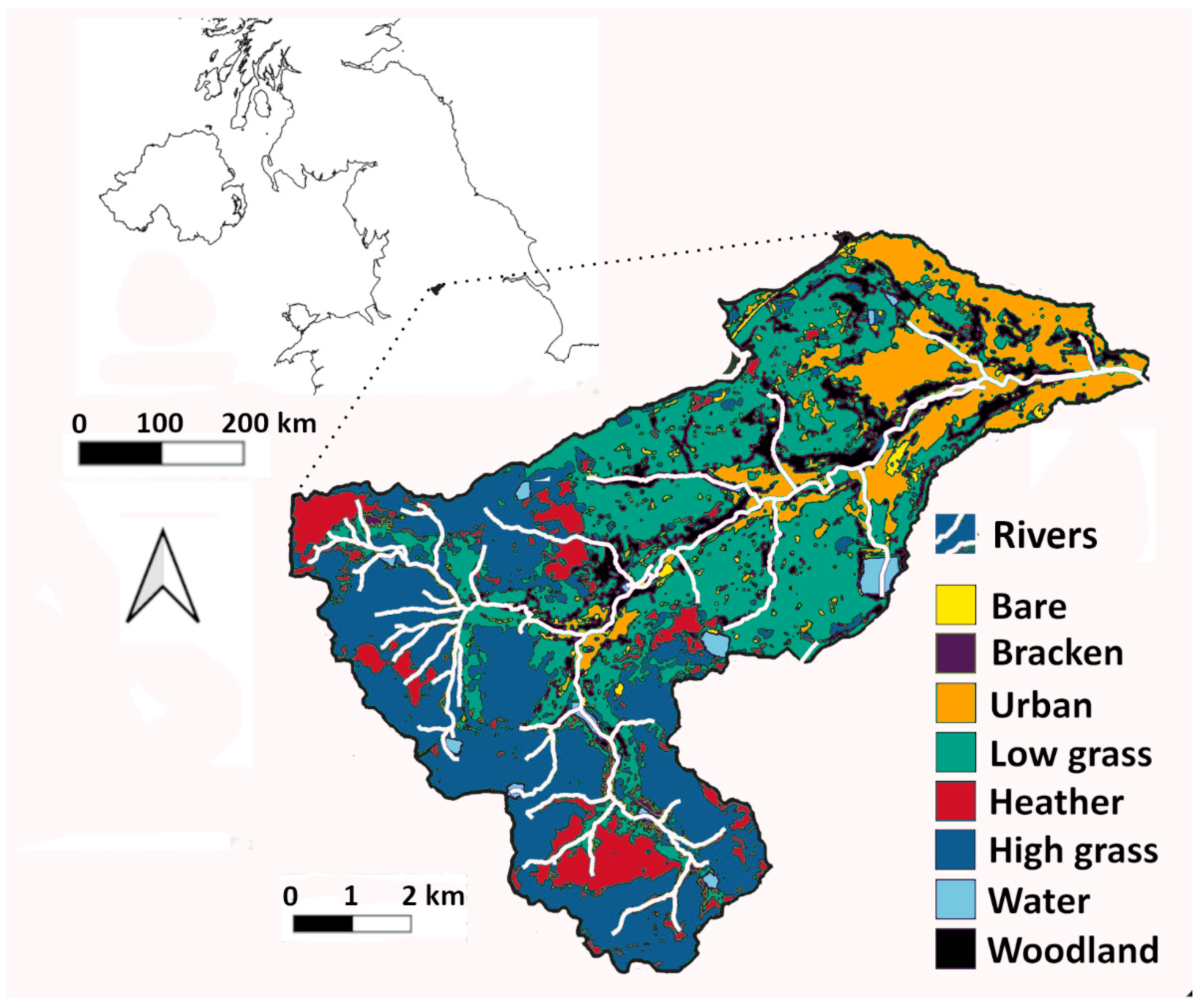
2.1. Study Site
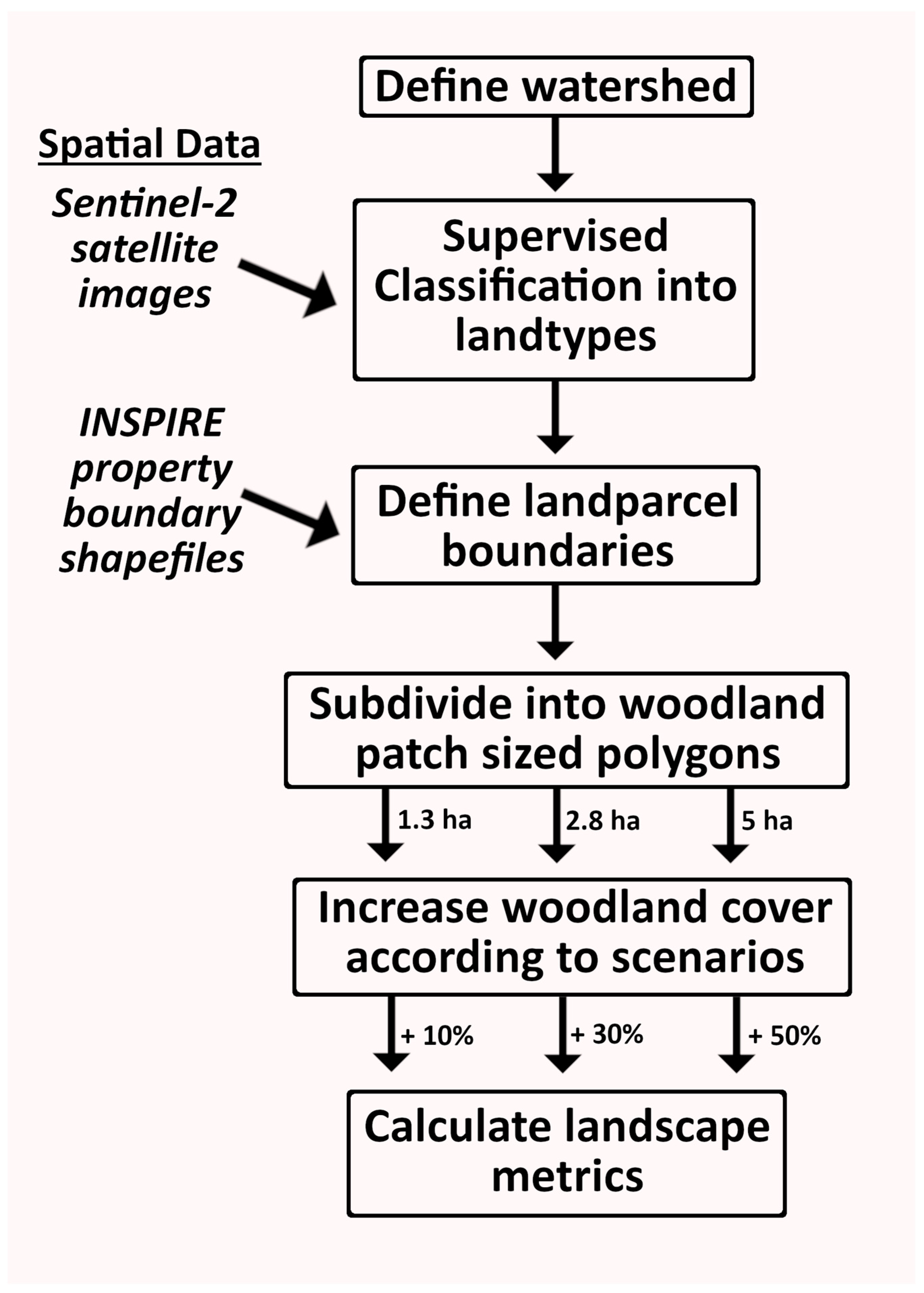
2.2. Landcover Maps
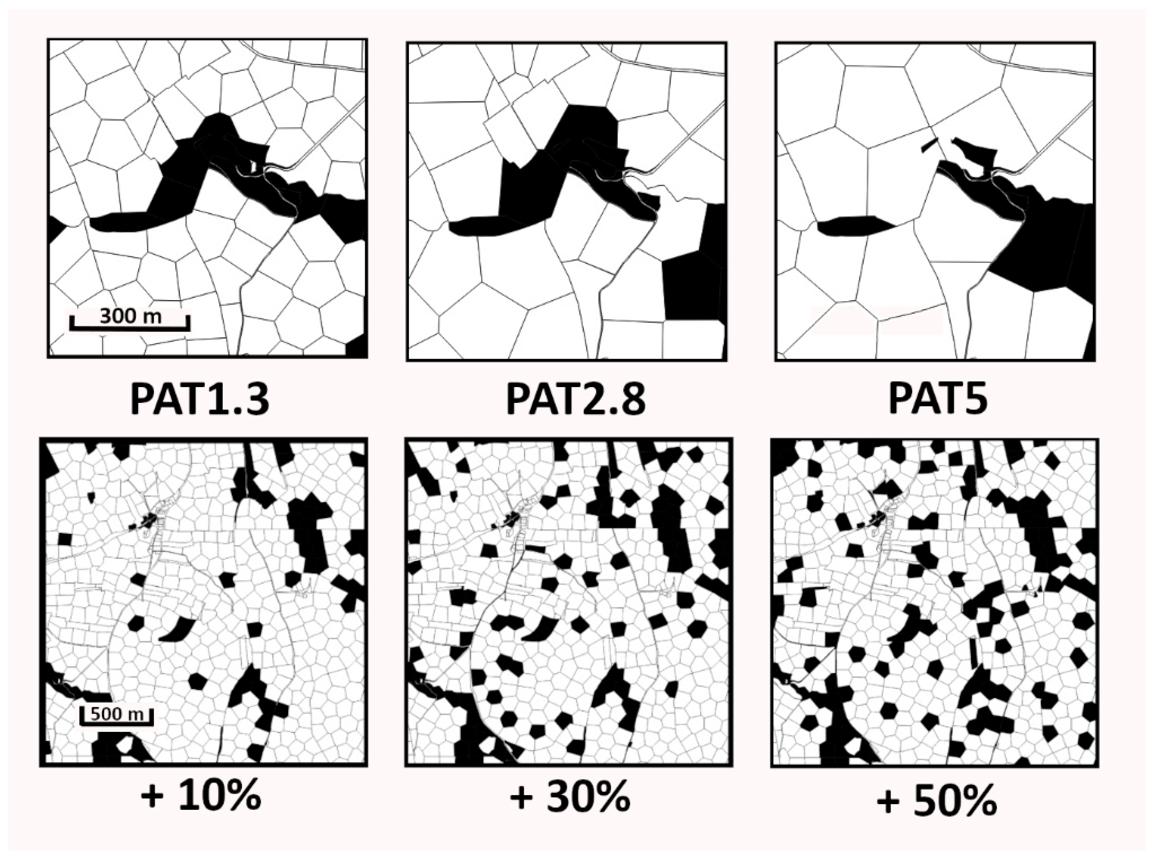
2.3. Polygonisation
2.4. Woodland Creation Scenarios
2.5. Landscape Metric Calculation
3. Results
3.1. Baseline Data
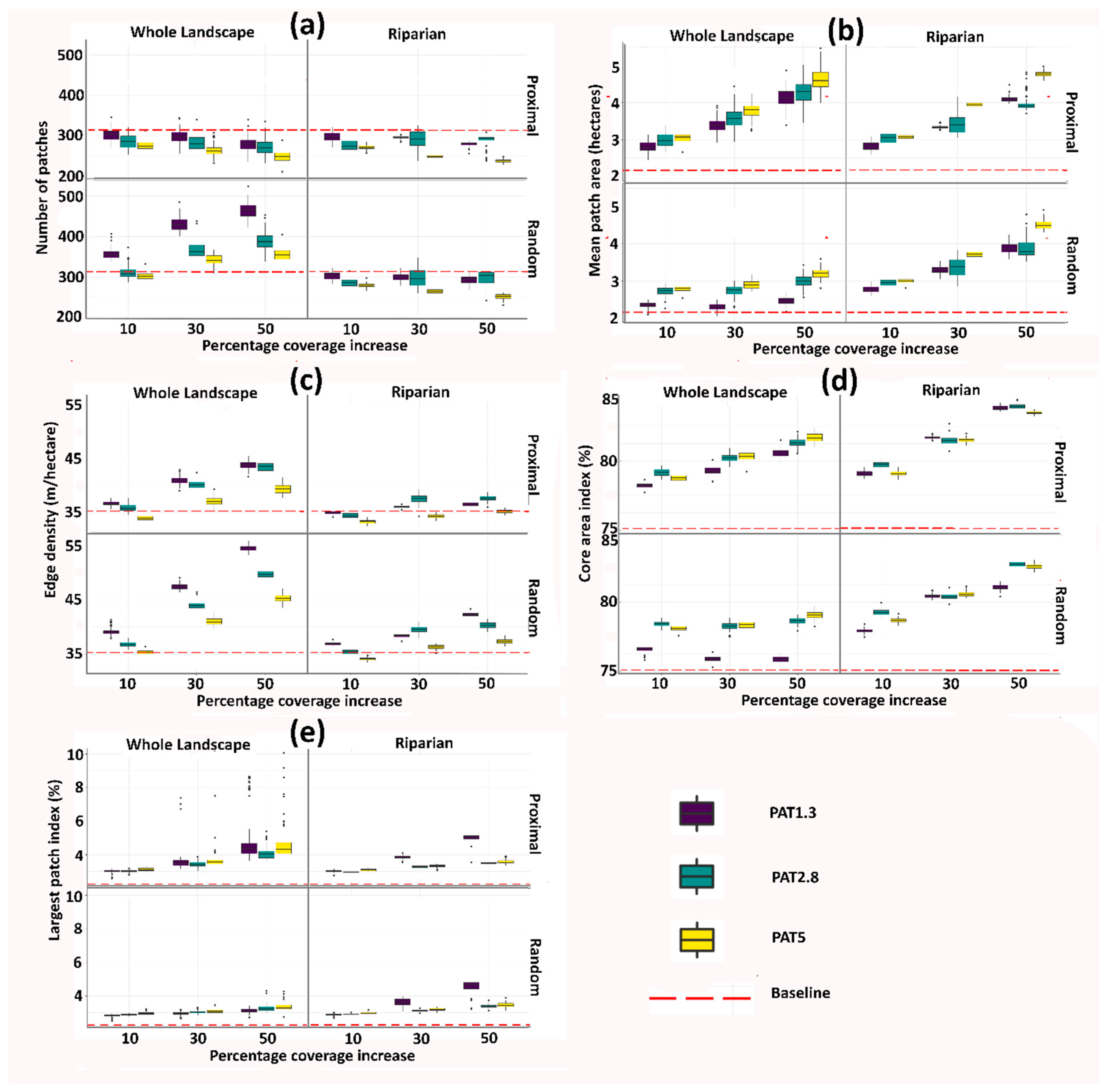
3.2. Landscape Metrics
4. Discussion
4.1. SLOSS
4.2. Connectivity and Shape
4.3. UK Woodland Expansion Target
4.4. Considerations
Supplementary Materials
Author Contributions
Funding
Data Availability Statement
Conflicts of Interest
Abbreviations
| OS | Ordnance Survey |
| SLOSS | Single Large or Several Small |
| SLASS | Single Large and Several Small |
References
- Eurostat. EU Forestry Database. 2022. Available online: https://ec.europa.eu/eurostat/web/forestry/database (accessed on 6 March 2024).
- Forestry Commission. Forestry Commission Open Data. 2024. Available online: https://data-forestry.opendata.arcgis.com/ (accessed on 20 February 2024).
- DEFRA. Environmental Targets Consultation Summary of Responses and Government Response. Department for Environment, Food & Rural Affairs Report 16/12/2022. 2022. Available online: www.gov.uk/government/publications (accessed on 7 March 2024).
- Bradfer-Lawrence, T.; Finch, T.; Bradbury, R.B.; Buchanan, G.M.; Midgley, A.; Field, R.H. The potential contribution of terrestrial nature-based solutions to a national ‘net zero’ climate target. J. Appl. Ecol. 2021, 58, 2349–2360. [Google Scholar] [CrossRef]
- Herbert, S.; Hotchkiss, A.; Reid, C.; Hornigold, K. Woodland Creation Guide; Woodland Trust: Grantham, UK, 2022. [Google Scholar]
- Cooper, M.; Patil, S.; Nisbet, T.R.; Thomas, H.; Smith, A.; McDonald, M. Role of forested land for natural flood management in the UK: A review. WIREs Water 2021, 8, e1541. [Google Scholar] [CrossRef]
- Forestry Commission. UK Forestry Standard Practice Guide: Designing and Managing Forests and Woodlands to Reduce Flood Risk. 2022. Available online: www.forestresearch.gov.uk/publications (accessed on 5 June 2025).
- Hopkins, J.J.; Kirby, K.J. Ecological change in British broadleaved woodland since 1947. Ibis 2007, 149, 29–40. [Google Scholar] [CrossRef]
- Fahrig, L. Effects of habitat fragmentation on biodiversity. Ann. Rev. Ecol. Syst. 2003, 34, 487–515. [Google Scholar] [CrossRef]
- Kolb, A.; Lindhorst, S. Forest fragmentation and plant reproductive success: A case study in four perennial herbs. Plant Ecol. 2006, 185, 209–220. [Google Scholar] [CrossRef]
- Mullu, D. A review on the effect of habitat fragmentation on ecosystem. J. Nat. Sci. Res. 2016, 6, 1–15. [Google Scholar]
- Hill, J.L.; Curran, P.J. Species composition in fragmented forests: Conservation implications of changing forest area. Appl. Geogr. 2001, 21, 157–174. [Google Scholar] [CrossRef]
- Van Langevelde, F. Scale of habitat connectivity and colonization in fragmented nuthatch populations. Ecography 2000, 23, 614–622. [Google Scholar] [CrossRef]
- Yaynemsa, K.G. Single Large or Several Small (SLOSS). In Plant Biodiversity Conservation in Ethiopia; Springer: Cham, Switzerland, 2022. [Google Scholar] [CrossRef]
- Fahrig, L. Ecological responses to habitat fragmentation per se. Annu. Rev. Ecol. Evol. Syst. 2017, 48, 1–23. [Google Scholar] [CrossRef]
- Dolman, P.M.; Hinsley, S.A.; Bellamy, P.E.; Watts, K. Woodland birds in patchy landscapes: The evidence base for strategic networks. Ibis 2007, 149, 146–160. [Google Scholar] [CrossRef]
- Fahrig, L. Why do several small patches hold more species than few large patches? Glob. Ecol. Biogeogr. 2020, 29, 615–628. [Google Scholar] [CrossRef]
- Taylor, P.D.; Fahrig, L.; Henein, K.; Merriam, G. Connectivity is a vital element of landscape structure. Oikos 1993, 68, 571. [Google Scholar] [CrossRef]
- Jaeger, J.A. Landscape division, splitting index, and effective mesh size: New measures of landscape fragmentation. Landsc. Ecol. 2000, 15, 115–130. [Google Scholar] [CrossRef]
- McGarigal, K.; Cushman, S.A.; Neel, M.C.; Ene, E. FRAGSTATS: Spatial Pattern Analysis Program for Categorical Maps. 2002. Available online: http://fragstats.org (accessed on 5 June 2025).
- Cushman, S.A.; McGarigal, K. Metrics and Models for Quantifying Ecological Resilience at Landscape Scales. Front. Ecol. Evol. 2019, 7, 440. [Google Scholar] [CrossRef]
- Westaway, S.; Grange, I.; Smith, J.; Smith, L.G. Meeting tree planting targets on the UK’s path to net-zero: A review of lessons learnt from 100 years of land use policies. Land Use Policy 2023, 125, 1065021. [Google Scholar] [CrossRef]
- Flack, J.; Lukac, M.; Todman, L. Woodland planting on UK pasture land is not economically feasible, yet is more profitable than some traditional farming practices. Cent. Eur. For. J. 2022, 68, 61–71. [Google Scholar] [CrossRef]
- Peterken, G.F. Rebuilding networks of forest habitats in lowland England. Landsc. Res. 2000, 25, 291–303. [Google Scholar] [CrossRef]
- Peterken, G.F. Reversing the Habitat Fragmentation of British Woodlands; WWF-UK: Godalming, UK, 2002. [Google Scholar]
- Watts, K.; Hughes, S. Fragmentation impacts may be mixed for conservation but generally bad for restoration. Restor. Ecol. 2024, 32, e14260. [Google Scholar] [CrossRef]
- Lawton, J.H.; Brotherton, P.N.M.; Brown, V.K.; Elphick, C.; Fitter, A.H.; Forshaw, J.; Haddow, R.W.; Hilborne, S.; Leafe, R.N.; Mace, G.M.; et al. Making Space for Nature: A Review of England’s Wildlife Sites and Ecological Network. Report to Defra. 2010. Available online: http://webarchive.nationalarchives.gov.uk/20150304232731/http://assets.kew.org/files/Making%20Space%20For%20Nature%20-%20The%20Lawton%20Report.pdf (accessed on 13 March 2024).
- Kirby, K.J. What sort of treescapes do we want in Britain and what can we reasonably expect: A personal reflection. Arboric. J. 2018, 40, 39–46. [Google Scholar] [CrossRef]
- Duguma, L.A.; Minang, P.A.; Aynekulu, B.E.; Carsan, S.; Nzyoka, J.; Bah, A.; Jamnadass, R.H. From Tree Planting to Tree Growing: Rethinking Ecosystem Restoration Through Tree; ICRAF Working Paper No 304; World Agroforestry: Nairobi, Kenya, 2020. [Google Scholar] [CrossRef]
- Davies, Z.G.; Pullin, A.S. Are hedgerows effective corridors between fragments of woodland habitat? An evidence-based approach. Landsc. Ecol. 2007, 22, 333–351. [Google Scholar] [CrossRef]
- Carlier, J.; Moran, J.; Aughney, T.; Roche, N. Effects of greenway development on functional connectivity for bats. Glob. Ecol. Conserv. 2019, 18, e00613. [Google Scholar] [CrossRef]
- Hutchins, M.; Qu, Y.; Seifert-Dähnn, I.; Levin, G. Comparing likely effectiveness of urban Nature-based Solutions worldwide: The example of riparian tree planting and water quality. J. Environ. Manag. 2024, 351, 119950. [Google Scholar] [CrossRef] [PubMed]
- Lowrance, R.; Altier, L.S.; Newbold, J.D.; Schnabel, R.R.; Groffman, P.M.; Denver, J.M.; Correll, D.L.; Gilliam, J.W.; Robinson, J.L. Water quality functions of riparian forest buffers in Chesapeake Bay watersheds. Environ. Manag. 1997, 21, 687–712. [Google Scholar] [CrossRef]
- Sinokrot, B.A.; Stefan, H.G. Stream temperature dynamics: Measurements and modeling. Water Resour. Res. 1993, 29, 2299–2312. [Google Scholar] [CrossRef]
- Crick, H.Q.P.; Crosher, I.E.; Mainstone, C.P.; Taylor, S.D.; Wharton, A.; Langford, P.; Larwood, J.; Lusardi, J.; Appleton, D.; Brotherton, P.N.M.; et al. Nature Networks: A Summary for Practitioners. Natural England Research Report NERR082; Natural England: York, UK, 2020. [Google Scholar]
- Dolman, P.M.; Fuller, R.J. The Processes of Species Colonisation in Wooded Landscapes: A Review of Principles. In The Restoration of Wooded Landscapes; Humphrey, J., Newton, A., Latham, J., Gray, H., Kirby, K.H., Poulsom, E., Quine, C., Eds.; Forestry Commission: Edinburgh, Scotland, 2003; pp. 25–36. [Google Scholar]
- Mancini, F.; Hodgson, J.A.; Isaac, N.J.B. Co-designing an Indicator of Habitat Connectivity for England. Front. Ecol. Evol. 2022, 10, 892987. [Google Scholar] [CrossRef]
- Manzoor, S.A.; Griffiths, G.; Latham, J.; Lukac, M. Scenario-led modelling of broadleaf forest expansion in WalesR. Soc. Open Sci. 2019, 6, 190026. [Google Scholar] [CrossRef]
- van Strien, M.J.; Slager, C.T.J.; de Vries, B.; Grêt-Regamey, A. An improved neutral landscape model for recreating real landscapes and generating landscape series for spatial ecological simulations. Ecol. Evol. 2016, 6, 3808–3821. [Google Scholar] [CrossRef]
- Synes, N.W.; Ponchon, A.; Palmer, S.C.F.; Osborne, P.E.; Bocedi, G.; Travis, J.M.J.; Watts, K. Prioritising conservation actions for biodiversity: Lessening the impact from habitat fragmentation and climate change. Biol. Conserv. 2020, 252, 108819. [Google Scholar] [CrossRef]
- Burton, V.; Moseley, D.; Brown, C.; Metzger, M.J.; Bellamy, P. Reviewing the evidence base for the effects of woodland expansion on biodiversity and ecosystem services in the United Kingdom. For. Ecol. Manag. 2018, 430, 366–379. [Google Scholar] [CrossRef]
- Verburg, P.H.; Kok, K.; Pontius, R.G.; Veldkamp, A. Modeling Land-Use and Land-Cover Change. In Land-Use and Land-Cover Change: Global Change—The IGBP Series; Lambin, E.F., Geist, H., Eds.; Springer: Berlin/Heidelberg, Germany, 2006. [Google Scholar]
- Iversen, S.V.; MacDonald, M.A.; van der Velden, N.; van Soesbergen, A.; Convery, I.; Mansfield, L.; Holt, C.D.S. Using the Ecosystem Services assessment tool TESSA to balance the multiple landscape demands of increasing woodlands in a UK national park. Ecosyst. Serv. 2024, 68, 101644. [Google Scholar] [CrossRef]
- Copernicus. Copernicus Data Space Ecosystem. 2024. Available online: https://dataspace.copernicus.eu/ (accessed on 9 April 2024).
- Kuhn, M. Building Predictive Models in R Using the caret Package. J. Stat. Softw. 2008, 28, 1–26. [Google Scholar] [CrossRef]
- Ordnance Survey. OS Open Rivers. 2023. Available online: https://www.ordnancesurvey.co.uk/products/os-open-rivers (accessed on 9 February 2024).
- Cole, B.; De la Barreda, B.; Hamer, A.; Codd, T.; Payne, M.; Chan, L.; Smith, G.; Balzter, H. Corine Land Cover 2018 for the UK, Isle of Man, Jersey and Guernsey; NERC EDS Environmental Information Data Centre: Lancashire, UK, 2021. [Google Scholar]
- INSPIRE. Index Polygons Spatial Data. 2023. Available online: https://use-land-property-data.service.gov.uk/datasets/inspire#access (accessed on 8 February 2024).
- Lee, J.T.; Thompson, S. Targeting sites for habitat creation: An investigation into alternative scenarios. Landsc. Urban. Plan. 2005, 71, 17–28. [Google Scholar] [CrossRef]
- Peterjohn, W.; Correll, D. Nutrient dynamics in an agricultural watershed: Observations on the role of a riparian forest. Ecology 1984, 65, 1466–1475. [Google Scholar] [CrossRef]
- de Sosa, L.L.; Glanville, H.C.; Marshall, M.R.; Abood, S.A.; Williams, A.P.; Jones, D.L. Delineating and mapping riparian areas for ecosystem service assessment. Ecohydrology 2018, 11, e1928. [Google Scholar] [CrossRef]
- Natural England. Provisional Agricultural Land Classification. 2023. Available online: https://www.data.gov.uk/ (accessed on 7 March 2024).
- Hesselbarth, M.H.; Sciaini, M.; With, K.A.; Wiegand, K.; Nowosad, J. Landscapemetrics: An open-source R tool to calculate landscape metrics. Ecography 2019, 42, 1648–1657. [Google Scholar] [CrossRef]
- Quine, C.P.; Watts, K. Successful de-fragmentation of woodland by planting in an agricultural landscape? An assessment based on landscape indicators. J. Environ. Manag. 2009, 90, 251–259. [Google Scholar] [CrossRef]
- Dennis, M.; Huck, J.J.; Holt, C.D.; McHenry, E. A mechanistic approach to weighting edge-effects in landscape connectivity assessments. Landsc. Ecol. 2024, 39, 68. [Google Scholar] [CrossRef]
- Eycott, A.E.; Marzano, M.; Watts, K. Filling evidence gaps with expert opinion: The use of Delphi analysis 536 in least-cost modelling of functional connectivity. Landsc. Urban. Plan. 2011, 103, 400–409. [Google Scholar] [CrossRef]
- Lewis, J. Leastcostpath: Modelling Pathways and Movement Potential Within a Landscape. Version 2.0.12. 2023. Available online: https://github.com/josephlewis/leastcostpath (accessed on 5 June 2025).
- Szangolies, L.; Rohwäder, M.-S.; Jeltsch, F. Single large AND several small habitat patches: A community perspective on their importance for biodiversity. Basic Appl. Ecol. 2022, 65, 16–27. [Google Scholar] [CrossRef]
- Harwood, W.; Nally, R.M. Geometry of Large Woodland Remnants and its Influence on Avifaunal Distributions. Landsc. Ecol. 2005, 20, 401–416. [Google Scholar] [CrossRef]
- Saura, S.; Torras, O.; Gil-Tena, A.; Pascual-Hortal, L. Shape Irregularity as an Indicator of Forest Biodiversity and Guidelines for Metric Selection. In Patterns and Processes in Forest Landscapes; Lafortezza, R., Chen, J., Sanesi, G., Crow, T.R., Eds.; Springer: New York, NY, USA, 2008; pp. 167–189. [Google Scholar]
- Hughes, S.; Kunin, W.; Watts, K.; Ziv, G. New woodlands created adjacent to existing woodlands grow faster, taller and have higher structural diversity than isolated counterparts. Restor. Ecol. 2023, 31, e13889. [Google Scholar] [CrossRef]
- Gaywood, M.J. Reintroducing the Eurasian beaver Castor fiber to Scotland. Mam. Rev. 2018, 48, 48–61. [Google Scholar] [CrossRef]
- GOV.UK. Guidance. Tree Planting and Woodland Creation: Overview. 2023. Available online: https://www.gov.uk/guidance/tree-planting-and-woodland-creation-overview (accessed on 8 July 2024).
- Kupfer, J.A. Landscape ecology and biogeography: Rethinking landscape metrics in a post-FRAGSTATS landscape. Prog. Phys. Geogr. Earth Environ. 2012, 36, 400–420. [Google Scholar] [CrossRef]
- Lindenmayer, D.B.; Cunningham, R.B.; Donnelly, C.F.; Lesslie, R. On the use of landscape surrogates as ecological indicators in fragmented forests. For. Ecol. Manag. 2002, 159, 203–216. [Google Scholar] [CrossRef]
- Frazier, A.E.; Kedron, P. Landscape Metrics: Past Progress and Future Directions. Curr. Landsc. Ecol. Rep. 2017, 2, 63–72. [Google Scholar] [CrossRef]
- Di Sacco, A.; Hardwick, K.A.; Blakesley, D.; Brancalion, P.H.S.; Breman, E.; Cecilio Rebola, L.; Chomba, S.; Dixon, K.; Elliott, S.; Ruyonga, G.; et al. Ten golden rules for reforestation to optimize carbon sequestration, biodiversity recovery and livelihood benefits. Glob. Change Biol. 2021, 27, 1328–1348. [Google Scholar] [CrossRef]
- Staddon, P.; Urquhart, J.; Mills, J.; Goodenough, A.; Powell, J.; Vigani, M.; Simmonds, P.; Rowe, E. Encouraging Woodland Creation, Regeneration And Tree Planting On Agricultural Land: A Literature Review. In NEER020. Countryside and Community Research Institute Report to Natural England; Natural England: York, UK, 2021. [Google Scholar]
- Hardaker, A.; Bodner, T.; Dandy, N. Tree planting for climate change: Coverage in the UK farming sector press. J. Rural. Stud. 2022, 94, 140–149. [Google Scholar] [CrossRef]
- Hanley, N.; Nthambi, M.; Simpson, K.; Bradfer-Lawrence, T.; Finch, T.; Dobson, A.; Fuentes-Montemayor, E.; Park, K.; Watts, K. Economic Incentives for Woodland Creation on Farmland: Modelling the Impacts on Biodiversity. 2024. Available online: https://ssrn.com/abstract=4681505 (accessed on 5 June 2025).
- Ford, J.S.; Bale, C.S.E.; Taylor, P.G. The factors determining uptake of energy crop cultivation and woodland creation in England: Insights from farmers and landowners. Biomass Bioenergy 2024, 180, 107021. [Google Scholar] [CrossRef]


| Metric | Scenario | % Change at 20.7% | S.D. |
|---|---|---|---|
| Aggregation | Proximal | +2.4 | 0.1 |
| Random | +1.8 | 0.1 | |
| Mean patch area | Proximal | +50.4 | 7.8 |
| Random | +27.8 | 5.0 | |
| Core area index | Proximal | +6.7 | 0.5 |
| Random | +3.9 | 0.4 | |
| Edge density | Proximal | +8.0 | 1.9 |
| Random | +16.5 | 1.2 | |
| Nearest neighbour | Proximal | −15.0 | 5.2 |
| Random | −9.2 | 4.6 | |
| Largest patch index | Proximal | +49.1 | 4.8 |
| Random | +36.7 | 1.9 | |
| Patch number | Proximal | −10.4 | 8.1 |
| Random | +14.7 | 5.1 | |
| Edge-weighted habitat index | Proximal | +70.2 | 0.1 |
| Random | +64.3 | 0.1 | |
| Perimeter area fractal | Proximal | −1.5 | 0.7 |
| Random | −4.4 | 0.5 | |
| Cost decrease | Proximal | −18.2 | 10.1 |
| Random | −17.9 | 9.6 |
Disclaimer/Publisher’s Note: The statements, opinions and data contained in all publications are solely those of the individual author(s) and contributor(s) and not of MDPI and/or the editor(s). MDPI and/or the editor(s) disclaim responsibility for any injury to people or property resulting from any ideas, methods, instructions or products referred to in the content. |
© 2025 by the authors. Licensee MDPI, Basel, Switzerland. This article is an open access article distributed under the terms and conditions of the Creative Commons Attribution (CC BY) license (https://creativecommons.org/licenses/by/4.0/).
Share and Cite
Speak, A.; Holt, C.; Bispo, P.; McHenry, E.; Dennis, M. The Impact of Increasing Tree Cover on Landscape Metrics and Connectivity: A Cellular Automata Modelling Approach. Forests 2025, 16, 1081. https://doi.org/10.3390/f16071081
Speak A, Holt C, Bispo P, McHenry E, Dennis M. The Impact of Increasing Tree Cover on Landscape Metrics and Connectivity: A Cellular Automata Modelling Approach. Forests. 2025; 16(7):1081. https://doi.org/10.3390/f16071081
Chicago/Turabian StyleSpeak, Andrew, Claire Holt, Polyanna Bispo, Ewan McHenry, and Matthew Dennis. 2025. "The Impact of Increasing Tree Cover on Landscape Metrics and Connectivity: A Cellular Automata Modelling Approach" Forests 16, no. 7: 1081. https://doi.org/10.3390/f16071081
APA StyleSpeak, A., Holt, C., Bispo, P., McHenry, E., & Dennis, M. (2025). The Impact of Increasing Tree Cover on Landscape Metrics and Connectivity: A Cellular Automata Modelling Approach. Forests, 16(7), 1081. https://doi.org/10.3390/f16071081