Article

Vegetation Structure and Habitat Characterization: An Ecological Basis for the Conservation of the Korean Endemic Plant, Taihyun’s Abelia (Zabelia tyaihyonii (Nakai) Hisauti & H.Hara, 1951; Caprifoliaceae)

1
Baekdudaegan National Arboretum, Bonghwa 36209, Republic of Korea
2
Ecosystem Service Team, National Institute of Ecology, Seocheon 33657, Republic of Korea
*
Author to whom correspondence should be addressed.
Forests 2025, 16(7), 1042; https://doi.org/10.3390/f16071042
Submission received: 8 May 2025 / Revised: 16 June 2025 / Accepted: 17 June 2025 / Published: 21 June 2025
(This article belongs to the Section Forest Biodiversity)

Abstract

Endemic plant species, with their restricted distribution, are vulnerable to extinction due to human activities and environmental change. Monitoring their ecological characteristics and habitat relationships is crucial for conservation. This study examined plant communities to prioritize populations for conserving the Korean endemic species, Taihyun’s abelia (Zabelia tyaihyonii (Nakai) Hisauti & H.Hara), and to identify threats and strategies for its protection. Vegetation surveys were conducted, classifying communities and analyzing species composition differences. Habitat quality and zeta diversity, assessed using the InVEST model, identified three community types: Quercus dentata–Thuja orientalis (Com. 1), Fraxinus rhynchophylla–Buxus koreana (Com. 2), and Quercus dentata–Carex humilis var. nana (Com. 3). Community classification was supported by a multi-response permutation procedure (p < 0.001) and non-metric multidimensional scaling (R2 = 0.643). Species richness and soil calcium influenced species composition, and habitat quality was moderate (0.5562 ± 0.0294). Com. 1 and Com. 3 showed minimal zeta diversity decline, indicating strong habitat connectivity. However, fluctuations at zeta orders 8–12 suggested localized disturbances. Species turnover instability was linked to urbanization and disturbance. This study, using a diverse set of analytical tools, was able to pinpoint key features of habitat quality and composition associated with Z. tyaihyonii and the anthropogenic factors that will lead to its decline. Our work provides a road map for the conservation of other rare and endemic Korean plant species with similar conservation issues.

1. Introduction

According to the Convention on Biological Diversity, ecological research on the habitats of biological species provides important basic data for establishing conservation policy options. In other words, multifaceted research and analysis of native environments are fundamental to maintaining and improving biodiversity [1]. Another international agreement underscoring the importance of research for habitat conservation is the Global Biodiversity Framework (GBF). At a global level, prioritizing the conservation management of protected ecological zones is among habitat conservation goals, with a target set to expand protected areas by 30% compared with the current extent [1]. The implication of expanding protected areas for conservation policy is the prioritization of habitat biodiversity management [2]. This framework extends beyond population-level ecology research for efficient conservation of endangered species and emphasizes restoration and conservation at the habitat level and biodiversity connectivity [3].
Recently, international agendas for conserving and protecting species have begun to be implemented, and one of the major examples is the IUCN Red List, a grading system for species conservation [4]. The IUCN Red List is an important means of setting priorities for protecting endangered species worldwide. However, for certain species lacking distribution data or ecological research, registration on the IUCN Red List may be delayed [4]. Consequently, several species of rare plants inhabiting isolated areas risk becoming extinct before being added to the IUCN Red List, with some already in an unrecoverable state or facing a real risk of extinction.
Endemic plants have a phytogeographically restricted range, which positions them uniquely in ecological adaptation processes, such as reproductive or physical separation due to habitat fragmentation [5,6]. Therefore, scientific evidence regarding habitats, environment, structure, and distribution at the population level needs to be acquired for the conservation and protection of endemic plant species inhabiting isolated areas.
Conservation ecology research on endemic plant species can be broadly categorized into three main directions: studies on species traits, population ecology, and biotic interactions [7]. Globally, conservation research has been most actively conducted in Europe and North America, often incorporating landscape-level analyses, whereas Japan and the United States have emphasized national-scale applications using landscape ecology [7]. In contrast, conservation ecology research in Korea has been predominantly grounded in basic ecological studies, with relatively fewer studies addressing conservation genetics and restoration ecology. Furthermore, the overall proportion of conservation ecology research in Korea remains lower than the global average. Most studies have focused on particular taxonomic groups, such as endangered species designated by the Ministry of Environment [7]. To align with international trends and improve the effectiveness of conservation efforts for Korean endemic species, there is a critical need to increase research that integrates species-level traits, population structure and dynamics, and biotic interactions, including plant–plant and plant–animal relationships.
A checklist of endemic plant species in South Korea includes 373 endemic taxa (304 species, 6 subspecies, 49 varieties, and 14 nothospecies) spanning 179 genera and 64 families [8]. Representative endemic plant species in South Korea include Abies koreana E. H. Wilson, Megaleranthis saniculifolia Ohwi, Fraxinus chiisanensis Nakai, Corylopsis coreana Uyeki, Zabelia tyaihyuonii (Nakai) Hisauti & H.Hara, etc. [8]. Of these, Zabelia tyaihyonii (Nakai) Hisauti & H.Hara is a temperate forest shrub in the family Caprifoliaceae that grows in the dry karst regions of South Korea [8,9,10]. Z. tyaihyonii is adapted to alkaline limestone soil [11] and has potential landscaping and horticultural value in South Korea due to its aesthetic properties and fragrant aroma [12]. The Korea Forest Service has designated Z. tyaihyonii as an endangered species because its range is limited to karst forests [13]. Nevertheless, Z. tyaihyonii continues to suffer from ecosystem degradation due to habitat fragmentation caused by the mining and quarrying industry [12,14]. Several endemic plant species, such as Hemerocallis hakuunensis Nakai, Sillaphyton podagraria (H. Boissieu) Pimenov, and Lonicera subsessilis Rehder, have also been observed in the native habitats of Zabelia tyaihyonii [8,12].
The major habitats of Zabelia tyaihyonii are located in limestone regions, which have historically been key sources of industrial mineral resources in Korea. Since the 1960s, extensive mining operations have developed throughout these areas, leading to significant ecological impacts, such as vegetation degradation, landform flattening, and the formation of large exposed slopes [15]. In response to these impacts, national policies have increasingly focused on post-mining land restoration, particularly under the Mountainous Districts Management Act. However, restoration remains insufficient: between 2010 and 2020, the average annual cost of land restoration associated with gravel extraction reached USD 857.7 million, with restoration demands steadily increasing [15]. In 1995, Korea enacted the Special Act on the Assistance to the Development of Abandoned Mine Areas to revitalize former mining communities, including the study region. Despite efforts to repurpose abandoned mine shafts for tourism and agriculture, outcomes have been limited. These limestone zones represent biodiversity hotspots and are of high biogeographical value, but they are increasingly threatened by habitat fragmentation driven by historical and ongoing land-use changes [15].
Species at high risk of biodiversity loss due to habitat fluctuations and spatial isolation are relict species or populations [16]. These are also defined as occupying an ecological niche within a topographically specific region [17,18]. Relict populations are groups that have become spatially isolated due to various ecological factors, resulting in a greatly reduced range.
Until recently, research on Z. tyaihyonii primarily focused on its populations, covering flower structure, embryogenesis, growth properties, chloroplast genome sequencing, and genetic diversity. Additionally, studies were conducted on its habitat environment and ecological properties [19,20,21,22]. Building on these studies, the significance of the present study lies in classifying Z. tyaihyonii vegetation, investigating species turnover across vegetation types, and analyzing biodiversity connectivity between habitats. Although recent studies acknowledge habitat destruction due to human activity, quantitative analyses have been lacking. In this study, we used the habitat quality results from Integrated Valuation of Ecosystem Services and Tradeoffs (InVEST) 3.14.1 to provide scientific evidence for selecting populations to prioritize for conservation.
Investigating the relationship between the habitat environment of a given species and other species is essential basic research for conservation. The objectives of this study are three-fold: (1) to analyze the vegetation structure of Z. tyaihyonii habitats, (2) to explore the relationships between environmental factors and biodiversity patterns, and (3) to support conservation planning. This study, using a diverse set of analytical tools, was able to pinpoint key features of habitat quality and composition associated with Taihyun’s abelia and the anthropogenic factors that will lead to its decline. Our work provides a road map for the conservation of other rare and endemic Korean plant species with similar conservation issues.

2. Materials and Methods
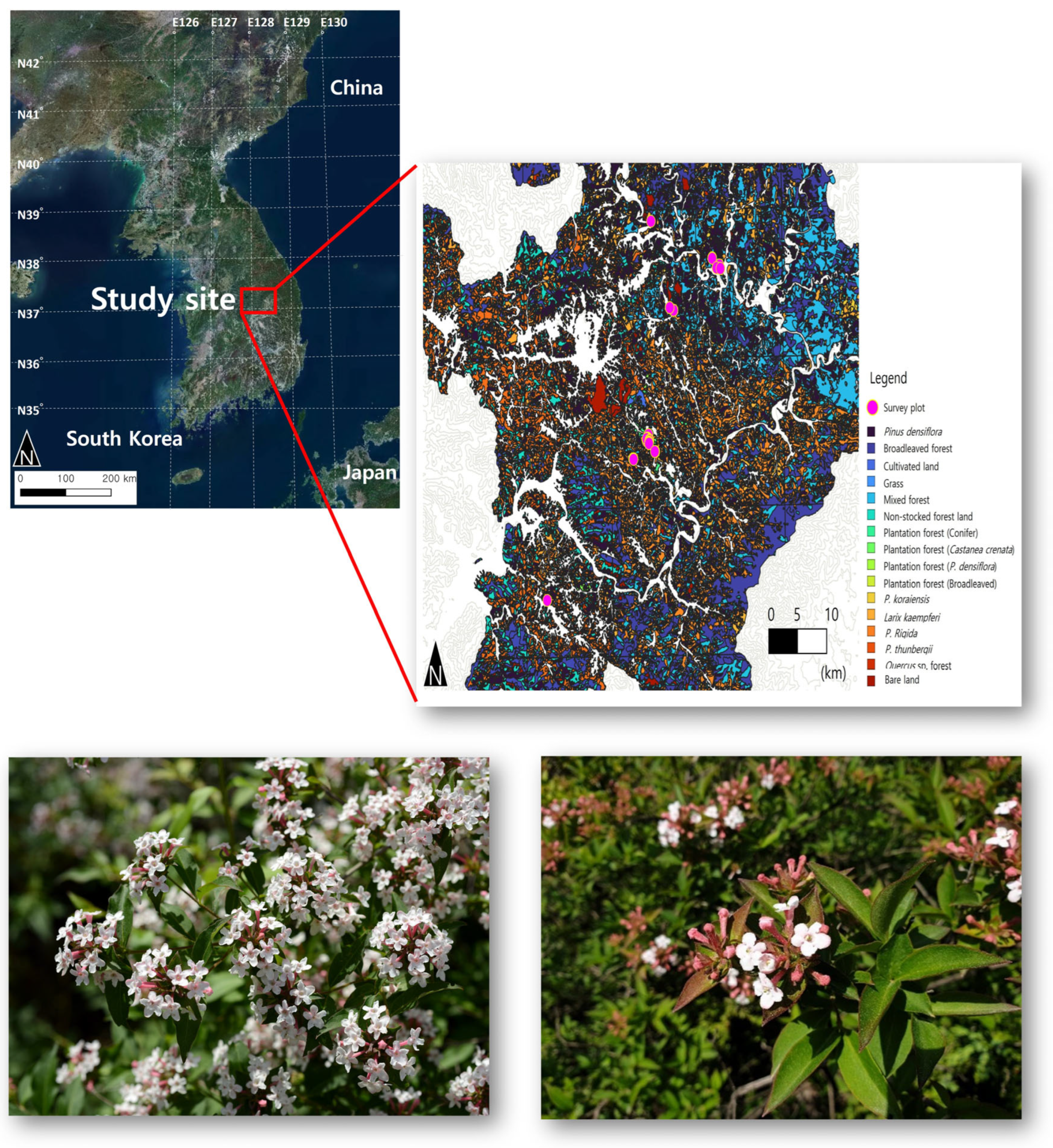
2.1. Study Site

The study site was located in the administrative districts of Jecheon-si, Danyang-gun, and Yeongwol-gun in South Korea, at a latitude of 36.9234–37.2408° and a longitude of 128.1546–128.4104°, with altitude ranges from 172 m to 421 m (Figure 1). Regarding the vegetation zone, the survey area comprises mixed conifer–broadleaf forests in the temperate central region, and the main vegetation communities are woody plant communities containing Quercus mongolicaLindera obtusiloba communities [23,24]. The study site included the Sobaeksan Mountain Range, which stretches in the northeast–southwest direction and has an altitude of over 1000 m. The study area is designated as a protected area by both the Korea Forest Service and the Ministry of Environment. The major mountains in the range include Mt. Wolaksan (1095 m), Mt. Soknisan (1058 m), and Mt. Joryeongsan (1026 m). The terrain surrounding the survey site has a highly variable altitude and contains numerous valleys and ridges. In particular, limestone is broadly distributed throughout the survey site, and the unique karst terrain provides habitats for various plants [11,25]. The climate in the Z. tyaihyonii habitats, based on data provided by the Korea Meteorological Administration, was as follows: mean temperature, 12.6 °C; maximum temperature, 17.9 °C; minimum temperature, 8.1 °C; relative humidity, 68.1%; annual precipitation, 1382.7 mm/yr; and mean wind speed, 2.2 m/s [26].

2.2. Survey Plot Placement and Survey Methods

We placed 36 survey plots (each 100 m2) in Z. tyaihyonii habitats in South Korea, placing one plot per habitat. The plots were distributed across the entire known range of the species, covering diverse environmental conditions within dry karst forest habitats. This sampling design ensured representative coverage across the species’ distribution. Considering the structure of the vegetation strata (tree, subtree, shrub, grass/herb), plant species, coverage, and abundance were recorded using the method of Braun-Blanquet [27]. The Braun-Blanquet method is mostly used in vegetation surveys in Asia and Europe and efficiently assesses community and species composition [28]. The survey period was from June 2021 to October 2023. Research reports published by the Korea National Arboretum and a fern atlas were used for identification. For scientific and common Korean names, the Korea Plant Names Index, provided by the Korea National Arboretum, was used [29,30,31,32,33,34,35].

2.3. Analysis

Jackknife analysis results for species richness were used to test whether an appropriate number of quadrats had been surveyed for vegetation analysis. Jackknife analysis is a method used for relatively small non-parametric samples, and it typically converges to the parameter faster than the estimate [36]. As a method of estimating the number of species, jackknife analysis can be used to estimate species richness by replicating the results of observed data. This method also enables estimating the cumulative species based on an optimal number of sampling points [36].
Cluster analysis was performed on the plant species observed at the 36 sampling points. The Sørensen method was used for the distance scale, and Ward’s method was used for cluster linkage [37]. Indicator species analysis was performed to determine the appropriate number of clusters for cluster analysis. The optimal number of groups was defined as the group count with the highest number of species with a significant p-value (p < 0.05) and the lowest mean p-value among these indicator species. The indicator values were tested using Monte Carlo simulation with 4999 iterations [37]. This number of iterations is commonly used in ecological studies to provide reliable p-value estimates while maintaining computational efficiency. The simulation tests the null hypothesis that species are randomly distributed among groups, thereby allowing for robust ecological interpretation of species–group associations [37]. The indicator values were calculated to select indicator species based on the determined group count (p < 0.05).
A multi-response permutation procedure (MRPP) analysis was used to test the cluster classification based on the heterogeneity in species composition between clusters. The distance was analyzed using the Sørensen method [37].
Important values were analyzed to label the clusters and verify species composition [38]. To this end, the relative coverage and relative frequency were calculated, and importance values were defined as (RC + RF)/2. As shown in Table 1, coverage and abundance were calculated as the median values at each level based on the Braun-Blanquet method [39]. The labels for each cluster were selected based on the species with the highest importance values.
Non-metric multidimensional scaling (NMDS) analysis was used to ascertain the distribution characteristics of survey plots within the clusters. Next, the two axes with the highest R2 (explanatory power) were selected, and the data were plotted in two dimensions [37]. NMDS uses a relative scale and is a useful method for analyzing non-parametric data with a high likelihood of relative discontinuity of ecosystems [37]. The main environmental factors used in the NMDS analysis were the topographic position index (TPI), the topographic wetness index (TWI), slope orientation, elevation, slope, organic matter, gravel fraction, pH, electrical conductance, exchangeable potassium, exchangeable calcium, exchangeable magnesium, exchangeable sodium, cation exchange capacity (CEC), exchangeable aluminum, species richness, evenness, species diversity, canopy openness, and light availability.
The TWI and TPI were extracted using a corrected digital elevation model (DEM). Since the raw DEM data could develop errors in the process of DEM generation, an error grid was extracted, and the ‘Fill’ tool was used to perform corrections using the surrounding grid, effectively removing errors during DEM construction. The TWI is defined as the measured amount of water flowing from the top of a local slope at a given point toward another given point; this means that the soil water content is lower when the local slope is steeper or the catchment area is smaller, and, conversely, the soil holds more water when the local slope is shallower or the catchment area is wider [40]. The TPI provides a quantitative measure of the shape of ridges and valleys using topographic characteristics, where a more negative index indicates a valley (concave) shape and a more positive index indicates a ridge (convex) shape [41].
The slope direction was first converted to an angle in radians, and then the cosine function was applied to obtain a value between −1 and 1. A number closer to 1 indicates a north-facing slope, and a number closer to −1 indicates a south-facing slope [42].
Species richness was defined as the number of species appearing within a survey plot, and species diversity was measured using the Shannon index [43]. For the TPI and TWI, data from the 36 survey plots were analyzed using options in the Arctoolbox of ArcGIS (ver. 10.8; Esri, Redlands, CA, USA).
The organic layer was removed to collect soil samples, and approximately 400 cc of soil was collected at a depth of 10–20 cm. The physicochemical properties of the soil were analyzed according to the categories shown in Table 2.
To measure light availability and canopy openness, photographs were taken from the center of each survey plot using a fisheye lens at a height of 1.2 m from the ground, keeping the camera horizontal and facing north. Photographs of the canopy were taken on overcast days at 3–6 pm to minimize errors due to sunlight [45]. The fisheye lens photographs were analyzed using Gap Light Analyzer (ver. 2.0; Figure 2).
To obtain an index to quantify the effects of human activity on Z. tyaihyonii, the habitat quality model in InVEST was used. Habitat quality can be used as an index to qualitatively assess biodiversity in a survey region [46,47,48]. Specifically, higher habitat quality indicates a region with superior biodiversity conservation, whereas lower habitat quality indicates inferior biodiversity conservation (Figure 3).
InVEST analysis is essentially based on land cover and uses data on the effects of threat factors on habitat quality, the radius of the effects of threat factors, and the sensitivity to threat factors of each subclassified factor indicated on the land cover map. Therefore, for this analysis, datasets were constructed to include habitat types, suitability, quality threat factors, quality sensitivity, and accessibility. Since habitat distance affects land-use types, corresponding weights must be applied to reflect its effects on habitat quality [49]. The scaling behavior of distance effects was categorized based on the properties of threat factors: linear scaling occurred when the threat factor was consistently affected by distance. At the same time, exponential scaling represented increasing effects of distance on the threat factor as distance increased (Table 3). The scaling behavior of the distance effects on the threat factors across habitat types and the distances was defined based on the criteria of the Korean National Institute of Ecology [50].
Using the habitat quality results based on InVEST modeling, a 2 km × 2 km grid was established around the survey site. This grid represented the minimum area of occupancy (AOO) of certain rare plants suggested by the IUCN. The habitat quality index of the survey site was calculated from the mean of pixels in the grid. The AOO suggested by the IUCN is defined as the minimum area required to ensure a suitable habitat for the survival of a given species population [51,52]; this was assumed to be an index of anthropogenic disturbance within areas with Z. tyaihyonii. ArcGIS (ver. 10.8; Esri, Redlands, CA, USA) was used for this analysis (Figure 4).
Zeta diversity was analyzed to identify trends in shared species contributing to biodiversity between habitats. Zeta diversity reflects trends in species turnover across all habitats or between habitats in each community. It measures species turnover depending on the species composition in the surveyed region in units of n survey plots. In other words, zeta diversity shows the number of species appearing in common in n survey plots and is expressed as the zeta order. Since zeta diversity means the ‘number of shared species,’ it is affected by species richness in the survey plots [53]. The zeta diversity ratio was analyzed to verify the interpretation of the decline in zeta diversity. The ζ-ratio shows the probability that a common species in n – 1 survey plots would also be present in the nth survey plot and is calculated using Equation (1) below.
ζ r a t i o = ζ n ζ n 1
where ζn is the number of species shared between n regions and ζn−1 is the number of species shared between n – 1 regions.
In this way, we aimed to interpret the spatial distribution patterns and the levels of species turnover between habitats. The analysis was conducted across four comparison conditions: all habitats, Com. 1 vs. Com. 2, Com. 1 vs. Com. 3, and Com. 2 vs. Com. 3.
Rare species contribute to the increase at lower orders, and as the order increases, the contribution of common species increases [53]. The ζ-ratio can exhibit patterns such as increasing, decreasing, and unimodal shapes [53]. In zeta diversity analysis, the fit of the positive exponential and power regression equations for the change in zeta diversity was tested to assess the process of species turnover between habitats. The significance of the fit was analyzed using Akaike’s Information Criterion (AIC) [54]. AIC is a criterion for assessing the fit of statistical models based on a balanced consideration of the model’s predictive power and complexity, effectively preventing overfitting by excluding extraneous variables [54]. The test result can be positive or negative, but relatively small values indicate a more reliable model [54]. Depending on the choice of the power function or exponential function, the interpretation of the process of ecological change differs. The power function model supports neutral theory, indicating that shared species appear repeatedly between habitats, while widespread species have a broad distribution. In other words, the appearance of a species is not viewed as the occupation of an ecological niche within the most optimal area. The exponential function model supports the stochastic and environmental filtering hypothesis. This hypothesis suggests that the heterogeneity in environmental factors causes different species distributions between habitats and that active species turnover can cause sudden changes in patterns of species composition in ecosystems [55,56]. ζ-diversity analysis was performed using the ‘zetadiv’ package in R Studio (https://posit.co/download/rstudio-desktop/) (R Foundation for Statistical Computing, Vienna, Austria) [57].
To examine statistically significant differences in environmental characteristics among the vegetation groups, a one-way analysis of variance (ANOVA) was performed, followed by Tukey’s HSD (Honestly Significant Difference) test for post hoc comparisons.

3. Results

3.1. Community Identification and Habitat Characterization

The species–area curve was analyzed to verify that an appropriate number of survey plots had been established (Figure 5). A total of 145 plant taxa were surveyed, and the slope and standard error of plant species richness approached 0 with an increasing number of survey plots, demonstrating that an appropriate number of survey plots had been established.
Conditions with two, three, and four clusters were compared in the analysis program to determine the optimal number of clusters. Several clusters (n = 5) were excluded from testing because they resulted in clusters with fewer than three locations, the minimum statistical unit. The highest number of indicator species and the lowest mean p-value were observed when the vegetation was grouped into three clusters, making this the optimal number of clusters for this study (Figure 6).
After cluster analysis (Figure 7), importance values were calculated by cluster. Combining the results of the cluster analysis and importance value calculation, the clusters were designated as Quercus dentataThuja orientalis communities (Com. 1), Fraxinus rhynchophyllaBuxus koreana communities (Com. 2), and Quercus dentataCarex humilis var. nana communities (Com. 3; Figure 7). MRPP analysis to test the heterogeneity in species composition between the communities revealed significant differences (p < 0.001) between all communities, demonstrating species composition heterogeneity between communities. Com. 1 and Com. 3 were characterized by Quercus spp., common woody plants in temperate broadleaf forests, with Q. dentata being the dominant upperstory vegetation [23]. While these two vegetation communities were mostly found at the edges of hiking trails in the mountains, Com. 2 was distributed around structures, such as transformers, and regions of ongoing construction work were observed close to its habitats. The F. rhyncophylla in Com. 2 grows in areas with relatively favorable water environments in temperate forests in South Korea [58].
When importance values were analyzed (Table 4), Z. tyaihyonii exhibited the lowest importance value in Com. 1, at 9.91, followed by 12.82 in Com. 2. It was most abundantly distributed in Com. 3, with an importance value of 24.86. Importance values in Com. 1 were in the order of Q. dentata (12.64) > Z. tyaihyonii (9.91) > T. orientalis (5.94) > C. humilis var. nana (4.19) > Juniperus rigida (3.99) > B. koreana (3.93). Importance values in Com. 2 were in the order of Z. tyaihyonii (12.82) > F. rhynchophylla (8.34) > B. koreana (6.90) > Carex lanceolata (3.83) > Thalictrum petaloideum (3.03). Importance values in Com. 3 were ranked as Z. tyaihyonii (24.86) > Q. dentata (10.20) > C. humilis var. nana (6.48) > F. rhynchophylla (3.42) > J. rigida (3.15) > Ulmus macrocarpa (2.42).
NMDS analysis was performed to determine the correlations with the environment by plotting the species composition of each community type in two-dimensional space (Figure 8). Axes 1 and 2 had the highest R2 values of 0.475 and 0.168, respectively, and the combined R2 was 0.643. Com. 1 and Com. 3 distributions were relatively close, but Com. 2 showed a somewhat distinct distribution, suggesting species composition differences. In particular, the species compositions of Com. 2 and Com. 3 were highly heterogeneous. When the environmental factors were analyzed by community type, calcium content, and species richness, correlations were observed.
An indicator species analysis was performed to identify the plant species that affect the composition of heterogeneous species in each community type (Table 5).
Com. 1, Com. 2, and Com. 3 contained seven, three, and seven indicator species, respectively. The indicator species in Com. 1 included Q. dentata (53.9), Spiraea chinensis (47.6), and Quercus variabilis (46.2). The indicator plant species that differentiated Com. 2 were B. koreana (48.0), Z. tyaihyunii (40.3), C. lanceolata (40.0), and Neillia uyekii (40.0). The indicator species in Com. 3 included Crepidiastrum sonchifolium (62.5), C. humilis var. nana (51.9), and Euonymus alatus (47.6).
Table 6 presents the findings from the analysis of environmental factors by the Z. tyaihyonii community. Environmental factors were classified into geographic and vegetational factors, species diversity, and soil properties. ANOVA was performed to compare each factor between community types. The altitude was relatively low at 200–250 m, and the slope was shallow at 6–8°. Due to the flat terrain, the TPI was negative in all community types, and due to the increase in the catchment area, the TWI was around 8–9. Northness was negative in all community types, meaning that most slopes were south-facing. In Com. 1, northness was –0.72 ± 0.10, implying that these communities were located on south-facing slopes more than the other community types. South-facing slopes have more abundant light availability than other slope directions, resulting in dry, warm environments [59,60,61,62]. Canopy openness was around 45%–54%, and light availability was ample, with transmitted light of 14.87–18.29 mole·m−2·d−1. Significant differences between community types were not observed for the seven geographic and vegetational factors (p > 0.05).
Regarding soil properties, organic matter was approximately 17%–18%, and the gravel fraction was 43%–50%, resulting in a dry soil environment amenable to water drainage. Among the exchangeable cations, calcium concentrations showed a significant difference between community types (p < 0.05), with higher concentrations in Com. 2.
Among species diversity-related factors, species richness, diversity (Shannon index), and evenness showed significant differences between community types (p < 0.05), with all factors being lower in Com. 2.
Habitat quality was assessed to investigate the level of disturbance due to human activities (Figure 9). The mean habitat quality across all habitats was 0.5562 ± 0.0294. Considering community type, the habitat quality was 0.5800 ± 0.0585 in Com. 1, 0.4633 ± 0.0309 in Com. 2, and 0.6919 ± 0.0357 in Com. 3. Com. 2 showed the lowest habitat quality, and the differences in habitat quality between community types were significant (p < 0.01). Limestone mining and the installation of human structures were observed near habitats in Com. 2 (Figure 10).

3.2. Zeta Diversity and Species Turnover

Analysis of the zeta diversity decline graph (Figure 11a) showed that Com. 1 vs. Com. 3 exhibited a more gradual decline in zeta diversity relative to the other comparisons, suggesting a higher degree of shared species between these habitats. In essence, this underscores the relative persistence of habitat connectivity. Conversely, in all comparisons that included Com. 2, zeta diversity declined sharply from zeta order 2 and converged to 1 from zeta order 7, showing almost identical values.
Analysis of the zeta ratio (Figure 11b) demonstrated that all comparison groups approached a zeta ratio of 1 with increasing zeta order. However, except for Com. 1 vs. Com. 3, all other comparison groups showed a rapidly oscillating zeta ratio within the zeta order range of 8–12. The Com. 1 vs. Com. 3 group showed a relatively stable increase in the zeta ratio.
To elucidate the hypotheses that underpin different ecological change processes, exponential and power function models were evaluated for each comparison group, and the AIC of each function was analyzed (Figure 11c,d). The AIC was lower for the power function in all comparison groups, suggesting it as the appropriate model for interpreting ecological change processes in this study and supporting the niche process theories. In the comparison of zeta diversity decline among communities, the analysis of Com. 2 vs. Com. 3 supported the stochastic hypothesis.

4. Discussion

4.1. Community Identification and Habitat Characterization

This study focused on Z. tyaihyonii habitats with different species compositions. To this end, we analyzed the correlations between environmental factors and different Z. tyaihyonii community types and identified communities to prioritize for conservation; this was performed to provide data to support policymaking for the efficient maintenance of biodiversity. The purpose of analyzing species composition and environmental factors of Z. tyaihyonii was to classify vegetation communities and identify the environmental and natural factors. Even in the same region, evenly inhabited by a given species, differences in the surrounding environment can produce different conditions for maintaining or promoting a population, and identifying these effects is an important task for conservation biology [63,64,65].
The identified communities were broadly classified into three types. For Com. 1 and Com. 3, both community types included Q. dentata in the subtree layer, resulting in similar canopies, whereas the canopy in Com. 2 comprised F. rhynchophylla. T. orientalis in Com. 1 and B. koreana in Com. 2 are commonly distributed in limestone regions in South Korea [10] and have ecological niches and habitat environments similar to those of Z. tyaihyonii, which is the species of interest in this study. Although the Fraxinus genus tends to grow in valleys or other moist environments, it is resistant to dry conditions [66]. Our study area was rich in limestone, resulting in mildly alkaline soil. These soil properties interfere with the growth of woody plants and negatively affect subsequent succession and regeneration [67]. Therefore, the development of woody plant layers across all Z. tyaihyonii community types is expected to decline over time.
B. koreana and T. orientalis, the predominant shrub species in these communities, are calcicoles mainly distributed in regions characteristic of the study site. Since they have a similar ecological niche to Z. tyaihyonii, they were considered spatial competitors. Meanwhile, plants such as C. humilis var. nana, C. lanceolata, Securinega suffruticosa, and E. alatus are mostly found in dry vegetation with ample light availability [68,69].
In regions with elevated soil calcium levels and a high gravel fraction, intensified water stress and alkaline soil conditions make growth difficult for most plants, ultimately leading to low species richness [70]. The soil in limestone regions is rich in calcium and carbonates, resulting in an alkaline pH. Additionally, its single-grain structure contributes to the dry physical properties of the soil [71,72]. The pH was 7.6–7.8, indicating an alkaline soil environment attributed to the high calcium and carbonate concentrations [61,63]. When these minute soil differences persist over an extended period, they could develop a unique ecosystem structure shaped by adaptation to this environment [71,72]; this is supported by the low evenness observed in the current study, suggesting the potential presence of plants unique to Com. 2 that are absent in the other community types. Evenness reflects the degree to which plant species are evenly distributed within a community and tends to decrease when a few species dominate the ecological niche, thereby limiting the presence of others [73,74]. In our study, the observed statistically significant differences in evenness among the community groups suggest that evenness may serve as an important ecological indicator for predicting future changes in species composition and community structure.
Although Z. tyaihyonii was found across multiple habitat groups, the species was statistically significant as an indicator species for Com. 2 (indicator value = 40.3, p = 0.0002). We acknowledge that Com. 2 deserves particular attention. In addition, the indicator species in Com. 2 were all calcicoles, with B. koreana and N. uyekii being especially strongly calcicolous plants [11]. Indicator values were calculated, and plant species with significant differences (p < 0.05) were selected. In other words, these species differentiate one community type from the others [75]. In addition, indicator species are plant species that need focused ecosystem conservation and management [75,76].
Importantly, this group also showed the lowest habitat quality among the classified clusters, suggesting it may represent both a critical and vulnerable habitat. Therefore, conservation efforts should prioritize Com. 2 while also maintaining broader protection strategies across the entire distribution range of the species.
However, the Z. tyaihyonii habitats in the present study were affected by habitat fragmentation and active edge effects due to their location on the periphery of forests; this increases the likelihood of invasion by external species [77,78]. Although Aster pilosus, an invasive plant in South Korea, was detected in Community 1, its importance value was relatively low (0.130), indicating that it does not currently pose a significant threat to Z. tyaihyonii. Nevertheless, continued habitat fragmentation may increase opportunities for invasive species to establish. Thus, one limitation of the current study was its short duration, and further studies will be needed for long-term monitoring of biodiversity trends.
In the InVEST model analysis, habitat quality in the current study was mostly moderate; this suggests that the habitats are at a critical juncture between biodiversity preservation and degradation, with future outcomes determined by the extent of disturbance they experience. Habitat quality in a thriving forest ecosystem is 0.9 or higher, whereas in a region with severe ecological disturbance, such as an industrial zone, it is approximately 0.2–0.3 [79]. This moderate habitat quality will rapidly deteriorate if human activities, such as road construction or indiscriminate forest clearing, continue, as these actions significantly accelerate habitat fragmentation and ecological degradation [80,81]. Rapid urbanization causes habitat loss and affects species distribution through fragmentation, ultimately diminishing the resilience and stability of communities [82,83]. In addition, ecologically disruptive invasive species alter the habitats of native species, resulting in frequent species turnover and an unstable ecosystem structure [84].

4.2. Zeta Diversity and Species Turnover

Addressing the trends in Com. 2, which showed the poorest habitat quality, requires continuous monitoring and prioritizing conservation activities in these communities. Rapid species turnover featured prominently in comparison groups that included Com. 2, owing to the rapidly declining zeta diversity and a zeta ratio that exhibited an oscillating pattern at certain zeta orders. These trends support the idea of ecosystem instability.
In all groups, the number of shared species was almost consistent with increasing zeta order (number of habitats), showing the homogeneity in the habitat environments. However, rapid oscillations in the zeta ratio at specific zeta orders indicate irregular spatial patterns [85]; this implies that shared species show large ecological variance at the spatial scale of certain habitats, indicating that these habitats are undergoing ecological succession, which is thought to be due to the irregularity of the ecosystem structure due to frequent disturbances caused by human activity. When the zeta ratio rapidly decreases (i.e., when the number of shared species between habitats decreases), it suggests that strong environmental restrictions (rivers, mountains, etc.) demarcate clear habitat boundaries [85]. However, in our results, the zeta ratio converged to 1 with increasing zeta order, suggesting that the habitats have similar environmental conditions. Specifically, the habitat environments in the present study site are characterized by lime-rich soil conditions in karst terrain, with low altitude and shallow slopes, representing a relatively even ecological environment overall [12,19]. However, the reason why species turnover in each community showed irregular oscillating patterns in certain regions (zeta order 8–12) is thought to be due to edge effects resulting from hiking trail construction at the forest periphery, human-made structures, and habitat fragmentation. These act as drivers of frequent species turnover in certain regions of heavy disturbance. These findings were supported by the NMDS analysis between community types, where species richness was identified as a factor significantly affecting species composition.
Based on the zeta diversity analysis, the power function model was the best fit, supporting the niche process theory of ecological change [53,57]. Support for the power function model across all Z. tyaihyonii habitats is thought to show the presence of spatial autocorrelation due to the target species’ preference for lime-rich soil.
However, as confirmed through field surveys and the habitat quality assessment, Com. 2 exhibited severe habitat fragmentation caused by nearby anthropogenic disturbances, and this threat continues to intensify. In particular, the exponential model provided a better fit for the Com. 2 vs. Com. 3 comparison, supporting the hypothesis of stochastic processes and environmental filtering. Com. 2 is located in areas with active human activities, such as mining and construction, which have generated distinct environmental conditions compared to Com. 3. These environmental differences appear to drive species compositional divergence, as demonstrated by NMDS analysis, which showed a clear spatial separation in species composition between the two communities.
In fragmented ecosystems, species often utilize different resources or microhabitats to avoid direct competition [56]. Such niche differentiation promotes species heterogeneity, leading, over time, to the emergence of spatially distinct, patch-like habitats [86,87]. Habitat fragmentation further facilitates the invasion of opportunistic species due to altered environmental gradients, increasing interspecific competition. This may accelerate niche partitioning as species adapt spatially to minimize overlap and competition [88]. Ultimately, these dynamics contribute to heightened species turnover across fragmented habitats.

4.3. Conservation Strategy and Direction

This study aimed to investigate Z. tyaihyonii, an endemic Korean plant, using a conservation biology and biodiversity analysis approach to select populations to prioritize conservation, thereby providing directions for efficient conservation. Based on the results, Com. 2 regions, characterized by the indicator species B. koreana, C. lanceolata, and N. uyekii, should be continuously monitored as conservation regions. When differences in environmental factors between the community types were analyzed, species richness and soil calcium concentrations significantly differed, with Com. 2 showing clear differences from other community types in comparisons of habitat quality and zeta diversity. In terms of ecological health, although the habitats showed moderate habitat quality, if anthropogenic disturbances increase in the future, habitat quality could decline further, and species turnover caused by habitat fragmentation could lead to long-term instability of ecosystem structure. As evidence of this state, zeta diversity rapidly declined, and the zeta ratio showed an oscillating pattern in certain zeta orders.
Analyzing biodiversity health takes a long time. Predictions of biodiversity changes are too short-term for understanding ecosystems, and firmly declaring the causes of long-term population survival based on partial interpretations is challenging. However, persistent or repeated human activity inevitably leads to population decline due to habitat fragmentation. Therefore, predicting the distribution of certain populations is essential for long-term conservation activities.
Species distribution modeling needs to be performed at the level of landscape ecology units based on direct field monitoring of habitats. Previously, predictions relying on single models were fraught with significant uncertainty. However, recent advances in deep and machine learning techniques have broadened their application to forest ecology; this has led to active efforts to utilize ensemble models, which combine multiple models, to enhance the efficiency and precision of biodiversity conservation efforts. These efforts aim to address climate change by improving the accuracy of predictive techniques. Predicting changes in habitat distribution and identifying threat factors under the new climate change scenarios outlined in the IPCC’s latest adaptation plan is a critical priority. Establishing basic data through field surveys is paramount to improving modeling accuracy. Thus, interpreting ecological information requires integrating insights from landscape ecology and field monitoring. This combination is crucial for developing efficient conservation strategies supported by robust scientific evidence.
Having identified the threat factors for Z. tyaihyonii in this study, the critical focus lies in the policy options formulated and presented to conservation policymakers. The first is ‘regulating human activities by actively designating protected areas,’ and the second is ‘community sharing of conservation activities for rare and endemic plants.’
The biggest issue for biodiversity recently is the balance between ecosystem use and conservation. The commercial value of Z. tyaihyonii and the limestone obtained from the rocks in Z. tyaihyonii habitats are essential for human use. As the concept of Nature’s Contribution to People (NCP) has expanded, biodiversity conservation activities are affecting the affluent lifestyles of humans in terms of ecosystem services. To this end, increasing attention is being drawn to the importance of balancing ongoing conservation efforts with the use of biological resources [89,90]. Regulations on development in certain regions are needed to achieve sustainable biological resources and improve the value of environmental resources. Urbanization due to humans can rapidly isolate and alter the structure and abiotic limiting factors in certain ecosystems, and ecological niches become even more prominent in endemic plants in specific relict populations [91]. Conserving these resources, passing them on to future generations, and generating value from sustainable forest resources are responsibilities that rest with humanity. In the future, finding a balance between human use and conservation of biological resources by utilizing research results and policies to select protected regions will be necessary.
The post-2020 GBF of the CBD highlights the need to extend beyond population ecology approaches to the restoration and conservation of habitat environments to achieve efficient species conservation [3]. Expanding protected areas has been set as a practical target, and each country has been advised to implement biodiversity conservation policies to achieve this. To prepare efficient conservation strategies for domestic endangered species, we will need to continually survey population distributions and fluctuations and analyze nearby habitat environments to prepare multifaceted conservation measures.
Ecological conservation is not solely the domain of government organizations; it requires collaboration with local communities. However, this will require additional research on the value of certain plant habitats within a region, functional aspects, and the benefits of biodiversity conservation for humans [92].
To this end, quantifying the roles of ecosystems by analyzing the ecological functions of the habitats of certain species is critical. This research will provide foundational data to effectively inform the public of the validity of the conservation of species [93].
Based on scientific evidence, governments should encourage residents to voluntarily engage in conservation activities through education and publicity. Biodiversity conservation for endemic plants is limited by reliance solely on protection policies and management at the government level. True conservation outcomes are only achieved when coupled with community members’ interest and proactive participation. In particular, one reason for persistent, indiscriminate development is the public’s lack of awareness of endemic plants’ ecological and cultural value. This lack of awareness is due to insufficient education and publicity of biodiversity, which ultimately causes residents to overlook the presence and importance of endemic plants in their environments; this leads to indiscriminate development and habitat destruction. Therefore, to achieve effective biodiversity conservation, systematic education programs and publicity campaigns must be conducted at the community level to inform residents of the need to protect endemic plants. Creating a local environment where residents understand the balance between development and conservation and actively participate in protection activities paves the way for sustainable biodiversity conservation (Figure 12).

5. Conclusions

This study addressed three key objectives: (1) to analyze the vegetation structure of Z. tyaihyonii habitats, (2) to explore the relationships between environmental factors and biodiversity patterns, and (3) to support conservation planning.
First, the community classification revealed three distinct vegetation types associated with Z. tyaihyonii, with species composition varying significantly among them. Com. 2, in particular, exhibited lower species richness and habitat quality, highlighting its vulnerability. Second, the analysis of environmental factors, including soil calcium and species evenness, identified ecological constraints that may limit the species’ distribution and regeneration potential—especially under alkaline, dry soil conditions common in karst terrain. Third, zeta diversity modeling provided insights into habitat connectivity and species turnover. While most communities showed gradual turnover consistent with niche-based processes, the comparison between Community 2 and Community 3 supported stochastic and environmental filtering theory, indicating fragmentation and ecological instability.
Collectively, these findings indicate that Z. tyaihyonii functions as a relict species persisting in fragmented and geologically specialized habitats, where its ecological niche is narrowly defined and easily disrupted. Given the growing pressures from mining, development, and habitat fragmentation, the species is at increased risk of local extinction.
Although this study employed a strictly ecological framework, the results underscore the need for integrating socio-economic and cultural values into conservation planning. The conservation of endemic plants like Z. tyaihyonii must not be limited to protecting habitats alone but should also account for their broader ecosystem services and roles in cultural identity. Future strategies should therefore adopt a holistic, interdisciplinary approach that incorporates ecological data, landscape-level threats, and human dimensions of conservation. Continued field monitoring and modeling will be essential to refine these strategies and to ensure the long-term sustainability of endemic species in rapidly changing landscapes.
In conclusion, this study not only supports the conservation of Z. tyaihyonii but also provides a practical road map for preserving other endemic Korean plant species facing comparable conservation threats.

Author Contributions

Conceptualization, B.-J.P. and K.-I.C.; software, B.-J.P.; formal analysis, B.-J.P. and K.-I.C.; investigation, B.-J.P., T.-I.H. and K.-I.C.; writing—original draft, B.-J.P. and T.-I.H.; writing—review and editing, K.-I.C.; data curation, B.-J.P.; visualization, B.-J.P. All authors have read and agreed to the published version of the manuscript.

Funding

This research was funded by the Baekdudaegan National Arboretum (2023-01-01-02) and the National Institute of Ecology (Project No. NIE-B-2025-03).

Data Availability Statement

The datasets used and/or analyzed during the current study are available from the corresponding author upon reasonable request.

Acknowledgments

This research was conducted as part of Baekdudaegan Natioanal Arboretum’s research project, ‘Research on the Target Plant Species in Baekdudaegan for Conservation Status Assessments and Strategies (2023-01-01-02)’, the National Institution of Ecology’s research project, ‘Development of Policy Decision Support System Base on Ecosystem Services Assessment (Project No. NIE-B-2024-03)’, and the Korea Environmental Industry & Technology Institute project, ‘Development of decision support integrated impact assessment model for climate change, adaptation: ecosystem (Project No. 2022003570001)’ in Republic of Korea.

Conflicts of Interest

The authors declare no conflicts of interest.

References

  1. Convention on Biological Diversity. Available online: https://www.cbd.int/gbf (accessed on 29 January 2024).
  2. Park, B.J.; Han, S.K.; Park, S.H.; Cheon, K.; Che, S.H.; Heo, T.I. Correlation between Vegetation Structure and Environmental Factors of Dracocephalum argunense Habitats in South Korea. J. Korean Soc. For. Sci. 2024, 113, 271–281. [Google Scholar]
  3. Koo, K.A.; Park, S.U. A Review of Ecological Niche Theory from the Early 1000s to the Present. Korean J. Environ. Ecol. 2021, 35, 316–335. [Google Scholar] [CrossRef]
  4. The Red List of Threatened Species. Available online: https://www.iucnredlist.org/en (accessed on 11 March 2025).
  5. Thompson, J.D.; Lavergne, S.; Affre, L.; Gaudeul, M.; Debussche, M. Ecological differentiation of Mediterranean endemic plants. Taxon 2005, 54, 967–976. [Google Scholar] [CrossRef]
  6. Aikens, M.L.; Roach, D.A. Population dynamics in central and edge populations of a narrowly endemic plant. Ecol. 2014, 95, 850–1860. [Google Scholar] [CrossRef]
  7. Chae, H.H.; Kim, Y.C.; Son, S.W. Korean and Worldwide Research Trends on Rare Plant and Endemic Plant in Korea. Korean J. Environ. Ecol. 2022, 36, 257–276. [Google Scholar] [CrossRef]
  8. Chung, G.Y.; Jang, H.D.; Chan, K.S.; Choi, H.J.; Kim, Y.S.; Kim, H.J.; Son, D.C. A checklist of endemic plants on the Korean Peninsula II. Korean J. Plant Taxon. 2023, 53, 79–101. [Google Scholar] [CrossRef]
  9. Jeong, J.H.; Kim, K.S.; Lee, C.H.; Kim, Z.S. Genetic diversity and spatial structure in populations of Abelia tyaihyoni. J. Korean Soc. For. Sci. 2007, 96, 667–675. [Google Scholar]
  10. Chung, G.Y.; Chang, K.S.; Chung, J.M.; Choi, H.J.; Paik, W.G.; Hyun, J.O. checklist of endemic plants on the Korean Peninsula. Korean J. Plant Taxon. 2017, 47, 264–288. [Google Scholar] [CrossRef]
  11. Kim, J.H.; Nam, G.H.; Lee, S.B.; Shin, S.G.; Kim, J.S. A checklist of vascular plants in limestone areas on the Korean Peninsula. Korean J. Plant Taxon. 2021, 51, 250–293. [Google Scholar] [CrossRef]
  12. Kim, J.D.; Lee, H.J.; Lee, D.H.; Byeon, J.G.; Park, B.J.; Heo, T.I. Characteristics of environmental factors and vegetation Community of Zabelia tyaihyonii (Nakai) Hisauti & H.Hara among the target plant species for conservation in Baekdudaegan. J. Korean Soc. For. Sci. 2022, 111, 201–223. [Google Scholar]
  13. Korea National Arboretum. Rare plants in Korea; Sumeungil: Seoul, Republic of Korea, 2012; pp. 1–412. ISBN 978899745038196480. [Google Scholar]
  14. Chae, H.H.; Kim, Y.C.; Hong, B.R.; Lee, K.S.; Son, S. Distributional status and evaluation of species traits a Korean endemic plant of Zabelia tyaihyonii (Nakai) Hisauti and Hara (Caprifoliaceae). J. Asia-Pac. Biodivers 2023, 16, 372–383. [Google Scholar] [CrossRef]
  15. Cho, S.Y.; Yim, G.J.; Lee, J.Y.; Ji, S.W. A Review of the Regeneration Models using a Closed Stone Quarry Area through Domestic and Overseas Cases. KSMER 2021, 58, 237–248. [Google Scholar] [CrossRef]
  16. Habel, J.C.; Assmann, T.; Schmitt, T.; Avise, J.C. Relict Species: From Past to Future; Springer: Berlin, Germany, 2010; pp. 1–5. ISBN 9783540921608. [Google Scholar]
  17. Grandcolas, P.; Nattier, R.; Trewick, S. Relict species: A relict concept? Trends Ecol. Evol. 2014, 29, 655–663. [Google Scholar] [CrossRef]
  18. Legg, S. IPCC, 2021: Climate Change 2021-The Physical Science Basis. Interaction 2021, 49, 44–45. [Google Scholar]
  19. Kim, K.A.; Jang, S.K.; Cheon, K.S.; Seo, W.B.; Yoo, K.O. Environmental and ecological characteristics of habitats of Abelia tyaihyoni Nakai. Korean J. Plant Taxon. 2010, 40, 135–144. [Google Scholar] [CrossRef]
  20. Ghimire, B.; Suh, G.U.; Lee, C.H.; Heo, K.; Jeong, M.J. Embryological studies on Abelia tyaihyoni Nakai (Caprifoliaceae). Flora 2018, 242, 79–88. [Google Scholar] [CrossRef]
  21. Lee, W.; Youn, J.S.; Kim, S.C.; Pak, J.H. The complete chloroplast genome sequence of limestone endemic, Zabelia tyaihyoni (Caprifoliaceae), in Korea. mtDNA Part B 2020, 5, 1947–1948. [Google Scholar] [CrossRef]
  22. Choi, I.S.; Han, E.K.; Wojciechowski, M.F.; Heo, T.I.; Park, J.S.; Yang, J.C.; Gantsetseg, A.; Cheon, K.S.; Tamaki, I.; Lee, J.H. The genetic structure and demographic history of Zabelia tyaihyonii, endemic to Korean limestone karst forests, based on genome-wide SNP markers. Ecol. Evol. 2023, 13, e10252. [Google Scholar] [CrossRef]
  23. Kim, J.W.; Lee, Y.G. Classification and Assessment of Plant Communities; World Science: Seoul, Republic of Korea, 2006; pp. 33–60. ISBN 9788958810605. [Google Scholar]
  24. Korea National Arboretum. 2020. Forest of Korea(IV) Biogeography of Korea: Flora and Vegetation; Sumeungil: Seoul, Republic of Korea, 2020; pp. 42–79. ISBN 9791190509497. [Google Scholar]
  25. Nam, G.H.; Kim, J.H.; Kim, Y.C.; Kim, K.S.; Lee, B.Y. Floristic Study of County Pyeong-chang and Yeong-wol including Limestone Regions (Prov. Gangwon-do) from Korea. Korean J. Environ. Ecol. 2012, 26, 11–38. [Google Scholar]
  26. Climate Data in South Korea. Available online: http://www.kma.go.kr (accessed on 20 January 2025).
  27. Braun-Blanquet, J. Pflanzensoziologie: Grundzüge Der Vegetationskunde; Springer: Wien, Austria, 1964; pp. 17–205. ISBN 9783709181119. [Google Scholar]
  28. Ivanova, N. Global Overview of the Application of the Braun-Blanquet Approach in Research. Forests 2024, 15, 937. [Google Scholar] [CrossRef]
  29. Korea Fern Society. Ferns and Fern Allies of Korea; Geobook: Seoul, Republic of Korea, 2005; pp. 1–399. ISBN 9788995504925. [Google Scholar]
  30. Korea National Arboretum. Rare Plants Data Book in Korea; Geobook: Seoul, Republic of Korea, 2008; pp. 1–332. ISBN 9788991458352. [Google Scholar]
  31. Korea National Arboretum. Invasive Alien Plant Impact on Forest; Sumeungil: Seoul, Republic of Korea, 2015; pp. 1–280. ISBN 9791187031185. [Google Scholar]
  32. Cho, Y.H.; Kim, J.H.; Park, S.H. Grasses and Sedges in South Korea; Geobook: Seoul, Republic of Korea, 2016; pp. 1–528. ISBN 9788994242422. [Google Scholar]
  33. Korea National Arboretum. Checklist of Vascular Plants in Korea; Samsung edCOM: Seoul, Republic of Korea, 2017; pp. 1–1000. ISBN 9791188720125. [Google Scholar]
  34. Korea National Arboretum. Native & 100 Cultivar Caprifoliaceae; Blue Sensation: Seoul, Republic of Korea, 2022; pp. 1–147. ISBN 9791192743097. [Google Scholar]
  35. Knowledge system of National species in Korea. Available online: http://www.nature.go.kr/kpni (accessed on 3 January 2025).
  36. Kang, C. A study of the jackknife estimate. J. Ind. Sci. Technol. 2002, 34, 325–331. [Google Scholar]
  37. McCune, B.; Grace, J.B. Analysis of Ecologcial Communities; MjM Software Design: Gleneden Beach, OR, USA, 2002; pp. 179–204. ISBN 9780972129008. [Google Scholar]
  38. Curtis, J.T.; McIntosh, R.P. An upland forest continuum in the prairie-forest border region of Wisconsin. Ecology 1951, 32, 476–496. [Google Scholar] [CrossRef]
  39. Park, B.J.; Heo, T.I.; Cheon, K.I. Analyzing Generalist Plant Species Using Topographic Characteristics of Picea jezoensis (Siebold & Zucc.) Carrière Forests in East Asia: From China (Mt. Changbai) to South Korea. Int. J. Plant Biol. 2024, 15, 320–339. [Google Scholar]
  40. Petroselli, A.; Vessella, F.; Lucia, C.; Piovesan, G.; Schirone, B. Ecological behavior of Quercus suber and Quercus ilex inferred by topographic wetness index (TWI). Trees 2013, 27, 1201–1215. [Google Scholar] [CrossRef]
  41. Zwolinski, Z.; Stefańska, E. Relevance of moving window size in landform classification by TPI. Geomorphometry Geosci. 2015, 2015, 273–277. [Google Scholar]
  42. McCune, B.; Keon, D. Equations for potential annual direct incident radiation and heat load. J. Veg. Sci. 2002, 13, 603–606. [Google Scholar] [CrossRef]
  43. Shannon, C.E. A mathematical theory of communication. Bell Syst. Tech. J. 1948, 27, 379–423. [Google Scholar] [CrossRef]
  44. Klute, A. Methods of Soil Analysis Part 1 Physical and Mineralogical Methods; American Society of Agronomy: Madison, WI, USA, 1986; pp. 383–411. ISBN 9780891180883. [Google Scholar]
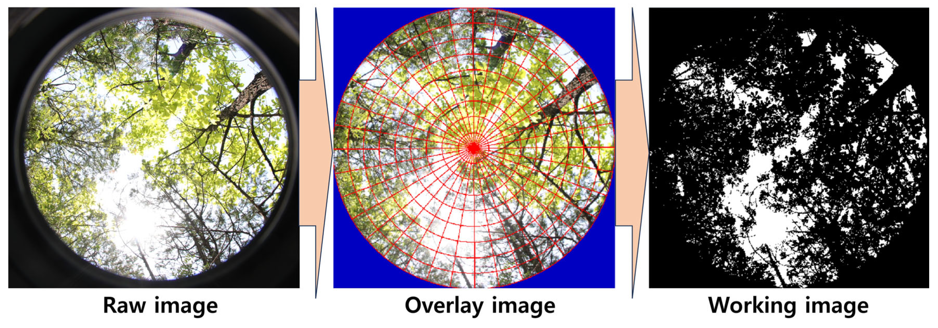
  45. Beckschäfer, P.; Seidel, D.; Kleinn, C.; Xu, J. On the exposure of hemispherical photographs in forests. Ifor.-Biogeosci. For. 2013, 6, 228. [Google Scholar] [CrossRef]
  46. Nelson, E.; Mendoza, G.; Regetz, J.; Polasky, S.; Tallis, H.; Cameron, D.; Chan, K.M.; Daily, G.C.; Goldstein, J.; Kareiva, P.M.; et al. Modeling multiple ecosystem services, biodiversity conservation, commodity production, and tradeoffs at landscape scales. Front. Ecol. Environ. 2009, 7, 4–11. [Google Scholar] [CrossRef]
  47. Gao, J.; Li, F.; Gao, H.; Zhou, C.; Zhang, X. The impact of land-use change on water-related ecosystem services: A study of the Guishui River Basin, Beijing, China. J. Clean. Prod. 2017, 163, 148–155. [Google Scholar] [CrossRef]
  48. Jang, J.E.; Kwon, H.Y.; Shing, H.S.; Lee, S.C.; Yu, B.H.; Jang, J.; Choi, S.H. Habitat quality analysis and evaluation of InVEST model using QGIS: Conducted in 21 national parks of Korea. Korean J. Environ. Ecol. 2022, 36, 102–111. [Google Scholar] [CrossRef]
  49. Nellemann, C.; Vistnes, I.; Jordhøy, P.; Strand, O. Winter distribution of wild reindeer in relation to power lines, roads and resorts. Biol. Conserv. 2001, 101, 351–360. [Google Scholar] [CrossRef]
  50. National Institute of Ecology. The Manual of Assessment Map of Ecosystem Service; Design Crepas: Seoul, Republic of Korea, 2022; pp. 54–61. ISBN 9791166981463. [Google Scholar]
  51. Kumar, P. Tools for Measuring modelling, and Valuing Ecosystem Services; IUCN: Gland, Switzerland, 2018; pp. 1–293. ISBN 9782831718965. [Google Scholar]
  52. National Institute of Biological Resources. Guidelines for Using the IUCN Red List Categories and Criteria (Korean Version); Doohyun Publishing: Seoul, Republic of Korea, 2015; pp. 57–71. ISBN 9788968112485. [Google Scholar]
  53. McGeoch, M.A.; Latombe, M.; Andrew, N.R.; Nakagawa, S.; Nipperess, D.A.; Roigé, M.; Marzinelli, E.M.; Campbell, A.H.; Vergés, A.; Thomas, T.; et al. Measuring continuous compositional change using decline and decay in zeta diversity. Ecology 2019, 100, e02832. [Google Scholar] [CrossRef] [PubMed]
  54. Akaike, H. A new look at the statistical model identification. IEEE Trans. Autom. Control 1974, 19, 716–723. [Google Scholar] [CrossRef]
  55. Gaston, K.J.; He, F. The distribution of species range size: A stochastic process. Proc. R. Soc. Lond. B 2002, 269, 1079–1086. [Google Scholar] [CrossRef]
  56. Zuppinger-Dingley, D.; Schmid, B.; Petermann, J.S.; Yadav, V.; De Deyn, G.B.; Flynn, D.F. Selection for niche differentiation in plant communities increases biodiversity effects. Nature 2014, 515, 108–111. [Google Scholar] [CrossRef]
  57. Latombe, G.; McGeoch, M.A.; Nipperess, D.A.; Hui, C. zetadiv: An R package for computing compositional change across multiple sites, assemblages or cases. bioRxiv. [CrossRef]
  58. Park, B.J.; Kim, J.J.; Byeon, J.G.; Cheon, K.; Joo, S.H.; Lee, Y.G. The classification of forest community and character of stand structure in Mt. Myeonbong: Focused on research forest in Kyungpook National University, Cheongsong. J. Korean Soc. For. Sci. 2016, 105, 391–400. [Google Scholar] [CrossRef]
  59. Weltzin, J.F.; Loik, M.E.; Schwinning, S.; Williams, D.G.; Fay, P.A.; Haddad, B.M.; Harte, J.; Huxman, T.E.; Knapp, A.K.; Lin, G.H.; et al. Assessing the response of terrestrial ecosystems to potential changes in precipitation. Bioscience 2003, 53, 941–952. [Google Scholar] [CrossRef]
  60. Wentz, F.J.; Ricciardulli, L.; Hilburn, K.; Mears, C. How much more rain will global warming bring? Science 2007, 317, 233–235. [Google Scholar] [CrossRef]
  61. Zhang, X.B.; Zwiers, F.W.; Hegerl, G.C.; Lambert, F.H.; Gillett, N.P.; Solomon, S.; Stott, P.A.; Nozawa, T. Detection of human influence on twentieth-century precipitation trends. Nature 2007, 448, 461–465. [Google Scholar] [CrossRef] [PubMed]
  62. Nadal-Romero, E.; Petrlic, K.; Verachtert, E.; Bochet, E.; Poesen, J. Effects of slope angle and aspect on plant cover and species richness in a humid Mediterranean badland. Earth Surf. Process. Landf. 2014, 39, 1705–1716. [Google Scholar] [CrossRef]
  63. Larcher, W. Physiological Plant Ecology; Springer-Verlag: Berlin, Germany, 1975; pp. 1–252. ISBN 9783540068089. [Google Scholar]
  64. Barbour, M.G.; Burk, J.H.; Pitts, W.D. Terrestrial Plant Ecology; The Benjamin/Cummings: San Francisco, CA, USA, 1987; pp. 155–229. ISBN 9780805385745. [Google Scholar]
  65. Newton, A.C. Forest Ecology and Conservation: A handbook of Techniques; Oxford University Press: New York, NY, USA, 2007; pp. 85–146. ISBN 9780198567455. [Google Scholar]
  66. Percival, G.C.; Keary, I.P.; Sulaiman, A.H. An assessment of the drought tolerance of Fraxinus genotypes for urban landscape plantings. Urban For. Urban Green. 2006, 5, 17–27. [Google Scholar] [CrossRef]
  67. Asanok, L.; Marod, D. Environmental factors influencing tree species regeneration in different forest stands growing on a limestone hill in Phrae Province, Northern Thailand. J. For. Environ. Sci. 2016, 32, 237–252. [Google Scholar] [CrossRef]
  68. Lee, Y.N.; Oh, Y.J. Limestone flora of Todam, province Chung Buk in South Korea. J. Korean Res. Inst. Better Living 1970, 5, 101–115. [Google Scholar]
  69. Kim, J.H.; Mun, H.T.; Kwak, Y.S. Community structure and soil properties of the Pinus densiflora forests in limestone areas. Korean J. Ecol. 1990, 13, 285–295. (In Korean) [Google Scholar]
  70. Chytrý, M.; Danihelka, J.; Ermakov, N.; Hájek, M.; Hájková, P.; Kočí, M.; Kubešová, S.; Lustyk, P.; Otýpková, Z.; Popov, D.; et al. Plant species richness in continental southern Siberia: Effects of pH and climate in the context of the species pool hypothesis. Glob. Ecol. Biogeogr. 2007, 16, 668–678. [Google Scholar] [CrossRef]
  71. Gauld, J.H.; Robertson, J.S. Soils and their related plant communities of the Dalradian limestone of some sites in central Perthshire, Scotland. J. Ecol. 1985, 73, 91–112. [Google Scholar] [CrossRef]
  72. Jeffrey, D.W. Soil-Plant Relationships: An Ecological Approach; Timber Press: Portland, OR, USA, 1987; pp. 257–279. ISBN 9780881920630. [Google Scholar]
  73. DeJong, T.M. Comparison of three diversity indices based on their components of richness and evenness. Oikos 1975, 26, 222–227. [Google Scholar] [CrossRef]
  74. Norman, W.H.M.; David, M.; William, G.L.; Wilson, J.B. Functional richness, functional evenness and functional divergence: The primary components of functional diversity. Oikos 2005, 111, 112–118. [Google Scholar]
  75. Dufrêne, M.; Legendre, P. Species assemblages and indicator species: The need for a flexible asymmetrical approach. Ecol. Monogr. 1997, 67, 345–366. [Google Scholar] [CrossRef]
  76. Park, B.J.; Byeon, J.G.; Cheon, K. Study of ecological niche and indicator species by landforms and altitude of forest vegetation in Mt. Myeonbong. Korean J. Plant Res. 2019, 32, 325–337. [Google Scholar]
  77. Xu, L.; Chen, S.S.; Xu, Y.; Li, G.; Su, W. Impacts of land-use change on habitat quality during 1985–2015 in the Taihu Lake Basin. J. Sustain. 2019, 11, 1–21. [Google Scholar] [CrossRef]
  78. Forman, R.T.T.; Alexander, L.E. Roads and their major ecological effects. Annu. Rev. Ecol. Syst. 1998, 29, 207–231. [Google Scholar] [CrossRef]
  79. Turner II, B.L.; Lambin, E.F.; Reenberg, A. The emergence of land change science for global environmental change and sustainability. Proc. Natl. Acad. Sci. USA 2007, 104, 20666–20671. [Google Scholar] [CrossRef]
  80. Dukes, J.S. Biodiversity and invasibility in grassland microcosms. Oecologia 2001, 126, 563–568. [Google Scholar] [CrossRef]
  81. Schnitzer, S.A.; Carson, W.P. Treefall gaps and the maintenance of species diversity in a tropical forest. Ecology 2001, 82, 913–919. [Google Scholar] [CrossRef]
  82. Czech, B.; Krausman, P.R.; Devers, P.K. Economic associations among causes of species endangerment in the United States. BioScience 2000, 50, 593–601. [Google Scholar] [CrossRef]
  83. McKinney, M.L. Urbanization, biodiversity, and conservation. BioScience 2002, 52, 883. [Google Scholar] [CrossRef]
  84. Dickman, C.R. Habitat fragmentation and vertebrate species richness in an urban environment. J. Appl. Ecol. 1987, 24, 337–351. [Google Scholar] [CrossRef]
  85. Hui, C.; McGeoch, M.A. Zeta diversity as a concept and metric that unifies incidence-based biodiversity patterns. Am. Nat. 2014, 184, 684–694. [Google Scholar] [CrossRef] [PubMed]
  86. Stokes, C.J.; Archer, S.R. Niche differentiation and neutral theory: An integrated perspective on shrub assemblages in a parkland savanna. Ecology 2010, 91, 1152–1162. [Google Scholar] [CrossRef] [PubMed]
  87. Gilbert, B. Joint consequences of dispersal and niche overlap on local diversity and resource use. J. Ecol. 2012, 100, 287–296. [Google Scholar] [CrossRef]
  88. Papuga, G.; Gauthier, P.; Pons, V.; Farris, E.; Thompson, J.D. Ecological niche differentiation in peripheral populations: A comparative analysis of eleven Mediterranean plant species. Ecography 2018, 41, 1650–1664. [Google Scholar] [CrossRef]
  89. Westman, W.E. How much are nature’s services worth? Science 1977, 197, 960–964. [Google Scholar] [CrossRef]
  90. Costanza, R.; d’Arge, R.; de Groot, S.; Farber, M.; Grasso, B.; Hannon, B.; Limburg, K.; Naeem, S.; O’Neill, R.V.; Paruelo, J.; et al. The value of the world’s ecosystem services and natural capital. Ecol. Econ. 1998, 25, 3–15. [Google Scholar] [CrossRef]
  91. Loarie, S.R.; Duffy, P.B.; Hamilton, H.; Asner, G.P.; Field, C.B.; Ackerly, D.D. The velocity of climate change. Nature 2009, 462, 1052–1055. [Google Scholar] [CrossRef]
  92. Millennium Ecosystem Assessment. Ecosystems and Human Well-Being: Synthesis; Island Press: Washington, DC, USA, 2005; pp. 115–137. ISBN 9781559631496. [Google Scholar]
  93. Intergovernmental Science-Policy Platform on Biodiversity and Ecosystem Services. The Methodological Assessment Report on Scenarios and Models of Biodiversity and Ecosystem Services; UN Campus: Bonn, Germany, 2016; p. 309. ISBN 9783981585207. [Google Scholar]
Figure 1. Location of the survey plots and images of Zabelia tyaihyonii.
Forests 16 01042 g001
Figure 2. Workflow of the analysis of crown openness and transmitted light using Gap Light Analyzer ver 2.0. Canopy photographs were captured for each survey plot using a fisheye lens.
Forests 16 01042 g002
Figure 3. Definition of ecological environment based on the range of the habitat quality index through the InVEST model.
Forests 16 01042 g003
Figure 4. Workflow for habitat quality calculation (the purple square is 2 km × 2 km; the AOO is designated by the IUCN).
Forests 16 01042 g004
Figure 5. Estimation of species richness at the study sites (Jackknife 1 estimator was used).
Forests 16 01042 g005
Figure 6. The optimal number of vegetation communities in Z. tyaihyonii habitats (Indicator species analysis was used, and the red box indicates the optimal number of clusters.).
Forests 16 01042 g006
Figure 7. Dendrogram based on the cluster analysis for each sampling plot at the study site.
Forests 16 01042 g007
Figure 8. NMDS ordination (cut off R2 = 0.3) of species composition for each community. Red arrows represent environmental vectors fitted using joint plot in PC-ORD 7.0. The length and direction of the arrows indicate the strength (R² > 0.2) and direction of correlation with the ordination axes. (SR, species richness).
Forests 16 01042 g008
Figure 9. Habitat quality index for each community associated with Z. tyaihyonii (one-way ANOVA was used, Tukey’s post hoc). Different letters above the bars indicate significant differences.
Forests 16 01042 g009
Figure 10. Image of urbanization and human activities around Z. tyaihyonii habitat (Com. 2). Habitat fragmentation is gradually intensifying, posing a threat to biodiversity. (a,b) Disturbance caused by human activities (limestone extraction). (c,d) Habitat fragmentation progress due to structures.
Forests 16 01042 g010
Figure 11. Comparisons of zeta diversity decline (a) and the zeta ratio (b). To determine the ecological change processes for each habitat associated with Z. tyaihyonii, exponential (c) and power (d) function regression AICs were calculated.
Forests 16 01042 g011
Figure 12. The conceptual diagram of threat factors, conservation strategies, and expected outcomes of Z. tyaihyonii.
Forests 16 01042 g012
Table 1. Braun-Blanquet cover–abundance scale.
Braun-Blanquet ScaleRange of Cover and Abundance (%)Median Value
575–10087.5
450–7562.5
325–5037.5
212.5–2518.75
1<12.5 numerous individuals9.375
+<5 few individuals4.69
r<2 few and unique individuals1.01
Table 2. Analysis contents of soil properties.
ContentsIndexMethods
PhysicalOrganic matterLoss on ignition (LECO Corp., LECO TGA801, St. Joseph, MI, USA)
Gravel fractionSoil particle size analysis method [44]
ChemicalpHpH meter (Thermo Fisher Scientific, Orion Star™ A215 Benchtop Meter, Waltham, MA, USA)
Exchangeable cations
(K+, Ca2+, Mg2+, Na+)
Atomic absorption spectroscopy (GBC Scientific Equipment Ltd., AVANTA, Dandenong, Victoria, Australia)
Cation exchange capacity
(CEC)
Ion exchange capacity determination and inductively coupled plasma atomic emission spectroscopy (Metrohm, 940 Professional IC vario, Herisau, Switzerland)
Electrical conductivity (EC)EC meter (Thermo Fisher Scientific, Orion Star™ A215 Benchtop Meter, Waltham, MA, USA)
Exchangeable aluminumInductively coupled plasma atomic emission spectroscopy after extraction of 1 M KCl (GBC Scientific Equipment Ltd., AVANTA, Dandenong, Victoria, Australia)
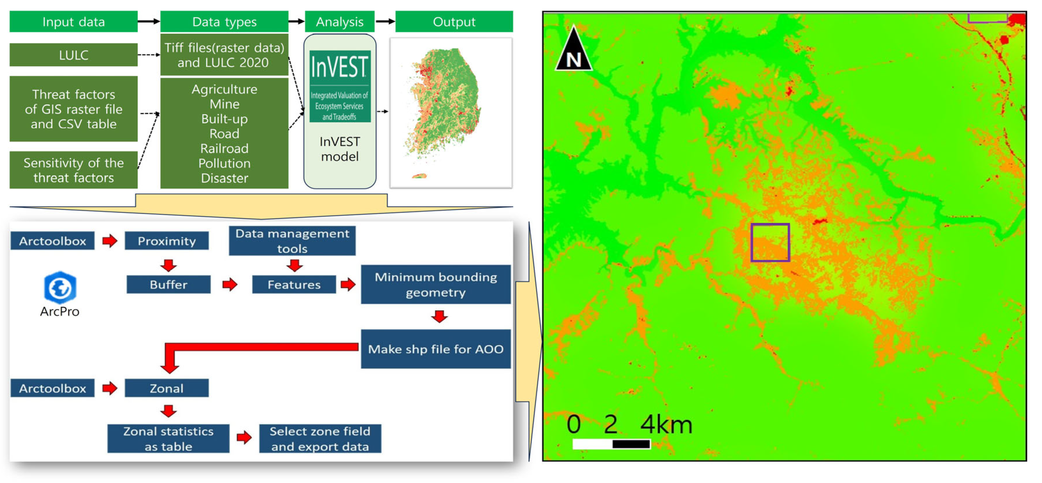
Table 3. Biophysical table of threat factors.
Maximum
Distance (km)
WeightThreat FactorLinear/ExponentialDescription
30.65AgriculturelinearAgricultural lands
60.48MinelinearMine line
80.90Built-upexponentialUrban/developed
30.75RoadlinearRoad line
20.52RailroadlinearRailroad line
50.63PollutionexponentialPollution lands
20.40DisasterlinearDisaster line
Table 4. Importance values for the three vegetation communities classified at the study sites.
SpeciesCom. 1Com. 2Com. 3
Zabelia tyaihyonii (Nakai) Hisauti & H.Hara9.9112.8224.86
Quercus dentata Thunb.12.64-10.20
Thuja orientalis L.5.942.80-
Fraxinus rhynchophylla Hance3.838.343.42
Buxus koreana Nakai ex Chung & al.3.936.90-
Carex humilis var. nana (H.Lév. & Vaniot) Ohwi4.19-6.48
Juniperus rigida Siebold & Zucc.3.992.433.15
Spiraea chinensis Maxim.2.47.1.94
Quercus variabilis Blume2.35--
Securinega suffruticosa (Pall.) Rehder2.25--
Carex lanceolata Boott-3.83-
Thalictrum petaloideum L.-3.03-
Euonymus alatus f. ciliatodentatus (Franch. & Sav.) Hiyama-2.61-
Spodipogon sibiricus Trin.-2.55-
Neillia uyekii Nakai-2.07-
Ulmus macrocarpa Hance--2.42
Pinus densiflora Siebold & Zucc.--2.30
Rhamnus yoshinoi Makino--1.99
Rubia cordifolia var. pratensis Maxim.--1.76
Omitted Species (No.)48.51 (108)52.61 (109)41.48 (75)
Total100100100
Table 5. Indicator species analysis for each community.
ContentsSpecies IVp
Com. 1Quercus dentata Thunb. 53.90.0040
Spiraea chinensis Maxim. 47.60.0206
Quercus variabilis Blume 46.20.0220
Miscanthus sinensis Andersson 46.20.0022
Platycarya strobilacea Siebold & Zucc. 38.50.0068
Thuja orientalis L. 37.60.0490
Leibnitzia anandria (L.) Turcz. 31.80.0480
Com. 2Buxus koreana Nakai ex Chung & al. 48.00.0048
Zabelia tyaihyonii (Nakai) Hisauti & H.Hara40.30.0002
Carex lanceolata Boott 40.00.0096
Neillia uyekii Nakai 40.00.0090
Com. 3Crepidiastrum sonchifolium (Bunge) Pak & Kawano 62.50.0004
Carex humilis var. nana(H.Lév. & Vaniot) Ohwi 51.90.0082
Euonymus alatus (Thunb.) Siebold 47.60.0276
Atractylodes ovata (Thunb.) DC. 40.50.0146
Rhus javanica L. 40.20.0176
Ulmus macrocarpa Hance 39.90.0184
Pinus densiflora Siebold & Zucc. 39.50.0260
IV, indicator value.
Table 6. Environmental factors across Z. tyaihyonii habitats by community.
ContentsCom. 1Com. 2Com. 3Fp-Value
Geography
and
vegetational
Factors
Altitude (m) ns217.2 ± 7.7221.2 ± 9.5257.5 ± 25.82.3020.116
Slope (°) ns8.0 ± 1.15.8 ± 0.86.0 ± 1.41.5170.234
TWI ns7.93 ± 0.439.16 ± 0.618.93 ± 1.111.0480.362
TPI ns−1.59 ± 2.45−3.22 ± 0.94−0.61 ± 2.200.4720.628
Northness ns−0.72 ± 0.10−0.63 ± 0.12−0.39 ± 0.201.4430.251
Canopy openness (%) ns45.88 ± 5.6447.41 ± 4.7454.25 ± 4.310.5690.572
Transmitted light
(mole·m−2·d−1) ns
14.87 ± 1.8815.12 ± 1.6618.29 ± 1.750.8620.432
Soil propertiesOrganic matter (%) ns18.5 ± 1.016.9 ± 1.518.4 ± 0.60.5390.588
Gravel fraction (%) ns47.4 ± 3.543.6 ± 3.150.9 ± 4.80.9130.411
pH ns7.77 ± 0.057.82 ± 0.097.68 ± 0.041.3770.266
EC (ds/m) ns0.64 ± 0.070.76 ± 0.080.67 ± 0.080.6690.519
K+ (cmol+/kg) ns0.327 ± 0.0250.406 ± 0.0550.343 ± 0.0370.9730.388
Ca2+ (cmol+/kg) *16.462 ± 1.398 a20.208 ± 1.564 b15.390 ± 1.396 a3.3300.048
Mg2+ (cmol+/kg) ns5.208 ± 0.5294.455 ± 0.4686.238 ± 0.4892.6790.084
Na+ (cmol+/kg) ns0.038 ± 0.0050.051 ± 0.0060.044 ± 0.0081.3820.265
Al3+ (cmol+/kg) ns7.476 ± 1.8136.898 ± 1.7156.324 ± 1.7320.0860.916
CEC (cmol+/kg) ns0.038 ± 0.0050.051 ± 0.0060.044 ± 0.0080.6550.526
Species diversitySpecies richness *31.77 ± 2.42 b23.00 ± 2.25 a28.00 ± 1.24 a4.3280.021
Shannon index *2.99 ± 0.11 b2.57 ± 0.08 a2.66 ± 0.10 a4.3160.022
Evenness **0.87 ± 0.01 b0.77 ± 0.02 a0.86 ± 0.01 b11.703<0.001
ns, non-significant; TWI, topographic wetness index; TPI, topographic position index; EC, electrical conductivity; CEC, cation exchange capacity. Different letters(a and b) above the bars indicate significant differences. *: p < 0.05; **: p < 0.01.
Disclaimer/Publisher’s Note: The statements, opinions and data contained in all publications are solely those of the individual author(s) and contributor(s) and not of MDPI and/or the editor(s). MDPI and/or the editor(s) disclaim responsibility for any injury to people or property resulting from any ideas, methods, instructions or products referred to in the content.

