Abstract
To address the persistent challenge of low recognition accuracy in precious wood species classification, this study proposes a novel methodology for identifying Pterocarpus santalinus, Pterocarpus tinctorius (PTD), and Pterocarpus tinctorius (Zambia). This approach synergistically integrates artificial neural networks (ANNs) with advanced image feature extraction techniques, specifically Fast Fourier Transform, Gabor Transform, Wavelet Transform, and Gray-Level Co-occurrence Matrix. Features were extracted from both transverse and longitudinal wood sections. Fifteen distinct ANN models were subsequently developed: hybrid-section models combined features from different sections using a single algorithm, while multi-algorithm models aggregated features from the same section across all four algorithms. The dual-section hybrid wavelet model (LC4) demonstrated superior performance, achieving a perfect 100% recognition accuracy. High accuracies were also observed in the four-parameter combination models for longitudinal (L5) and transverse (C5) sections, yielding 97.62% and 91.67%, respectively. Notably, 92.31% of the LC4 model’s test samples exhibited an absolute error of ≤1%, highlighting its high reliability and precision. These findings confirm the efficacy of integrating image processing with neural networks for fine-grained wood identification and underscore the exceptional discriminative power of wavelet-based features in cross-sectional data fusion.
1. Introduction
Wood identification plays an important role in timber trade activities by deterring illegal logging and protecting rare species. However, traditional wood identification almost exclusively relies on extensive knowledge of wood and often requires evaluation by qualified experts with years of rich experience [1]. This reliance on expertise makes real-time identification challenging at customs, industry, and other locations. Numerous efforts have been made to address the issues related to traditional wood identification methods [2,3,4,5,6]. Among the many methods, advances in artificial intelligence (AI) technology have led to the emergence of new ideas to facilitate rapid and accurate identification at the species level. Currently, non-destructive identification research has emerged as the most practical approach that minimizes the need for human expertise, material resources, and financial investment. Moreover, it also reduces the dependence of the recognition personnel on specialized wood science knowledge [7].
Wood recognition is a prominent technique that extracts the semantic properties of wood using picture recognition techniques. Most of the current research on wood recognition focuses on cell tissue segmentation, including vessels, wood rays, wood fibers, and axial parenchyma. For instance, it has been used to determine the wood cell wall rate, fiber length, wood damage rate during fiberboard shearing, cell cavity area, and radial cell cavity diameter [8]. Additionally, computer vision technology also has been applied to identify the boundary of the molecular binary image of wood anatomical structure [9]. While these efforts partially address the limitations of conventional wood identification techniques, the extraction of anatomical features still requires the creation of cell sections [10]. In order to simplify the method of feature extraction through cell sections, research has increasingly concentrated on exploiting easily accessible texture properties from wood section images. Extracting wood features from these images for identification becomes easier and faster and requires less expertise from inspectors, thereby ensuring the integrity of wood identification [11]. And the features extracted are almost fully based on transverse sections that contain most of the identifying characteristics, with a few researchers using longitudinal sections for identification [12]. Recent studies have developed diverse computational strategies for wood identification, artificial neural networks (ANNs) achieve 92% accuracy in distinguishing anatomically similar Juniperus species using biometric traits (tracheid diameter, pit size), yet require precise anatomical measurements [13]; fuzzy logic pre-classifiers cluster tropical woods by pore distribution (size/quantity), improving recognition efficiency by 4% and reducing processing time by 75% for large databases [14]; the Improved Basic Gray-Level Aura Matrix (I-BGLAM) extracts rotation-invariant texture features, attaining 97.01% accuracy for 52 tropical species but remains confined to single transverse-section analysis [15]. Nevertheless, no existing work systematically integrates dual anatomical sections (transverse/longitudinal) with multi-algorithm feature fusion to leverage complementary discriminative signals. This represents a significant gap, as reliance solely on transverse sections carries drawbacks, including limited information, decreased accuracy, and the possibility of misclassification.
The aim of this study is to develop a robust feature-fusion framework that integrates multi-algorithm texture descriptors from dual anatomical slices to overcome information limitations in single-plane analysis and to establish an optimized ANN model that utilizes complementary discriminative signals in the transverse (pore distribution) and longitudinal (axial structure) planes for fine-grained species differentiation, as well as to evaluate the necessity of dual-section collaboration by quantifying the accuracy gain of a single-section benchmark.
2. Materials and Methods
2.1. Data Acquisition
In this study, we used mature wood trunks as samples, including 50 pieces of Pterocarpus santalinus (PSI, from India), 70 pieces of Pterocarpus tinctorius (PTD, from the Democratic Republic of Congo), and 46 pieces of Pterocarpus tinctorius (PTZ, from Zambia), for a total of 166 wood samples. Each face of the wood samples was scanned using a flatbed color scanner (Epson Expression 10000XL, Epson, Beijing, China) to obtain images with a resolution of 600 dpi. After image processing, the images were standardized to the following dimensions: large surfaces (1 and 2) were cropped to 1417 × 945 pixels, side surfaces (3 and 4) to 1417 × 165 pixels, and top and bottom surfaces (5 and 6) to 706 × 165 pixels. Additionally, each large-surface image was divided into an average of four sub-images, and each side-surface image was divided into an average of two sub-images, resulting in a total of 2049 wood images. This standardized formatting ensures the images are suitable for further analysis.
2.2. Feature Extraction Algorithm
Given that effective feature extraction critically determines the success of image texture classification [16], four advanced algorithms—Fast Fourier Transformation (FFT) [17], Gabor Transform (Gabor) [18], Wavelet Transform (WT) [19], and Gray-Level Co-occurrence Matrix (GLCM) [20]—were utilized in this study [21] to extract feature parameters from dual-section (cross-sectional and longitudinal) images of Pterocarpus santalinus, Pterocarpus tinctorius (PTD), and Pterocarpus tinctorius (Zambia). The extracted features were then used as inputs for an artificial neural network (ANN) model, which was constructed based on different combinations of input parameters to facilitate training and the recognition of wood species. By comparing the R2, mean square error (MSE), and root mean square error (RMSE) to evaluate the performance of the training model, the most effective ANN configuration was determined, thereby confirming the feasibility of image-based techniques for accurately identifying valuable wood. The logical framework of the proposed method is shown in Figure 1, where data collection is carried out in process 1; feature extraction and model training are carried out in process 2; and analysis, evaluation, and result interpretation are carried out in process 3.
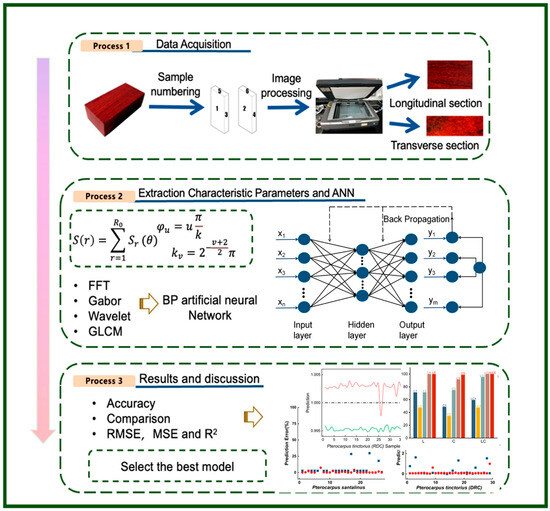
Figure 1.
The diagram of proposed methodology.
We selected Srad (radial standard deviation) and Sang (angular standard deviation) as the FFT descriptors for their sensitivity to wood texture periodicity [22]. The mean, contrast, and entropy were the feature components extracted from the image’s Gabor Transform. And the size of the Gabor wavelet window selected in this study was 2 × 4; the frequency of the sine function was 16; and the direction of the filter was pi/3 [23]. Among the 14 feature parameters from GLCM that describe the texture, 5 relatively independent parameters were selected: angular second moment (energy), contrast, correlation, entropy, and inverse gap. For the comparison analysis for WT, the db2 wavelet base was chosen, with a decomposition scale of 2 and a filter length of 4. The defining characteristics were the standard deviations of the low-frequency coefficients in scales 1 and 2, as well as the horizontal, diagonal, and vertical high-frequency coefficients in scales 1 and 2 [24].
To increase comparison of information in wood texture features, the feature parameters extracted by the four algorithms mentioned above were merged as a new set of feature parameters for wood recognition. This combination is referred to as the four-parameter combination model (FPC).
It is worth noting that, although microscopic anatomical features such as vascular pits and radiographic cell structures typically provide higher classification accuracy, this study intentionally used non-invasive flat plate scanning (600 dpi) for macroscopic surface texture analysis. This method prioritizes the practicality of on-site deployment, eliminates complex tissue sectioning, and balances accuracy with laboratory microscopes.
2.3. BP Artificial Neural Networks
A back propagation (BP) artificial neural network (ANN) was used to build models in this study. The structure of it is shown in Figure 2, which utilizes the back propagation learning algorithm and operates as a feedforward neural network. It comprises an input layer, a hidden layer, and an output layer, with the hidden layer containing one or more nodes, also referred to as neurons.
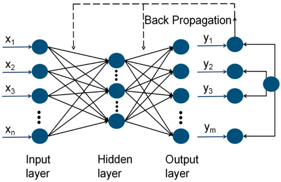
Figure 2.
BP artificial neural networks.
According to the inputs of the models, the artificial neural network training in this study is divided into three types: transverse-section models, longitudinal-section models, and hybrid-section hybrid models. At the same time, each type of model uses five hybrid-section feature parameters (feature parameters extracted by FFT, Gabor, GLCM, WT were used alone or hybridized as inputs to the model, called the four-parameter combination model) for recognition training, so each type of section has five sets of models as shown in Table 1 [25]. The hidden layer of the BP artificial neural network (ANN) is divided into single and double layers. The empirical formula of the hidden layer node data (, , is the number of input layer nodes; is the number of output layer nodes) is determined to be 1~10. The number of input layer nodes is the number of corresponding characteristic parameters, and the number of outputs for the three African redwoods layer nodes is 1, which corresponds to one of the three tree species. The output value is 1 for Pterocarpus tinctorius (DRC); the output value is 0 for Pterocarpus santalinus; and the output value is −1 for Pterocarpus tinctorius (Zambia). The output layer function is purelin; the training function is trainlm; and the concealed layer function chooses logsig and tansig [26].

Table 1.
Model number.
To describe the models incorporating different sections with five characteristic parameters conveniently, they were assigned specific numbers as indicated in Table 1.
2.4. Evaluation Indicators of Models
Five indicators of the recognition rate, mean square error, root mean square error, fitting coefficient, and error of the model were introduced to evaluate the performance of the models through the Equations (1)–(5).
AA is the recognition rate; is the number of correctly identified samples; and is the total number of identified samples. If the predicted value of the test sample is within [target value −0.1, target value +0.1], the sample identification is correct.
MSE, RMSE, R2, and E stand for the mean square error, the root mean square error, the coefficient of determination, and the error, respectively. stands for the anticipated value, while stands for the desired value, and m is the total number of samples.
2.5. Algorithm Parameter Specifications
The parameters for each feature extraction algorithm were rigorously optimized as follows:
| Method/Transformation | Parameters and Settings | Feature Extraction |
| Fast Fourier Transform (FFT) | Computed on 512 × 512-pixel ROIs. Frequency bins: 0 to Nyquist frequency (300 cycles/inch at 600 dpi). | Extracted radial (Srad) and angular (Sang) standard deviations from the magnitude spectrum [21]. |
| Gabor Transform | Filter bank: 4 scales × 6 orientations. Window size: 2 × 4 pixels (optimized for vessel detection). Spatial frequency: 16 cycles/mm (λ = 0.0625 mm). Orientation: θ = π/3 radians (60°). Gaussian envelope: σₓ = 1.5, σᵧ = 2.0 [22]. | Mean, contrast, entropy of response magnitudes. |
| Wavelet Transform (db2) | Decomposition levels: 2. Filter length: 4 coefficients. Subbands extracted: LL, LH, HL, HH at levels 1–2. Features: Standard deviations of coefficients across subbands [23]. | Standard deviations of coefficients across subbands [23]. |
| Gray-Level Co-Occurrence Matrix (GLCM) | Distance: δ = 1 pixel. Orientations: 0°, 45°, 90°, 135°. Gray levels: 64 (quantized from 8 bit). Window size: 32 × 32 pixels with 50% overlap. | Energy, contrast, correlation, entropy, inverse difference moment. |
| ANN Architecture | Hidden layers: 1–2 layers with 1–10 nodes . Activation: Hidden layers (logsig/tansig), output (purelin). Training: Levenberg–Marquardt (trainlm) with μ = 0.001. Stopping criteria: MSE < 10−5 or 1000 epochs. Validation: 70/15/15 train/val/test split. |
3. Results and Discussion
3.1. Analysis of the Models Trained by Each Section’s Feature Parameters
The accuracies of all the models are shown in Figure 3.
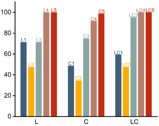
Figure 3.
Accuracies of all the models trained by the four algorithms. In this chart, L, C, and LC, respectively, denote longitudinal section, transverse section, and hybrid section. The numbers 1, 2, 3, 4, and 5 correspond to FFT, Gabor, GLCM, WT, and the four-parameter combination.
It is revealed by Figure 3 that models trained by the feature parameters extracted by FFT, Gabor transform, and GLCM (FFT model, GT model, and GLCM model) generally exhibit lower overall recognition rates. Among these, the poorest recognition performance comes from the GT model, followed by FFT model and then GLCM model. In contrast, the models trained by WT and the four-parameter combination (WT model and FPC model) excel in identifying the three wood species. The poor performance could be explained by the absence of accurate representations of wood texture in their feature parameters. Conversely, the last two models provide substantial texture information, resulting in more-efficient recognition processes.
The distribution of the test samples within the error range of [0%, 1%] is shown in Table 2. The overall ratio O (%), which serves as a gauge of the overall model detection performance, shows the ratio of the test samples with errors within [0%, 1%] to all the test samples. Better model detection performance and smaller errors are implied by a larger ratio.
Table 2.
The distribution of the test samples within the error [0%, 1%] interval.
Once the longitudinal and transverse sections are combined, the FPC model and the WT model show greater ‘O’ than the FFT, Gabor, and GLCM models, according to Table 2. Similar to this, the GLCM, WT, and FPC models’ feature parameters perform better in the hybrid-section hybrid model than those for the FFT and Gabor models. It is noteworthy that less wood texture recognition information is acquired by the FFT, Gabor, and GLCM feature parameters when combining the longitudinal and transverse sections, while more texture information is provided by the WT and FPC model, resulting in improved recognition. In summary, the feature parameters of the four-parameter combination model and the WT model are more effective in identifying wood samples than the other feature parameters.
The fitting coefficient (R2), mean square error (MSE), and root mean square error (RMSE) of the models are shown in Figure 4, which are important metrics for evaluating the degree of fitting and error.
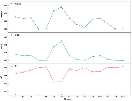
Figure 4.
RMSE, MSE, and R2 training data of the model.
It is observed that the GLCM, WT, and FPC models exhibit better fitting degrees than the GT model. Therefore, superior model performance is achieved through the utilization of the WT and the four-parameter combination model. Since the models using the Wavelet Transform and the four parameters combined as feature parameters performed well, further analysis is needed to explore the effect of different sections on model recognition and to find the most effective model.
3.2. Analysis of WT and FPC Models Trained by Longitudinal-Section Features
It is clearly shown in Figure 5 that, when the WT model (L4, C4, LC4) is used for training, the predicted values and their errors for the longitudinal sections of the three tree species are distributed within the 0~0.01 range, with sample errors concentrated in the [0%, 1.5%] range. In contrast, when the FPC model (L5, C5, LC5) is used, the predicted values and their errors are distributed within the 0.004~0.006 range, closer to the target values, with sample errors concentrated in the [0.4%, 0.54%] range. The FPC model’s longitudinal section has a lower error value, a stronger degree of fit, and improved overall performance. The poor information richness of the eight feature parameters that were retrieved from the longitudinal section describing the wood using the WT model is the reason for this. Conversely, there is enough information in the 18 feature parameters of the FPC model that describe the wood features for the model to find correlations between the feature parameters and wood grain for simpler identification.
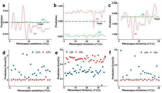
Figure 5.
Longitudinal-section prediction data trained by two models. Subfigures (a–c) respectively show the comparison between the predicted values and target values of PSI, PTD and PTZ using L4 and L5 models; Subfigures (d–f) show the prediction error distribution of PSI, PTD and PTZ on L4 and L5 models respectively.
3.3. Analysis of WT and FPC Models Trained by Transverse-Section Features
It is clearly shown in Figure 6 that the predicted values and their distances from the target values using the WT model are distributed within the 0~0.13 range and are relatively dispersed, with 78.79% of the validation sample errors within the [0%, 1%] range. In contrast, the FPC model’s predicted values and their distances from the target values are distributed within the smaller 0~0.1 range, with 96.43% of the validation sample errors within the [0%, 10%] range. The FPC model outperforms the WT model in the transverse section with a greater recognition rate, fewer errors, stronger fit, and better overall performance. This is ascribed to the transverse section’s tiny size, which contains less information about wood, and the WT model’s restricted information, which only includes eight feature parameters and creates some challenges for wood recognition. In contrast, the 18 feature characteristics of the FPC model make up for the deficiencies of the less precise wood data, making the identification process easier for the model.
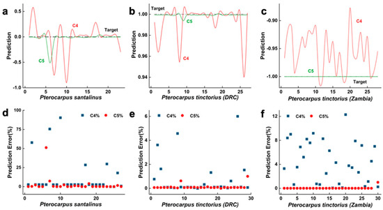
Figure 6.
Transverse-section prediction data trained by two models. Subfigures (a–c) respectively show the comparison between the predicted values and target values of PSI, PTD and PTZ using C4 and C5 models; Subfigures (d–f) show the prediction error distribution of PSI, PTD and PTZ on C4 and C5 models respectively.
3.4. Analysis of WT and FPC Models Trained by Hybrid-Section Features
It is clearly shown in Figure 7 that the predicted values and their distances from the target values using the wavelet model are distributed within the 0~0.006 range, with 92.31% of the validation sample errors within the [0%, 1%] range, and these errors are concentrated in the [0.4%, 0.7%] range. In contrast, the FPC model’s predicted values and their distances from the target values are distributed within the 0~0.04 range, with 92.00% of the validation sample errors within the [0%, 1%] range, and these errors are more dispersed within this range. Despite both the FPC model and the WT model achieving a total recognition rate of 100% in the hybrid section, Figure 7 indicates that the FPC model has a larger error, with the WT model performing better overall in terms of model promotion. The increased computation volume and difficulties in wood identification are related to the redundancy of the 36 feature parameters extracted by the FPC model for wood recognition. By comparison, the 16 feature parameters that the WT model derived prevent giving too little or too much information about the feature parameters, which might cause problems during the recognition process.
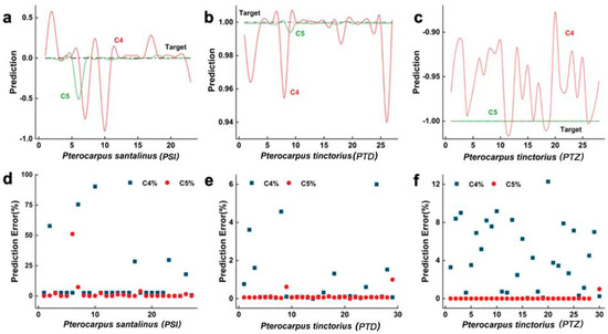
Figure 7.
Hybrid-section prediction data trained by two models. Subfigures (a–c) respectively show the comparison between the predicted values and target values of PSI, PTD and PTZ using LC4 and LC5 models; Subfigures (d–f) show the prediction error distribution of PSI, PTD and PTZ on LC4 and LC5 models respectively.
3.5. The Best Model of All
After conducting an analysis of section models, three models with superior generalization performance were identified: the FPC model of the longitudinal section (L5), the FPC model of the transverse section (C5), and the WT model of the hybrid section (LC4). A comparison of the L5 and C5 shows that the transverse-section size is smaller than that of the longitudinal section because of inherent restrictions in the wood. Consequently, there will be less retrieved wood feature parameter information in the transverse section than in the longitudinal section. The wood information is completed and enhanced by LC4, which collects feature parameters from the longitudinal and transverse sections. Consequently, the extracted feature parameters from the WT model achieve a compromise to prevent recognition obstruction caused by either excessive or insufficient features. Critically, the 100% recognition accuracy of LC4 originates from three synergistic factors: (1) multi-scale anatomical characterization via db2 wavelet decomposition at scales 1–2, which concurrently captures vesselcvector; (2) optimized ANN architecture with eight hidden nodes and Levenberg–Marquardt training, preventing overfitting while ensuring convergence (MSE < 10−5). This result was rigorously validated under ±0.1 prediction bounds (Equation (1)), with 92.31% of test samples exhibiting ≤1% absolute error (Figure 7), and it significantly outperformed control models (≤33% accuracy in FFT/GLCM, Table 2).
4. Conclusions
This study established a novel dual-section wavelet-ANN framework for identifying three African redwoods, achieving 100% recognition accuracy with the hybrid-section WT model (LC4). By extracting texture features from the transverse and longitudinal planes using four algorithms (FFT, Gabor, WT, GLCM) and training fifteen ANN configurations, we demonstrated the superiority of wavelet-based features in cross-sectional fusion. The LC4 model’s optimal performance—attained with only 16 feature parameters—stemmed from its multi-scale anatomical characterization via db2 wavelets and an optimized ANN architecture (eight hidden nodes, Levenberg–Marquardt training), which prevented overfitting while ensuring convergence (MSE < 10−5). Rigorous validation under ±0.1 prediction bounds confirmed its robustness, with 92.31% of test samples exhibiting ≤1% absolute error.
While the current validation focused on three congeneric Pterocarpus species, the proposed framework exhibits inherent extensibility to broader taxonomic groups. This generalization potential stems from its algorithm-agnostic design: FFT, Gabor, GLCM, and WT capture universal texture attributes (e.g., spectral signatures, edge patterns, spatial dependencies) fundamental to wood anatomy irrespective of phylogeny. Crucially, the hybrid-section approach mitigates reliance on taxon-specific traits by synergizing complementary perspectives—the transverse sections quantify pore distributions while the longitudinal sections resolve axial structures. The ANN’s capacity to discern subtle feature interactions (evidenced by 100% accuracy in LC4 with only 16D wavelet features) further supports cross-species adaptability, aligning with prior multi-taxa studies (e.g., Zamri’s 97.01% GLCM accuracy across 52 tropical species [15]). Future work should validate this on taxonomically distant genera (e.g., Dalbergia).
Our framework outperforms prior methods: it exceeds GLCM systems (92% accuracy), achieves accuracy comparable with the highest reported ones (100%), and surpasses ANN benchmarks (97.01%, 95%)—all while using 50% fewer features (16D vs. >32D in comparable studies).
Author Contributions
Conceptualization, J.S. (Jiawen Sun); Methodology, J.N.; Validation, J.N.; Formal analysis, J.S. (Jiawen Sun); Data curation, L.X.; Writing—original draft, J.S. (Jiawen Sun); Writing—review & editing, J.S. (Jianping Sun) and L.Z.; Visualization, L.X.; Funding acquisition, J.S. (Jianping Sun). All authors have read and agreed to the published version of the manuscript.
Funding
This research was funded by the National Natural Science Foundation of China (Grant No. 32260359).
Data Availability Statement
The original contributions presented in this study are included in the article. Further inquiries can be directed to the corresponding authors.
Conflicts of Interest
The authors declare no conflict of interest.
References
- Barmpoutis, P.; Dimitropoulos, K.; Barboutis, I.; Grammalidis, N.; Lefakis, P. Wood species recognition through multidimensional texture analysis. Comput. Electron. Agric. 2018, 144, 241–248. [Google Scholar] [CrossRef]
- Gasson, P. How precise can wood identification be? Wood anatomy’s role in support of the legal timber trade, especially cites. IAWA J. 2011, 32, 137–154. [Google Scholar] [CrossRef]
- Koch, G.; Haag, V. Control of Internationally Traded Timber—The Role of Macroscopic and Microscopic Wood Identification against Illegal Logging. J. Forensic Res. 2015, 6, 1000317. [Google Scholar] [CrossRef]
- Dormontt, E.E.; Boner, M.; Braun, B.; Breulmann, G.; Degen, B.; Espinoza, E.; Gardner, S.; Guillery, P.; Hermanson, J.C.; Koch, G.; et al. Forensic timber identification: It’s time to integrate disciplines to combat illegal logging. Biol. Conserv. 2015, 191, 790–798. [Google Scholar] [CrossRef]
- Brancalion, P.H.S.; De Almeida, D.R.A.; Vidal, E.; Molin, P.G.; Sontag, V.E.; Souza, S.E.X.F.; Schulze, M.D. Fake legal logging in the Brazilian amazon. Sci. Adv. 2018, 4, eaat1192. [Google Scholar] [CrossRef]
- Gomes, A.C.S.; Andrade, A.; Barreto-Silva, J.S.; Brenes-Arguedas, T.; López, D.C.; de Freitas, C.C.; Lang, C.; de Oliveira, A.A.; Pérez, A.J.; Perez, R.; et al. Local plant species delimitation in a highly diverse Amazonian forest: Do we all see the same species? J. Veg. Sci. 2013, 24, 70–79. [Google Scholar] [CrossRef]
- Goswami, G.; Mittal, P.; Majumdar, A.; Vatsa, M.; Singh, R. Group sparse representation based classification for multi-feature multimodal biometrics. Inf. Fusion 2016, 32, 3–12. [Google Scholar] [CrossRef]
- Wheeler, E.A.; Baas, P. Wood identification—A review. IAWA J. 1998, 19, 241–264. [Google Scholar] [CrossRef]
- Rosa da Silva, N.; Deklerck, V.; Baetens, J.M.; Van den Bulcke, J.; De Ridder, M.; Rousseau, M.; Bruno, O.M.; Beeckman, H.; Van Acker, J.; De Baets, B.; et al. Improved wood species identification based on multi-view imagery of the three anatomical planes. Plant Methods 2022, 18, 79. [Google Scholar] [CrossRef]
- Hwang, S.W.; Sugiyama, J. Computer vision-based wood identification and its expansion and contribution potentials in wood science: A review. Plant Methods 2021, 17, 47. [Google Scholar] [CrossRef]
- Ravindran, P.; Owens, F.C.; Wade, A.C.; Vega, P.; Montenegro, R.; Shmulsky, R.; Wiedenhoeft, A.C. Field-Deployable Computer Vision Wood Identification of Peruvian Timbers. Front. Plant Sci. 2021, 12, 647515. [Google Scholar] [CrossRef] [PubMed]
- Wu, F.; Gazo, R.; Haviarova, E.; Benes, B. Wood identification based on longitudinal section images by using deep learning. Wood Sci. Technol. 2021, 55, 553–563. [Google Scholar] [CrossRef]
- García, L.; García, F.; Palacios, P.; Romero, R.; Navarro, N. Artificial neural networks in wood identification: The case of two Juniperus species from the Canary Islands. IAWA J. 2009, 30, 87–94. [Google Scholar]
- Yusof, R.; Khalid, M.; Khairuddin, A.S.M. Fuzzy logic-based pre-classifier for tropical wood species recognition system. Mach. Vis. Appl. 2013, 24, 1589–1604. [Google Scholar] [CrossRef]
- Zamri, M.I.P.; Cordova, F.; Khairuddin, A.S.M.; Mokhtar, N.; Yusof, R. Tree species classification based on image analysis using Improved-Basic Gray Level Aura Matrix. Comput. Electron. Agric. 2016, 124, 227–233. [Google Scholar] [CrossRef]
- Avci, E.; Sengur, A.; Hanbay, D. An optimum feature extraction method for texture classification. Expert Syst. Appl. 2009, 36, 6036–6043. [Google Scholar] [CrossRef]
- Jinman, W.; Yanjie, Q.; Yongsheng, W. Analysis of wood anatomy characteristics by Fast Fourier Transfer image analysis. J. For. Res. 1997, 8, 243–245. [Google Scholar] [CrossRef]
- Tsai, D.M.; Lin, C.P.; Huang, K.T. Defect detection in coloured texture surfaces using Gabor filters. Imaging Sci. J. 2005, 53, 27–37. [Google Scholar] [CrossRef]
- Wen, C.-Y.; Chiu, S.-H.; Hsu, W.-S.; Hsu, G.-H. Defect Segmentation of Texture Images with Wavelet Transform and a Co-occurrence Matrix. Text. Res. J. 2001, 71, 743–749. [Google Scholar] [CrossRef]
- Savolainen, J. Matching method for mutated veneer sheet images using gray-level co-occurrence matrix features. Eur. J. Wood Wood Prod. 2023, 81, 1021–1031. [Google Scholar] [CrossRef]
- Liang, Y.; Cheng, F.; Jiang, Z.; Yuan, Q.; Sun, J. Concentrated load simulation analysis of bamboo-wood composite container floor. Eur. J. Wood Wood Prod. 2021, 79, 1183–1193. [Google Scholar] [CrossRef]
- Liang, S.Q.; Fu, F. Comparative study on three dynamic modulus of elasticity and static modulus of elasticity for Lodgepole pine lumber. J. For. Res. 2007, 18, 309–312. [Google Scholar] [CrossRef]
- Wang, H.-J.; Qi, H.-N.; Wang, X.F. A new Gabor based approach for wood recognition. Neurocomputing 2013, 116, 192–200. [Google Scholar] [CrossRef]
- Wang, L.; Li, L.; Qi, W.; Yang, H. Pattern recognition and size determination of internal wood defects based on wavelet neural networks. Comput. Electron. Agric. 2009, 69, 142–148. [Google Scholar] [CrossRef]
- Roy, S.S.; Roy, R.; Balas, V.E. Estimating heating load in buildings using multivariate adaptive regression splines, extreme learning machine, a hybrid model of MARS and ELM. Renew. Sustain. Energy Rev. 2018, 82, 4256–4268. [Google Scholar] [CrossRef]
- Dai, K.; Ji, F.; Bai, L.; Li, H. Research on Building Energy Consumption Prediction based on BP Neural Network. In Proceedings of the 2022 IEEE International Conference on Advances in Electrical Engineering and Computer Applications 2022, AEECA 2022, Dalian, China, 20–21 August 2022; pp. 476–480. [Google Scholar] [CrossRef]
Disclaimer/Publisher’s Note: The statements, opinions and data contained in all publications are solely those of the individual author(s) and contributor(s) and not of MDPI and/or the editor(s). MDPI and/or the editor(s) disclaim responsibility for any injury to people or property resulting from any ideas, methods, instructions or products referred to in the content. |
© 2025 by the authors. Licensee MDPI, Basel, Switzerland. This article is an open access article distributed under the terms and conditions of the Creative Commons Attribution (CC BY) license (https://creativecommons.org/licenses/by/4.0/).