Article

Unveiling Scale-Dependent Elevational Patterns and Drivers of Tree β Diversity on a Subtropical Mountain Using Sentinel-2 Remote Sensing Data

1
Zhoushan Archipelago Observation and Research Station, Tiantong Forest Ecosystem National Observation and Research Station, School of Ecological and Environmental Sciences, East China Normal University, Shanghai 200241, China
2
Institute of Eco-Chongming (IEC), Shanghai 202162, China
3
Lushan Botanical Garden, Jiangxi Province and Chinese Academy of Sciences, Jiujiang 332900, China
4
School of Life Sciences, Sun Yat-sen University, Guangzhou 510275, China
*
Author to whom correspondence should be addressed.
Forests 2025, 16(6), 917; https://doi.org/10.3390/f16060917
Submission received: 21 April 2025 / Revised: 27 May 2025 / Accepted: 29 May 2025 / Published: 30 May 2025
(This article belongs to the Section Forest Biodiversity)

Abstract

The elevational patterns of plant β diversity and their underlying drivers are known to be scale-dependent, but pinpointing the spatial scales at which different ecological processes occur remains challenging using traditional field inventory methods. Remote sensing has emerged as a promising alternative, providing continuous spatial data for monitoring plant diversity. In this study, we used field inventory data and corresponding Sentinel-2 images from a subtropical mountain to simulate pooled assemblages and assess the potential of using multispectral satellite images in predicting tree β diversity. We further examined the scale-dependent elevational gradient of the spectral β diversity and identified primary topographic variables across different spatial extents (0.16–64 ha). The spectral β diversity showed a consistently positive relationship with the inventory β diversity calculated using various indices (average pairwise Sørensen, Jaccard, and Bray–Curtis dissimilarities, as well as multi-community differentiation measures based on Hill numbers), with the strongest correlation observed for abundance-weighted indices and images from early spring and late autumn (R2max = 0.63). However, a null model-derived β deviation showed only a weak correlation between remote sensing and field-based measures. A declining trend in the spectral β diversity with an increasing elevation was observed and became more pronounced at larger extents. The topographic heterogeneity, represented by the slope and northness, explained the elevational gradients at spatial extents >4 ha, attesting the significant role of environmental filtering in shaping plant diversity patterns, even at fine scales. While the northness was more influential at smaller spatial extents (<4 ha), the slope had a stronger impact at broader spatial extents (>4 ha). This study showcases the potential of using readily available remote sensing data to address difficult questions in plant diversity research.

1. Introduction

Changes in the β diversity, which reflects the variation in the species composition among different localities within a region, are a striking signature of biodiversity [1]. Understanding how the β diversity varies along ecological gradients and through time is crucial for unraveling the spatiotemporal patterns of biodiversity [2,3,4]. Despite intensive investigations over the past few decades [5,6,7,8,9,10], the patterns and mechanisms driving tree β diversity along key ecological gradients, such as the latitude and altitude, remain elusive. These gradients encompass a range of environmental factors that significantly influence the species distribution and community composition, yet the intricate processes driving these patterns are not fully understood.
Previous studies have demonstrated that the latitudinal and elevational gradients of tree β diversity are spatial scale-dependent [7,9,11,12,13]. When calculated for small spatial extents (e.g., <500 m), the tree β diversity may show significant or insignificant trends along ecological gradients, sparking debate about the roles of community assembly processes like environmental filtering and dispersal limitation in shaping these patterns [6,14,15,16,17,18]. However, several studies have provided unambiguous evidence that the tree β diversity at broader spatial extents (e.g., >7 km) varies significantly, albeit non-monotonically, with both the latitude [7,12] and altitude [11]. These non-monotonic patterns can largely be explained by environmental heterogeneity, represented by spatial variation in the climate and soil [7,12,13]. Despite this progress, it remains unclear at what spatial scales the β diversity shows systematic trends and how environmental factors act across different scales to shape β diversity patterns.
Addressing this challenge using traditional field inventory methods is difficult due to the challenges of acquiring spatially continuous data. Typically, field inventories are only conducted in spatially dispersed localities, and broader spatial extents are examined by grouping nearby samples. For example, Tello et al. [11] studied regional communities by grouping 10 local plots near each other at similar elevations to study the scale dependence of the elevational gradient of tree β diversity. These regional communities covered regions extending over 19 km. Along the latitudinal gradient, Xing and He [7] employed a similar approach, grouping forest inventory plots from extensively sampled North American forests to examine regional communities with minimum spatial extents greater than 7 km. However, it remains difficult to infer from this approach how β diversity patterns and their responses to the environment change with spatial extents spanning from a few hundred meters to several kilometers, spatial scales that are crucial for considering in forest conservation and management in fragmented landscapes [19].
Recently, emergent spectral diversity measures derived from optical remote sensing have provided a promising alternative for studying scale dependence along latitudinal and elevational β diversity gradients [20]. Remote sensing addresses many of the limitations of traditional field-based methods, including their labor and resource demands, heterogeneity in terms of data quality, and challenges in their large-scale deployment [21,22]. Several studies have tested the association between spectral diversity and various measures of taxonomic diversity calculated from field inventory data [23,24,25,26]. However, few studies have integrated remote sensing with ecological theory to consider ecological processes [27]. Moreover, limited attempts have been made to study tree β diversity using spectral data, with mixed results on whether the spectral β diversity can serve as a proxy for the observed tree β diversity. For instance, earlier studies quantified the spectral β diversity using the variation in specific spectral indices such as the Normalized Difference Vegetation Index (NDVI), finding weak correlations between the spectral and plant β diversity [28,29]. This was likely because the NDVI uses only two spectral bands and saturates with moderate-to-dense canopies [30]. Recent studies, however, have shown that wavelength regions beyond those used to calculate the NDVI (e.g., red edge and shortwave infrared) are important for predicting plant diversity [25,31]. New methods that make full use of all the available wavelength bands [32,33] have primarily been tested with hyperspectral data across contrasting vegetation types, e.g., in [24,34]. It remains to be demonstrated whether these methods can predict the tree β diversity in closed-canopy forests using readily available multispectral satellite data like those from Sentinel-2.
In this study, we integrated multitemporal and multispectral reflectance data from Sentinel-2 with forest inventory data from 58 plots along a subtropical elevational gradient in eastern China to achieve two main objectives. First, we tested the association between the spectral β diversity and various β diversity measures derived from the inventory data, using a method developed by Laliberté et al. [33] to quantify the spectral β diversity. This method was applied to individual images acquired in different seasons, as well as to stacked images taken across seasons and a full year, to assess the potential contribution of phenology [25]. Second, we used the Sentinel-2 data to assess the spatial-scale dependence in the elevational gradient of the spectral β diversity, focusing on the topographic drivers shaping these patterns. To achieve this objective, we tested two specific hypotheses. Based on previous observations of a lack of elevational β diversity gradients at small extents (e.g., 50 m [6,11]) and evidence of such gradients at large extents (e.g., 19 km [11]), we hypothesized that the elevational gradient of the spectral β diversity would be weak at smaller spatial extents, with a threshold beyond which a strong association between the spectral β diversity and elevation would emerge (Hypothesis 1). Furthermore, inspired by similar studies on latitudinal β diversity gradients [7,12], we hypothesized that the stronger elevational gradients at larger spatial extents would primarily result from environmental filtering. Given that topographic variables such as the slope and aspect are closely linked to the microclimate and soil nutrients—factors known to influence the plant community composition [35,36]—we predicted that any observed elevational gradient of the spectral β diversity could be explained by the topographic heterogeneity (Hypothesis 2).

2. Materials and Methods

2.1. Study Area and Field Survey

This study was conducted in the Tianmu National Nature Reserve, located in Zhejiang province, eastern China (30°18′30″–30°21′37″ N, 119°24′11″–119°27′11″ E). The reserve covers approximately 4300 ha and features an elevational gradient from 400 to 1506 m above sea level. The region’s annual mean temperature ranges from 8.8 to 14.5 °C, and the annual precipitation varies between 1390 and 1870 mm [37]. The reserve is covered by 140-year-old natural evergreen and deciduous broad-leaved forests and its predominant composition transitions between evergreen broad-leaved forests, mixed forests of evergreen and deciduous broad-leaved species, and deciduous broad-leaved forests with an increasing elevation [38]. Approximately 90% of the area consists of volcanic rock, and the zonal soils vary with the elevation: red soils dominate below 600 m in elevation, yellow soils occur between 600 and 1200 m in elevation, and brown-yellow soils are found above 1200 m in elevation.
Between 2017 and 2021, we established a total of 58 standard forest plots across the reserve (Figure S1). Each plot was a 20 × 20 m square, with the coordinates of the four corners recorded using a high-precision GeoXH 3000 handheld GPS (Trimble Inc., Sunnyvale, CA, USA). Within each plot, all woody plants with a diameter at breast height (DBH) ≥ 1 cm were tagged, measured, and identified based on their species [39]. To allow for the use of spectral data, which are mostly relevant to forest canopies [25], we only analyzed trees with a DBH ≥ 10 cm. Our dataset included 2783 individuals from 137 species, spanning 80 genera and 42 families. The most species-rich families were Fagaceae, Rosaceae, and Lauraceae, together representing 38 species and accounting for 33% of all individuals. The most abundant species, in descending order, were Quercus myrsinifolia Blume (Fagaceae), Cunninghamia lanceolata (Lamb.) Hook. (Cupressaceae), Carpinus viminea Lindl. ex Wall. (Betulaceae), Daphniphyllum macropodum Miq. (Daphniphyllaceae), Liquidambar formosana Hance (Altingiaceae), Quercus ciliaris C.C.Huang & Y.T.Chang (Fagaceae), and Lithocarpus brevicaudatus (Skan) Hayata (Fagaceae), each with more than 100 individuals.

2.2. Sentinel-2 Spectral Reflectance Data

Sentinel-2 satellites provide high-resolution multispectral imagery with global coverage and a revisit time of five days. They capture spectral information across 13 bands, with their ground sampling resolutions ranging from 10 to 60 m. These include three visible bands (B02—blue; B03—green; B04—red) and one near-infrared band (B08) at a 10 m resolution and three vegetation red edge bands (B05, B06, B07), one narrow near-infrared band (B08A), and two shortwave infrared bands (B11, B12) at a 20 m resolution. Additionally, three coarser bands (B01—coastal aerosols; B09—water vapor; B10—cirrus) at a 60 m resolution record coastal aerosol, water vapor, and cirrus data. We used the ten pre-processed Level-2A (bottom-of-atmosphere reflectance in cartographic geometry [40]) bands at 10 m and 20 m resolutions (Table S1), with the coarser bands resampled to 10 m resolutions using bilinear interpolation.
Given a nominal absolute geolocation accuracy of approximately 12 m at 95% confidence [41], we tested five coordinates (four corners and the centroid) when extracting the spectral data for each plot. Consistent with previous work predicting the tree α diversity in the same region [25], we found that data extracted from the northwest corners provided the best match between the ground and remote sensing data, and these coordinates were used for subsequent analyses.
We downloaded all the Sentinel-2 Level-2A surface reflectance imagery with less than 15% cloud coverage for the study region, acquired between 2019 and 2022, from Google Earth Engine. Each image was further examined for pixels overlapping our field plots using the built-in scene classifier. Images with over 15% non-vegetation pixels in 15 m buffer zones surrounding the plot coordinates were excluded. To address the minimal cloud cover in the remaining images, the cloud pixels were filled with the mean reflectance of the exact same pixels from other, cloud-free images taken in the same month. This process initially resulted in 55 usable images, with 2 additional images included after visual checks for misclassifications, yielding 57 images for analysis. Only 14 of the 57 images had minimal cloud pixels (average of 7%, range of 2%–14%), which were imputed using the method just mentioned. The other images used in our analysis were cloud-free. Hence, the influence of the imputation method on our results was negligible. The relationship between the acquisition season and vegetation phenology, which might explain the link between the spectral and inventory diversity, is summarized in Table 1, while the exact acquisition dates can be found in Table S2.

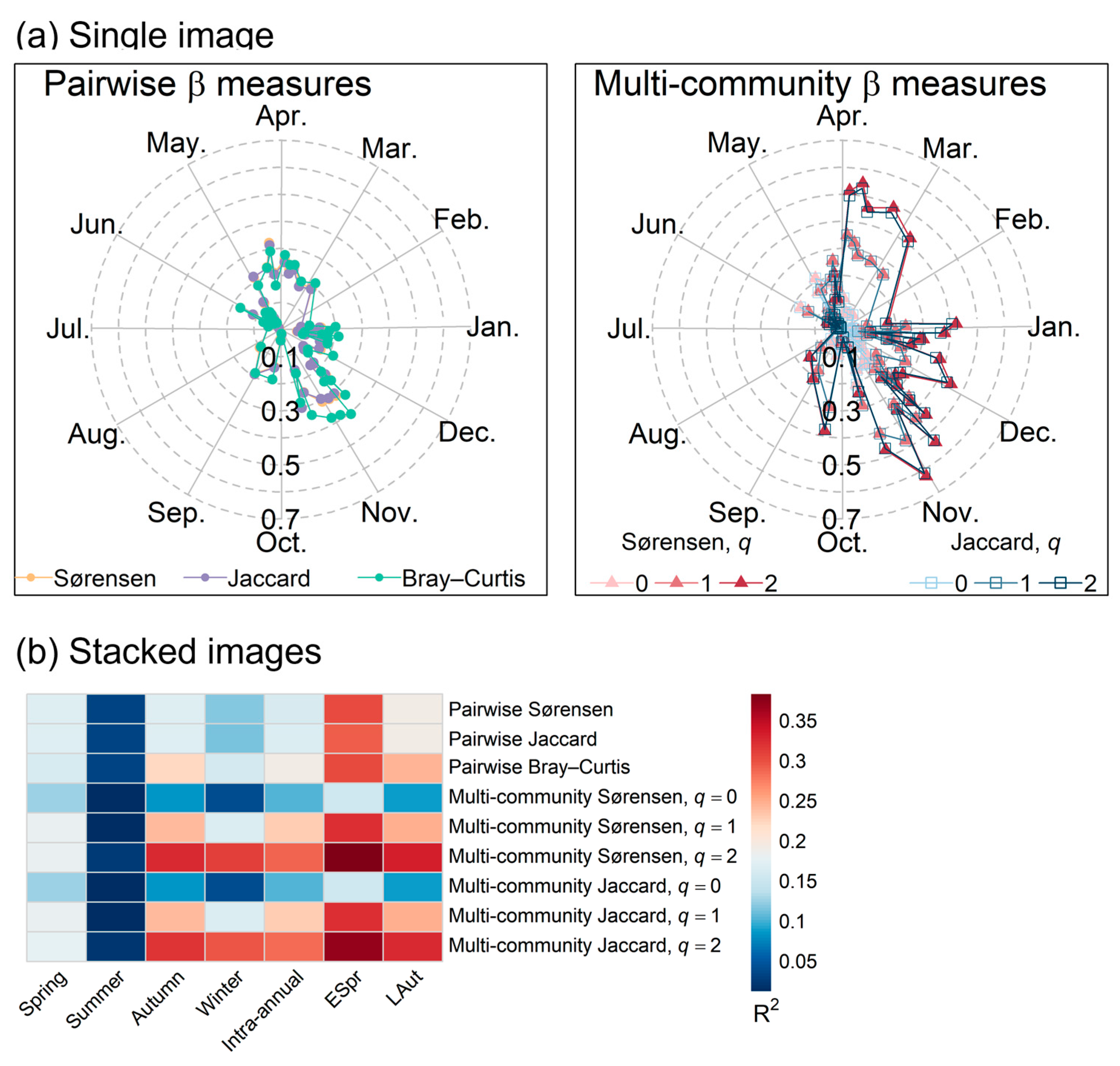
2.3. Strength of Association Between Spectral and Inventory β Diversities

To assess the strength of the association between the spectral and inventory β diversities, we simulated a sampling process by randomly selecting subsets of the 58 field plots to form pooled assemblages. This simulation was repeated 1000 times to generate different pooled assemblages. For each pooled assemblage, we calculated a set of indices of the inventory β diversity and a spectral β index (see below). The coefficient of determination (R2) for simple linear regressions between the spectral β index and each inventory β index across the 1000 repetitions was used to quantify the strength of their association. Recognizing that the β diversity, as a composite concept, is influenced by factors such as the species spatial aggregation, species pool size, and species abundance distribution [6,42], we also calculated a standardized β deviation for each β measure using a randomization-based null model to isolate the spatial component of the β diversity [6]. The strength of the association between the spectral and inventory β deviations was similarly quantified using the coefficient of determination. To assess the robustness of our results, we tested different sample sizes (i.e., the number of local communities in a pooled assemblage, N = 5, 10, 15, 20, 25, 30, 35, 40, 45, and 50) and found that the strength of the association initially increased and then plateaued with an increasing sample size (Figure S2). Therefore, we report the results for N = 40 in the main text.
The spectral β diversity was quantified using the framework developed by Laliberté et al. [33], which measures the spectral diversity as the spectral variance of the 3-D reflectance data cube and additively partitions the overall (γ) spectral diversity of a pooled assemblage into α (within local communities) and β (among local communities) components, following the spirit of a classical analysis of variance (ANOVA). Following the recommendation of Laliberté et al. [33], for each reflectance data cube, we performed a principal component analysis (PCA) with type-I scaling to reduce the data dimensionality, selecting the leading principal components (PCs) that explained up to 99% of the total spectral variation to calculate the spectral diversities. This was first performed for each individual image and then for stacked images comprising images from different seasons within a year (i.e., from March to May for spring, June to August for summer, September to November for autumn, and December to February for winter) or comprising all the images taken within a year. Since the spectral β diversity calculated from the single images acquired in early spring and late autumn showed a stronger association with the inventory β diversity, we also produced two additional stacked images representing early spring (March to April) and late autumn (October to November) to assess whether these could provide better predictions of the β diversity than the single images.
We evaluated the effectiveness of using the spectral β diversity in predicting two sets of widely used β measures calculated from the inventory data. The first set was the averages of dissimilarity indices over all the pairwise local communities within a pooled assemblage, including the Sørensen, Jaccard, and Bray–Curtis indices. These indices are of the same type as the spectral β index described above, as all of them essentially quantify the β diversity using the variance among local communities [33,43]. The second set included six multi-community differentiation measures based on Hill numbers. Three Sørensen-type measures quantified the effective average proportion of a local community’s species not shared across all the communities, with values of q = 0, 1, and 2 representing different weights for the species abundance [44]. Three Jaccard-type measures quantified the effective average proportion of the pooled assemblage’s species not shared across all the local communities, with values of q = 0, 1, and 2 having the same meaning as above. These six measures unify many classical measures of β diversity. For instance, the Jaccard-type measure with a value of q = 0 is simply the widely used “proportional species turnover” metric [45], a monotonic transformation of Whittaker’s multiplicative β [1].
We used the null model proposed by Kraft et al. [6] to calculate the inventory β deviation. For each pooled assemblage, we randomly shuffled all individuals while preserving the abundance of each species and the number of individuals in each local community. From 999 iterations of the null model, we calculated the inventory β deviation for each of the nine inventory β indices as the difference between the observed and mean expected β diversity, divided by the standard deviation of the expected β diversity. We then extended this null model to calculate the spectral β deviation by randomly shuffling the spatial locations of all the pixels in a pooled assemblage. The randomization was repeated 999 times to obtain the spectral β deviation using a similar method as that for obtaining the inventory β deviation (i.e., (observed − mean)/(SD)).

2.4. Scale-Dependent Elevational Gradient of Spectral β Diversity

All the analyses described in this section were based on the Sentinel-2 image acquired on 31 October 2019, which provided one of the best predictions of the inventory β diversities. We also tested several other images that performed similarly in predicting the inventory β diversity, and the results were qualitatively similar (Figures S3 and S4), indicating robustness to the choice of images. The image was divided into a grid of 20 × 20 m cells, corresponding to the scale of the local communities for which we had collected field data. The cells were then grouped into “landscape units” with equal areas using a neighboring, non-overlapping principle, where each cell belonged to only one landscape unit, and nearby cells were grouped into the same landscape unit (Figure S5). For each landscape unit, the spectral β diversity was calculated following the same procedure as described in the previous section. To investigate the scale dependence in the elevational gradient of the spectral β diversity, we considered 11 different spatial extents when defining the landscape units, ranging from 0.16 ha (4 cells of 20 × 20 m) to 64 ha (Figure S5). Local communities where not all the constituent pixels were classified as vegetation were excluded, and the remaining local communities were used to calculate the spectral β diversity for each landscape unit.
For the analysis of topographic variables, we used a Digital Elevation Model (DEM) derived from Advanced Land Observing Satellite/Phased Array type-L band Synthetic Aperture Radar (ALOS/PALSAR) data acquired on 3 January 2008 with a spatial resolution of 12.5 m. Three topographic variables were calculated: the elevation, slope, and aspect. The aspect values were sine- and cosine-transformed to represent the eastness and northness, respectively. The standard deviation was calculated for each topographic variable for each landscape unit generated as described above.
We used partial regressions to partition the variation in the β diversity for each spatial extent into four components: (a) variation uniquely explained by the elevation, (b) variation jointly explained by the elevation and topographic heterogeneity, (c) variation uniquely explained by the topographic heterogeneity, and (d) the unexplained portion. The proportion of the variation explained by the topographic heterogeneity was further partitioned into the portions of the variation explained by different variables. The mean elevation of each landscape unit, together with its quadratic and cubic terms, addressing the visually observable nonlinear patterns, was used to model the elevational patterns. The variables representing the topographic heterogeneity included the standard deviation of the elevation, slope, and sine- and cosine-transformed aspect values for a landscape unit. The local variation in the elevation and eastness exhibited a negligible contribution to the spectral β diversity across all the spatial extents. Thus, the results of the variation partitioning presented in the main text only incorporate the standard deviation of the slope and northness as variables representing the topographic heterogeneity.
All statistical analyses were conducted in R version 4.0.5 (R Core Team, 2021) [46].

3. Results

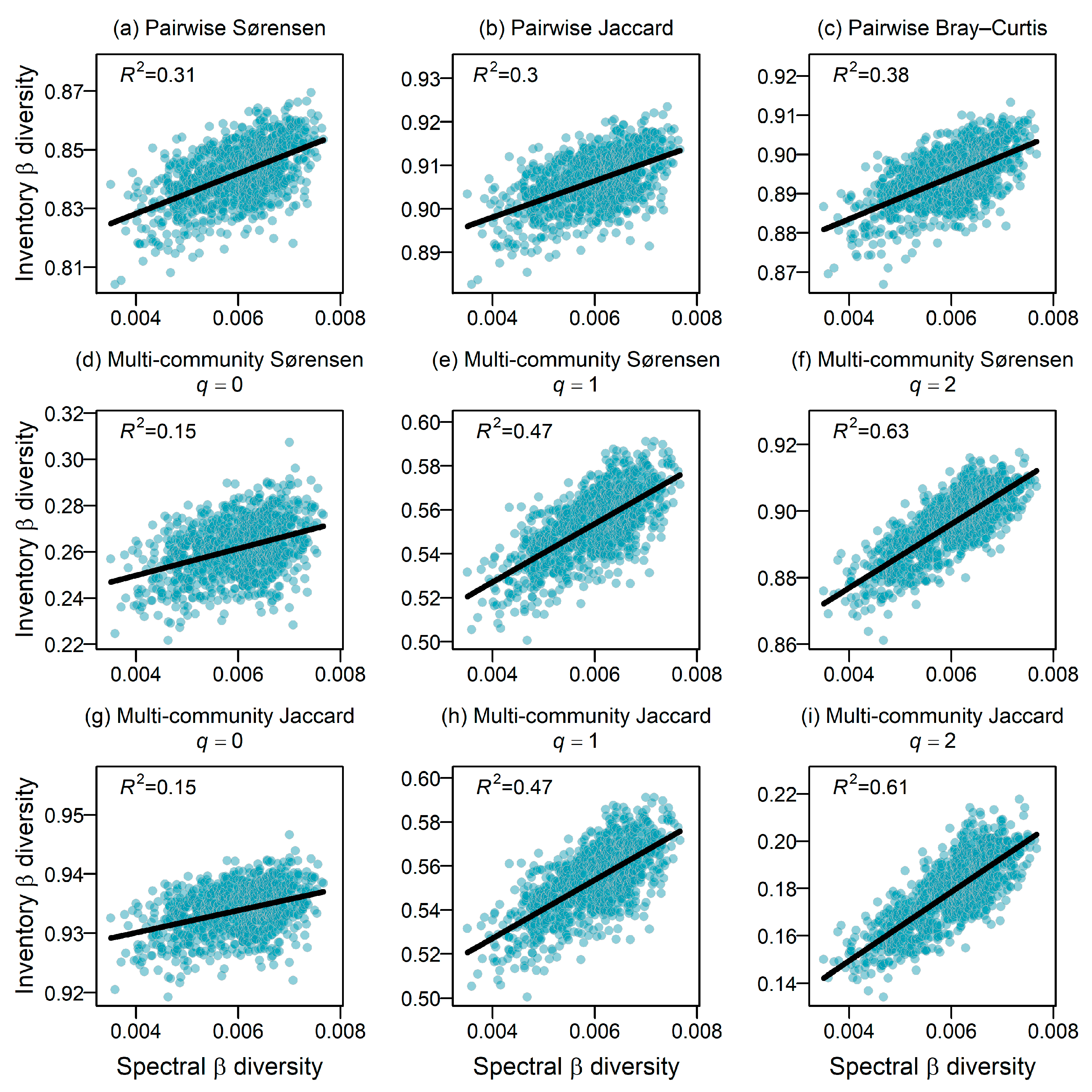
3.1. Strength of Association Between Spectral and Inventory β Diversity

The spectral β diversity was an effective predictor of the inventory β diversity, although the strength of this relationship varied by the season. The strongest correlations between the spectral and inventory β diversity indices were observed in single images acquired in early spring (March to April) and late autumn (October to November) (Figure 1a). This pattern was consistent across various combinations of stacked images (Figure 1b and Figure S6).
The association between the spectral and inventory β diversity also varied depending on the type of inventory β diversity index used. The spectral β diversity was more strongly correlated with abundance-based β indices (Figure 2, average R2 = 0.51 for the best-performing image) compared to occurrence-based β indices (average R2 = 0.23). Multi-community differentiation measures with a value of q = 2 showed the strongest association with the spectral β diversity (R2 = 0.63 for the Sørensen-type measure and R2 = 0.61 for the Jaccard-type measure). In contrast, the spectral β deviation did not perform well in predicting the inventory β deviation indices (Figure 3).

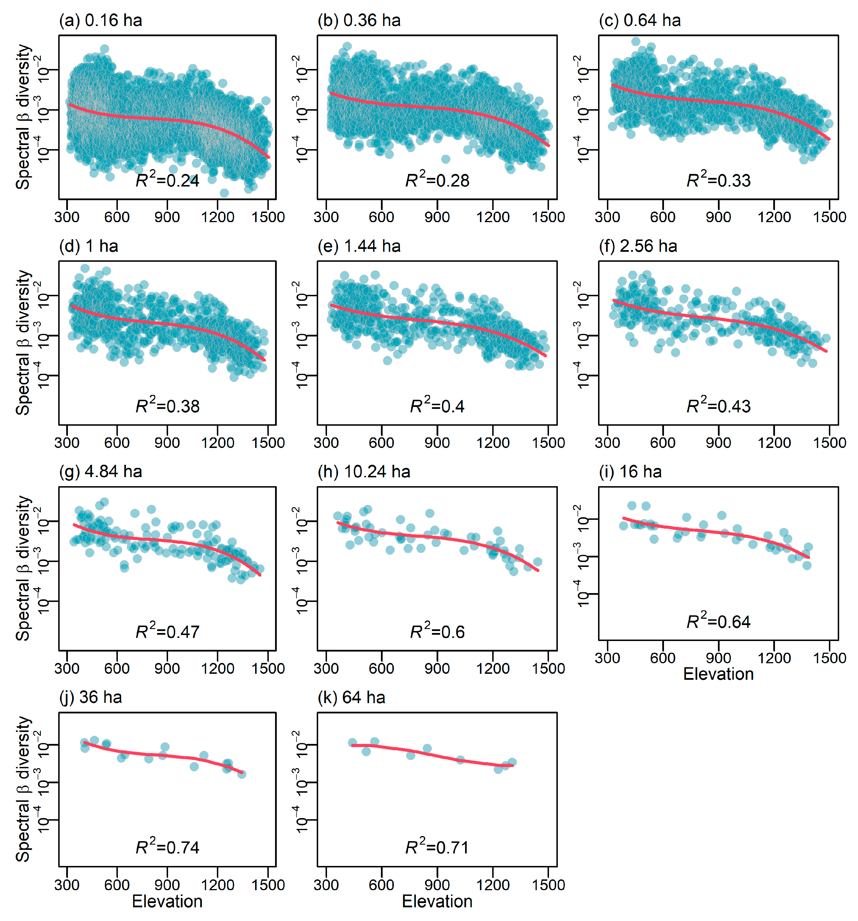
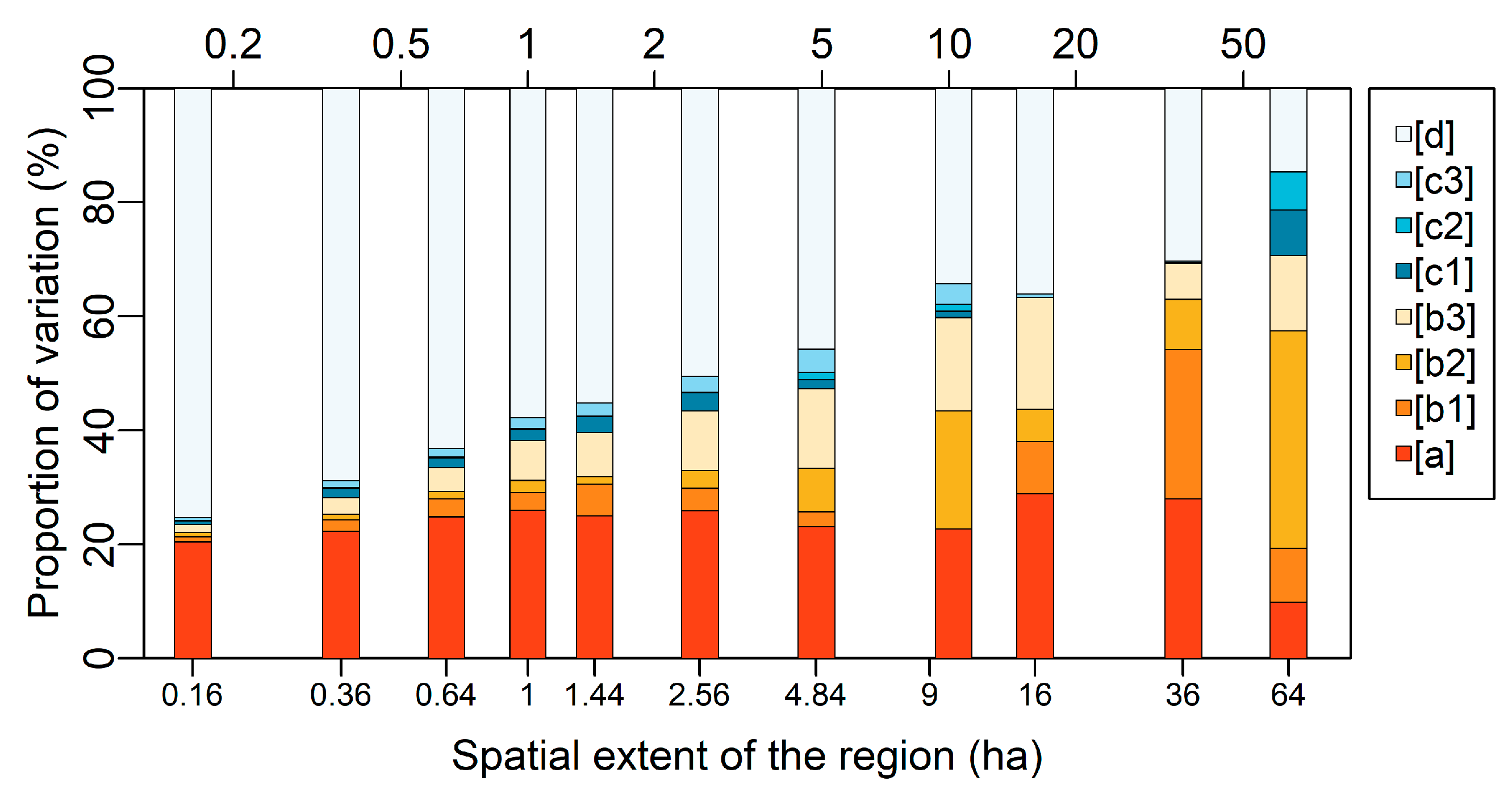
3.2. Scale-Dependent Elevational Patterns and Drivers of Spectral β Diversity

The spectral β diversity consistently decreased with the elevation across all the studied spatial extents, although this relationship was nonlinear (Figure 4). The strength of the relationship increased with larger spatial extents, with the R2 values ranging from 0.24 at 0.16 ha to 0.71 at 64 ha (Figure 4). One could argue that the observed strengthening of the relationship between the spectral β diversity and elevation with an increasing spatial extent was an artifact due to the reduced sample size at broader spatial extents. However, this is not true. For instance, randomly subsampling 10 data points from Figure 4a, each representing the spectral β diversity calculated for a landscape unit of 0.16 ha, to refit the trend resulted in an association of a similar strength, as reported in the figure (the mean adjusted R2 and 95% CI from 100 repetitions were 0.14 and −0.16 to 0.35). Therefore, the increase in the R2 with the spatial extent cannot be attributed to the decrease in the sample size. The elevation and topographic heterogeneity together explained 24% to 85% of the variation in the spectral β diversity across the spatial extents examined (Figure 5). Approximately 20% of the variation in the spectral β diversity at all extents was attributed uniquely to the elevation.
The increased strength of the elevational gradient in the spectral β diversity at larger spatial extents was primarily driven by the topographic heterogeneity, represented by the slope and northness. Their contribution, along with that of the elevation, to the spectral β diversity increased from ~3% at the smallest extent (0.16 ha) to over 50% at the largest extent (64 ha). For about half of this proportion, the variation explained ([b3] in Figure 5) was indistinguishable between the slope and northness. At smaller spatial extents (0.16–2.56 ha), the unique contribution of the northness to the elevational gradient ([b1] in Figure 5) was greater than that of the slope, while the slope became more influential at larger extents (4.84–64 ha). The unique contribution of the topographic heterogeneity, independent of the elevation, was negligible across all the spatial extents.

4. Discussion

The scale dependence of β diversity patterns along latitudinal and altitudinal gradients has been well established. Recent studies have emphasized the role of environmental heterogeneity in shaping patterns of β diversity, especially over broad spatial extents. However, its role at smaller spatial scales is debated, and the threshold beyond which the effect of environmental heterogeneity becomes detectable remains uncertain. In this study, we leveraged remote sensing data to address these gaps.

4.1. Strength of Association Between Spectral and Inventory β Diversity

Our study demonstrated that Sentinel-2 multispectral imagery effectively predicted the canopy tree β diversity, though this predictability varied with both the season of data acquisition and the type of β diversity index used. We found that the spectral β diversity from images captured in early spring and late autumn exhibited the strongest correlations with the inventory β diversity. This suggests that interspecific phenological differences are key in linking remote sensing data with biodiversity patterns, particularly in ecosystems with pronounced seasonality [25,26,47,48,49,50]. These results align with previous findings that remote sensing data from the start and end of growing seasons [25,51,52] best predict plant diversity. The study region is characterized by mixed evergreen and deciduous broad-leaved forests. During these transitional seasons, phenological asynchronies, such as differences in the timing of sprouting, flowering, greening, and defoliating, can enhance the detection of interspecific differences in the canopy tree species [48,49,53]. For example, some species may sprout, flower, or lose their leaves earlier than others, leading to distinctly different chlorophyll absorption rates, water moisture, and leaf biomass among species [54]. By contrast, the peak greenness in summer leads to reduced spectral variation among species, limiting the ability of multispectral channels to capture biodiversity signals. The poor performance of winter imagery may be attributed to the characteristics of the study region, which is dominated by a mix of evergreen and deciduous broad-leaved forests. Deciduous species have already shed their leaves during winter, which hinders the ability of remote sensing data to effectively capture the spectral variation of these species. However, it should be noted that the seasonal dependence of the relationship between the spectral diversity and tree diversity may also rely on the ecosystem. For example, Maeda et al. [55] demonstrated that the relationship between remote sensing data and plant diversity depended on the precipitation patterns in Kenya, with greater predictive power observed when using imagery from the dry season but a weak correlation for the wet season imagery.
It is no surprise that the spectral β diversity correlated more strongly with abundance-based inventory β indices than with occurrence-based indices. This parallels earlier work on α diversity, where abundance-weighted α metrics like Shannon’s and Simpson’s metrics were found to be more reliably predicted from remote sensing data than the species richness [23,25,26,56,57]. The multi-community β diversity measures with a value of q = 2 showed the strongest correlation with the spectral β diversity, likely because these indices place more emphasis on common species. The spectral β diversity measure used in this study, like many other spectral diversity indices, treated each individual, not species, equally. Future studies may develop and test new spectral β diversity measures that take into account uneven species abundance distributions, if the aim is to predict the incidence-based β diversity.
While β deviation metrics are frequently used to isolate the spatial aggregation component of the β diversity [6,42], our spectral β deviation, based on randomized pixel shuffling, had only a weak relationship with the inventory-based β deviation. This was likely due to a mismatch in the spatial scale: remote sensing pixels represent 10 × 10 m areas, containing an average of 12 (range: 3–50) individual trees in our dataset. As such, the spectral β deviation failed to incorporate spatial aggregation at scales smaller than 10 m, including a major range of scales at which strong spatial aggregation is often detected for tree species [58]. High-resolution (e.g., UAV-based) imagery or hyperspectral remote sensing technology can be incorporated in the future to further evaluate the potential of remote sensing in capturing the β deviation.

4.2. Scale-Dependent Spatial Patterns and Drivers of Spectral β Diversity Along Elevation Gradient

Our study confirmed that the spectral β diversity decreased with the elevation, a pattern consistent with previous research based on inventory data [6,11,15,59]. However, these earlier studies were often limited to a single or few arbitrary sampling extents, leaving questions regarding the role of environmental filtering unresolved. By leveraging the continuous nature of satellite remote sensing data, we revealed that the association between the topographic heterogeneity and spectral β diversity strengthened as the spatial extent increased. This association contributed more than 50% to explaining the elevational gradient of the spectral β diversity for spatial extents as small as 4 ha, highlighting the significant role of environmental filtering in shaping the canopy tree distribution along an elevational gradient.
Our results further identified two local topographic features, the slope and northness, as drivers of the β diversity. Interestingly, the relative importance of these factors was scale-dependent. At smaller spatial extents (0.16–2.56 ha), the northness emerged as the dominant factor, likely due to the pronounced effects of microclimatic variation. The differential exposure to light, temperatures, and moisture between north- and south-facing slopes creates distinct ecological niches. For instance, south-facing slopes, being warmer and drier, support sun-tolerant, drought-resistant species, while cooler, more humid north-facing slopes favor shade-tolerant species [60]. This microclimatic variation explains the observed influence of the northness on the tree community structure at finer spatial scales [61].
As the spatial extent increased, the slope overtook the northness as the more important driver of the β diversity. This shift may have been linked to the soil nutrient distribution, as steeper slopes often experience erosion and nutrient runoff, leading to poorer soil conditions. Previous studies [36,62,63] have demonstrated that the slope significantly affects species distributions, particularly at larger spatial scales, where soil nutrient variation becomes more pronounced. Our results align with this perspective, suggesting that the slope is a key factor shaping the tree community composition at broader spatial extents. We note that the topographic variables used in this study were derived from ALOS/PALSAR data, which may have been affected by the canopy height and biased our estimation of the contribution of these variables. Nevertheless, the spatial extent of the landscape units analyzed in this study was mostly much greater than the typical canopy height in the study region, suggesting that the influence of this may not have been large. Future studies could use more accurate digital terrain model products such as those derived using LiDAR techniques to confirm our findings.
The influence of the topographic heterogeneity on the spectral β diversity became negligible at fine scales but significantly increased at broader scales. This scale threshold is consistent with findings from previous studies. Mori et al. [15] showed a positive correlation between the β diversity at spatial extent of about 400 m and the elevation, suggesting effects from local processes. Tello et al. [11] found that local processes play a negligible role in shaping the elevational gradients of the β diversity at an extent of 50 m but contribute significantly to explaining the β diversity at an extent of 19 km. Our study advanced this understanding by utilizing continuous spatial data, demonstrating that the effect of the topographic heterogeneity began to dominate the spectral β diversity at extents as small as 4 ha and grew stronger as the spatial extent increased.
We also found that the elevation, independent of other factors, consistently explained about 20% of the variation in the spectral β diversity across all the spatial extents. This unique contribution of the elevation dropped to less than 3% when the spectral γ diversity was included as a predictor (Figure S7). This underscores “the tangled relationship between β and γ diversity” and the importance of considering both in studies of diversity patterns [64]. One approach addressing this is to use the β deviation instead of the raw β diversity. We did not model the spectral β deviation because of its weak correlation with the inventory β deviation. An alternative approach is to include the γ diversity as a predictor when modeling the β diversity [64]. We adopted this approach in our study. The inclusion of the spectral γ diversity as a predictor substantially increased the explained proportion of the variation in the spectral β diversity across all the extents, but it did not alter the scale-dependent contribution of the topographic heterogeneity (Figure S7), suggesting that topographic factors affected the β diversity through the spatial distribution of species, not the total number of species in a landscape unit.

5. Conclusions

In summary, our study showcases the potential of using multispectral satellite remote sensing data to predict the tree β diversity and highlights the scale-dependent nature of its elevational patterns. The spectral β diversity showed a marked decline with an increasing elevation, with the topographic heterogeneity playing a critical role in shaping this gradient, particularly at spatial extents of 4 ha or greater. The slope and northness were identified as key drivers, with their influence varying across spatial scales: the impact of the northness dominated at finer extents, while the slope became more influential at broader extents. While our results shed light on the effectiveness of using remote sensing techniques to address difficult questions relating to plant diversity, we acknowledge that the findings were only derived from one elevational gradient on a subtropical mountain and are far from conclusive. Further research is needed to confirm and generalize our conclusions.
We envisage three ways in which this study could be further refined and extended. First, future studies should consider utilizing high-spatial-resolution imagery (such as airborne hyperspectral data or WorldView-2 satellite imagery) or emerging new remote sensing techniques to enhance the predictive capability for the β diversity and β deviation. Second, although our findings have already shown that remote sensing data could effectively capture the variation in the tree β diversity despite the relatively small number of field survey plots, we acknowledge that a larger sample size could be very helpful in improving the model’s robustness and predictive power. Third, future studies should aim to disentangle the relative contributions of other environmental factors, such as soil nutrients and microclimates, while expanding the analysis to larger spatial scales and different ecosystems to provide a more comprehensive understanding of β diversity patterns.

Supplementary Materials

The following supporting information can be downloaded at https://www.mdpi.com/article/10.3390/f16060917/s1: Figure S1: Locations of the field plots in the National Natural Reserve of Tianmu Mountain, Zhejiang, China; Figure S2: Relationship between coefficient of determination (R2) for spectral and inventory β diversities and sample sizes; Figure S3: Elevational trends in spectral β diversity across different spatial extents, derived from single image acquired on 10 November 2019; Figure S4: Proportions of variation in spectral β diversity explained by elevation and topographic heterogeneity for regions at different spatial extents, derived from single image acquired on 10 November 2019; Figure S5: Methods for generating regions for β diversity mapping; Figure S6: Season-dependent association between various indices of inventory β diversity and spectral β diversity; Figure S7: Proportions of variation in spectral β diversity explained by elevation, spectral γ diversity, and topographic heterogeneity for regions at different spatial extents; Table S1: Spectral information of the 10 Sentinel-2A bands used in this study; Table S2: Selection of Sentinel-2 images taken from 2019 to 2022 used in this paper.

Author Contributions

Conceptualization, R.Z., J.Z., and D.X.; formal analysis, R.Z.; investigation, R.Z., J.H., Y.L. (Yongchao Liu), X.W. (Xiaoning Wang), Y.L. (You Li), Y.Z., P.L., X.W. (Xiaoran Wang), Z.Z., J.Z. and D.X.; writing—original draft preparation, R.Z.; writing—review and editing, J.Z. and D.X.; supervision, D.X.; funding acquisition, J.Z. and D.X. All authors have read and agreed to the published version of the manuscript.

Funding

This study was supported by the National Natural Science Foundation of China (32101280 and 32471623) and the Innovation Program of Shanghai Municipal Education Commission (2023ZKZD36).

Data Availability Statement

All the data supporting the results are presented in the main text and Supplementary Materials. The raw remote sensing data are in the public domain. The raw field inventory data are available from the corresponding author.

Acknowledgments

This work was part of the BEST (Biodiversity along Elevational Gradients: Shifts and Transitions; https://BEST-mountains.org) research project.

Conflicts of Interest

The authors declare no conflicts of interest.

References

  1. Whittaker, R.H. Vegetation of the Siskiyou Mountains, Oregon and California. Ecol. Monogr. 1960, 30, 279–338. [Google Scholar] [CrossRef]
  2. Dornelas, M.; Gotelli, N.J.; McGill, B.; Shimadzu, H.; Moyes, F.; Sievers, C.; Magurran, A.E. Assemblage time series reveal biodiversity change but not systematic loss. Science 2014, 344, 296–299. [Google Scholar] [CrossRef] [PubMed]
  3. Mori, A.S.; Isbell, F.; Seidl, R. β-diversity, community assembly, and ecosystem functioning. Trends Ecol. Evol. 2018, 33, 549–564. [Google Scholar] [CrossRef]
  4. Blowes, S.A.; McGill, B.; Brambilla, V.; Chow, C.F.Y.; Engel, T.; Fontrodona-Eslava, A.; Martins, I.S.; McGlinn, D.; Moyes, F.; Sagouis, A.; et al. Synthesis reveals approximately balanced biotic differentiation and homogenization. Sci. Adv. 2024, 10, eadj9395. [Google Scholar] [CrossRef]
  5. Qian, H.; Ricklefs, R.E. A latitudinal gradient in large-scale beta diversity for vascular plants in North America. Ecol. Lett. 2007, 10, 737–744. [Google Scholar] [CrossRef] [PubMed]
  6. Kraft, N.J.; Comita, L.S.; Chase, J.M.; Sanders, N.J.; Swenson, N.G.; Crist, T.O.; Stegen, J.C.; Vellend, M.; Boyle, B.; Anderson, M.J.; et al. Disentangling the drivers of beta diversity along latitudinal and elevational gradients. Science 2011, 333, 1755–1758. [Google Scholar] [CrossRef]
  7. Xing, D.; He, F. Environmental filtering explains a U-shape latitudinal pattern in regional beta-deviation for eastern North American trees. Ecol. Lett. 2019, 22, 284–291. [Google Scholar] [CrossRef]
  8. Cao, K.; Condit, R.; Mi, X.; Chen, L.; Ren, H.; Xu, W.; Burslem, D.; Cai, C.; Cao, M.; Chang, L.; et al. Species packing and the latitudinal gradient in beta-diversity. Proc. R. Soc. B Biol. Sci. 2021, 288, 20203045. [Google Scholar] [CrossRef]
  9. Nishizawa, K.; Shinohara, N.; Cadotte, M.W.; Mori, A.S. The latitudinal gradient in plant community assembly processes: A meta-analysis. Ecol. Lett. 2022, 25, 1711–1724. [Google Scholar] [CrossRef]
  10. Shinohara, N.; Kobayashi, Y.; Nishizawa, K.; Kadowaki, K.; Yamawo, A. Plant–mycorrhizal associations may explain the latitudinal gradient of plant community assembly. Oikos 2024, 2024, e10367. [Google Scholar] [CrossRef]
  11. Tello, J.S.; Myers, J.A.; Macia, M.J.; Fuentes, A.F.; Cayola, L.; Arellano, G.; Loza, M.I.; Torrez, V.; Cornejo, M.; Miranda, T.B.; et al. Elevational gradients in β-diversity reflect variation in the strength of local community assembly mechanisms across spatial scales. PLoS ONE 2015, 10, e0121458. [Google Scholar] [CrossRef] [PubMed]
  12. Zhang, C.; He, F.; Zhang, Z.; Zhao, X.; von Gadow, K. Latitudinal gradients and ecological drivers of β-diversity vary across spatial scales in a temperate forest region. Glob. Ecol. Biogeogr. 2020, 29, 1257–1264. [Google Scholar] [CrossRef]
  13. Liu, M.; Wu, W.; Wang, K.; Ren, X.; Zhang, X.; Wang, L.; Geng, J.; Yang, B. Latitudinal patterns of tree β-diversity and relevant ecological processes vary across spatial extents in forests of southeastern China. Plant Divers. 2025, 47, 89–97. [Google Scholar] [CrossRef]
  14. De Cáceres, M.; Legendre, P.; Valencia, R.; Cao, M.; Chang, L.W.; Chuyong, G.; Condit, R.; Hao, Z.; Hsieh, C.F.; Hubbell, S.; et al. The variation of tree beta diversity across a global network of forest plots. Glob. Ecol. Biogeogr. 2012, 21, 1191–1202. [Google Scholar] [CrossRef]
  15. Mori, A.S.; Shiono, T.; Koide, D.; Kitagawa, R.; Ota, A.T.; Mizumachi, E. Community assembly processes shape an altitudinal gradient of forest biodiversity. Glob. Ecol. Biogeogr. 2013, 22, 878–888. [Google Scholar] [CrossRef]
  16. Qian, H.; Chen, S.; Mao, L.; Ouyang, Z. Drivers of β-diversity along latitudinal gradients revisited. Glob. Ecol. Biogeogr. 2013, 22, 659–670. [Google Scholar] [CrossRef]
  17. Xu, W.; Chen, G.; Liu, C.; Ma, K. Latitudinal differences in species abundance distributions, rather than spatial aggregation, explain beta-diversity along latitudinal gradients. Glob. Ecol. Biogeogr. 2015, 24, 1170–1180. [Google Scholar] [CrossRef]
  18. Martínez-Villa, J.A.; González-Caro, S.; Duque, Á. The importance of grain and cut-off size in shaping tree beta diversity along an elevational gradient in the northwest of Colombia. For. Ecosyst. 2020, 7, 2. [Google Scholar] [CrossRef]
  19. Brinck, K.; Fischer, R.; Groeneveld, J.; Lehmann, S.; Dantas De Paula, M.; Pütz, S.; Sexton, J.O.; Song, D.; Huth, A. High resolution analysis of tropical forest fragmentation and its impact on the global carbon cycle. Nat. Commun. 2017, 8, 14855. [Google Scholar] [CrossRef]
  20. Cavender-Bares, J.; Gamon, J.A.; Townsend, P.A. Remote Sensing of Plant Biodiversity; Springer Nature: Cham, Switzerland, 2020. [Google Scholar]
  21. Wang, R.; Gamon, J.A. Remote sensing of terrestrial plant biodiversity. Remote Sens. Environ. 2019, 231, 111218. [Google Scholar] [CrossRef]
  22. Cavender-Bares, J.; Schneider, F.D.; Santos, M.J.; Armstrong, A.; Carnaval, A.; Dahlin, K.M.; Fatoyinbo, L.; Hurtt, G.C.; Schimel, D.; Townsend, P.A.; et al. Integrating remote sensing with ecology and evolution to advance biodiversity conservation. Nat. Ecol. Evol. 2022, 6, 506–519. [Google Scholar] [CrossRef]
  23. Wang, R.; Gamon, J.A.; Schweiger, A.K.; Cavender-Bares, J.; Townsend, P.A.; Zygielbaum, A.I.; Kothari, S. Influence of species richness, evenness, and composition on optical diversity: A simulation study. Remote Sens. Environ. 2018, 211, 218–228. [Google Scholar] [CrossRef]
  24. Schweiger, A.K.; Laliberté, E. Plant beta-diversity across biomes captured by imaging spectroscopy. Nat. Commun. 2022, 13, 2767. [Google Scholar] [CrossRef]
  25. Liu, Y.; Zhang, R.; Lin, C.; Zhang, Z.; Zhang, R.; Shang, K.; Zhao, M.; Huang, J.; Wang, X.; Li, Y.; et al. Remote sensing of subtropical tree diversity: The underappreciated roles of the practical definition of forest canopy and phenological variation. For. Ecosyst. 2023, 10, 100122. [Google Scholar] [CrossRef]
  26. Liu, X.; Frey, J.; Munteanu, C.; Still, N.; Koch, B. Mapping tree species diversity in temperate montane forests using Sentinel-1 and Sentinel-2 imagery and topography data. Remote Sens. Environ. 2023, 292, 113576. [Google Scholar] [CrossRef]
  27. Chen, B.J.; Teng, S.N.; Zheng, G.; Cui, L.; Li, S.; Staal, A.; Eitel, J.U.; Crowther, T.W.; Berdugo, M.; Mo, L.; et al. Inferring plant–plant interactions using remote sensing. J. Ecol. 2022, 110, 2268–2287. [Google Scholar] [CrossRef]
  28. He, K.S.; Zhang, J.; Zhang, Q. Linking variability in species composition and MODIS NDVI based on beta diversity measurements. Acta Oecol. 2009, 35, 14–21. [Google Scholar] [CrossRef]
  29. Dalmayne, J.; Möckel, T.; Prentice, H.C.; Schmid, B.C.; Hall, K. Assessment of fine-scale plant species beta diversity using WorldView-2 satellite spectral dissimilarity. Ecol. Inform. 2013, 18, 1–9. [Google Scholar] [CrossRef]
  30. Van Der Meer, F.; Bakker, W.; Scholte, K.; Skidmore, A.; De Jong, S.; Clevers, J.; Addink, E.; Epema, G. Spatial scale variations in vegetation indices and above-ground biomass estimates: Implications for MERIS. Int. J. Remote Sens. 2001, 22, 3381–3396. [Google Scholar] [CrossRef]
  31. Ma, X.; Mahecha, M.D.; Migliavacca, M.; van der Plas, F.; Benavides, R.; Ratcliffe, S.; Kattge, J.; Richter, R.; Musavi, T.; Baeten, L.; et al. Inferring plant functional diversity from space: The potential of Sentinel-2. Remote Sens. Environ. 2019, 233, 111368. [Google Scholar] [CrossRef]
  32. Féret, J.B.; Asner, G.P. Mapping tropical forest canopy diversity using high-fidelity imaging spectroscopy. Ecol. Appl. 2014, 24, 1289–1296. [Google Scholar] [CrossRef] [PubMed]
  33. Laliberté, E.; Schweiger, A.K.; Legendre, P. Partitioning plant spectral diversity into alpha and beta components. Ecol. Lett. 2020, 23, 370–380. [Google Scholar] [CrossRef] [PubMed]
  34. Draper, F.C.; Baraloto, C.; Brodrick, P.G.; Phillips, O.L.; Martinez, R.V.; Honorio Coronado, E.N.; Baker, T.R.; Zárate Gómez, R.; Amasifuen Guerra, C.A.; Flores, M.; et al. Imaging spectroscopy predicts variable distance decay across contrasting Amazonian tree communities. J. Ecol. 2019, 107, 696–710. [Google Scholar] [CrossRef]
  35. Opedal, Ø.H.; Armbruster, W.S.; Graae, B.J. Linking small-scale topography with microclimate, plant species diversity and intra-specific trait variation in an alpine landscape. Plant Ecol. Divers. 2015, 8, 305–315. [Google Scholar] [CrossRef]
  36. John, R.; Dalling, J.W.; Harms, K.E.; Yavitt, J.B.; Stallard, R.F.; Mirabello, M.; Hubbell, S.P.; Valencia, R.; Navarrete, H.; Vallejo, M.; et al. Soil nutrients influence spatial distributions of tropical tree species. Proc. Natl. Acad. Sci. USA 2007, 104, 864–869. [Google Scholar] [CrossRef]
  37. Jiang, X.; Zhang, X. Comprehensive Investigation Report on Natural Resource of Tianmu Mountain Nature Reserve; Zhejiang Science and Technology Press: Hangzhou, China, 1992. (In Chinese) [Google Scholar]
  38. Da, L.; Kang, M.; Song, K.; Shang, K.; Yang, Y.; Xia, A.; Qi, Y. Altitudinal zonation of human-disturbed vegetation on Mt. Tianmu, eastern China. Ecol. Res. 2009, 24, 1287–1299. [Google Scholar] [CrossRef]
  39. Zhang, R.; Zhang, Z.; Shang, K.; Zhao, M.; Kong, J.; Wang, X.; Wang, Y.; Song, H.; Zhang, O.; Lv, X.; et al. A taxonomic and phylogenetic perspective on plant community assembly along an elevational gradient in subtropical forests. J. Plant Ecol. 2021, 14, 702–716. [Google Scholar] [CrossRef]
  40. Drusch, M.; Del Bello, U.; Carlier, S.; Colin, O.; Fernandez, V.; Gascon, F.; Hoersch, B.; Isola, C.; Laberinti, P.; Martimort, P.; et al. Sentinel-2: ESA’s optical high-resolution mission for GMES operational services. Remote Sens. Environ. 2012, 120, 25–36. [Google Scholar] [CrossRef]
  41. Enache, S. Data Quality Report-Sentinel-2 L1C MSI; No. OMPC. CS. DQR. 01.01-2022; ESA: Paris, France, 2022. [Google Scholar]
  42. Xing, D.; He, F. Analytical models for β-diversity and the power-law scaling of β-deviation. Methods Ecol. Evol. 2021, 12, 405–414. [Google Scholar] [CrossRef]
  43. Legendre, P.; De Cáceres, M. Beta diversity as the variance of community data: Dissimilarity coefficients and partitioning. Ecol. Lett. 2013, 16, 951–963. [Google Scholar] [CrossRef]
  44. Chao, A.; Chiu, C.H. Bridging the variance and diversity decomposition approaches to beta diversity via similarity and differentiation measures. Methods Ecol. Evol. 2016, 7, 919–928. [Google Scholar] [CrossRef]
  45. Tuomisto, H. A diversity of beta diversities: Straightening up a concept gone awry. Part 1. Defining beta diversity as a function of alpha and gamma diversity. Ecography 2010, 33, 2–22. [Google Scholar] [CrossRef]
  46. R Core Team. R: A Language and Environment for Statistical Computing; Version 4.0.5; R Foundation for Statistical Computing: Vienna, Australia, 2021. [Google Scholar]
  47. Kollert, A.; Bremer, M.; Löw, M.; Rutzinger, M. Exploring the potential of land surface phenology and seasonal cloud free composites of one year of Sentinel-2 imagery for tree species mapping in a mountainous region. Int. J. Appl. Earth Obs. Geoinf. 2021, 94, 102208. [Google Scholar] [CrossRef]
  48. Dronova, I.; Taddeo, S. Remote sensing of phenology: Towards the comprehensive indicators of plant community dynamics from species to regional scales. J. Ecol. 2022, 110, 1460–1484. [Google Scholar] [CrossRef]
  49. Wang, R.; Gamon, J.A.; Cavender-Bares, J. Seasonal patterns of spectral diversity at leaf and canopy scales in the Cedar Creek prairie biodiversity experiment. Remote Sens. Environ. 2022, 280, 113169. [Google Scholar] [CrossRef]
  50. Jiang, M.; Kong, J.; Zhang, Z.; Hu, J.; Qin, Y.; Shang, K.; Zhao, M.; Zhang, J. Seeing Trees from Drones: The Role of Leaf Phenology Transition in Mapping Species Distribution in Species-Rich Montane Forests. Forests 2023, 14, 908. [Google Scholar] [CrossRef]
  51. Madonsela, S.; Cho, M.A.; Ramoelo, A.; Mutanga, O. Investigating the relationship between tree species diversity and landsat-8 spectral heterogeneity across multiple phenological stages. Remote Sens. 2021, 13, 2467. [Google Scholar] [CrossRef]
  52. Thornley, R.; Gerard, F.F.; White, K.; Verhoef, A. Intra-annual taxonomic and phenological drivers of spectral variance in grasslands. Remote Sens. Environ. 2022, 271, 112908. [Google Scholar] [CrossRef]
  53. Zutta, B. Assessing Vegetation Functional Type and Biodiversity in Southern California Using Spectral Reflectance. Ph.D. Thesis, California State University, Los Angeles, CA, USA, 2003. [Google Scholar]
  54. Schriever, J.R.; Congalton, R.G. Evaluating seasonal variability as an aid to cover-type mapping from Landsat Thematic Mapper data in the Northeast. Photogramm. Eng. Remote Sens. 1995, 61, 321–327. [Google Scholar]
  55. Maeda, E.E.; Heiskanen, J.; Thijs, K.W.; Pellikka, P.K. Season-dependence of remote sensing indicators of tree species diversity. Remote Sens. Lett. 2014, 5, 404–412. [Google Scholar] [CrossRef]
  56. Dogan, H.M.; Dogan, M. A new approach to diversity indices–modeling and mapping plant biodiversity of Nallihan (A3-Ankara/Turkey) forest ecosystem in frame of geographic information systems. Biodivers. Conserv. 2006, 15, 855–878. [Google Scholar] [CrossRef]
  57. Oldeland, J.; Wesuls, D.; Rocchini, D.; Schmidt, M.; Jürgens, N. Does using species abundance data improve estimates of species diversity from remotely sensed spectral heterogeity? Ecol. Indic. 2010, 10, 390–396. [Google Scholar] [CrossRef]
  58. Condit, R.; Ashton, P.S.; Baker, P.; Bunyavejchewin, S.; Gunatilleke, S.; Gunatilleke, N.; Hubbell, S.P.; Foster, R.B.; Itoh, A.; LaFrankie, J.V.; et al. Spatial patterns in the distribution of tropical tree species. Science 2000, 288, 1414–1418. [Google Scholar] [CrossRef]
  59. Sabatini, F.M.; Jiménez-Alfaro, B.; Burrascano, S.; Lora, A.; Chytrý, M. Beta-diversity of central European forests decreases along an elevational gradient due to the variation in local community assembly processes. Ecography 2018, 41, 1038–1048. [Google Scholar] [CrossRef]
  60. Cantlon, J.E. Vegetation and microclimates on north and south slopes of Cushetunk Mountain, New Jersey. Ecol. Monogr. 1953, 23, 241–270. [Google Scholar] [CrossRef]
  61. Miura, M.; Manabe, T.; Nishimura, N.; Yamamoto, S.I. Forest canopy and community dynamics in a temperate old-growth evergreen broad-leaved forest, south-western Japan: A 7-year study of a 4-ha plot. J. Ecol. 2001, 89, 841–849. [Google Scholar] [CrossRef]
  62. Comita, L.S.; Condit, R.; Hubbell, S.P. Developmental changes in habitat associations of tropical trees. J. Ecol. 2007, 95, 482–492. [Google Scholar] [CrossRef]
  63. Guo, Y.; Wang, B.; Li, D.; Mallik, A.U.; Xiang, W.; Ding, T.; Wen, S.; Lu, S.; Huang, F.; He, Y.; et al. Effects of topography and spatial processes on structuring tree species composition in a diverse heterogeneous tropical karst seasonal rainforest. Flora 2017, 231, 21–28. [Google Scholar] [CrossRef]
  64. Ulrich, W.; Baselga, A.; Kusumoto, B.; Shiono, T.; Tuomisto, H.; Kubota, Y. The tangley5asd link between β-and γ-diversity: A Narcissus effect weakens statistical inferences in null model analyses of diversity patterns. Glob. Ecol. Biogeogr. 2017, 26, 1–5. [Google Scholar] [CrossRef]
Figure 1. Season-dependent association between various indices of inventory β diversity and spectral β diversity. (a) Coefficient of determination (R2) was calculated from single images. (b) Mean coefficient of determination (R2) across four years (2019, 2020, 2021, and 2022) for various intra-annual combinations of stacked images. Abbreviations: ESpr, early spring; LAut, late autumn.
Forests 16 00917 g001
Figure 2. Relationships between spectral β diversity and various indices of inventory β diversity, derived from one of best-performing single images (31 October 2019). Blue dots show spectral β diversity in each simulated pooled assemblage. Black lines are significant fitted linear regression between spectral β diversity and inventory β diversity. Corresponding R2 for each regression is also shown.
Forests 16 00917 g002
Figure 3. Relationship between spectral β deviation and inventory β deviation across various β indices, derived from one of best-performing single images (31 October 2019). Blue dots show spectral β deviation in each simulated pooled assemblage. Black lines are significant fitted linear regression between spectral β deviation and inventory β deviation. Corresponding R2 for each regression is also shown.
Forests 16 00917 g003
Figure 4. Elevational trends in the spectral β diversity calculated at different spatial extents, derived from one of the best-performing single images (31 October 2019). The blue dots show the spectral β diversity within each landscape unit at different spatial extents. Fitted cubic regression lines with their corresponding R2 values are shown to illustrate the trends.
Forests 16 00917 g004
Figure 5. Proportions of the variation in the spectral β diversity explained by the elevation and topographic heterogeneity for landscape units at different spatial extents, derived from one of the best-performing single images (31 October 2019). [a] Variation explained by the elevation only; [b1] shared variation explained by the elevation and the standard deviation of the northness; [b2] shared variation explained by the elevation and the standard deviation of the slope; [b3] shared variation explained by the elevation, the standard deviation of the northness, and the standard deviation of the slope; [c1] variation explained by the standard deviation of the northness only; [c2] variation explained by the standard deviation of the slope only; [c3] shared variation explained by the standard deviation of the northness and the standard deviation of the slope; [d] unexplained variation.
Forests 16 00917 g005
Table 1. Season of image acquisition and its relation to the vegetation phenology, contributing to the association between the spectral and inventory plant diversity in the study region.
SeasonVegetation Phenology
Early spring (March–April)Bud breaking and initial leaf sprouting
Late spring (May)Leaf expansion and flowering
Summer (June–August)Growing season/peak greenness
Early autumn (September)Initial defoliation
Late autumn (October–November)Leaf senescence and defoliation
Winter (December–February)Dormant phase/evergreen persistence
Disclaimer/Publisher’s Note: The statements, opinions and data contained in all publications are solely those of the individual author(s) and contributor(s) and not of MDPI and/or the editor(s). MDPI and/or the editor(s) disclaim responsibility for any injury to people or property resulting from any ideas, methods, instructions or products referred to in the content.

