Article

Interplay of Topography, Fire History, and Climate on Interior Alaska Boreal Forest Vegetation Dynamics in the 21st Century: A Landsat Time-Series Analysis

1
Institute of Agriculture, Natural Resources and Extension, University of Alaska Fairbanks, Fairbanks, AK 99775, USA
2
Institute of Arctic Biology, University of Alaska Fairbanks, Fairbanks, AK 99775, USA
3
International Arctic Research Center, University of Alaska Fairbanks, Fairbanks, AK 99775, USA
4
State Private & Tribal Forestry, USDA Forest Service, Juneau, AK 99801, USA
*
Author to whom correspondence should be addressed.
Forests 2025, 16(5), 777; https://doi.org/10.3390/f16050777
Submission received: 18 March 2025 / Revised: 27 April 2025 / Accepted: 29 April 2025 / Published: 4 May 2025

Abstract

:
This study investigates vegetation dynamics in boreal forests of Interior Alaska, focusing on topography, fire history, and climate influences. The study area includes Bonanza Creek Experimental Forest (BCEF) and surrounding region, categorized by topography (upland, floodplain, lowland) and fire history. Using Mann–Kendall trend and Theil–Sen slope analyses on Landsat-derived spectral metrics: Normalized Difference Vegetation Index (NDVI) and Normalized Burn Ratio (NBR), we observed a shift from browning to greening trends, particularly in historically burned areas. The photosynthetic activity in burned upland converged with unburned areas ~30 years post-fire, coincident with a shift towards deciduous dominance during post-fire succession. Normalized Difference Moisture Index (NDMI) trends revealed a significant increase in vegetation moisture content across all topographies. We introduce Effective Seasonal Precipitation Index (ESPI), which combines prior-year annual precipitation with current-year spring snow depth. Its positive correlation with NDMI highlights its potential for monitoring vegetation moisture dynamics at the landscape scale. Furthermore, by correlating dendrochronology-based climate indices, we found strong correlation between NDMI and normalized Supplemental Precipitation Index (nSPI), across topographies. Overall, this research provides critical insights into how climate and fire influence interior boreal vegetation, highlighting the effects of increased precipitation, and topography on shaping differential vegetation responses across the landscape.

1. Introduction

Alaska encompasses approximately 51 million hectares of forested land, primarily boreal and coastal temperate forests. The boreal forest covers 60%–70% of the state’s land, stretching across Interior Alaska between the Brooks Range in the north and the Alaska Range in the south [1,2]. These forests provide essential ecosystem services, including biodiversity richness, climate regulation, carbon storage, and regulation of hydrological regimes [3,4]. As the coldest forested biome, the boreal forest is highly susceptible to warming since its organisms are adapted to low temperatures, with many of its physical and biological processes optimized to cold conditions [3]. In the recent decades, accelerated warming has resulted in increased wildfire frequency and severity [5,6,7], permafrost-thaw-induced landscape change, and other ecological changes, including shifts in vegetation composition that significantly affect boreal forest structure and functions [3,8,9,10].

1.1. Topography and Boreal Forest Vegetation Composition in Interior Alaska

Topography plays a crucial role in controlling permafrost distribution and vegetation cover in Interior Alaska. The region’s varied landscape, characterized by isolated mountain ranges, gently sloping uplands, flat lowlands, and braided river floodplains, directly influences permafrost presence and forest composition [3,11]. North-facing slopes receive less solar radiation, resulting in cooler and wetter conditions. These areas often have poorly drained organic soils underlain by permafrost, supporting closed and open needleleaf forests of black spruce (Picea mariana (Mill.) BSP) and deciduous forests of paper birch (Betula neoalaskana Sarg.). In contrast, south-facing slopes experience increased solar exposure, leading to warmer and well-drained soil that supports a more diverse vegetation cover, including closed and open needleleaf forests of white spruce (Picea glauca (Moench) Voss), deciduous forests of paper birch and quaking aspen (Populus tremuloides Michx.), and shrub communities of willow and dwarf birch (Betula nana L.) [1,3,11]. Lowlands and valley bottoms, where permafrost is typically found at shallow depths, are characterized by poor drainage and support black spruce forests, sedge and moss bogs, and graminoid marshes. Floodplains, with their proximity to water bodies, typically host riparian forests and shrublands composed of willows, alders, cottonwoods (Populus trichocarpa Torr. & Gray.), and balsam poplar (Populus balsamifera L.) [1].
In boreal Alaska, the interplay between topography, permafrost, wildfire, and vegetation is dynamic. Assuming that climate warming continues, with increased wildfire activity, these relationships are expected to shift, potentially altering the forest composition and landscape dynamics of Interior Alaska [12,13,14,15,16]. To better understand these complex interactions, continuous monitoring and time-series analysis of long-term changes in vegetation productivity across different topographies and post-fire landscapes are crucial.

1.2. Wildfires and Boreal Forest Vegetation Dynamics in Interior Alaska

Wildfires shape the vegetation composition of Alaska’s boreal forests [17,18]. Severe, stand-replacing fires often result in a temporary shift from evergreen coniferous to deciduous forests during the early and mid-succession stages. This occurs when the fires burn deep into organic soils, exposing mineral seedbeds that favor deciduous establishment [11,19]. Studies indicate that this shift is transient, with evergreen conifers gradually regaining dominance after three to four decades [20]. However, over the last few decades, climate change has intensified the fire regime, increasing fire frequency, severity, and area burned [21,22,23], creating a more persistent deciduous-dominated landscape that can alter the ecosystem dynamics [24]. Notably, the rapid recruitment of deciduous species and their increasing dominance has increased the photosynthetic activity during the growing season [25,26,27,28], reduced the landscape flammability [29], and enhanced the aboveground carbon uptake capacity of these forests, which has the potential to mitigate carbon loss from the intensified fire regimes [30]. A key concern for ecologists, forest managers, and policymakers involved in carbon offset programs is determining how long it is before burned forest areas regain their previous carbon uptake capacity. Since photosynthetic activity is a key indicator of vegetation growth and carbon assimilation, monitoring its trends over time can help assess the recovery of forest carbon dynamics [25,27].

1.3. Climate Change Impacts on Boreal Forest Vegetation in Interior Alaska

Along with severe and frequent wildfires, warming has also induced temperature-related drought stress, negatively impacting the radial growth of trees [31,32,33,34,35]. However, recent precipitation patterns have added a new dimension to this scenario. Interior Alaska has experienced exceptionally wet summers since 2014. Furthermore, the region is experiencing changes in the type of precipitation, with more rain replacing snow in autumn and increased instances of freezing rain in mid-winter [6]. The impact of these changing conditions on vegetation is not straightforward. While increased precipitation could alleviate some drought stress, the timing and form of this precipitation are critical, as shifts in precipitation patterns may have different implications for plant water availability and soil moisture dynamics. Additionally, the lengthening growing season [6] could benefit some plant species despite the challenges posed by increased temperatures. Given these complex and evolving interactions, it is essential to continually assess the relationship between temperature, precipitation, and vegetation growth in Alaska.

1.4. Application of Space-Based Observations in Boreal Vegetation Monitoring

In recent decades, satellite observations have become a valuable tool for monitoring boreal forest health, enabling continuous analysis at various temporal and spatial scales and providing insights into the factors influencing forest productivity [27,36,37,38,39,40,41]. Several satellite datasets, including the Advanced Very High-Resolution Radiometer (AVHRR)-based Global Inventory Modeling and Mapping Studies (GIMMS), Moderate Resolution Imaging Spectroradiometer (MODIS), and Landsat, have been used to study vegetation trends in Interior Alaska (Table 1). While GIMMS (64 km) and MODIS (1 km) provide datasets with coarse spatial resolution, Landsat has provided continuous data for the higher northern latitudes since 2000 at a spatial resolution of 30 m [42].
Previous efforts to understand vegetation trends in the arctic and sub-arctic Alaska and their relationship with climate factors, such as temperature and precipitation, were made using the Normalized Difference Vegetation Index (NDVI) derived from GIMMS data from 1982 to 2003 [36]. The results revealed significant decreases in NDVI in interior boreal Alaska, with no strong relationships with climate factors. Later, trends derived from multiple resolution satellite datasets (GIMMS, MODIS, and Landsat) from 1983 to 2009 were compared, finding that while GIMMS data showed a browning trend, higher resolution MODIS and Landsat data revealed a more complex pattern with both browning and greening occurring in different areas [37]. The study suggested temperature-induced drought stress and increased insect infestations as reasons for the browning trend, but did not analyze their correlation. MODIS-based maximum summer NDVI from 2000 to 2014 was correlated with the last day of spring snow, early spring snow water equivalent (SWE), and a summer moisture index to investigate the browning trend [39]. The study revealed that summer droughts, such as the one in 2004, significantly caused moisture stress in much of interior boreal Alaska, even in cooler, wetter areas, regardless of spring snowpack or phenological changes in spring. In addition to the decreasing NDVI trend in Alaska’s boreal forests, particularly within evergreen needleleaf stands, the vegetation recovery following disturbances was examined through chronosequence analysis utilizing multi-resolution satellite data (GIMMS, MODIS) from 1982 to 1998 [27]. It was observed that the NDVI returned to pre-burn levels within 5 to 10 years and surpassed pre-burn levels between 20 and 40 years. This peak productivity in intermediate-aged boreal forests was attributed to increased deciduous tree cover. In the Bonanza Creek Experimental Forest (BCEF) in Alaska, significant declines in NDVI were observed using Landsat data from 1986 to 2009 across key landscape types, including floodplains, lowlands, and uplands [40]. The authors attributed these consistent declines to a regional climatic regime shift that occurred in the mid-1970s.
Most of the above-mentioned studies used NDVI alone as a proxy for assessing forest productivity. While NDVI is a widely used spectral metric, it tends to saturate in areas with dense canopy [43,44]. Additionally, when studying canopy trends in Alaska, it is beneficial to use spectral metrics that are sensitive to forest productivity, wildfire, and drought stress. To address this limitation, we also used Normalized Burn Ratio (NBR) in this study. NBR is primarily designed to map wildfire extent and assess burn severity, and is also sensitive to changes in canopy greenness, making it useful for evaluating post-fire vegetation recovery [45,46]. Additionally, we used the Normalized Difference Moisture Index (NDMI), which effectively detects changes in the canopy moisture content [47], offering a more direct way to assess temperature and precipitation impacts on vegetation compared to NDVI alone.
The overarching goal of our study was to understand the influence of topography, fire history, and climate on vegetation dynamics within Interior Alaska, by using multiple remotely sensed spectral metrics to capture different aspects of vegetation change. The first objective was to identify the vegetation trends across the study area, categorized by topography and fire history using NDVI and NBR. The second objective was to assess the post-fire recovery of photosynthetic activity by comparing vegetation trends in burned areas to those in nearby unburned areas. We hypothesized that photosynthetic activity is a key indicator of vegetation productivity, and monitoring its trend over time using satellite-based spectral metrics as proxies can help assess the recovery of forest vegetation. The third and final objective was to assess the effect of climate on canopy dynamics. This involved analyzing the relationship between temperature and precipitation-based climatic variables and canopy greenness using NDVI and also examining the climate impacts on canopy moisture content using NDMI. We hypothesized that the previously observed browning trend, attributed to increased fire activity and temperature-induced drought stress in earlier decades, may have changed. We suggest that this change could be either due to post-fire recovery processes or potential shifts in precipitation patterns over the past decade. By examining these more recent data, we aimed to capture any changes in vegetation trends that might reflect ongoing ecological responses to changing climate conditions.

2. Materials and Methods

2.1. Study Area

The aforementioned studies have reiterated the increased browning trend in Interior Alaska, particularly in the eastern boreal region [38,40,41]. In this study, we selected the Bonanza Creek Experimental Forest (BCEF) and surrounding region (approximately 241.46 Km2) as our study area (Figure 1) because it has been the focus of long-term ecological monitoring in the eastern boreal region since 1987. The BCEF is located in Interior Alaska (64°45′16.9” N 148°16′54.6” W), approximately 20 km southwest of the city of Fairbanks.
Following the topographic division proposed by Baird et al. [40], we divided the study area into three topographic units: upland, floodplain, and lowland. Due to significant fire events that have occurred in the area over the past few decades, including the 1983 Rosie Creek Fire [48], 2001 Survey Line Fire, 2010 Willow Creek Fire, and 2018 Livingston Fire, we further stratified the topography units into burned and unburned areas. The information on fire history and boundary was collected from the Alaska Interagency Coordination Center (AICC) website.

2.2. Remote Sensing Data

The Landsat satellite program has been consistently collecting image data since 1972, enabling long-term and large-area monitoring, but continuous data coverage in higher northern latitudes was limited until the launch of Landsat 7 in 1999 [42]. The sensors aboard each Landsat satellite were designed to acquire data in different ranges of frequencies along the electromagnetic spectrum [49]. The Thematic Mapper (TM) sensor on Landsat 4 and Landsat 5 collected data in seven bands, Landsat 7’s Enhanced Thematic Mapper Plus (ETM+) sensor collected data in 8 bands, Landsat 8 and recently launched Landsat 9 acquire data in 11 bands from two separate sensors: the Operational Land Imager (OLI) and the Thermal Infrared Sensor (TIRS). In this study, we used data from Landsat 5, 7, 8, and 9 starting from 2000 through 2023. We converted the band configuration of TM and ETM+ sensor data to match OLI band configurations. Additionally, we applied filters to remove cloud, cloud shadow, and water from the data using the Quality Assessment (QA) band, which is based on the CFMask algorithm [50,51,52]. We filtered the data to focus on the dominant growing seasons, spanning 1 June through 31 August each year.

2.3. Data Processing and Analysis

The data processing and analysis involved four major steps (Figure 2): (1) Landsat time-series preparation: calculation of spectral metrics and generation of annual summer maximum composites for the period 2000–2023; (2) Trend analysis: identification of long-term shifts in vegetation dynamics using Mann–Kendall trend and Theil–Sen slope estimator; (3) Post-fire recovery: time-series analysis of spectral metrics to assess post-fire photosynthetic recovery; and (4) Relation with climate variables: correlation analysis of spectral metrics with climate variables.

2.3.1. Preparation of Annual Summer Maximum Composites

We used Landsat observations from 2000 to 2023 including acquisitions from Landsat 5, 7, 8, and 9. We accessed the Landsat surface reflectance data from the Google Earth Engine (GEE) Data Catalog and developed a workflow using the GEE Python API (version 0.1.391) and the geemap package (v0.31.0) [53]. We filtered the collection for growing season acquisitions starting from 1 June through 31 August for each year. After filtering the data, we masked clouds, cloud shadows, and water pixels from the study area using the Quality Assessment (QA) band, which is based on the CFMask algorithm [50,51,52]. Then, for each year, we calculated the summer maximum for three spectral metrics: NDVI, NBR, and NDMI.
NDVI is a widely used spectral metric that serves as a proxy for vegetation productivity. It uses the near-infrared (NIR) (0.85–0.88 µm) and Red (0.64–0.67 µm) bands to indicate vegetation health because healthy vegetation reflects more in NIR and absorbs more in Red wavelengths [54], see Equation (1). It is sensitive to the vigor and density of vegetation canopy and is strongly impacted by soil and atmospheric noise. NDVI ranges from −1 to 1 and tends to saturate in areas of dense vegetation [44].
NDVI = (NIR − RED)/(NIR + RED)
NBR uses NIR and short-wave Infrared (SWIR) wavelengths (2.09–2.35 µm) as unburned and healthy vegetation has higher reflectance in the NIR, whereas the recently burned areas have higher reflectance in the SWIR [55], see Equation (2). In Landsat 8, this particular band is designated as SWIR2.
NBR = (NIR − SWIR2)/(NIR + SWIR2)
NDMI is effective in assessing vegetation canopy moisture content. It is calculated using NIR and SWIR wavelengths (1.57–1.65 µm) [47]). The SWIR wavelengths are sensitive to changes in the canopy moisture content. In Landsat 8, this particular band is designated as SWIR1. NDMI values range from −1 to 1, see Equation (3), where higher values represent moisture availability.
NDMI = (NIR − SWIR1)/(NIR + SWIR1)

2.3.2. Identify Trends in Vegetation Canopy Across the Study Area Characterized by Topography and Fire History

To determine the presence of greening and browning trends (i.e., increases and decreases in the spectral metrics used as proxies for photosynthetic activity in vegetation over time), we performed a non-parametric Mann–Kendall test [56,57] on summer maximum NDVI and NBR composites. The Mann–Kendall test identifies trends in data without requiring the data to conform to any specific distribution, making it useful for data that may not be normally distributed. By comparing the relative magnitudes of sample data points rather than their actual values, the test determines whether there is a statistically significant trend, providing a robust measure of trend that is less sensitive to outliers. We then extracted the significant trends by selecting pixels with p-value less than 0.05 and calculated Theil–Sen’s slope [58,59] to quantify the magnitude of the significant trends. The Theil–Sen slope estimator is also a non-parametric method used to estimate the slope of a trend in data. The estimator calculates the slope as the median of all slopes between paired data points in the dataset. To implement the Mann–Kendall test and Theil–Sen slope estimation in our data analysis, we used the pyMannKendall python package [60].
The greening and browning trends were analyzed within burned and unburned upland, lowland, and floodplain areas to evaluate the impact of topography and wildfire on vegetation. As Mann–Kendall trend values range from −1 to 1, where negative values represent a decreasing trend and positive values represent an increasing trend [61], we subdivided the range into four equal interval categories: severe browning (−1 ≤ Trend < −0.5), moderate browning (−0.5 ≤ Trend < 0), moderate greening (0 ≤ Trend < 0.5), and severe greening (0.5 ≤ Trend ≤ 1).
We performed the same test on summer maximum NDMI composites to assess the changes in the moisture content of the vegetation canopy. We kept the categories as follows: very low (−1 ≤ Trend < −0.5), low (−0.5 ≤ Trend < 0), moderate (0 ≤ Trend < 0.5), and high (0.5 ≤ Trend ≤ 1).

2.3.3. Temporal Analysis of Spectral Metrics to Assess Post-Fire Photosynthetic Recovery of Canopy

To understand post-fire temporal dynamics, we compared the regional means of summer maximum NDVI and NBR between burned and unburned areas from 2000 to 2023 for two major fires: the 1983 Rosie Creek Fire in the uplands and the 2001 Survey Line Fire in the lowlands. This analysis aimed to estimate the time required for the photosynthetic activity of a burned area to match that of an unburned area, with NDVI and NBR serving as measures of photosynthetic activity and vegetation greenness [62]. While NBR is not a direct measure of photosynthetic activity, it measures burn severity and is sensitive to changes in vegetated areas, making it an effective tool for evaluating post-fire vegetation recovery [45,46].

2.3.4. Correlation of Spectral Metrics with Climate Variables

To understand the climate influence on the canopy, we computed Pearson’s correlation between climate variables and the maximum summer NDVI and NDMI of unburned areas across varying topographic units. The climate variables we used in this study included annual total precipitation, spring mean snow depth (March–April), annual mean temperature, annual growing degree days, and growing season length [63] (consecutive days over 28 °F/−2.22 °C). The climate data for the Fairbanks International Airport Weather Station (64°48′11.124” N, 147°52′33.816” W), which is managed by the National Weather Service (NWS), an agency of the National Oceanic and Atmospheric Administration (NOAA), were downloaded from the Alaska Climate Research website. We incorporated a lag of 0–3 years for all climate variables to account for prior years’ climate influence. We calculated the t-score to assess the statistical significance and conducted a two-tailed p-value analysis. All variables passed the Shapiro–Wilk test for normality.
We also compared Landsat-derived spectral metrics with dendrochronology-based climate indices: Normalized Temperature Favorability Index (nTFI) and the Normalized Supplemental Precipitation Index (nSPI). These climate indices were previously derived based on correlation studies between tree ring width data and climate variables [33] within the study region, and have been slightly adapted as described below.
As originally developed and presented in the literature, an index of warm season Monthly Mean Temperatures (MMT) compared to ring width shows a negative correlation. This relationship is based on the magnitude of the temperature term, hereafter referred to as Temperature Magnitude Index (TMI) (see Equation (4)). To avoid potential confusion when interpreting this negative relationship, such as the need to invert the temperature scale to understand its impact on ring width growth, we transformed TMI to a positively correlated index, hereafter referred to as Temperature Favorability Index (TFI). To achieve this, we first calculated TMI from the raw data, then normalized it using the subtraction method, and finally multiplied the normalized TMI by −1. This three-step transformation results in the normalized Temperature Favorability Index (nTFI), a temperature-based predictor positively correlated with ring width growth. The specific months that compose TMI are (a) May—year of tree growth; (b) July—one year before tree growth; and (c) July—two years before tree growth.
TMI(year) = (MMT May(year of tree growth)
+ MMT July(1 year before tree growth)       
+ MMT July(2 years before tree growth))/3
High values of nTFI are produced by cool summer temperatures that promote tree growth by reducing evapotranspiration demand, whereas low values are produced by high summer temperatures which both increase evapotranspiration demand, and exceed the optimum temperature range for net photosynthetic activity, resulting in low growth favorability [64].
The Normalized Supplemental Precipitation Index (nSPI) is calculated as the sum of total monthly precipitation during three key seasonal periods, see Equation (5): (a) Winter to early spring (January–April); (b) Late summer (July–August); and (c) Early winter (November–December). These months have been identified as providing the best predictive power of the unexplained variance in tree growth remaining from the temperature-based prediction of growth. The precipitation values are taken from lagged years (ranging from 0 to 3) based on their significant correlation with the residual of temperature-based ring width.
SPI(year) = Monthly Total Precipitation of:                                             
April(year) +March(year) + February(year)                                            
+August(year−1) + July(year−1) + March(year−1) + February(year−1) +   
+August(year−2) + March(year−2) + February(year−2) + January(year−2)
−November(year−3)                                                                                 
High values of nSPI are produced by increased precipitation, which represents high growth favorability, while low values are produced by decreased precipitation, which represents low growth favorability. As originally published, SPI included two negative terms, November and December precipitation, three years prior to ring formation. It is presumed that heavy snowfall during these months breaks tree limbs and branches, thus reducing photosynthetic capacity in the following years. In this manuscript, we have modified SPI by removing the December(year−3) term. This change is justified by the anomalous conditions in December 2021, when prolonged heavy rainfall near the winter solstice broke a more than century record of monthly precipitation by nearly 50%. This event produced an SPI value for the 2024 calculation year that was far beyond the historical scale and clearly unrelated to growth effects. Although our study ends with 2023 data, future investigations using our methodology would be skewed if this deletion was not made.
Finally, nSPI and nTFI are combined to derive the Climate Favorability Index (CFI), which is then normalized to produce nCFI. This index has been shown in the literature to correlate strongly with tree-ring width [31,33,35]. In this study, we examined whether these climate indices—previously established as predictors of radial growth—also correlate well with satellite-derived spectral metrics.

3. Results

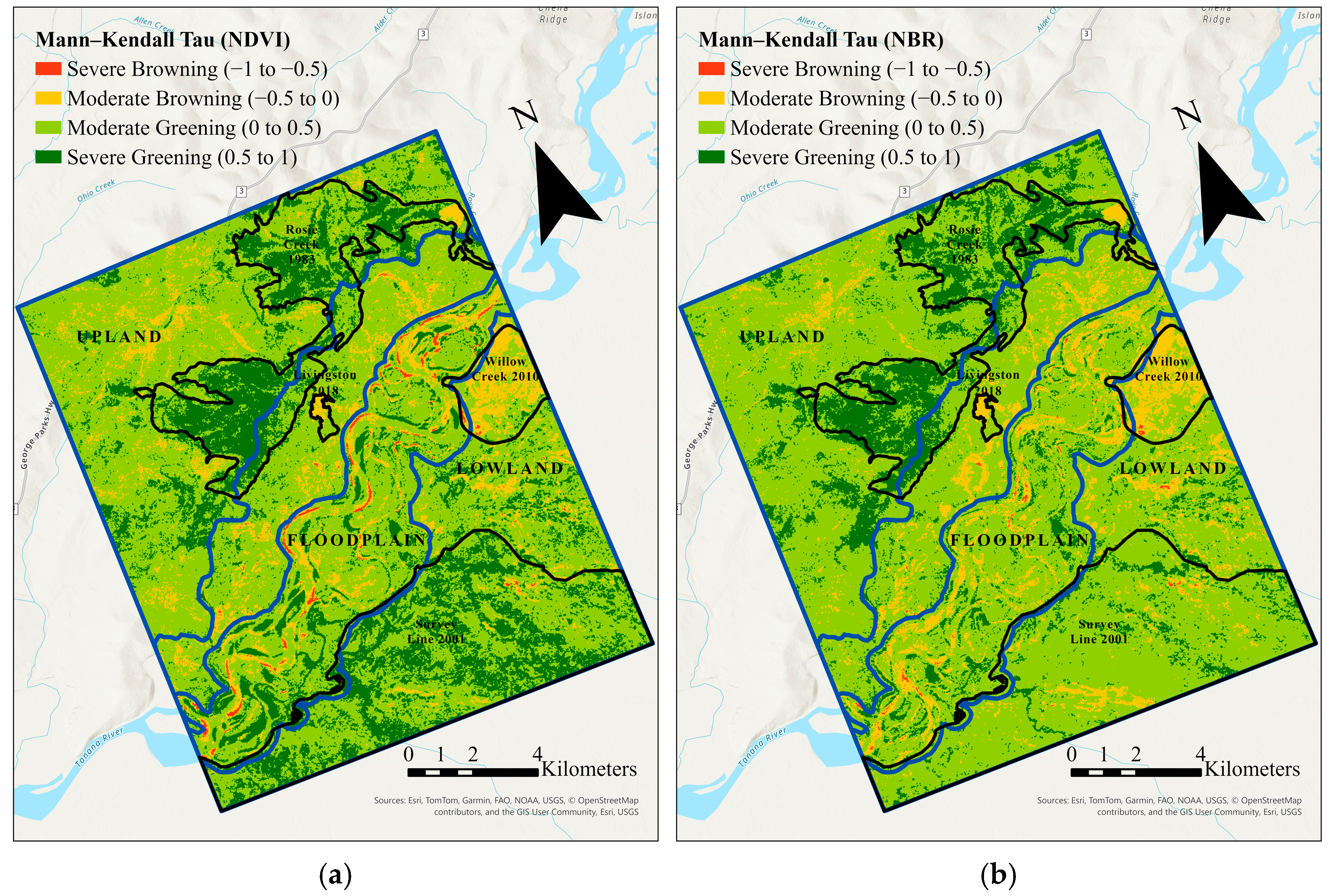
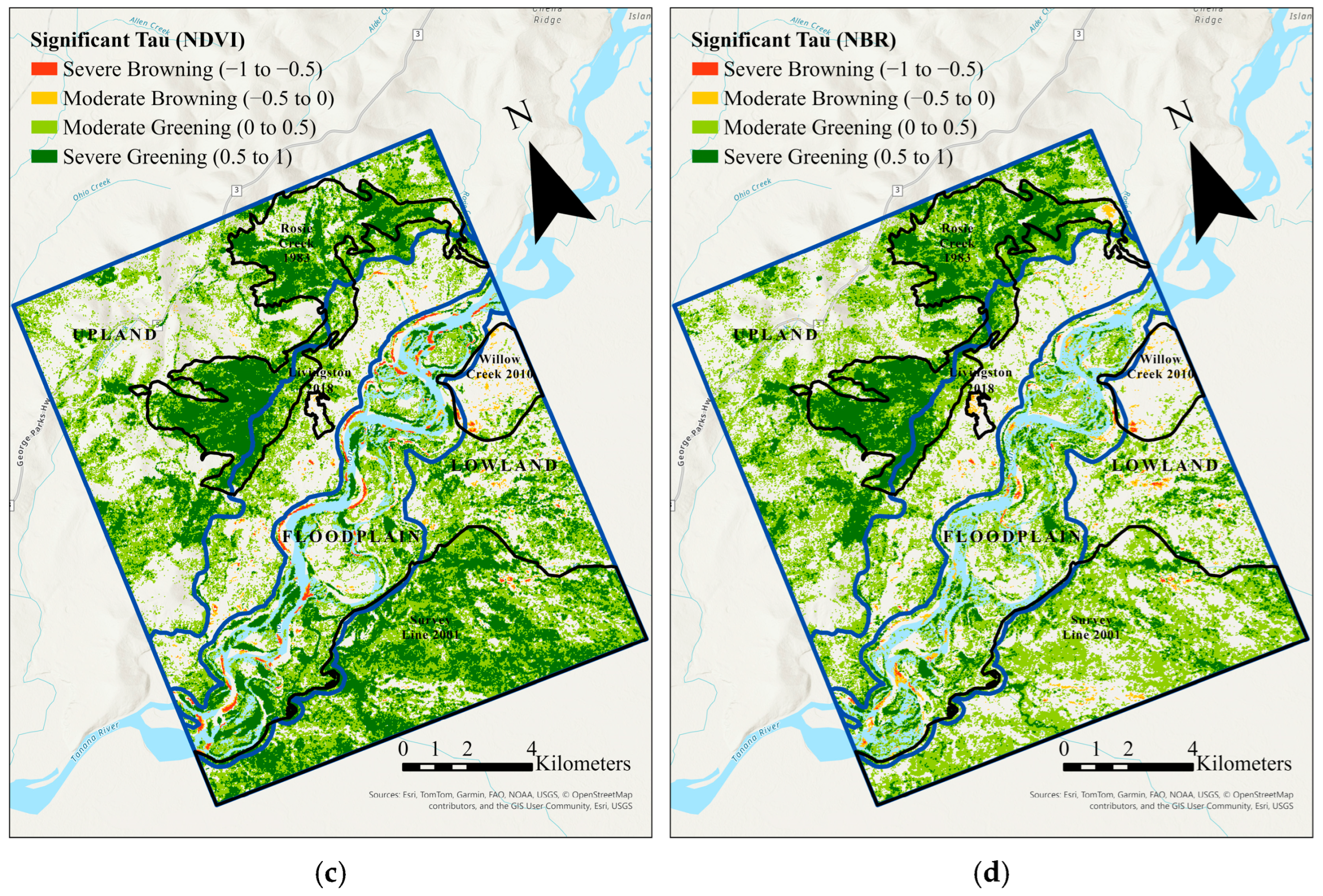
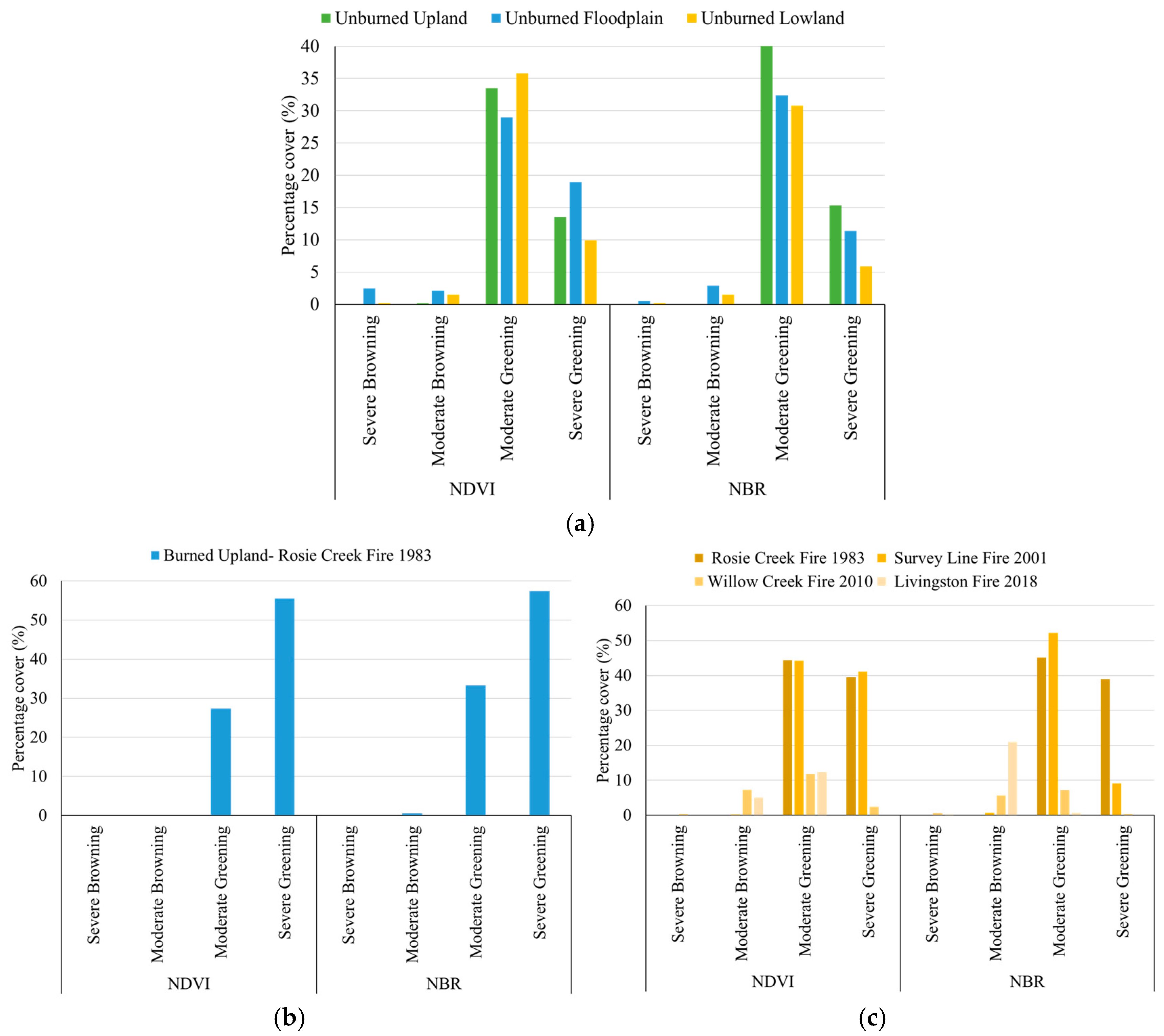
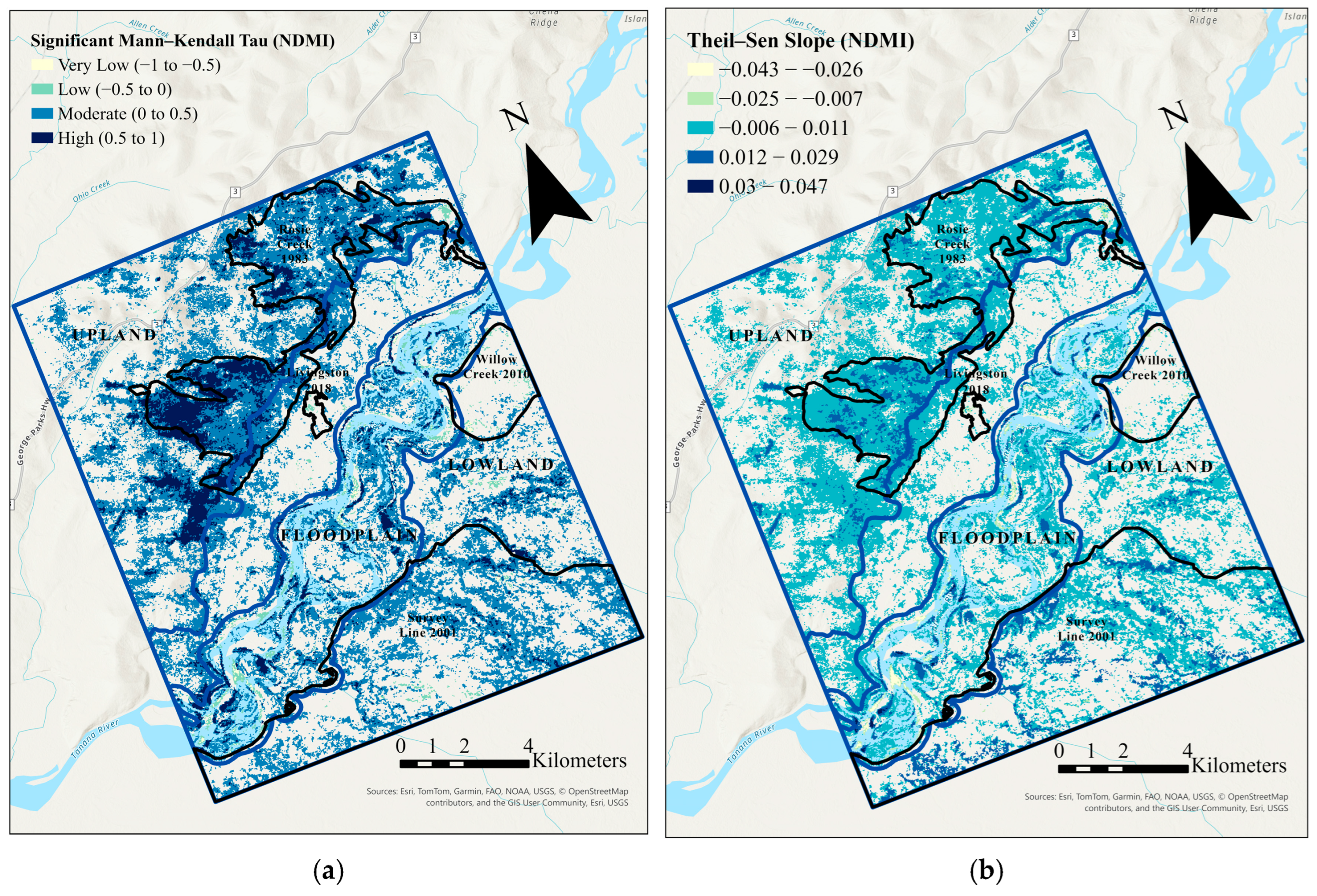
3.1. Trends in Vegetation Canopy Across the Study Area Characterized by Topography and Fire History

The trend maps (2000–2023), generated using NDVI and NBR summer maximum composites, display significant greening across all topographic units, with minor differences in the percentage cover of moderate and severe greening (Figure 3).
Both NDVI and NBR trend maps show a high percentage of greening across all unburned topographic units. The NDVI-based trend maps (Figure 4a) indicate the highest percentage of severe greening in floodplains, followed by uplands and lowlands, while the highest percentage of moderate greening is observed in lowlands, followed by uplands and floodplains. In contrast, the NBR-based trend maps show the highest percentage of severe and moderate greening in uplands, followed by floodplains and lowlands.
In burned areas, NDVI and NBR trend maps indicate substantial greening in the Rosie Creek and Survey Line burn sites. Regions affected by more recent fires, such as the 2010 Willow Creek fire and the 2018 Livingston fire, exhibit a browning trend, but only a small percentage of pixels show statistically significant change. However, NBR-based trend maps reveal a higher percentage of browning in these areas compared to NDVI trend maps. In the upland area burned by the 1983 Rosie Creek fire, both NDVI and NBR-based trend maps (Figure 4b) show similar trends, with a high percentage of severe greening. However, in the lowland area burned by the 2001 Survey Line fire, the percentage of severe greening is much higher in the NDVI trend map compared to the NBR trend map (Figure 4c).
The Theil–Sen slope maps of NDVI and NBR (Figure 5) display moderate slope values overall, indicating a gradual greening process. However, in the upland areas burned by the 1983 Rosie Creek fire, the NBR-based maps show a higher percentage of high slope values, while the NDVI-based maps display a very low percentage. In contrast, both NDVI and NBR-based maps show higher percentages of high slope values in the lowland areas burned by the 2001 Survey Line fire.

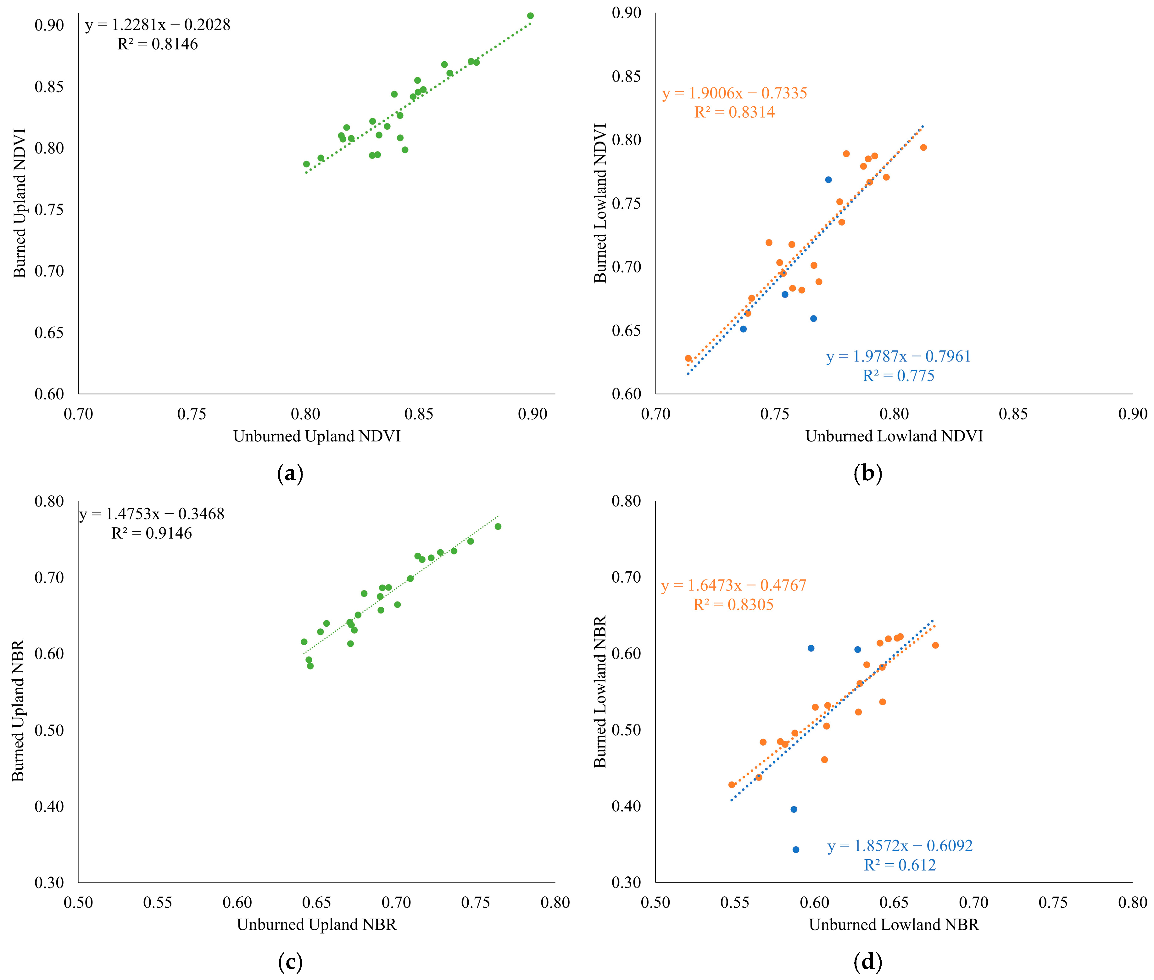
3.2. Temporal Analysis of Spectral Metrics to Assess Post-Fire Photosynthetic Recovery of Canopy

We analyzed the temporal dynamics of NDVI and NBR in burned and unburned areas of uplands and lowlands for two major fires: (1) the 1983 Rosie Creek fire in the uplands and (2) the 2001 Survey Line fire in the lowlands.
In the uplands, the mean summer maximum NDVI (Figure 6a) and NBR (Figure 6b) increased over time for both burned and unburned areas. By around 2012, NDVI and NBR values in burned areas began to converge with those in unburned areas, indicating that photosynthetic activity in the burned areas had recovered to levels similar to unburned areas, approximately 30 years after the Rosie Creek fire. The convergence in NDVI was more pronounced compared to NBR.
In the lowlands, the mean summer maximum NDVI (Figure 6c) and NBR (Figure 6d) for burned areas showed a stronger increasing trend compared to unburned areas. By 2019, NDVI values in burned and unburned areas began to converge, reaching similar levels 18 years after the 2001 Survey Line fire. Although NBR values in burned areas have also approached those in unburned areas, they have not yet fully converged.
We also examined the correlation between the burned and unburned areas in both upland and lowland using the mean summer maximum NDVI and NBR (Figure 7). The strongest correlation was observed between mean summer maximum NBR of burned and unburned upland areas, with an R-squared value of 0.91. The variance explained (R-squared) in burned and unburned lowland for both the metrics was moderate. However, after removing values from years 2001 to 2004, which includes the years immediately following the Survey Line fire, the R-squared values for both NDVI and NBR increased notably, reaching 0.83.

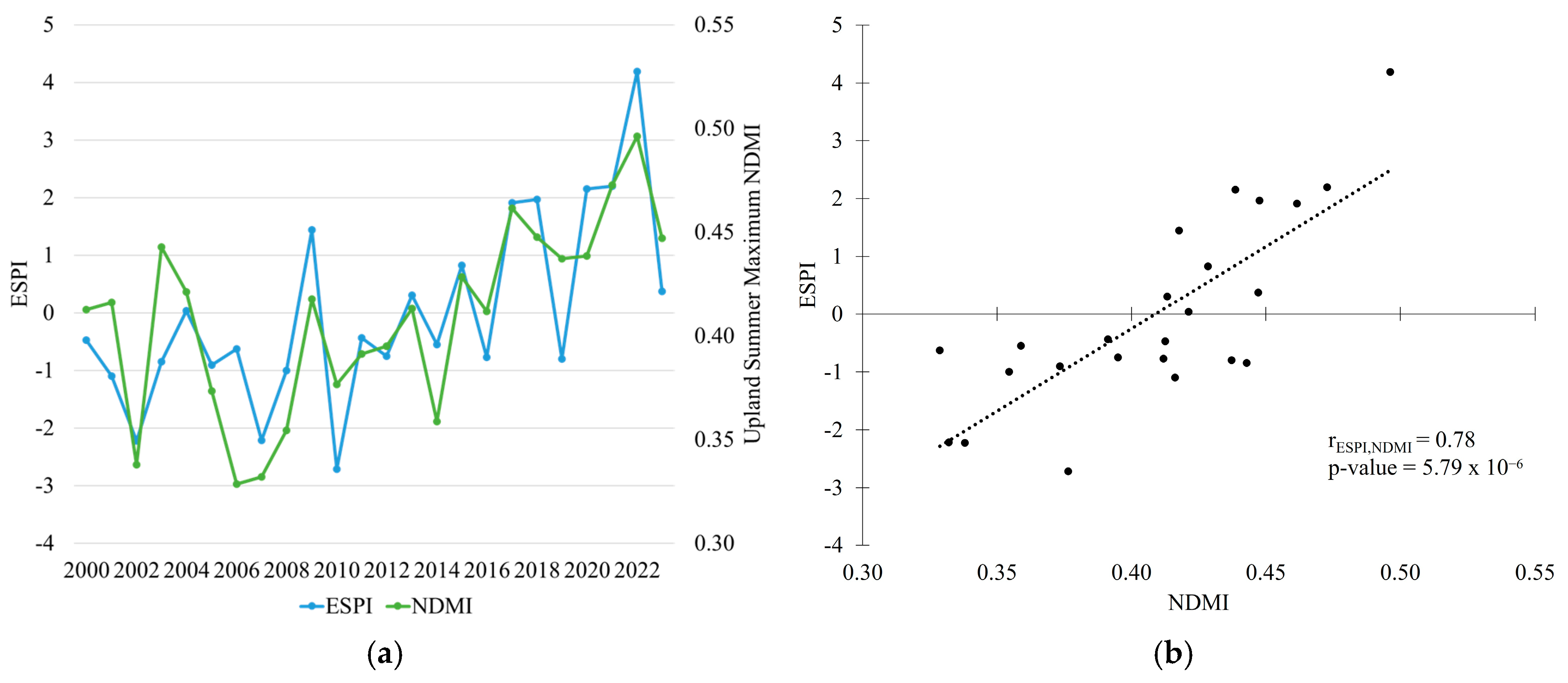
3.3. Correlation Between Spectral Metrics and Climate Variables

To better understand the impact of climate on forest canopy characteristics, we used NDVI and NDMI spectral metrics. To begin with, we calculated the Mann–Kendall trend and Theil Sen slope using annual summer maximum NDMI composites from 2000 to 2023 (Figure 8). Our findings revealed moderate to high increases in both the trend and magnitude of vegetation moisture content in uplands. Additionally, we observed a moderate increase in the trend and magnitude of moisture in lowlands. Overall, the uplands showed a higher percentage of increasing canopy moisture content over the time period of our study compared to other topographic units. We further calculated the correlation of unburned (presumably less trended than burned recovery areas) upland (Table 2) and lowland (Table 3) spectral metrics with climate variables.
The Pearson correlation coefficient (r) and p-values between the summer maximum NDVI and NDMI of the unburned upland area and various climate variables, both with and without temporal lags, are detailed in Table 2. Both indices demonstrated significant correlation with the lagged annual precipitation variables and the spring mean snow depth without any lag. As NDMI effectively indicates moisture presence in the canopy, it showed strong correlations with 1-year lagged annual total precipitation (0.73) and no-lag spring mean snow depth (0.56). This suggested that the upland vegetation canopy condition in any given year was influenced by the previous year’s precipitation and the current year’s spring mean snow depth. To further explore this relationship, we normalized the data for 1-year lag annual total precipitation and spring mean snow depth, and combined them to form the Effective Seasonal Precipitation Index (ESPI), see Equation (6). We then assessed the correlation of ESPI with NDVI and NDMI. We found that ESPI had a higher correlation with NDMI than the two individual precipitation components that compose it at r = 0.78 (Figure 9).
ESPI(year) = Normalized Annual Total Precipitation(year−1)
                + Normalized Spring Mean Snowdepth(year)
Another important correlation was observed between the unburned upland NDVI and NDMI with a 1-year lagged growing season length. There was a low and insignificant correlation between the spectral metrics and growing degree days. However, growing season length, which is calculated as continuous days with temperatures above 28 °F/−2.22 °C, is significantly correlated.
The Pearson correlation(r) and p-values between summer maximum NDVI and NDMI of the unburned lowland area and climate variables with and without lags are presented in Table 3. NDMI is only moderately but significantly correlated with 1-year lagged annual total precipitation. However, NDVI showed significant but moderate correlations with several climate indices, including lagged annual total precipitation, annual mean temperature, growing season length, and unlagged mean spring snow depth.
Across both upland and lowland sites, nSPI and the nCFI showed stronger correlations with the spectral metrics than nTFI (Table 4). In upland areas, nSPI demonstrated a moderate positive correlation with NDMI (r = 0.56, p = 0.04), while nCFI also showed a significant correlation with NDMI (r = 0.50, p = 0.01). Similarly, in lowland areas, both nSPI (r = 0.45, p = 0.02) and nCFI (r = 0.51, p = 0.01) were significantly correlated with NDMI. nCFI was also significantly correlated with NDVI in the lowlands (r = 0.42, p = 0.04), with nSPI showing a near-significant trend (r = 0.39, p = 0.06). In contrast, nTFI exhibited weak and non-significant correlations across all spectral metrics and topographic types. Since nCFI is derived from the sum of nSPI and nTFI, its observed correlations with NDVI and NDMI appear to be primarily driven by the stronger influence of nSPI, while the contribution from nTFI is minimal.

4. Discussion

4.1. Interpretation of Vegetation Canopy Trends Across the Study Area Characterized by Topography and Fire History

Greening and browning trends are influenced by factors such as the selection of time period, spatial resolution of satellite data, and size of the study area. Previous studies, which examined similar geographic areas and satellite resolutions [37,40], reported an increase in the browning trend in Interior Alaska during the period of their study. However, our findings indicate a shift towards increased greening when the analysis is extended through 2023, aligning with our hypothesis that vegetation trends may have changed due to post-fire recovery or changing precipitation patterns. The different time periods covered by these studies underscore the importance of using long-term Landsat data to accurately monitor vegetation growth and recovery.
Across all unburned topographic units, the dominant trend observed was greening. When comparing these units (Figure 4a), NDVI-based trends revealed a severe greening trend in floodplains, followed by uplands and lowlands, while a moderate greening trend was most prominent in lowlands, followed by uplands and then floodplains. The higher percentage of greening observed in floodplains may indicate intense but localized vegetation growth, possibly due to primary succession triggered by a steady supply of nutrients from the newly deposited sediments from river meandering and flooding events [65]. Greening in lowlands could be attributed to dense coverage of mosses and other ground vegetation that respond rapidly to moisture and temperature changes, potentially due to permafrost thawing [66]. Early successional plants found in these boreal environments may lead to an overestimation of NDVI, contributing to the increased greening trend.
In contrast, NBR-based trends (Figure 4a) showed the highest percentage of both severe and moderate greening in unburned uplands, followed by floodplains and then lowlands. The highest greening trend in uplands is primarily due to the presence of closed and open mixed needleleaf and hardwood forests as well as hardwood and shrub communities in well-drained soils [1,3]. The decreasing greening trend in floodplains and lowlands is likely associated with wetland vegetation types found in poorly drained soils [1].
In the upland area burned by the 1983 Rosie Creek fire, both NDVI- and NBR-based trend maps (Figure 4b) showed similar trends, with a higher percentage of severe greening. Regions affected by more recent fires, such as the 2010 Willow Creek fire and the 2018 Livingston fire, exhibited a moderate browning trend, with a small percentage of pixels showing significant change. However, NBR-based trend maps revealed a higher percentage of browning in these areas compared to NDVI trend maps. Moreover, in the lowland area burned by the 2001 Survey Line fire, the percentage of severe greening was much higher in the NDVI trend map compared to the NBR trend map (Figure 4c). This finding is consistent with previous research indicating that NDVI may overestimate vegetation recovery due to its sensitivity to herbaceous and early successional species that quickly colonize burned areas. Conversely, NBR provides a more nuanced view of recovery, capturing the slower regrowth of tree species and more accurately reflecting the long-term impacts of severe fires [55,67].
Although both NDVI and NBR trend maps indicated severe greening in the Rosie Creek fire area, the NBR-based Theil–Sen slope map (Figure 5b) showed a greater percentage of pixels with high magnitude of greening compared to the NDVI-based slope map. In the more recent Survey Line Fire area, the NDVI trend map displayed a greater percentage of severe greening, while the NBR trend map indicated only moderate greening, suggesting ongoing recovery. However, both NDVI- and NBR-based Theil–Sen slope maps (Figure 5a,b) revealed pixels with a high magnitude of change in this area, confirming that NDVI tends to overestimate severe greening, whereas NBR more accurately captures the gradual greening pattern.
Overall, the trend analysis clearly demonstrates that spectral metrics can exhibit varying responses to vegetation composition across different topographic settings.

4.2. Post-Fire Recovery of Photosynthetic Activity in Canopy

Fire has historically been a key driver of succession and vegetation dynamics in boreal ecosystems [68]. However, the changing climate is increasing the fire size and frequency and changing the evergreen forested landscapes to more persistent deciduous-dominated landscapes [18,26,69]. Due to the emergence of carbon offset markets in Alaska, forest managers are currently selling the carbon sequestration capacity of forested lands, which requires improved forest growth assessment over large remote areas.
The convergence of NDVI and NBR values in upland burned areas with unburned areas by 2012, approximately 30 years after the 1983 Rosie Creek fire (Figure 6a,b), suggests a significant recovery of photosynthetic activity and a potential shift in forest composition. This short convergence time aligns with previous studies [27,70,71,72] that document an increase in deciduous cover during post-fire succession in boreal forests. This transition can offset carbon losses and their associated deductions from marketed carbon credits caused by wildfires because deciduous-dominated stands sequester carbon more rapidly during early successional stages. In addition, deciduous stands are less flammable than coniferous forests, potentially reducing future fire severity and prolonging carbon tenure on the landscape [30].
The convergence of NDVI values in lowland areas burned during the 2001 Survey Line fire by 2019 (18 years post-fire) reflects the rapid recovery of photosynthetic activity (Figure 6c,d). This is consistent with observations that rapid growth deciduous species, such as willows, birch, and aspen, quickly regenerate in wetter, lowland environments after fire disturbances. The delayed convergence of NBR compared to NDVI supports its sensitivity to structural changes in vegetation, as NBR better captures canopy density and recovery dynamics.
Additionally, the high correlation between burned and unburned spectral metrics (Figure 7) in both upland and lowland supports the conclusion that remotely sensed spectral metrics capture the influence of similar environmental factors on vegetation greenness irrespective of its composition.

4.3. Effect of Climate on Boreal Forest Canopy

Temperature increases in the boreal region are expressed in several forms. These include a decline in the number of extremely cold days (e.g., −20 to −40 °C), and warmer summers and winters. Additionally, shifts in seasonal patterns such as earlier spring snowmelt and delayed snowfall in the fall are resulting in a longer growing season [73]. Furthermore, increased precipitation and changes in precipitation patterns [6] make it essential to understand how these climate changes affect boreal forest vegetation. To investigate these impacts on a landscape scale, we analyzed the Mann–Kendall trend and Theil–Sen Slope maps to understand canopy moisture dynamics across various topographies. We then correlated NDVI and NDMI spectral metrics with several climate variables, including annual total precipitation, spring mean snow depth (March-April), annual mean temperature, annual growing degree days, and growing season length (days above 28 °F/−2.22 °C).
Using the Mann–Kendall trend and Theil–Sen Slope analyses of summer maximum NDMI (Figure 8), we observed moderate to high increases in both the trend and magnitude of vegetation moisture content in uplands. This trend could be attributed to increased precipitation and changes in vegetation composition, as deciduous species have high moisture uptake [13]. The moderate increase in moisture trend and magnitude in lowlands, while less pronounced than in uplands, could result from topographic influences on water retention and differences in canopy composition, density, and structure.
In upland areas, both NDVI and NDMI showed significant correlations (Table 2) with lagged annual precipitation variables and current-year spring mean snow depth, with NDMI demonstrating the strongest correlation due to its sensitivity to vegetation moisture content [47]. We also found that upland vegetation condition in a given year is influenced by the previous year’s precipitation and the current year’s spring snow depth, combined into the ESPI (Figure 9). The strong correlation between ESPI and NDMI highlights ESPI’s potential for monitoring vegetation moisture dynamics at the landscape scale. Interestingly, there was only a low and insignificant correlation between upland spectral metrics and growing degree days (a measure of accumulated favorable temperatures for canopy growth). However, growing season length, defined as the continuous days with temperatures above 28 °F (−2.22 °C), during which frost-hardy vegetation typical of this region begins its physiological activity, was significantly correlated with the spectral metrics. This indicates that upland vegetation “greenness” is more responsive to climate warming influences involving extended periods of suitable warmth rather than increases in daily temperature during the growing season, at least within the temperature range that occurred during this study, with the possible exception of the record warm summer of 2004.
In the lowlands, NDMI exhibited a significant yet moderate correlation with 1-year lagged annual total precipitation. Lowlands are already moisture rich environments. This moderate correlation indicates that despite the availability of moisture, increased precipitation also impacts the vegetation in the lowlands (Table 3). NDVI, on the other hand, demonstrated significant but moderate correlations with several climate indices, including lagged annual total precipitation, annual mean temperature, growing season length, and unlagged mean spring snow depth. These results highlight the usefulness of NDVI in lowland areas, where vegetation is less dense compared to uplands, and the moisture-rich conditions make NDVI more effective for capturing climate influences.
While the Climate Favorability Index (CFI) has been widely recognized in the literature for its strong correlation with tree-ring data, our analysis reveals that satellite-derived spectral metrics—NDVI and NDMI—are more closely associated with the precipitation component (nSPI) than with the CFI as a whole. This is consistent with the positive correlation of spectral metrics with ESPI. Together, these findings suggest that within the spatial and temporal scope of this study, satellite-derived vegetation indices are particularly sensitive to interannual variability in precipitation. This highlights the critical role of moisture availability in driving vegetation greenness and moisture content in this region and underscores the potential for increased precipitation to mitigate temperature-induced stress on vegetation.

5. Conclusions

This study addresses a critical knowledge gap in understanding the complex interplay between climate change, fire history, and vegetation dynamics across different topographic settings in the boreal region of Interior Alaska using remotely sensed spectral metrics. While previous research has examined greening and browning trends, post-fire recovery, and climate influences on boreal ecosystems [37,39,40], there was a need for an updated comprehensive analysis that integrated these factors to assess their combined impact on forest canopy characteristics at a landscape scale and that also captured a recent increase in summer precipitation.
In interior boreal Alaska, a spruce forest typically requires 50 to 100 years to regain dominance following a major disturbance, depending on fire severity, site conditions, and whether active reforestation is implemented [17,74]. The observed greening trend in burned upland areas, along with photosynthetic recovery approximately 30 years post-fire, aligns well with previous studies that suggest this timeline corresponds to peak productivity during intermediate stages of boreal forest succession driven by deciduous dominance [27,70,71,72]. Our findings also address the knowledge gap regarding the role of increased precipitation during the period of recent elevated temperatures on vegetation growth as well as how topographic position impacts moisture retention, contributing to differential vegetation responses across the landscape. While increased canopy moisture content in the upland burned area is influenced by the presence of deciduous species [13], the overall greening trend in burned and unburned upland has been positively influenced by the increased precipitation of the past decade, which has offset temperature-induced drought stress. The introduction of the ESPI provides a novel approach to quantifying these interactions, offering insights into the broader ecological implications of climate on vegetation growth and recovery. Despite being moisture-rich, lowland areas also showed a moderate positive correlation between spectral metrics and precipitation variables. In these areas, NDVI captured climate influences more effectively than NDMI. Finally, the dendrochronology-based precipitation index, which is highly correlated with tree-ring width and serves as a predictor of radial tree growth, also showed strong correlations with NDMI across topographies. This highlights the critical role of moisture availability in driving vegetation greenness and moisture content in this region.
Understanding these relationships is crucial for effective forest management, carbon offset initiatives, and predicting future ecosystem responses to ongoing environmental changes. The findings emphasize the need for continuous monitoring using remote sensing data to capture the shifting vegetation patterns and their drivers in this rapidly changing boreal ecosystem.
While this research focuses on the interior boreal forests of Alaska, we believe our methodology can be applied to other boreal regions, though verifying its applicability is beyond the scope of this paper. Recognizing that greening and browning trends are influenced by factors such as the selection of time period, spatial resolution of satellite data, and study area size, this study primarily examines the roles of precipitation, temperature, and fire disturbance. Future research could expand upon these findings by exploring the influence of other environmental variables such as permafrost thaw, site fertility, and insect outbreaks on vegetation dynamics. Specifically, investigating how such additional factors interact across different topographic settings and influence post-fire successional trajectories would provide a more comprehensive understanding of boreal ecosystem dynamics and their responses to ongoing environmental change.

Author Contributions

Conceptualization, S.S., S.K.P. and G.P.J.; methodology, S.S.; software, S.S.; validation, S.S.; formal analysis, S.S.; investigation, S.S.; resources, S.K.P., G.P.J., H.G., D.R.N.B. and K.H.; data curation, S.S.; writing—original draft preparation, S.S; writing—review and editing, S.K.P., G.P.J., H.G., D.R.N.B. and K.H.; supervision, S.K.P., G.P.J., H.G., D.R.N.B. and K.H.; funding acquisition, S.K.P. All authors have read and agreed to the published version of the manuscript.

Funding

This research was funded by the USDA National Institute of Food and Agriculture, McIntire Stennis project [Accession Number: 1026801]. Glenn Juday’s effort was partially supported by the Bonanza Creek (BNZ) LTER program, which is funded by the National Science Foundation Long-Term Ecological Research program (NSF Grant DEB-2224776) and by the USDA Forest Service, Pacific Northwest Research Station (Agreement # RJVA-PNW-20-JV-11261932-018). We would also like to acknowledge the University of Alaska Fairbanks Vice Chancellor for Research for graduate funding support.

Data Availability Statement

All data that support the findings of this study are available from the corresponding author (Sumana Sahoo) upon request.

Acknowledgments

I would like to thank Christa P. Mulder, instructor of Scientific Writing, Editing, and Revising in the Biological Science course. Her feedback has been very valuable in preparing this manuscript.

Conflicts of Interest

The authors declare no conflicts of interest.

References

  1. Viereck, L.A.; Dyrness, C.T.; Batten, A.R.; Wenzlick, K.J. The Alaska Vegetation Classification; U.S. Department of Agriculture, Forest Service, Pacific Northwest Research Station: Portland, OR, USA, 1992; p. PNW-GTR-286.
  2. Nowacki, G.J.; Spencer, P.; Fleming, M.; Brock, T.; Jorgenson, T. Unified Ecoregions of Alaska: 2001; Open-File Report; US Geological Survey: Reston, VA, USA, 2003.
  3. Chapin, F.S.; Oswood, M.W.; Van Cleve, K.; Viereck, L.A.; Verbyla, D.L. Alaska’s Changing Boreal Forest; Oxford University Press: Oxford, UK, 2006; ISBN 978-0-19-756192-8. [Google Scholar]
  4. Douglas, T.A.; Jones, M.C.; Hiemstra, C.A.; Arnold, J.R. Sources and Sinks of Carbon in Boreal Ecosystems of Interior Alaska: A Review. Elem. Sci. Anthr. 2014, 2, 000032. [Google Scholar] [CrossRef]
  5. Thoman, R.; Walsh, J.E. Alaska’s Changing Environment, 1st ed.; International Arctic Research Center, University of Alaska Fairbanks: Fairbanks, AK, USA, 2019. [Google Scholar]
  6. Thoman, R.; McFarland, H.R. Alaska’s Changing Environment, 2nd ed.; Alaska Center for Climate Assessment and Policy, International Arctic Research Center, University of Alaska Fairbanks: Fairbanks, AK, USA, 2024; Available online: https://uaf-iarc.org/communicating-change/ (accessed on 30 December 2024).
  7. Buma, B.; Hayes, K.; Weiss, S.; Lucash, M. Short-Interval Fires Increasing in the Alaskan Boreal Forest as Fire Self-Regulation Decays across Forest Types. Sci. Rep. 2022, 12, 4901. [Google Scholar] [CrossRef]
  8. Chapin, F.S.; McGuire, A.D.; Ruess, R.W.; Hollingsworth, T.N.; Mack, M.C.; Johnstone, J.F.; Kasischke, E.S.; Euskirchen, E.S.; Jones, J.B.; Jorgenson, M.T.; et al. Resilience of Alaska’s Boreal Forest to Climatic change; This Article Is One of a Selection of Papers from the Dynamics of Change in Alaska’s Boreal Forests: Resilience and Vulnerability in Response to Climate Warming. Can. J. For. Res. 2010, 40, 1360–1370. [Google Scholar] [CrossRef]
  9. Euskirchen, E.S.; McGuire, A.D.; Chapin, F.S.; Rupp, T.S. The Changing Effects of Alaska’s Boreal Forests on the Climate system; This Article Is One of a Selection of Papers from the Dynamics of Change in Alaska’s Boreal Forests: Resilience and Vulnerability in Response to Climate Warming. Can. J. For. Res. 2010, 40, 1336–1346. [Google Scholar] [CrossRef]
  10. Wolken, J.M.; Hollingsworth, T.N.; Rupp, T.S.; Chapin, F.S., III; Trainor, S.F.; Barrett, T.M.; Sullivan, P.F.; McGuire, A.D.; Euskirchen, E.S.; Hennon, P.E.; et al. Evidence and Implications of Recent and Projected Climate Change in Alaska’s Forest Ecosystems. Ecosphere 2011, 2, art124. [Google Scholar] [CrossRef]
  11. Johnstone, J.F.; Chapin, F.S.I.; Hollingsworth, T.N.; Mack, M.C.; Romanovsky, V.; Turetsky, M. Fire, Climate Change, and Forest Resilience in Interior Alaska. Can. J. For. Res. 2010, 40, 1302–1312. [Google Scholar] [CrossRef]
  12. Nicklen, E.F.; Roland, C.A.; Ruess, R.W.; Schmidt, J.H.; Lloyd, A.H. Local Site Conditions Drive Climate–Growth Responses of Picea Mariana and Picea Glauca in Interior Alaska. Ecosphere 2016, 7, e01507. [Google Scholar] [CrossRef]
  13. Young-Robertson, J.M.; Bolton, W.R.; Bhatt, U.S.; Cristóbal, J.; Thoman, R. Deciduous Trees Are a Large and Overlooked Sink for Snowmelt Water in the Boreal Forest. Sci. Rep. 2016, 6, 29504. [Google Scholar] [CrossRef] [PubMed]
  14. Roland, C.A.; Schmidt, J.H.; Winder, S.G.; Stehn, S.E.; Nicklen, E.F. Regional Variation in Interior Alaskan Boreal Forests Is Driven by Fire Disturbance, Topography, and Climate. Ecol. Monogr. 2019, 89, e01369. [Google Scholar] [CrossRef]
  15. Jin, X.-Y.; Jin, H.-J.; Iwahana, G.; Marchenko, S.S.; Luo, D.-L.; Li, X.-Y.; Liang, S.-H. Impacts of Climate-Induced Permafrost Degradation on Vegetation: A Review. Adv. Clim. Change Res. 2021, 12, 29–47. [Google Scholar] [CrossRef]
  16. Douglas, T.A.; Hiemstra, C.A.; Anderson, J.E.; Barbato, R.A.; Bjella, K.L.; Deeb, E.J.; Gelvin, A.B.; Nelsen, P.E.; Newman, S.D.; Saari, S.P.; et al. Recent Degradation of Interior Alaska Permafrost Mapped with Ground Surveys, Geophysics, Deep Drilling, and Repeat Airborne Lidar. Cryosphere 2021, 15, 3555–3575. [Google Scholar] [CrossRef]
  17. Johnstone, J.F.; Chapin, F.S. Effects of Soil Burn Severity on Post-Fire Tree Recruitment in Boreal Forest. Ecosystems 2006, 9, 14–31. [Google Scholar] [CrossRef]
  18. Johnstone, J.F.; Rupp, T.S.; Olson, M.; Verbyla, D. Modeling Impacts of Fire Severity on Successional Trajectories and Future Fire Behavior in Alaskan Boreal Forests. Landsc. Ecol. 2011, 26, 487–500. [Google Scholar] [CrossRef]
  19. Johnstone, J.F.; Hollingsworth, T.N.; Chapin, F.S., III; Mack, M.C. Changes in Fire Regime Break the Legacy Lock on Successional Trajectories in Alaskan Boreal Forest. Glob. Change Biol. 2010, 16, 1281–1295. [Google Scholar] [CrossRef]
  20. Massey, R.; Rogers, B.M.; Berner, L.T.; Cooperdock, S.; Mack, M.C.; Walker, X.J.; Goetz, S.J. Forest Composition Change and Biophysical Climate Feedbacks across Boreal North America. Nat. Clim. Change 2023, 13, 1368–1375. [Google Scholar] [CrossRef]
  21. Kasischke, E.S.; Williams, D.; Barry, D. Analysis of the Patterns of Large Fires in the Boreal Forest Region of Alaska. Int. J. Wildland Fire 2002, 11, 131. [Google Scholar] [CrossRef]
  22. Turetsky, M.R.; Kane, E.S.; Harden, J.W.; Ottmar, R.D.; Manies, K.L.; Hoy, E.; Kasischke, E.S. Recent Acceleration of Biomass Burning and Carbon Losses in Alaskan Forests and Peatlands. Nat. Geosci. 2011, 4, 27–31. [Google Scholar] [CrossRef]
  23. Brown, E.K.; Wang, J.; Feng, Y. US Wildfire Potential: A Historical View and Future Projection Using High-Resolution Climate Data. Environ. Res. Lett. 2021, 16, 034060. [Google Scholar] [CrossRef]
  24. Weiss, S.A.; Marshall, A.M.; Hayes, K.R.; Nicolsky, D.J.; Buma, B.; Lucash, M.S. Future Transitions from a Conifer to a Deciduous-Dominated Landscape Are Accelerated by Greater Wildfire Activity and Climate Change in Interior Alaska. Landsc. Ecol. 2023, 38, 2569–2589. [Google Scholar] [CrossRef]
  25. Goetz, S.J.; Bunn, A.G.; Fiske, G.J.; Houghton, R.A. Satellite-Observed Photosynthetic Trends across Boreal North America Associated with Climate and Fire Disturbance. Proc. Natl. Acad. Sci. USA 2005, 102, 13521–13525. [Google Scholar] [CrossRef]
  26. Shenoy, A.; Johnstone, J.F.; Kasischke, E.S.; Kielland, K. Persistent Effects of Fire Severity on Early Successional Forests in Interior Alaska. For. Ecol. Manag. 2011, 261, 381–390. [Google Scholar] [CrossRef]
  27. Beck, P.S.A.; Goetz, S.J. Satellite Observations of High Northern Latitude Vegetation Productivity Changes between 1982 and 2008: Ecological Variability and Regional Differences. Environ. Res. Lett. 2011, 6, 045501. [Google Scholar] [CrossRef]
  28. Mekonnen, Z.A.; Riley, W.J.; Randerson, J.T.; Grant, R.F.; Rogers, B.M. Expansion of High-Latitude Deciduous Forests Driven by Interactions between Climate Warming and Fire. Nat. Plants 2019, 5, 952–958. [Google Scholar] [CrossRef]
  29. Bernier, P.Y.; Gauthier, S.; Jean, P.-O.; Manka, F.; Boulanger, Y.; Beaudoin, A.; Guindon, L. Mapping Local Effects of Forest Properties on Fire Risk across Canada. Forests 2016, 7, 157. [Google Scholar] [CrossRef]
  30. Mack, M.C.; Walker, X.J.; Johnstone, J.F.; Alexander, H.D.; Melvin, A.M.; Jean, M.; Miller, S.N. Carbon Loss from Boreal Forest Wildfires Offset by Increased Dominance of Deciduous Trees. Science 2021, 372, 280–283. [Google Scholar] [CrossRef] [PubMed]
  31. Barber, V.A.; Juday, G.P.; Finney, B.P. Reduced Growth of Alaskan White Spruce in the Twentieth Century from Temperature-Induced Drought Stress. Nature 2000, 405, 668–673. [Google Scholar] [CrossRef]
  32. Lloyd, A.H.; Bunn, A.G. Responses of the Circumpolar Boreal Forest to 20th Century Climate Variability. Environ. Res. Lett. 2007, 2, 045013. [Google Scholar] [CrossRef]
  33. Juday, G.P.; Alix, C. Consistent Negative Temperature Sensitivity and Positive Influence of Precipitation on Growth of Floodplain Picea Glauca in Interior Alaska. Can. J. For. Res. 2012, 42, 561–573. [Google Scholar] [CrossRef]
  34. Walker, X.; Johnstone, J.F. Widespread Negative Correlations between Black Spruce Growth and Temperature across Topographic Moisture Gradients in the Boreal Forest. Environ. Res. Lett. 2014, 9, 064016. [Google Scholar] [CrossRef]
  35. Campbell, J.L.; Driscoll, C.T.; Jones, J.A.; Boose, E.R.; Dugan, H.A.; Groffman, P.M.; Jackson, C.R.; Jones, J.B.; Juday, G.P.; Lottig, N.R.; et al. Forest and Freshwater Ecosystem Responses to Climate Change and Variability at US LTER Sites. BioScience 2022, 72, 851–870. [Google Scholar] [CrossRef]
  36. Verbyla, D. The Greening and Browning of Alaska Based on 1982–2003 Satellite Data. Glob. Ecol. Biogeogr. 2008, 17, 547–555. [Google Scholar] [CrossRef]
  37. Parent, M.B.; Verbyla, D. The Browning of Alaska’s Boreal Forest. Remote Sens. 2010, 2, 2729–2747. [Google Scholar] [CrossRef]
  38. Verbyla, D. Browning Boreal Forests of Western North America. Environ. Res. Lett. 2011, 6, 041003. [Google Scholar] [CrossRef]
  39. Verbyla, D. Remote Sensing of Interannual Boreal Forest NDVI in Relation to Climatic Conditions in Interior Alaska. Environ. Res. Lett. 2015, 10, 125016. [Google Scholar] [CrossRef]
  40. Baird, R.A.; Verbyla, D.; Hollingsworth, T.N. Browning of the Landscape of Interior Alaska Based on 1986–2009 Landsat Sensor NDVI. Can. J. For. Res. 2012, 42, 1371–1382. [Google Scholar] [CrossRef]
  41. Berner, L.T.; Goetz, S.J. Satellite Observations Document Trends Consistent with a Boreal Forest Biome Shift. Glob. Change Biol. 2022, 28, 3275–3292. [Google Scholar] [CrossRef] [PubMed]
  42. Wulder, M.A.; White, J.C.; Loveland, T.R.; Woodcock, C.E.; Belward, A.S.; Cohen, W.B.; Fosnight, E.A.; Shaw, J.; Masek, J.G.; Roy, D.P. The Global Landsat Archive: Status, Consolidation, and Direction. Remote Sens. Environ. 2016, 185, 271–283. [Google Scholar] [CrossRef]
  43. Huete, A.R.; Liu, H.; van Leeuwen, W.J.D. The Use of Vegetation Indices in Forested Regions: Issues of Linearity and Saturation. In Proceedings of the IGARSS’97. 1997 IEEE International Geoscience and Remote Sensing Symposium Proceedings. Remote Sensing—A Scientific Vision for Sustainable Development, Singapore, 3–8 August 1997; Volume 4, pp. 1966–1968. [Google Scholar]
  44. Mutanga, O.; Skidmore, A.K. Narrow Band Vegetation Indices Overcome the Saturation Problem in Biomass Estimation. Int. J. Remote Sens. 2004, 25, 3999–4014. [Google Scholar] [CrossRef]
  45. Epting, J.; Verbyla, D.; Sorbel, B. Evaluation of Remotely Sensed Indices for Assessing Burn Severity in Interior Alaska Using Landsat TM and ETM+. Remote Sens. Environ. 2005, 96, 328–339. [Google Scholar] [CrossRef]
  46. Pickell, P.D.; Coops, N.C.; Gergel, S.E.; Andison, D.W.; Marshall, P.L. Evolution of Canada’s Boreal Forest Spatial Patterns as Seen from Space. PLoS ONE 2016, 11, e0157736. [Google Scholar] [CrossRef]
  47. Hunt, E.R.; Wang, L.; Qu, J.J.; Hao, X. Remote Sensing of Fuel Moisture Content from the Ratios of Canopy Water Indices with a Foliar Dry Matter Index. In Proceedings of the Remote Sensing and Modeling of Ecosystems for Sustainability IX, SPIE, San Diego, CA, USA, 24 October 2012; Volume 8513, pp. 9–16. [Google Scholar]
  48. Juday, G.P. The Rosie Creek Fire. Agroborealis 1985, 17, 11–20. [Google Scholar]
  49. Wulder, M.A.; Roy, D.P.; Radeloff, V.C.; Loveland, T.R.; Anderson, M.C.; Johnson, D.M.; Healey, S.; Zhu, Z.; Scambos, T.A.; Pahlevan, N.; et al. Fifty Years of Landsat Science and Impacts. Remote Sens. Environ. 2022, 280, 113195. [Google Scholar] [CrossRef]
  50. Zhu, Z.; Woodcock, C.E. Object-Based Cloud and Cloud Shadow Detection in Landsat Imagery. Remote Sens. Environ. 2012, 118, 83–94. [Google Scholar] [CrossRef]
  51. Zhu, Z.; Wang, S.; Woodcock, C.E. Improvement and Expansion of the Fmask Algorithm: Cloud, Cloud Shadow, and Snow Detection for Landsats 4–7, 8, and Sentinel 2 Images. Remote Sens. Environ. 2015, 159, 269–277. [Google Scholar] [CrossRef]
  52. Foga, S.; Scaramuzza, P.L.; Guo, S.; Zhu, Z.; Dilley, R.D.; Beckmann, T.; Schmidt, G.L.; Dwyer, J.L.; Joseph Hughes, M.; Laue, B. Cloud Detection Algorithm Comparison and Validation for Operational Landsat Data Products. Remote Sens. Environ. 2017, 194, 379–390. [Google Scholar] [CrossRef]
  53. Wu, Q. Geemap: A Python Package for Interactive Mapping with Google Earth Engine. J. Open Source Softw. 2020, 5, 2305. [Google Scholar] [CrossRef]
  54. Tucker, C.J.; Vanpraet, C.L.; Sharman, M.J.; Van Ittersum, G. Satellite Remote Sensing of Total Herbaceous Biomass Production in the Senegalese Sahel: 1980–1984. Remote Sens. Environ. 1985, 17, 233–249. [Google Scholar] [CrossRef]
  55. Roy, D.P.; Boschetti, L.; Trigg, S.N. Remote Sensing of Fire Severity: Assessing the Performance of the Normalized Burn Ratio. IEEE Geosci. Remote Sens. Lett. 2006, 3, 112–116. [Google Scholar] [CrossRef]
  56. Mann, H.B. Nonparametric Tests Against Trend. Econometrica 1945, 13, 245–259. [Google Scholar] [CrossRef]
  57. Kendall, M.G. Rank Correlation Methods; Griffin: Oxford, UK, 1948. [Google Scholar]
  58. Sen, P.K. Estimates of the Regression Coefficient Based on Kendall’s Tau. J. Am. Stat. Assoc. 1968, 63, 1379–1389. [Google Scholar] [CrossRef]
  59. Theil, H. A Rank-Invariant Method of Linear and Polynomial Regression Analysis. In Henri Theil’s Contributions to Economics and Econometrics; Raj, B., Koerts, J., Eds.; Advanced Studies in Theoretical and Applied Econometrics; Springer: Dordrecht, The Netherlands, 1992; Volume 23, pp. 345–381. ISBN 978-94-010-5124-8. [Google Scholar]
  60. Hussain, M.; Mahmud, I. pyMannKendall: A Python Package for Non Parametric Mann Kendall Family of Trend Tests. J. Open Source Softw. 2019, 4, 1556. [Google Scholar] [CrossRef]
  61. Hamed, K.H.; Ramachandra Rao, A. A Modified Mann-Kendall Trend Test for Autocorrelated Data. J. Hydrol. 1998, 204, 182–196. [Google Scholar] [CrossRef]
  62. Gamon, J.; Field, C.; Goulden, M.; Griffin, K.; Hartley, A.; Joel, G.; Penuelas, J.; Valentini, R. Relationships Between NDVI, Canopy Structure, and Photosynthesis in Three Californian Vegetation Types. Ecol. Appl. 1995, 5, 28–41. [Google Scholar] [CrossRef]
  63. Ensminger, I.; Schmidt, L.; Lloyd, J. Soil Temperature and Intermittent Frost Modulate the Rate of Recovery of Photosynthesis in Scots Pine under Simulated Spring Conditions. New Phytol. 2008, 177, 428–442. [Google Scholar] [CrossRef]
  64. Grossnicke, S.C. Ecophysiology of Northern Spruce Species: The Performance of Planted Seedlings, 1st ed.; NRC Research Press: Ottawa, ON, Canada, 2000; ISBN 978-0-660-17959-9. [Google Scholar]
  65. Stuart, F.; Viereck, L.A.; Adams, P.C.; Cleve, K.; Fastie, C.; Ott, R.; Mann, D.; Johnstone, J. Successional Processes in the Alaskan Boreal Forest, Chapin III; Oxford University Press Inc.: New York, NY, USA, 2006; ISBN 978-0-19-515431-3. [Google Scholar]
  66. Jorgenson, M.T.; Racine, C.H.; Walters, J.C.; Osterkamp, T.E. Permafrost Degradation and Ecological Changes Associated with a Warming Climate in Central Alaska. Clim. Change 2001, 48, 551–579. [Google Scholar] [CrossRef]
  67. Morresi, D.; Vitali, A.; Urbinati, C.; Garbarino, M. Forest Spectral Recovery and Regeneration Dynamics in Stand-Replacing Wildfires of Central Apennines Derived from Landsat Time Series. Remote Sens. 2019, 11, 308. [Google Scholar] [CrossRef]
  68. Kasischke, E.S.; Verbyla, D.L. Fire Trends in the Alaskan Boreal Forest. In Alaska’s Changing Boreal Forest; Chapin, F.S., Oswood, M.W., Van Cleve, K., Viereck, L.A., Verbyla, D.L., Eds.; Oxford University Press Inc.: Oxford, New York, 2006; pp. 285–301. ISBN 978-0-19-515431-3. [Google Scholar]
  69. Euskirchen, E.S.; McGuire, A.D.; Chapin, F.S., III; Yi, S.; Thompson, C.C. Changes in Vegetation in Northern Alaska under Scenarios of Climate Change, 2003–2100: Implications for Climate Feedbacks. Ecol. Appl. 2009, 19, 1022–1043. [Google Scholar] [CrossRef]
  70. Johnstone, J.F.; Chapin, F.S., III; Foote, J.; Kemmett, S.; Price, K.; Viereck, L. Decadal Observations of Tree Regeneration Following Fire in Boreal Forests. Can. J. For. Res. 2004, 34, 267–273. [Google Scholar] [CrossRef]
  71. Beck, P.S.A.; Goetz, S.J.; Mack, M.C.; Alexander, H.D.; Jin, Y.; Randerson, J.T.; Loranty, M.M. The Impacts and Implications of an Intensifying Fire Regime on Alaskan Boreal Forest Composition and Albedo. Glob. Change Biol. 2011, 17, 2853–2866. [Google Scholar] [CrossRef]
  72. Kim, J.E.; Wang, J.A.; Li, Y.; Czimczik, C.I.; Randerson, J.T. Wildfire-Induced Increases in Photosynthesis in Boreal Forest Ecosystems of North America. Glob. Change Biol. 2024, 30, e17151. [Google Scholar] [CrossRef]
  73. The Oxford Companion to Global Change. Goudie, E.A.; Cuff, D. (Eds.) Oxford Companions; Oxford University Press: Oxford, UK; New York, NY, USA, 2008; ISBN 978-0-19-532488-4. [Google Scholar]
  74. Hollingsworth, T.N.; Johnstone, J.F.; Bernhardt, E.L.; Chapin, F.S., III. Fire Severity Filters Regeneration Traits to Shape Community Assembly in Alaska’s Boreal Forest. PLoS ONE 2013, 8, e56033. [Google Scholar] [CrossRef] [PubMed]
Figure 1. The study area is stratified into three topographic units: upland (green), lowland (yellow), and floodplain (blue) and further stratified into burned (hatched) and unburned areas (unhatched) using historical fire polygons.
Forests 16 00777 g001
Figure 2. A flowchart of the data processing workflow and analysis implemented in this study.
Forests 16 00777 g002
Figure 3. Mann–Kendall trend maps (2000–2023) derived using annual summer maximum composites of (a) NDVI and (b) NBR, along with corresponding significant trend maps (p < 0.05) (c) NDVI and (d) NBR. Historic fire perimeters are marked by solid black lines. Severe greening trends appear in NDVI and NBR maps within 1984 Rosie Creek Fire polygons, with variations in the 2001 Survey Line Fire polygon.
Forests 16 00777 g003aForests 16 00777 g003b
Figure 4. Comparison of percentage cover of NDVI and NBR based on significant trends across (a) unburned areas in topographic units, (b) burned areas in upland, and (c) burned areas in lowland.
Forests 16 00777 g004
Figure 5. Theil–Sen slope maps derived using (a) NDVI, (b) NBR.
Forests 16 00777 g005
Figure 6. Comparison of (a) burned and unburned upland NDVI, (b) burned and unburned upland NBR, (c) burned and unburned lowland NDVI, (d) burned and unburned lowland NBR from 2000 to 2023.
Forests 16 00777 g006
Figure 7. Correlation of (a) burned upland NDVI vs. unburned upland NDVI, (b) burned lowland NDVI vs. unburned lowland NDVI, (c) burned upland NBR vs. unburned upland NBR, (d) burned lowland NBR vs. unburned lowland NBR. (Orange trendline and equations represent lowland trend excluding years 2001–2004 in blue).
Forests 16 00777 g007
Figure 8. (a) Significant Mann–Kendall trend map (p < 0.05) and (b) Theil–Sen slope map using annual summer maximum NDMI composites from 2000 to 2023. There is moderate to high increase in the trend and magnitude of vegetation moisture in uplands, while lowlands exhibit a moderate increase.
Forests 16 00777 g008
Figure 9. (a) Temporal congruence between ESPI and NDMI and (b) linear trend and correlation of ESPI vs. NDMI.
Forests 16 00777 g009
Table 1. The literature emphasizes the use of satellite observations to study canopy trends in Alaska.
StudyStudy PeriodSatellite DataSpatial ResolutionTemporal ResolutionExtentStudy Area
[36]1982–2003GIMMS-NDVI64 km 15-day compositeRegionalArctic and sub-arctic Alaska
[37]1980–2009Landsat-NDVI30 m16-day revisitScene-basedInterior Boreal
1981–2008GIMMS-NDVI64 km 15-day compositeRegional
2000–2009MODIS-NDVI1 km16-day compositeRegional
[39]2000–2014MODIS-NDVI250 m8-day compositeRegionalInterior Boreal
[27]1982–2008GIMMS-NDVI
MODIS-NDVI
0.07°
1 km
15-day composite
Monthly
ContinentalNorth America and Eurasia
[40]1986–2009Landsat NDVI30 m16-day revisitScene-basedBonanza Creek Experimental Forest
[41]1985–2019
2000–2019
(includes Alaska)
Landsat based greenness indices30 m16-day revisitContinentalCircumpolar boreal region
Table 2. Pearson correlation (r) and p-values between mean summer maximum of NDVI and NDMI for unburned upland with various climate variables. Significant correlations (α = 0.05) have been bolded.
Climate VariablesNDVINDMI
rp-Valuerp-Value
Annual Total Precipitation0.190.370.180.41
Annual Total Precipitation Lag 10.470.020.730.00
Annual Total Precipitation Lag 20.610.000.540.01
Annual Total Precipitation Lag 30.590.000.450.03
Spring Mean Snow depth0.680.000.560.00
Spring Mean Snow depth Lag 10.300.160.200.35
Spring Mean Snow depth Lag 20.100.640.050.81
Spring Mean Snow depth Lag 30.010.960.200.34
Annual Mean Temperature0.220.300.270.20
Annual Mean Temperature Lag 10.070.730.260.21
Annual Mean Temperature Lag 20.340.100.360.09
Annual Mean Temperature Lag 30.520.010.420.04
Annual Growing Degree Days0.320.130.280.19
Annual Growing Degree Days Lag 10.250.24−0.010.96
Annual Growing Degree Days Lag 20.190.380.210.32
Annual Growing Degree Days Lag 30.300.15−0.070.76
Growing Season Length0.440.030.200.34
Growing Season Length Lag10.570.000.470.02
Growing Season Length Lag20.460.020.520.01
Growing Season Length Lag30.670.000.520.01
Table 3. Pearson correlation (r) and p-value (α = 0.05) between mean summer maximum of NDVI and NDMI for unburned lowland with various climate variables. Significant correlations (α = 0.05) have been bolded.
Climate VariablesNDVINDMI
rp-Valuerp-Value
Annual Total Precipitation0.260.22−0.030.89
Annual Total Precipitation Lag 10.550.010.470.02
Annual Total Precipitation Lag 20.590.000.310.14
Annual Total Precipitation Lag 30.450.030.220.29
Spring Mean Snow depth0.640.000.290.17
Spring Mean Snow depth Lag 10.220.300.190.37
Spring Mean Snow depth Lag 20.110.610.030.88
Spring Mean Snow depth Lag 30.100.65−0.030.88
Annual Mean Temperature0.260.230.210.33
Annual Mean Temperature Lag 10.120.570.240.26
Annual Mean Temperature Lag 20.510.01−0.040.85
Annual Mean Temperature Lag 30.550.010.260.22
Annual Growing Degree Days0.260.230.100.66
Annual Growing Degree Days Lag 10.070.74−0.330.12
Annual Growing Degree Days Lag 20.220.300.100.65
Annual Growing Degree Days Lag 30.270.20−0.170.44
Growing Season Length0.390.060.170.43
Growing Season Length Lag10.330.11−0.030.89
Growing Season Length Lag20.470.020.240.26
Growing Season Length Lag30.520.010.310.14
Table 4. Pearson correlation (r) and p-value (α = 0.05) between dendrochronology-based climate indices (nSPI, nTFI, nCFI) and mean summer maximum of NDVI and NDMI for unburned upland and lowland. Significant correlations (α = 0.05) have been bolded.
Dendrochronology-Based IndicesUplandLowland
NDVINDMINDVINDMI
rp-Valuerp-Valuerp-Valuerp-Value
Normalized Supplemental Precipitation Index (nSPI)0.370.070.560.040.390.060.450.02
Normalized Temperature Favorability Index (nTFI)−0.120.59−0.060.760.080.710.030.88
Normalized Climate Favorability Index (nCFI)0.270.210.500.010.420.040.510.01
Disclaimer/Publisher’s Note: The statements, opinions and data contained in all publications are solely those of the individual author(s) and contributor(s) and not of MDPI and/or the editor(s). MDPI and/or the editor(s) disclaim responsibility for any injury to people or property resulting from any ideas, methods, instructions or products referred to in the content.

