Article

Characterization of Shrub Fuel Structure and Spatial Distribution Using Multispectral and 3D Multitemporal UAV Data

by
Ramón Alberto Díaz-Varela
1,*,
Cecilia Alonso-Rego
2,
Stéfano Arellano-Pérez
3,
Carlos Iván Briones-Herrera
4,
Juan Gabriel Álvarez-González
5 and
Ana Daría Ruiz-González
5
1
GI Biodiversidad y Botánica Aplicada (GI BIOAPLIC 1809), Departamento de Botánica, Escuela Politécnica Superior de Ingeniería, R/Benigno Ledo s/n, Universidad de Santiago de Compostela, Campus Terra, 27002 Lugo, Spain
2
Departamento de Ingeniería y Ciencias Agrarias, Escuela de Ingeniería Agraria y Forestal, Avda. de Astorga 15, Universidad de León, 24401 León, Spain
3
AGRESTA Sociedad Cooperativa, c/Duque de Fernán Nuñez 2, 28012 Madrid, Spain
4
Programa Institucional de Doctorado en Ciencias Agropecuarias y Forestales, Facultad de Ciencias Forestales, Universidad Juárez del Estado de Durango, Río Papaloapan y Blvd, Durango S/N Col. Valle del Sur, Durango 34120, Mexico
5
Unidad de Gestión Ambiental y Forestal Sostenible (GI UXAFORES 1837), Departamento de Ingeniería Agroforestal, Escuela Politécnica Superior de Ingeniería, R/Benigno Ledo s/n, Universidad de Santiago de Compostela, Campus Terra, 27002 Lugo, Spain
*
Author to whom correspondence should be addressed.
Forests 2025, 16(4), 676; https://doi.org/10.3390/f16040676
Submission received: 14 March 2025 / Revised: 4 April 2025 / Accepted: 8 April 2025 / Published: 12 April 2025
(This article belongs to the Section Forest Inventory, Modeling and Remote Sensing)

Abstract

:
Shrubland vegetation plays a crucial role in ecological processes, but its conservation is facing threats due to climate change, wildfires, and human activities. Unmanned Aerial Vehicles (UAVs), or ‘drones’, have become valuable tools for detailed vegetation mapping, providing high-resolution imagery and 3D models despite challenges such as legal restrictions and limited coverage. We developed a methodology for estimating vegetation height, map vegetation classes, and fuel models by using multitemporal UAV data (imagery and point clouds from the imagery) and other ancillary data to provide insights into habitat condition and fuel characteristics. Two different random forest classification methods (an object- and a pixel-based approach) for discriminating between vegetation classes and fuel models were developed and compared. The method showed promise for characterizing vegetation structure (shrub height), with an RMSE of less than 0.3 m and slight overestimation of taller heights. For discriminating between vegetation classes and fuel models, the best results were obtained with the object-based random forest approach, with overall accuracies of 0.96 and 0.93, respectively. Although some difficulties were encountered in distinguishing low shrubs and brackens and in distinguishing low-height fuel models due to the spatial mixture, accurate results were obtained for most classes. Future improvements include refining terrain models by including data acquired with UAV aerial scanners and exploring different phenological stages and machine learning approaches for classification.

1. Introduction

Shrubland vegetation, defined as vegetation dominated by shrubs or evergreen woody plants with a height of less than 3 m and a low proportion of herbaceous species, plays a key role in many ecosystems worldwide, occupying more than 13% of land area [1]. This type of vegetation can occur in azonal environments, where the climate and soil characteristics prevent the establishment of woodland, or as secondary vegetation (serial stages of forests) occurring after perturbation such as fire or grazing [2,3]. European dry heaths are assemblages of several sub-types of temperate shrubland defined as mesophile or xerophile heaths growing on siliceous, podsolic soils in the moist Atlantic and sub-Atlantic climates of plains and low mountains in western, central, and northern Europe [4]. Dry heaths are important for biodiversity conservation and provide a great variety of ecosystem services [5,6], as recognized by normative instruments such as the European Union Habitat directive (Directive 92/43/EEC). Although dry heath ecosystems are important, they are subject to many management and conservation challenges in the current scenario of climate and global change, particularly in relation to agricultural intensification/abandonment, afforestation, and pollution and to changes in temperature and rainfall regimes, among others [7,8,9,10]. This situation has led to a generally unfavorable state of habitat conservation at the European scale [11].
Wildfire occurrence is one of the key issues affecting the conservation of dry heaths. Although inherent in the ecology of this habitat, severe and/or recurrent wildfires may compromise the conservation of dry heaths. In this regard, surveying the structure and composition of vegetation coverage and considering how it acts as fuel are central to the planning, management, and conservation of this habitat [9,12,13].
Vegetation/land cover mapping and monitoring are commonly investigated using a range of remote sensing data and techniques, depending on the target and requirements [14,15]. There is growing interest in this topic and a need for affordable, cost-effective, accurate, and high-resolution products covering different aspects of vegetation coverage. The constant upgrading and greater affordability of Unmanned Aerial Vehicles (UAVs), or ‘drones’, which include different types of lightweight aircraft and sensors, have led to the general use of such technologies in vegetation studies at a finer scale than remote sensing by satellites or crewed aircraft. Advances in UAVs and different processing options for the generation and analysis of 2D and 3D products have expanded the potential characterization of vegetation at an unprecedented, detailed scale. Such products include RGB and multispectral orthomosaics, digital surface models, thermal imagery, and 3D point clouds derived from Digital Aerial Photogrammetry (DAP), Structure from Motion (SfM), or LiDAR [16,17,18]. By contrast, the use of UAVs to analyze vegetation cover suffers from flaws such as legal restrictions, weather conditions (for the flights), and limited coverage, among others [19,20,21].
Shrub formations are often difficult to access and survey because they are very dense and/or include spiny plants. This makes the use of remote sensing techniques particularly suitable for mapping and other types of analysis [22,23]. Several examples of shrubland assessment by using UAV datasets have been reported in the scientific literature. RGB orthomosaics have been used for the automatic classification of shrubland and heathland vegetation via machine learning [24,25] and deep learning approaches [26], in some cases even enabling the discrimination of shrub species [27]. Few experiments using hyperspectral data have been conducted to date, evidently a consequence of the more costly and complex sensors, data acquisition, and processing required [28,29,30].
Other studies have focused on 3D structural analyses relying on DAP SfM analysis with RGB or multispectral nonmetric cameras [31,32], in some cases also combined with manned aircraft LiDAR data [33] or relying exclusively on the more complex and expensive UAV LiDAR technology [34]. Multispectral analysis in the optic domain is also frequently combined with 3D information on vegetation structure, either computed from SfM analyses or from complementary LiDAR datasets [35]. Terrestrial Laser Scanning (TLS) is another promising technology used either alone or in combination with airborne LiDAR, as seen in several studies aimed at characterizing forest and shrubland [36,37,38,39,40]. However, in addition to the relatively lower yields of TLS compared to those obtained in aerial surveys, this approach suffers from several shortcomings when used to characterize dense, high shrubland, related to the frequent need for repositioning to scan plots and the high chance of occlusion due to the position of the scanner relative to the scrub stems [41].
The use of multitemporal analysis in UAV shrubland characterization is much scarcer, and most studies have focused on monitoring shrub cover and post-fire recovery. For example, van Blerk et al. [42] and Olsoy et al. [43] assessed the post-fire recovery of shrubland species under different rainfall regimes in South Africa and in two experimental common garden plots in Idaho, respectively. Another study assessed the post-fire recovery of woody shrub coverage in SE Spain [44]. Many studies are conducted in environments where shrub cover and development are more limited (tundra, wetland mosaics, and arid or semi-arid rangeland) than in oceanic areas, where shrubland can reach heights of more than 1–2 m and complete coverage of the ground is frequent.
One of the main challenges in characterizing vegetation structure using 3D data is the difficulty in interpolating accurate Digital Terrain Models (DTMs), essential for deriving Canopy Height Models (CHMs). Hence, dense vegetation often hampers the penetration of laser pulses (LiDAR) or the direct view of the ground (DAP) and prevents reference ground heights from being recorded. Thus, even if the methods used enable the accurate delineation of the vegetation structure from above, it is very difficult to calculate shrub height, as there is no valid reference of the ground available, particularly in low (compared to forests), dense vegetation, as in shrublands [45,46]. Obviously, the availability of terrain models that do not include vegetation cover would be advantageous and would facilitate a more accurate estimation of the vegetation height and structure; however, this scenario is restricted to very particular cases.
Considering the above-mentioned concerns, in the present study, we aimed to develop and validate a spatially explicit methodology for characterizing shrubland structure and composition at a detailed scale (based on imagery with a <10 cm resolution) in a complex patterned mosaic of shrub vegetation in a mountainous environment. We used a plot subjected to prescribed burning as the study area, and we used both remotely sensed and field-surveyed data obtained at different times before and after the burning to exploit phenological differences and the opportunity to capture the bare ground reference heights without any obstacles. More specifically, we combined multitemporal UAV datasets (RGB and multispectral) of 2D imagery and 3D point clouds, together with ancillary data (low-density airborne LiDAR point clouds) and field data, in order to estimate the vegetation height and distinguish vegetation types and fuel models. Regarding vegetation height, we used SfM image reconstruction techniques and ancillary LiDAR data to calculate the vegetation CHM. For the automatic classification of vegetation types and fuel models, we used multitemporal and multispectral orthomosaics and the previously computed CHM as input data in two different random forest classification methods, where the first method (pixel-based) was based on the image characteristics at a single-pixel level and the second (geographical object-based image analysis—GEOBIA) was based on the main characteristics of all pixels of each image object segmented.

2. Materials and Methods
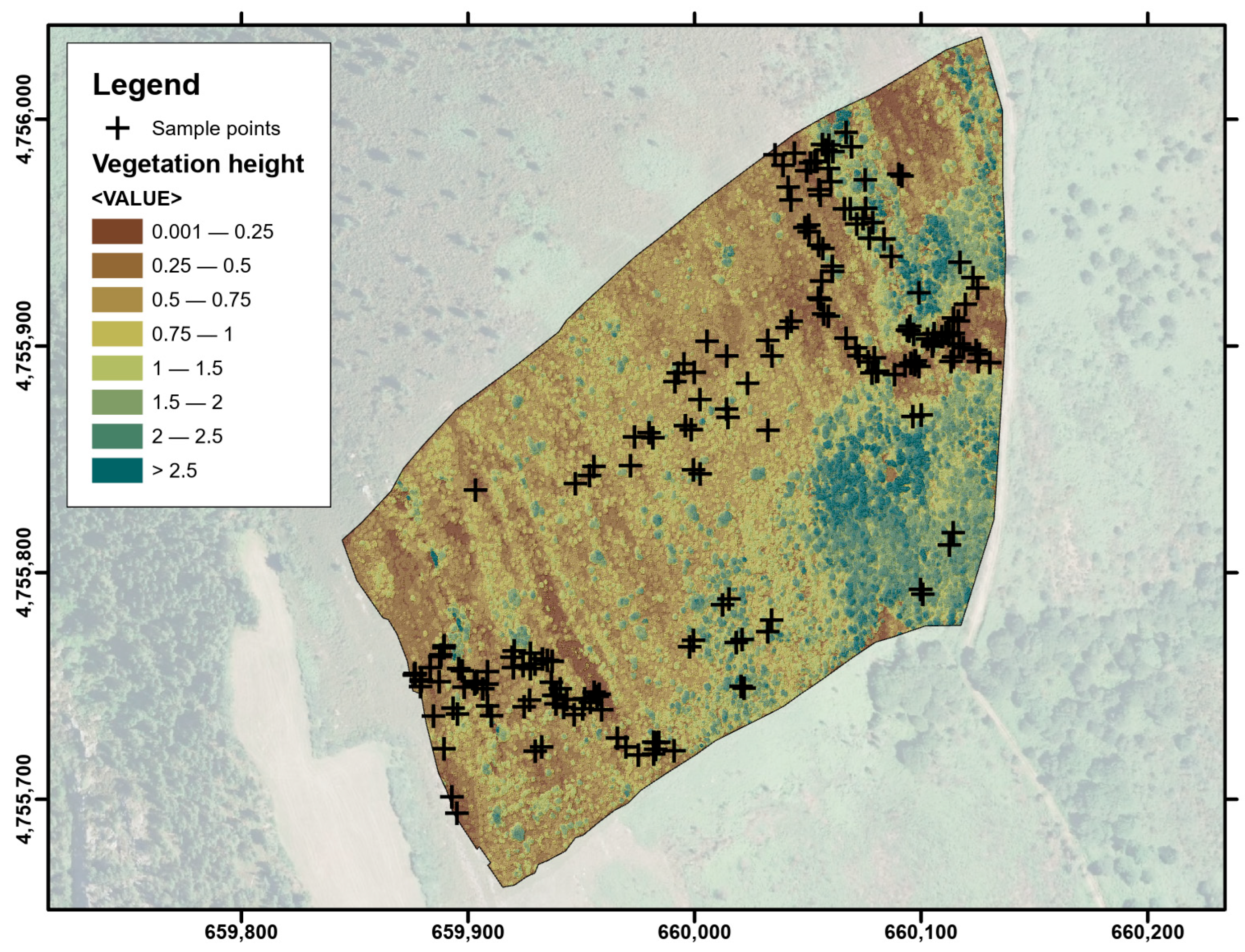
2.1. Study Area

The experiments were conducted in February 2019 in an area of 6.16 ha included in a plot burned by prescribed fire. The study area is located in the Serra de Ancares (Galicia, NW Spain, Figure 1) on a northeast slope of elevation ranging from 500 to 680 m.a.s.l. (the highest area in the SW of the slope and the lowest area in the NE). The slope percentages are quite evenly distributed, varying from 40% to 55% (mean 47%), with a few locations reaching slopes of up to 70% around several rocky ridges in the SW of the plot. As the area was included in a program of prescribed burns, a strip surrounding the area underwent the mechanical clearing of woody biomass to minimize the risk of wildfire spread during burning.
The pre-burn vegetation cover was dominated by several shrub communities with diverse cover and a variable height, along with scattered (frequently sub-metric) patches of low herbaceous (grasses) and more clumped patches of bracken (Pteridium aquilinum (L.) Kuhn in Kerst.). Hence, most of the area was covered by a mixture of dense, low (less than 1 m high) heaths (Calluna vulgaris (L.) Hull, Erica cinerea L., Erica umbellata Loefl. Ex. L., and Daboecia cantabrica (Huds.) K. Koch) along with other species in the families Leguminosae (Ulex galii Planch., Ulex europaeus L., and Pterospartum tridentatrum L.) and Cistaceae (Halimium lasianthum subsp. Alyssoides (Lam.) Greuter), frequently interspersed with bramble (Rubus sp.) in different proportions. The densest and highest (up to 2–3 m tall) shrub-dominated formation consisted of broom (Cytisus striatus (Hill) Rothm. and Cytisus multiflorus (L’Hér.) Sweet) or heath (Erica australis L. and Erica arborea L.) with variable proportions of the other above-mentioned species. These tall shrubs were more frequent in the lower part of the plot in dense formations, but scattered tall individuals, small clumps, and Erica arborea and E. australis were common through the area. At some points (rocky ridges and slopes, areas of shallow soil), bare ground/rock patches also occurred, particularly in the highest sectors of the plot.

2.2. Experimental Design and Analytical Overview

Taking into account the schedule of the prescribed burns, a series of UAV flights was planned in order to capture multi-seasonal and close-range remote sensing, and field surveys were conducted to capture composition and structure datasets of the shrub coverage before burning. Hence, a total of 204 field sampling points (locations for the acquisition of reference field data) were established for the measurement of vegetation height and the assignation of cover vegetation classes and fuel models, as detailed below.
Shrub height was computed using multitemporal digital photogrammetry 3D data from UAV RGB images, and reference values for validation were measured and geolocated in the field, trying to cover the diversity of shrub structure.
Five vegetation cover classes were considered in the vegetation classification scheme, considering the structure and assemblages of the main species (Table 1). The fuel model was also determined using the classification developed for shrubland communities in Galicia by Vega et al. [47], which distinguishes four custom models of woody shrub-dominated communities (Shrub-1 to Shrub-4) and two custom models of fern-dominated communities (Bracken-1 and Bracken-2), which, in the present study, were grouped into a single model (Bracken). The cited classification of fuel models for woody shrubland formations is based on the following two structural characteristics: the mean shrub height and the dead fine shrub load (Table 2).
The proposed fuel models for woody shrub-dominated communities represent an increasing gradient of fire virulence and, therefore, suppression effort from Shrub-1 to Shrub-4 [47] to consider the structural characteristics associated with each fuel model that affect the associated fire behavior.

2.3. RPAS Data Acquisition and Preprocessing

The airborne surveys providing the study data are summarized in Table 3. A total of four sets of images were acquired in three flights conducted on different dates, with the aim of capturing different phenological stages for multispectral image classification and pre- and post-fire stages for the digital surface and terrain model calculation, as detailed below. In all cases, vertical take-off and landing (VTOL) RPAS data were used, as they are particularly suited for the acquisition of small-area data in rough relief. For accurate georeferencing, a set of at least 8 ground control points (GCPs) was distributed across the flight area and their XYZ coordinates were measured with a Trimble Geo7X GNSS (Trimble Inc.TM, Westminster, CO, USA) with subsequent post-processing to obtain centimeter-accurate positions. Flights were conducted in automatic mode under the supervision of a ground pilot, following a previously defined single-grid flight plan.
The first flight survey was conducted on 18 April 2018, with the aim of capturing the early spring phenological stage of vegetation, using a lightweight RPAS DJI Phantom 3 Pro quadcopter equipped with the compact multispectral sensor Parrot Sequoia (Parrot Drone, SAS, Paris, France) with four 10-bit narrow spectral bands ranging across the visible-infrared spectrum (namely green, red, red edge, and near-infrared) and a synchronized irradiance + GNSS + IMU sensor. The sensor also included an RGB camera, which was not used at this stage. This flight was operated by researchers from the University of Santiago de Compostela. Two single-grid flight plans (due to aircraft autonomy constraints) were executed in autonomous mode at an average height above the ground of 80 m (as a compromise between a good data spatial resolution and the safety and yield of the mission), a minimum of 70% along- and across-track overlap, and with VLOS (Visual Line of Sight, Sydney, Australia) operation, providing 1026 acquisitions (four synchronized multispectral images for each acquisition) and an approximate Ground Sampling Distance of 7.5 cm.
The multispectral and RGB flight aimed at capturing the winter phenological stage of vegetation was conducted on 13 February 2019 with a lightweight RPAS ATYGES FV8 (ATYGES Ingeniería S.L., Málaga, Spain) operated by 3eData Ingeniería Ambiental S.L. The aircraft was equipped with a compact MicaSense RedEdge multispectral snapshot camera (MicaSense, Inc., Seattle, WA, USA) with five 16-bit narrow spectral bands covering the visible-infrared spectrum (namely blue, green, red, red edge, and near-infrared) and, as in the former, a synchronized irradiance + GNSS + IMU sensor. A single-grid flight plan was executed in autonomous mode with an average height above the ground of approximately 110 m, 80% and 70% along-track and across-track overlap, respectively, and VLOS (Visual Line of Sight) operation. The RPAS also acquired RGB images with a 24-megapixel camera (Sony Alpha ILCE 6300, Tokyo, Japan) with a fixed 16 mm lens. The multispectral sensor made 618 acquisitions (5 synchronized images for each acquisition), rendering an approximate average GSD of 9.4 cm, while the RGB camera acquired 256 images with an approximate average GSD of 3.5 cm.
A third flight was conducted on 15 March 2019, with the aim of capturing rmsepost-fire conditions (the prescribed fire occurred on 28 February 2019). This flight was conducted following approximately the same specifications as the pre-fire acquisition of 13 February 2019, capturing 287 RGB images at an approximate average GSD of 3.2 cm, with the aim of generating a reference DTM of the bare ground surface.
Each of the four sets of images were processed using SfM (Structure from Motion) 3D image reconstruction techniques, implemented with Pix4Dmapper V.4.5.6 software (© 2020 Pix4D SA, Prilly, Switzerland) using the standard settings recommended by the software documentation and introducing minor modifications or rematching when necessary. Hence, full-scale image keypoints, aerial grid matching, and 10,000 keypoints were set for the initial processing, whereas multiscale half image, the optimal point density, and a minimum of 3 matches were set for sparse point cloud generation. Finaly, a 7 × 7 matching window size was chosen for point cloud densification.
In the case of multispectral sets, images were spectrally calibrated against a reference panel with values of around 70% of diffuse reflectance in the visible-infrared spectrum after each flight, using the synchronized irradiance values captured by the sensor, thus enabling the generation of multispectral georeferenced image mosaics in absolute reflectance values.
RGB processing was conducted to generate georeferenced XYZ point clouds along with the corresponding orthomosaics and digital surface models. This information was basically used for reference purposes, to locate the field of training areas for classification (orthomosaics), and for the calculation of fuel height (point clouds).

2.4. Vegetation Height Estimation

The vegetation height was estimated by interpolating a normalized CHM and subtracting a reference digital terrain model. Among the different options tested, an SfM point cloud of the pre-fire vegetation canopy, an SfM post-fire point cloud (i.e., quasi-bare ground after the removal of most of the vegetation cover), and low-density LiDAR ground returns (to ensure ground references in the case of post-fire vegetation remains) were combined, as described below. Calculations were performed using the lidR package V. 4.1.2 [48] in R software [49], the QGIS 3.28 software, and FUSION 4.50 [50].
The 0.5 points/m2 LiDAR data from the Spanish National Plan for Aerial Orthophotography (PNOA -LiDAR) were obtained from the National Geographic Information Centre [51]. The point cloud was ground-filtered to extract a set of ground returns for the study area. This set of points was merged with the post-fire SfM point cloud and the ground filtering was repeated to ensure the removal of points corresponding to any vegetation remains in the post-fire dataset. The “groundfilter” FUSION algorithm was used with a cell size of 0.25 m and parameter values of g = −2.0, w = 2.5, a = 1.0, and b = 4.0 [50]. This point cloud was used to compute a DTM using a k-nearest neighbor approach with inverse-distance weighting (knnidw) interpolation, with a cell size of 0.10 m. The pre-fire point cloud heights minus the DTM (ground reference) were used for the calculation of a vegetation height point cloud, eventually allowing for the interpolation of the CHM by using a combination of the point-to-raster (p2r) and knnidw algorithms with a cell size of 0.10 m (see [48] for a more thorough description of the algorithms).
Accuracy was evaluated by comparing the estimated and measured values for the 204 points collected in the field. Field measurements were carried out during the non-growing period before the 13 February 2019 flight, with the aim of capturing the variety in vegetation heights in the study area. The height measurements from the 204 sample points ranged from 0 (bare ground) to 340 cm, with a mean value of 82 cm (s.d. 55.01 cm).
For each point, coordinates were measured with a GNSSTrimble Geo7X (Trimble Inc.TM, Westminster, CO, USA) RTK GNSS, and the vegetation height was measured with an extensible measuring rod. Due to the procedure used for collecting height shrub data, a maximum filter with a 3 × 3 cell kernel (i.e., 30 × 30 cm) was applied to the CHM prior to the extraction of the estimated shrub heights. The rationale of this calculation was to mimic the procedure of measuring heights in the field in the RPAS data height estimation, as the GNSS device often cannot be placed exactly on the axis of the shrub being measured and is placed at a certain distance away to allow for vertical positioning of the GNSS antenna pole. Considering the notes made by the field operators, the calculations were performed considering this maximum distance from the GNSS pole to the shrub top.
The goodness of the estimates was evaluated by the root mean squared error (RMSE) value and its relative value with respect to the mean height (RMSE%), as well as by graphical representations of the observed versus estimated heights by height classes and by fuel models, as height was the main driver for mapping the fuel models of this study using remote sensing [47].

2.5. Vegetation and Fuel Model Classification

Supervised automatic classification was used to discriminate between different vegetation classes and between fuel models following a Geographical Object-Based Image Analysis (GEOBIA) approach. The classification involved two stages and was conducted with Ecognition V. 10 software (© Trimble, Inc., Westminster, CO, USA) and R software packages, as detailed below. The segmentation or spatial clustering of image pixels was first carried out, with the aim of identifying meaningful segments or objects. Classification was then conducted on the basis of the statistical analysis of these objects and considering multispectral and multitemporal variables, vegetation indices, and 3D vegetation structure (i.e., the previously computed CHM). All the input datasets were resampled to a spatial resolution of 9.4 cm prior to the classification analyses.
In the first stage, we used a single segmentation level with the Ecognition V. 10 software, adjusting the parameters to the target objects, i.e., shrubs and, in general, small clusters of vegetation homogeneous in species composition and structure. The segmentation parameters were adjusted iteratively using a trial–error procedure by visual comparisons of segments against known reference areas in the image. Some degree of over-segmentation was accepted to enable the optimal delineation of the objects. Field measurement points included in objects with a very limited number of pixels were excluded from the analysis, so 180 objects were finally used.
The input features for the classification comprised multispectral and multitemporal bands and the NDVI value derived from these bands (mean, maximum, minimum, and standard deviation of the objects’ reflectance and NDVI computed from the spring and winter UAV flights) along with 3D vegetation features (mean, maximum, minimum, and standard deviation of the previously computed CHM), i.e., a total of 48 input features (mean, maximum, and minimum values and standard deviation of the green, red, red edge, and near-infrared bands and NDVI from the spring flight; mean, maximum, and minimum values and standard deviation of the blue, green, red, red edge, and near infrared bands and NDVI from the winter flight; and mean, maximum, and minimum values and standard deviation of the CHM for each object). The random forest (RF) algorithm was used because of its ability to deal with complex classification problems and its robustness against potential training issues such as imbalance or mislabeling [52].
Random-forest-based classification requires the number of trees and the number of randomized features selected in each split to be established. In this study, we used the “randomForest” V.4.7-1.1 package [53] in R software [49] to fit the RF models by establishing the number of trees as 1000, which is an appropriate value given the large number of features and observations, and optimizing the number of features selected in each split to improve the global accuracy of our classification. The predicted and reference values were used to construct the corresponding error matrix, and the global, user, and producer accuracy were calculated for each class along with the global Kappa index [54]. Moreover, 10-fold cross-validation was used to evaluate the model performance by repeating the process 1000 times and constructing a confusion matrix using the weighted classifications of out-of-bag observations. Finally, the importance of input features in terms of a reduction in Giny impurity was estimated by random permutation. As the number of pixels of each object ranged from 16 to 331 (mean value of 94.73), a weighted RF model was applied by relating a weight directly proportional to the pixel number to each object.
The RF analysis was repeated for the 180 field measurement points at the pixel level, in this case using the values of the bands, the associated NDVI, and the height estimated with the previously computed CHM in the specific pixel corresponding to the field measurement point, i.e., a total of 12 input features (green, red, red edge, and near-infrared values and NDVI value from the spring flight; blue, green, red, red edge, and near-infrared values and NDVI value from the winter flight, and CHM value for each pixel). This approach enabled a comparison of the accuracies of the object-based and pixel-based classifications. According to De Leeuw et al. [55], as the data used in the development of the random forest models in both methodologies (object-based and pixel-based) were not derived from independent samples, the comparison between the performance of each was carried out using McNemar’s chi-square test.

3. Results

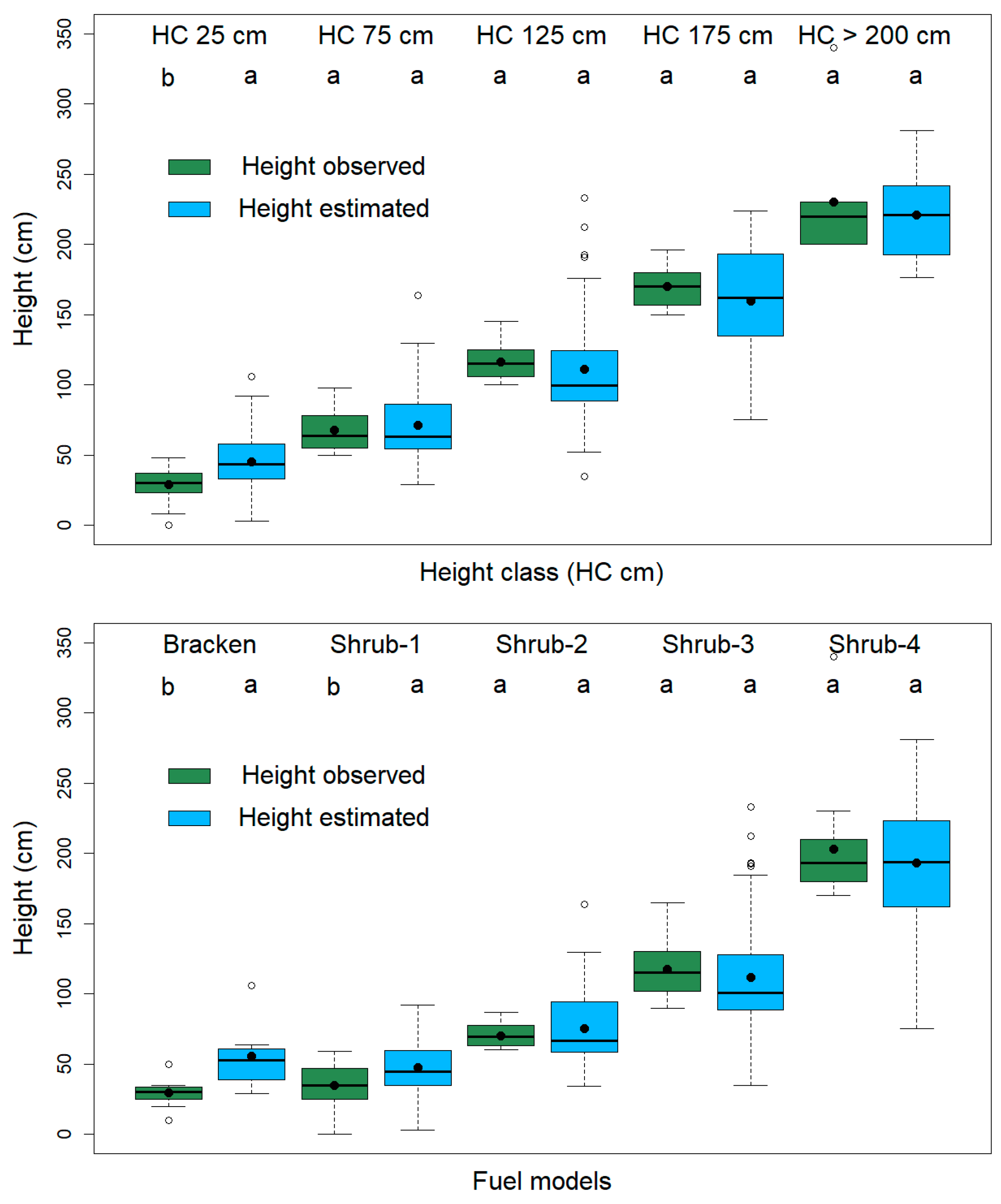
3.1. Height Estimation

The results of the spatial distribution of vegetation height estimation are graphically represented in Figure 2 and the frequencies of height values are summarized in Figure 3.
Most of the area was covered by vegetation lower than 1.0 m (Figure 3), with the maximum frequencies occurring in the interval of 0.5–0.75 m, with a mean height of 0.96 m. Shrubs higher than 2 m were located in the lower part of the slope (East in Figure 2, with a few peaks higher than 2.5) along with other isolated individuals scattered throughout the area.
The observed heights were plotted against the estimated values for the 204 field sampling points (Figure 4). The fitted linear model explains about 71% of the observed variability, with a root mean square error value of less than 0.3 m, representing around 36% of the measured height average. This model shows a slight tendency to overestimate height values above 0.75 m, although the value of the mean error (−0.039 m) seems to indicate a low level of bias.
As already mentioned, the classification of fuel models for woody shrubland formations in Galicia is based on two structural characteristics, the mean shrub height and the dead fine shrub load. However, to use the models to construct forest fuel maps derived from remotely sensed data, a dichotomous classification based solely on the mean shrub height was developed [47], so the estimated shrub heights derived from the CHM could be used to assign fuel models to the field measurement points applying the dichotomous key. Although a prior classification of the bracken-dominated shrubland communities and woody-dominated shrubland communities was necessary, if only the discriminant key for woody-dominated shrubland communities was used and the fuel models assigned in the field and those assigned using the CHM were compared, an overall accuracy of 64.90% was obtained with a Kappa index of 0.48, indicating a moderate level of agreement (from 0.41 to 0.60), in accordance with the classic scale proposed by Landis and Koch [54,56]. The values of the same index for each of the four fuel models indicated moderate to substantial agreement, except for the Shrub-2 fuel model, for which the user accuracy (0.31) and the Kappa index indicated a fair level of agreement (see Table 4).
Figure 5 shows box plots of the distribution of the observed and estimated values of the heights of the field samples for height classes defined in intervals of 50 cm and named by the class mark (Figure 5, top) and fuel models (Figure 5, bottom). The dispersion of the estimated height values is greater for all height classes than the dispersion of the field observed values, and significant differences (α = 5%) between the observed and estimated mean height are only observed in the lower height class (0–50 cm). The same is observed in the graph showing box plots of the observed and estimated height values for the fuel models, i.e., significant differences between the mean heights in the two lowest height fuel models (Bracken and Shrub-1).

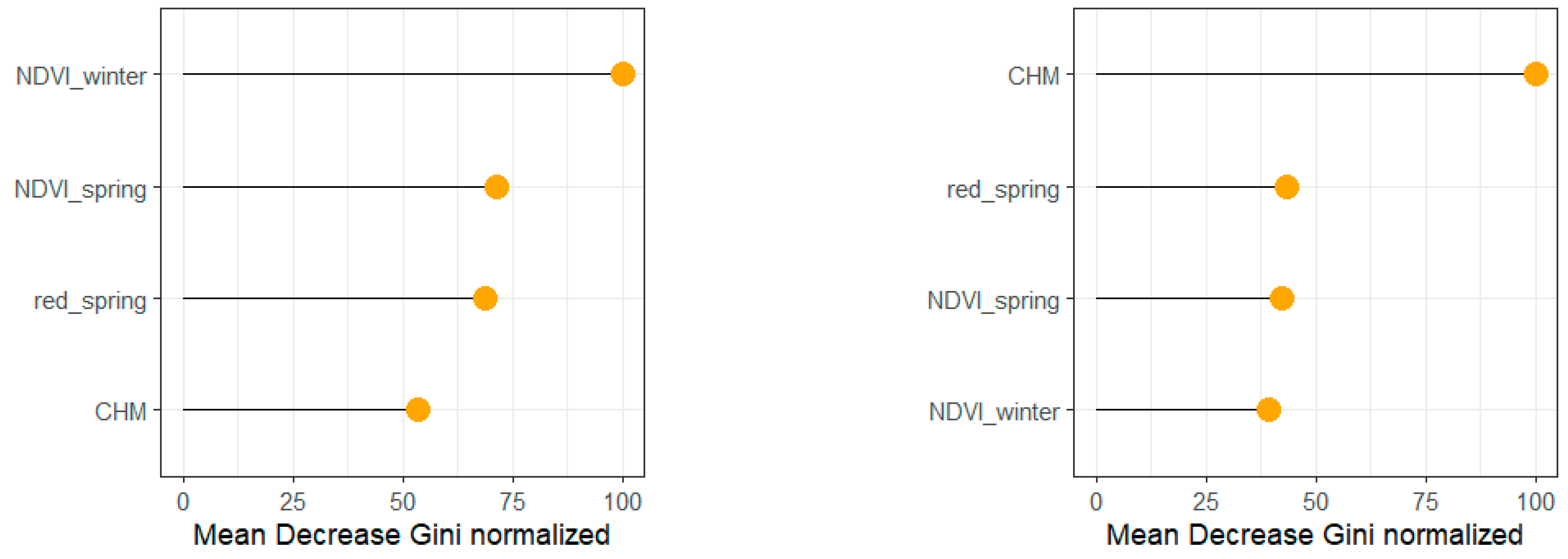
3.2. Pixel-Based Classification

For RF classification by vegetation class, the optimization of the number of features to select in each split indicated a value of 3 (25% of the 12 available features). The confusion matrix and a summary of the results and indices of the verification based on vegetation class are presented in Table 5. The global accuracy was 0.92, with a Kappa index of 0.90, indicating an almost perfect level of agreement (greater than 0.81), in accordance with the classic scale proposed by Landis and Koch [56]. The main discrepancies in the classification occurred when discriminating between the high shrub—heath and high shrub—broom classes.
The results of the cross-validation provided an overall accuracy of 91.13%, with a Kappa index of 0.88, and the most important features in the RF model were, in order of reduction in the Gini impurity value, the NDVI values of the winter and spring flights, the reflectance of the red band of the spring flight, and the height estimated with the CHM (Figure 6, left).
The optimization of the number of features to select in each split to improve the global accuracy of the RF classification by fuel model indicated a value of 2 (16.67% of the 12 available features). The confusion matrix obtained for fuel models and a summary of the results and indices of the verification by model are presented in Table 6. The global accuracy was 0.86, with a global Kappa index of 0.82, indicating almost perfect agreement. The main discrepancies occurred in the classification of the Shrub-2 fuel model, which the RF approach was not able to discriminate, classifying the nine observations between the Shrub-1 (four) and Shrub-3 (five) fuel models.
The results of the 10-fold cross-validation repeated 1000 times provided an overall accuracy percentage of 85.14%, with a Kappa index value of 0.80, showing that the height estimated with the CHM, the reflectance of the red band of the spring flight, the NDVI value of the spring flight, and the NDVI value of the winter flight were the most important features in the RF model in order of reduction in the Gini impurity value (Figure 6, right).

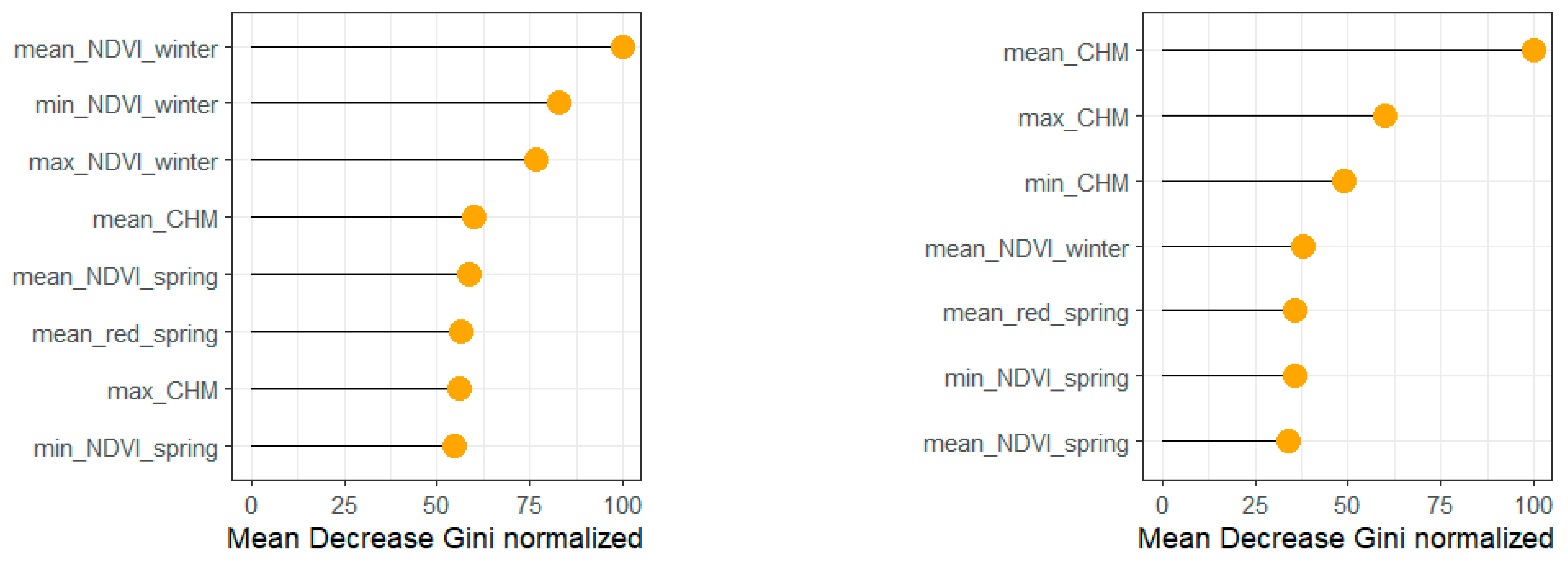
3.3. Object-Based Classification

The optimization of the number of features to be selected in each split to improve the overall accuracy of the RF classification of vegetation classes yielded a value of 4 (8.33% of the 48 available features). The confusion matrix and a summary of the results and indices of the discrimination by vegetation class are shown in Table 7. The global accuracy was 0.96, with a Kappa index of 0.95, also indicating, in this case, an almost perfect agreement [56]. The distribution of frequencies of the confusion matrix showed discrepancies only for discriminating between high shrub—heath and high shrub—broom, as in the pixel-based classification, and, to a much lesser extent, between the low shrub and bracken classes, probably due to the presence of mixtures and mosaics of these classes occurring according to the reference data.
The results of the 10-fold cross-validation repeated 1000 times provided an overall accuracy percentage of 95.08%, with a Kappa index value of 0.93, again indicating almost perfect agreement between the observed and estimated vegetation classes. Finally, analysis of the feature importance in the RF model indicated that the variables with the greatest weighting in the classification of vegetation classes were those related to the NDVI index values corresponding to the winter flight (mean, minimum, and maximum values) and, to a lesser extent, those from the spring flights (mean and minimum values), as well as those related to the height estimated by the CHM (maximum and mean values) and the mean value of the reflectance of the red band of the spring flight (Figure 7, left).
The overall accuracy of this method was higher than that of the pixel-based classification (0.96 vs. 0.92), and the McNemar’s chi-square test indicated significant differences in the performance between both RF-based methods used for the classification of vegetation classes (α = 5%).
Regarding the classification of the 180 objects using the random forest approach for the fuel models, the optimal number of features selected in each split was 4 (8.33% of the 48 available features). The confusion matrix and summary of the results and indices used to verify the fuel model are shown in Table 8. The a global accuracy of the classification was 0.93, with a Kappa index of 0.91, indicating an almost perfect agreement [54,56]. As with the RF pixel-based classification, the main discrepancies occurred in the classification of the fuel model Shrub-2, which the RF approach did not discriminate correctly, with an accuracy of 11.1% (one of nine observations correctly classified), classifying these observations among the fuel models Shrub-1 (55.5%) and Shrub-3 (33.3%).
The cross-validation provided an overall accuracy of 89.74%, with a Kappa index of 0.87, again indicating an almost perfect level of agreement [56] between the observed and estimated fuel models. The features with the greatest weighting in the classification based on fuel models were, in order of importance, those related to the height estimated by the CHM (mean, maximum, and minimum values) and, to a lesser extent, those related to the values of the NDVI index (mean and minimum values of the spring flight and mean value of the winter flight) and the mean value of the reflectance of the red band of the spring flight (Figure 7, right).
The McNemar’s chi-square test comparing the performances of the object-based and pixel-based RF classifications of fuel models indicated significant differences between the two classifications (α = 5%).
The mapping of the estimates obtained by the RF object-based classification applied to the 180 sample objects (we present just the classification with the best performance) is shown in Figure 8 for different vegetation classes (upper) and fuel models (lower).
Clearly, the most frequent vegetation class comprising the land cover in the area was low shrub. Other vegetation classes, such as high shrub—broom, were mainly clustered in the east part of the study area, corresponding to the lower part of the slope. The distribution of bare ground was more linear, following the rocky ridges in the higher sector of the slope (west of the plot). Bracken and high shrub—heath were more scattered and tended to be grouped in the south and east of the plot.
The study area was characterized by great heterogeneity in terms of fuel models. In addition, the patterns were highly mixed, as were the height classes (Figure 2). Clearly, the fuel models of the woody-dominated shrub communities (Shrub-1 to Shrub-4) covered a larger area than the model of the bracken-dominated communities. The most represented fuel model was Shrub-1, being the lowest in height. The tallest woody-dominated fuel models (Shrub 3 and Shrub 4) formed large patches in the east of the plot, while the largest areas occupied by Bracken were in the south center of the plot.

4. Discussion

Here, we present a methodology based on multitemporal 2D and 3D very high-resolution UAV data analysis for the characterization of heterogeneous shrub cover in a mountainous area, considering both structural aspects and vegetation and fuel composition. The originality of the work lies in the joint analysis of spectral responses in different phenological stages of the vegetation cover and in the comparison of 3D SfM point clouds before and after prescribed burning, which should, theoretically, enable a clear vision of the ground in the post-fire stage. Generally satisfactory results were obtained, despite some inaccuracies in identifying certain groups of species and fuel models in the vegetation and fuel classifications and the effect of outliers in shrub height estimation, as discussed below.
More specifically and regarding the height estimation, the RMSE was lower than 0.3 m. Notably, even the overall negative bias (−0.039 m) indicated slight overestimation, and a close look at the scatter plot and linear fit revealed that overestimation mainly applied to taller vegetation, whereas for lower vegetation, the estimated height values were similar to the measured values. This indicates an absence of systematic bias in the estimations.
One of the main challenges in DAP and ALS applications for vegetation surveys is the availability of accurate terrain surface data, i.e., digital terrain models, for estimating vegetation height [45,57], particularly in areas where steep slopes might hamper the interpolation of such models [58]. The present study is one of the few examples in which this issue is (at least theoretically) solved due to the information available after almost the complete removal of vegetation by prescribed burning. We assumed that the accuracy of the proposed methodology would mainly be related to the performance of the method in reconstructing the top of the vegetation and not to the DTM interpolation. Interestingly, the results did not show the general trend of severe underestimation of the vegetation height reported in other studies (even in studies using ALS), which has the advantage of pulse penetration in the canopy [45,59,60,61]. In the present study, we even observed a slight trend toward overestimation, particularly regarding the height of tall shrubs (higher than 0.75–1 m). The accuracy of the estimates obtained in the present work was, in some cases, higher than that in other studies involving high and dense shrubs/thickets and combining ground LiDAR returns and UAV DAP [33] or UAV ALS of dwarf vegetation marsh areas [59], with the latter having very low values of explained variability. In other cases, the accuracy of estimation was consistent with that obtained using only LiDAR data in shrublands [34], steppe meadows [60], or even in crops like maize [62]. In the study of steppe meadows, the main reason for the loss of accuracy was the difficulty in modeling the tops of vegetation rather than in the ground reference when using UAV LiDAR due to the probability of missing peaks of sharp vegetation profiles (probably isolated shrub peaks), especially in low vegetation. Similar results were obtained in recent studies comparing tree and shrubland heights (such as woody vegetation higher and lower than 5 m, respectively) from UAV DAP data in areas of sparse vegetation, with greater errors in modeling lower vegetation than higher vegetation [33].
Experiences in other environments such as tundra shrubland and isolated trees [25] yielded fewer errors using lower-height flights (45 m) and higher-resolution RGB (<1 cm) and overlap (in the order of 90%), with a consequent constraint in the flight area (less than 2 ha). In this case, the standard error of 8 cm for the estimation of the maximum height, along with the increase in the errors with degradation in the original resolution (standard errors of 23.2 cm for 1.5 cm DEM resolution), suggest the value of increasing the resolution of the image to improve the results. However, this approach must be considered carefully in each case, taking into account the dependence of the model performance in the cited work on the presence of small gaps in the canopy and the substantial decrease in yields when flights are conducted at a low altitude and speed.
Along with vertical structure and ground cover, species composition is a key feature involved in the ecology, biodiversity value, and fuel behavior of shrublands [63,64]. The automatic classification of shrublands based on remote sensing at different scales and from different data sources is an appealing approach that is widely reported in the literature. Mid-resolution multispectral satellite-based remote sensing in earth observation programs, such as Landsat or Sentinel, has been successfully used for the resource-efficient discrimination of some types of shrubland on a large scale [24,65,66]. Despite the advantage of the availability of free datasets and a wide spatial coverage, the low spectral and spatial resolution of the data hampers the development of classification schemes to the level of species or groups of species with similar environmental roles and/or fuel behavior. This difficulty could be addressed by improving the spectral resolution (e.g., by using hyperspectral imagery) or by increasing the spatial resolution of the images by using sensors with a higher IFOV and/or lower-altitude image registration (i.e., airborne or unmanned aircrafts). For example, hyperspectral airborne image classification enabled the discrimination of Calluna/Erica/Molinia heathland types, with overall accuracies ranging from 52 to 65% at an 18 m spatial resolution [67]. The ultra-high resolution of imagery acquired by UAVs enabled the use of simpler devices like RGB [68] or multispectral sensors [31]. In the former example, different components of wet heathlands and bog mosaics were discriminated at a spatial resolution of 2.5 cm, with an overall accuracy of 88%, whereas in the latter, different plots of low-density dry shrublands were classified, with an accuracy between 81.9% and 96.4%, from SfM point clouds with densities higher than 1000 points/m2 and low-density LiDAR data, to compute Canopy Height Models.
In the present study, we addressed the automated classification of UAV multispectral, multitemporal imagery combined with 3D vegetation structure data with a spatial resolution ranging from 3.2 to 9.4 cm. Taking into account the conspicuous phenological differences between the winter and spring spectral responses of some target species (namely bracken), we combined the data on both phenological stages, despite a temporal difference of one almost one year and the slightly different spatial and spectral resolutions of the images. Combining multispectral, multitemporal, and 3D vegetation cover information yielded good results (overall accuracy higher than 0.85 and Kappa indices higher than 0.80, regardless of the classification approach), despite the complexity of the classification problem. Regarding vegetation classification, the approach included classes that may be structurally similar, such as high shrub heath and broom, but with potential spectral differences, as well as other classes that may be spectrally similar but with different heights, such as various heath species and classes with a high greenness contrast throughout the year. The situation is even more complex for fuel model classification, as the same category includes communities dominated by different species (gorse, heath, and broom) that are only similar in terms of their range of heights and fine dead fuel loads. The vegetation cover was generally complete throughout most of the study area, except for some rocky areas and isolated patches of bare soil; isolated shrubs and small clumps of the same class were also very uncommon, with dense shrub formations and mixtures being more frequent and a transition between the targeted shrub classes being observed. Both factors could have hindered the discrimination of different classes and justified the use of high-spatial-resolution data to prevent the presence of pixel-level spectral mixtures in complex patterned vegetation [69,70], which somehow approach the scale of direct field surveys.
Regarding the classification methodology, the object-based approach produced slightly better results than the pixel-based approach for the discrimination of both vegetation classes and fuel models. However, the overall results indicated an almost perfect agreement in all cases, and the pixel-based methodology was simpler to apply and less conditioned by under- or over-segmentation and subjective parameterization. This approach may, therefore, be a useful option in this type of study. Similar results have been obtained when comparing the performances of these two methodologies for classifying different vegetation formations [71,72,73].
In the classification of the fuel models, neither of the two methodologies correctly discriminated the Shrub-2 model. This particularly applies to the pixel-based methodology, which did not correctly classify any of the nine samples in this group, erroneously assigning them either to the Shrub-1 model or to the Shrub-3 model. This could have been because the Shrub-1, Shrub-2, and Shrub-3 models had relatively overlapping height ranges, and distinction in the field is mainly due to differences in the fine dead fuel load, which is not adequately characterized by remotely sensed variables [74,75] such as those used in RF model fitting. However, the combination of CHM-derived structural data and multitemporal and multispectral data significantly outperformed the fuel model classification based solely on CHM information (Table 4), with an overall accuracy of 64.90% versus 92.78% for object-based classification and 86.11% for pixel-based classification.
From the point of view of the influence that the misclassification of fuel models can have on fuel management decision making, the most serious problems result from assigning a potentially less dangerous model in terms of fire behavior. In the confusion matrix, these situations correspond to the values shown above the diagonal and represent 5% and 8.3% of the total field observations for the object-based (Table 6) and pixel-based (Table 8) approaches, respectively.
The methodology tested here requires multitemporal datasets and the availability of a good-quality DTM. This may be particularly critical considering the relatively low yields in the UAV data acquisition and the difficulty in accurately reconstructing the ground surface when covered by a dense and continuous woody coverage. The first factor may restrict the application of the method to areas in the range from 20 to 200 ha [19], whereas the second may compromise the performance of the method (i.e., by decreasing the accuracy of the vegetation height estimation) or its applicability, owing to the need for data that are more expensive to acquire, like high-density LiDAR data. However, simple, accurate, and easily replicable methods, such as that proposed here, have great potential in several research topics, including wildfires, biomass, and biodiversity [76,77], or as a benchmark for down- or upscaling by integrating UAV data with satellite and ground surveys [78,79,80]. This method is also particularly promising in the current scenario of increasing the availability of very-high-resolution data in spatial data infrastructure and increasing the development and optimization of UAV and sensors [61,81]. The future development of this research may focus both on improving results (e.g., by the use of UAV aerial scanners to improve terrain modeling, fine-tuning flight height, and image overlaps) and on correcting some of the discrepancies in the classification of different classes. Regarding the latter, testing spectral responses during other phenological stages or on other sections of the electromagnetic spectrum, combined with the use of other AI/machine learning classification algorithms, may be useful.

5. Conclusions

A methodology using 3D, multitemporal, and multispectral UAV datasets to characterize shrubland vegetation is presented, focusing on structural and species composition from the point of view of their role as fuels in wildfires.
Shrub height is an essential variable for estimating fuel load, which is a key driver for predicting fire intensity, planning fuel management treatments, and assessing carbon content and CO2 fixation. The spatial distribution of fuels is also an essential driver, since it determines, to a great extent, fire behavior and dynamics, in combination with topographic and weather factors.
The main insights include the potential to estimate vegetation height with an admissible error (RMSE ≤ 0.3 m), although with a slight overestimation for the highest vegetation. In addition, we compared object-oriented and pixel-oriented classifications using the multispectral and canopy height model of shrubland cover, applying them to vegetation classes and to fuel models customized for the study area.
The results showed a better performance in the estimates of the object-based methodology, although the pixel-based classifications were also very successful and their application is simpler. The inclusion of multispectral information from two different stages in the vegetative development of the communities studied was key in the classifications, as demonstrated by the fact that the most important features were, in most cases, NDVI-derived statistics from both periods. In addition, conducting a post-fire flight allowed for the development of a more accurate DTM, which was also an important feature in all classifications.
The study findings are also promising, with great potential as a framework for other applications such as habitat monitoring or vegetation regeneration studies after natural or anthropogenic disturbances. Future challenges include the discrimination of vegetation types that are very similar both spectrally and structurally, considering the different phenological stages of their development (e.g., with potential improvements using advanced sensors, other flight height and image overlaps, and AI/machine learning classification algorithms), and the need to use highly accurate digital terrain models as a reference.

Author Contributions

Conceptualization, R.A.D.-V., C.A.-R., S.A.-P. and A.D.R.-G.; methodology, R.A.D.-V., C.A.-R., J.G.Á.-G. and A.D.R.-G.; formal analysis, R.A.D.-V., C.A.-R., J.G.Á.-G. and A.D.R.-G.; investigation, R.A.D.-V., C.A.-R., S.A.-P. and A.D.R.-G.; resources, R.A.D.-V., C.A.-R., S.A.-P., C.I.B.-H. and A.D.R.-G.; data curation, R.A.D.-V., C.A.-R., S.A.-P., J.G.Á.-G. and A.D.R.-G.; writing—original draft preparation, R.A.D.-V., C.A.-R., J.G.Á.-G. and A.D.R.-G.; writing—review and editing, R.A.D.-V., C.A.-R., S.A.-P., C.I.B.-H., J.G.Á.-G. and A.D.R.-G.; supervision, R.A.D.-V. and A.D.R.-G.; project administration, A.D.R.-G.; funding acquisition, A.D.R.-G. All authors have read and agreed to the published version of the manuscript.

Funding

This work was supported by the project: INIA-RTA2017-00042-C05 (VIS4FIRE) funded by the Spanish National Program of Research, Development and Innovation (Plan Estatal de I + D + i) co-financed by the European Regional Development Fund (ERDF) of the European Union.

Data Availability Statement

Data are unavailable due to privacy or ethical restrictions.

Acknowledgments

The authors would like to thank the Fire Prevention Service of the Xunta de Galicia and the EPRIF team of the MITECO located in Becerrea (Lugo), especially Horacio Vilor Rivero for carrying out the prescribed burning, which was essential for the development of the work presented here. The authors would also like to thank Mario López, from the UXAFORES group, for his essential collaboration in the field work.

Conflicts of Interest

The authors declare no conflicts of interest.

References

  1. Anthroecology Lab. Shrublands. Available online: https://anthroecology.org/anthromes/guide/shrublands/ (accessed on 4 February 2024).
  2. Gimingham, C.H. An Introduction to Heathland Ecology; Oliver & Boyd: Edinburgh, UK, 1975. [Google Scholar]
  3. Loidi, J.; Campos, J.A.; Haveman, R.; Janssen, J. Shrublands of temperate Europe. In Forests—Trees of Life; M. Goldstein, M.I., DellaSala, D.A., Eds.; Elsevier: Amsterdam, The Netherlands, 2020; Volume 3. [Google Scholar] [CrossRef]
  4. European Commission. Interpretation Manual of European Union Habitats—EUR 28; DG Environment. Nature ENV B.3; European Commission, 2013. Available online: https://www.mase.gov.it/sites/default/files/archivio/allegati/rete_natura_2000/int_manual_eu28.pdf (accessed on 13 March 2025).
  5. De Graaf, M.C.C.; Bobbink, R.; Smits, N.A.C.; Van Diggelen, R.; Roelofs, J.G.M. Biodiversity, vegetation gradients and key biogeochemical processes in the heathland landscape. Biol. Conserv. 2009, 142, 2191–2201. [Google Scholar] [CrossRef]
  6. Walmsley, D.C.; Delory, B.M.; Alonso, I.; Temperton, V.M.; Härdtle, W. Ensuring the Long-Term Provision of Heathland Ecosystem Services—The Importance of a Functional Perspective in Management Decision Frameworks. Front. Ecol. Evol. 2021, 9, 791364. [Google Scholar] [CrossRef]
  7. Fagúndez, J. Heathlands confronting global change: Drivers of biodiversity loss from past to future scenarios. Ann. Bot. 2013, 111, 151–172. [Google Scholar] [CrossRef]
  8. Piessens, K.; Honnay, O.; Hermy, M. The role of fragment area and isolation in the conservation of heathland species. Biol. Conserv. 2005, 122, 61–69. [Google Scholar] [CrossRef]
  9. Webb, N.R. The Traditional Management of European Heathlands. J. Appl. Ecol. 1998, 35, 987–990. [Google Scholar] [CrossRef]
  10. Wessel, W.; Tietema, A.; Beier, C.; Emmett, B.; Peñuelas, J.; Riis-Nielsen, T. A qualitative ecosystem assessment for different shrublands in Western Europe under impact of climate change. Ecosystems 2004, 7, 662–671. [Google Scholar] [CrossRef]
  11. EUNIS. Factsheet for European Dry Heaths. Available online: https://eunis.eea.europa.eu/habitats/10084 (accessed on 4 February 2024).
  12. Gómez-González, S.; Paniw, M.; Durán, M.; Picó, S.; Martín-Rodríguez, I.; Ojeda, F. Mediterranean Heathland as a Key Habitat for Fire Adaptations: Evidence from an Experimental Approach. Forests 2020, 11, 748. [Google Scholar] [CrossRef]
  13. Olmeda, C.; Šefferová, V.; Underwood, E.; Millan, L.; Gil, T.; Naumann, S. EU Action Plan to Maintain and Restore to Favourable Conservation Status the Habitat Type 4030 European Dry Heaths; European Commission: Brussels, Belgium, 2020. [Google Scholar]
  14. Millington, A.C.; Alexander, R.W. (Eds.) Vegetation Mapping in the Last Three Decades of the Twentieth Century. In Vegetation Mapping. From Patch to Planet; John Wiley & Sons Ltd.: Chichester, UK, 2000; pp. 321–332. [Google Scholar]
  15. Xie, Y.; Sha, Z.; Yu, M. Remote sensing imagery in vegetation mapping: A review. J. Plant Ecol. 2008, 1, 9–23. [Google Scholar] [CrossRef]
  16. Assiri, M.; Sartori, A.; Persichetti, A.; Miele, C.; Faelga, R.A.; Blount, T.; Silvestri, S. Leaf area index and aboveground biomass estimation of an alpine peatland with a UAV multi-sensor approach. GIScience Remote Sens. 2023, 60, 2270791. [Google Scholar] [CrossRef]
  17. de Castro, A.I.; Shi, Y.; Maja, J.M.; Peña, J.M. UAVs for Vegetation Monitoring: Overview and Recent Scientific Contributions. Remote Sens. 2021, 13, 2139. [Google Scholar] [CrossRef]
  18. Torresan, C.; Berton, A.; Carotenuto, F.; Di Gennaro, S.F.; Gioli, B.; Matese, A.; Miglietta, F.; Vagnoli, C.; Zaldei, A.; Wallace, L. Forestry applications of UAVs in Europe: A review. Int. J. Remote Sens. 2017, 38, 2427–2447. [Google Scholar] [CrossRef]
  19. Guerra-Hernández, J.; Díaz-Varela, R.A.; Álvarez-González, J.G.; González, P.M.R. Assessing a novel modelling approach with high resolution UAV imagery for monitoring health status in priority riparian forests. For. Ecosyst. 2021, 8, 61. [Google Scholar] [CrossRef]
  20. Manfreda, S.; McCabe, M.F.; Miller, P.E.; Lucas, R.; Madrigal, V.P.; Mallinis, G.; Dor, E.B.; Helman, D.; Estes, L.; Ciraolo, G.; et al. On the Use of Unmanned Aerial Systems for Environmental Monitoring. Remote Sens. 2018, 10, 641. [Google Scholar] [CrossRef]
  21. Mohsan, S.A.H.; Othman, N.Q.H.; Li, Y.; Alsharif, M.H.; Khan, M.A. Unmanned aerial vehicles (UAVs): Practical aspects, applications, open challenges, security issues, and future trends. Intelligent Service. Robotics 2023, 16, 109–137. [Google Scholar] [CrossRef] [PubMed]
  22. Detka, J.; Coyle, H.; Gomez, M.; Gilbert, G.S. A Drone-Powered Deep Learning Methodology for High Precision Remote Sensing in California’s Coastal Shrubs. Drones 2023, 7, 421. [Google Scholar] [CrossRef]
  23. Prošek, J.; Šímová, P. UAV for mapping shrubland vegetation: Does fusion of spectral and vertical information derived from a single sensor increase the classification accuracy? Int. J. Appl. Earth Obs. Geoinf. 2019, 75, 151–162. [Google Scholar] [CrossRef]
  24. Díaz Varela, R.A.; Ramil Rego, P.; Calvo Iglesias, S.; Muñoz Sobrino, C. Automatic habitat classification methods based on satellite images: A practical assessment in the NW Iberia coastal mountains. Environ. Monit. Assess. 2008, 144, 229–250. [Google Scholar] [CrossRef]
  25. Fraser, R.H.; Olthof, I.; Lantz, T.C.; Schmitt, C. UAV photogrammetry for mapping vegetation in the low-Arctic. Arct. Sci. 2016, 2, 79–102. [Google Scholar] [CrossRef]
  26. Moritake, K.; Cabezas, M.; Nhung, T.T.C.; Lopez Caceres, M.L.; Diez, Y. Sub-alpine shrub classification using UAV images: Performance of human observers vs DL classifiers. Ecol. Inform. 2024, 80, 102462. [Google Scholar] [CrossRef]
  27. Li, Z.; Ding, J.; Zhang, H.; Feng, Y. Classifying Individual Shrub Species in UAV Images—A Case Study of the Gobi Region of Northwest China. Remote Sens. 2021, 13, 4995. [Google Scholar] [CrossRef]
  28. Mücher, C.A.; Kooistra, L.; Vermeulen, M.; Borre, J.V.; Haest, B.; Haveman, R. Quantifying structure of Natura 2000 heathland habitats using spectral mixture analysis and segmentation techniques on hyperspectral imagery. Ecol. Indic. 2013, 33, 71–81. [Google Scholar] [CrossRef]
  29. Sankey, T.T.; McVay, J.; Swetnam, T.L.; McClaran, M.P.; Heilman, P.; Nichols, M. UAV hyperspectral and lidar data and their fusion for arid and semi-arid land vegetation monitoring. Remote Sens. Ecol. Conserv. 2018, 4, 20–33. [Google Scholar] [CrossRef]
  30. Sankey, J.B.; Sankey, T.T.; Li, J.; Ravi, S.; Wang, G.; Caster, J.; Kasprak, A. Quantifying plant-soil-nutrient dynamics in rangelands: Fusion of UAV hyperspectral-LiDAR, UAV multispectral-photogrammetry, and ground-based LiDAR-digital photography in a shrub-encroached desert grassland. Remote Sens. Environ. 2021, 253, 112223. [Google Scholar] [CrossRef]
  31. Carbonell-Rivera, J.P.; Torralba, J.; Estornell, J.; Ruiz, L.Á.; Crespo-Peremarch, P. Classification of Mediterranean Shrub Species from UAV Point Clouds. Remote Sens. 2022, 14, 199. [Google Scholar] [CrossRef]
  32. Gonzalez Musso, R.F.; Oddi, F.J.; Goldenberg, M.G.; Garibaldi, L.A. Applying unmanned aerial vehicles (UAVs) to map shrubland structural attributes in northern Patagonia, Argentina. Jt. Virtual Issue Appl. UAVs For. Sci. 2020, 1, 615–623. [Google Scholar] [CrossRef]
  33. Klouček, T.; Klápště, P.; Marešová, J.; Komárek, J. UAV-Borne Imagery Can Supplement Airborne Lidar in the Precise Description of Dynamically Changing Shrubland Woody Vegetation. Remote Sens. 2022, 14, 2287. [Google Scholar] [CrossRef]
  34. Estornell, J.; Ruiz, L.A.; Velázquez-Marti, B. Study of Shrub Cover and Height Using LIDAR Data in a Mediterranean Area. For. Sci. 2011, 57, 171–179. [Google Scholar] [CrossRef]
  35. Zhao, Y.; Liu, X.; Wang, Y.; Zheng, Z.; Zheng, S.; Zhao, D.; Bai, Y. UAV-based individual shrub aboveground biomass estimation calibrated against terrestrial LiDAR in a shrub-encroached grassland. Int. J. Appl. Earth Obs. Geoinf. 2021, 101, 102358. [Google Scholar] [CrossRef]
  36. Aicardi, I.; Dabove, P.; Lingua, A.M.; Piras, M. Integration between TLS and UAV photogrammetry techniques for forestry applications. IForest 2016, 10, 41–47. [Google Scholar] [CrossRef]
  37. Anderson, K.E.; Glenn, N.F.; Spaete, L.P.; Shinneman, D.J.; Pilliod, D.S.; Arkle, R.S.; McIlroy, S.K.; Derryberry, D.R. Estimating vegetation biomass and cover across large plots in shrub and grass dominated drylands using terrestrial lidar and machine learning. Ecol. Indic. 2018, 84, 793–802. [Google Scholar] [CrossRef]
  38. Tian, J.; Li, H.; Sun, X.; Zhou, Y.; Ma, W.; Chen, J.; Zhang, J.; Xu, Y. Quality assessment of shrub observation data based on TLS: A case of revegetated shrubland, Southern Qinghai-Tibetan Plateau. Land Degrad. Dev. 2023, 34, 1570–1581. [Google Scholar] [CrossRef]
  39. Zabihi, K.; Paige, G.B.; Wuenschel, A.; Abdollahnejad, A.; Panagiotidis, D. Increased understanding of structural complexity in nature: Relationship between shrub height and changes in spatial patterns. SCIREA J. Geosci. 2023, 7, 78–95. [Google Scholar] [CrossRef]
  40. Panagiotidis, D.; Abdollahnejad, A.; Slavík, M. 3D point cloud fusion from UAV and TLS to assess temperate managed forest structures. Int. J. Appl. Earth Obs. Geoinf. 2022, 112, 102917. [Google Scholar] [CrossRef]
  41. Alonso-Rego, C.; Arellano-Pérez, S.; Cabo, C.; Ordoñez, C.; Álvarez-González, J.G.; Díaz-Varela, R.A.; Ruiz-González, A.D. Estimating Fuel Loads and Structural Characteristics of Shrub Communities by Using Terrestrial Laser Scanning. Remote Sens. 2020, 12, 3704. [Google Scholar] [CrossRef]
  42. van Blerk, J.J.; West, A.G.; Smit, J.; Altwegg, R.; Hoffman, M.T. UAVs improve detection of seasonal growth responses during post-fire shrubland recovery. Landsc. Ecol. 2022, 37, 3179–3199. [Google Scholar] [CrossRef]
  43. Olsoy, P.J.; Zaiats, A.; Delparte, D.M.; Germino, M.J.; Richardson, B.A.; Roser, A.V.; Forbey, J.S.; Cattau, M.E.; Caughlin, T.T. Demography with drones: Detecting growth and survival of shrubs with unoccupied aerial systems. Restor. Ecol. 2024, 32, e14106. [Google Scholar] [CrossRef]
  44. Pérez-Luque, A.J.; Ramos-Font, M.E.; Tognetti Barbieri, M.J.; Tarragona Pérez, C.; Calvo Renta, G.; Robles Cruz, A.B. Vegetation Cover Estimation in Semi-Arid Shrublands after Prescribed Burning: Field-Ground and Drone Image Comparison. Drones 2022, 6, 370. [Google Scholar] [CrossRef]
  45. Riaño, D.; Chuvieco, E.; Ustin, S.L.; Salas, J.; Rodríguez-Pérez, J.R.; Ribeiro, L.M.; Viegas, D.X.; Moreno, J.M.; Fernández, H. Estimation of shrub height for fuel-type mapping combining airborne LiDAR and simultaneous colour infrared ortho imaging. Int. J. Wildland Fire 2007, 16, 341–348. [Google Scholar] [CrossRef]
  46. Streutker, D.R.; Glenn, N.F. LiDAR measurement of sagebrush steppe vegetation heights. Remote Sens. Environ. 2006, 102, 135–145. [Google Scholar] [CrossRef]
  47. Vega, J.A.; Álvarez-González, J.G.; Arellano-Pérez, S.; Fernández, C.; Cuiñas, P.; Jiménez, E.; Fernández-Alonso, J.M.; Fontúrbel, T.; Alonso-Rego, C.; Ruiz-González, A.D. Developing customized fuel models for shrub and bracken communities in Galicia (NW Spain). J. Environ. Manag. 2024, 351, 119831. [Google Scholar] [CrossRef]
  48. Roussel, J.R.; Auty, D. Airborne LiDAR Data Manipulation and Visualization for Forestry Applications. R Package Version 4.1.2. Available online: https://cran.r-project.org/package=lidR (accessed on 12 February 2024).
  49. R Core Team. R: A Language and Environment for Statistical Computing; R Foundation for Statistical Computing: Vienna, Austria; Available online: https://www.R-project.org/ (accessed on 4 February 2024).
  50. McGaughey, R.J. FUSION/LDV: Software for LIDAR Data Analysis and Visualization; USDA Forest Service; Pacific Northwest Research Station: Corvallis, OR, USA, 2023. [Google Scholar]
  51. CNIG. Centro de Descargas del CNIG (IGN). Available online: http://centrodedescargas.cnig.es (accessed on 5 February 2024).
  52. Mellor, A.; Boukir, S.; Haywood, A.; Jones, S. Exploring issues of training data imbalance and mislabelling on random forest performance for large area land cover classification using the ensemble margin. ISPRS J. Photogramm. Remote Sens. 2015, 105, 155–168. [Google Scholar] [CrossRef]
  53. Liaw, A.; Wiener, M. Classification and Regression by randomForest. R News 2002, 2, 18–22. [Google Scholar]
  54. Congalton, R.; Green, K. Assessing the Accuracy of Remotely Sensed Data: Principles and Practices, 1st ed.; CRC/Lewis Press: Boca Raton, FL, USA, 1999. [Google Scholar]
  55. De Leeuw, J.; Jia, H.; Yang, L.; Liu, X.; Schmidt, K.; Skidmore, A.K. Comparing accuracy assessments to infer superiority of image classification methods. Int. J. Remote Sens. 2006, 27, 223–232. [Google Scholar] [CrossRef]
  56. Landis, J.R.; Koch, G.G. The measurement of observer agreement for categorical data. Biometrics 1977, 33, 159–174. [Google Scholar] [CrossRef]
  57. Estornell, J.; Ruiz, L.A.; Velázquez-Martí, B.; Hermosilla, T. Analysis of the factors affecting LiDAR DTM accuracy in a steep shrub area. Int. J. Digit. Earth 2011, 4, 521–538. [Google Scholar] [CrossRef]
  58. Su, J.; Bork, E. Influence of Vegetation, Slope, and Lidar Sampling Angle on DEM Accuracy. Photogramm. Eng. Remote Sens. 2006, 72, 1265–1274. [Google Scholar] [CrossRef]
  59. Curcio, A.C.; Peralta, G.; Aranda, M.; Barbero, L. Evaluating the Performance of High Spatial Resolution UAV-Photogrammetry and UAV-LiDAR for Salt Marshes: The Cádiz Bay Study Case. Remote Sens. 2022, 14, 3582. [Google Scholar] [CrossRef]
  60. Zhao, X.; Su, Y.; Hu, T.; Cao, M.; Liu, X.; Yang, Q.; Guan, H.; Liu, L.; Guo, Q. Analysis of UAV lidar information loss and its influence on the estimation accuracy of structural and functional traits in a meadow steppe. Ecol. Indic. 2022, 135, 108515. [Google Scholar] [CrossRef]
  61. Rodríguez Dorribo, P.; Alonso Rego, C.; Díaz Varela, R.A. Shrub height estimation for habitat conservation in NW Iberian Peninsula (Spain) using UAV LiDAR point clouds. Eur. J. Remote Sens. 2024, 58, 2438626. [Google Scholar] [CrossRef]
  62. Li, W.; Niu, Z.; Chen, H.; Li, D.; Wu, M.; Zhao, W. Remote estimation of canopy height and aboveground biomass of maize using high-resolution stereo images from a low-cost unmanned aerial vehicle system. Ecol. Indic. 2016, 67, 637–648. [Google Scholar] [CrossRef]
  63. Casals, P.; Gabriel, E.; De Cáceres, M.; Ríos, A.I.; Castro, X. Composition and structure of Mediterranean shrublands for fuel characterization. Ann. For. Sci. 2023, 80, 23. [Google Scholar] [CrossRef]
  64. de Bello, F.; Lavorel, S.; Gerhold, P.; Reier, Ü.; Pärtel, M. A biodiversity monitoring framework for practical conservation of grasslands and shrublands. Biol. Conserv. 2010, 143, 9–17. [Google Scholar] [CrossRef]
  65. Demirbaş Çağlayan, S.; Leloglu, U.M.; Ginzler, C.; Psomas, A.; Zeydanlı, U.S.; Bilgin, C.C.; Waser, L.T. Species level classification of Mediterranean sparse forests-maquis formations using Sentinel-2 imagery. Geocarto Int. 2022, 37, 1587–1606. [Google Scholar] [CrossRef]
  66. Macintyre, P.; van Niekerk, A.; Mucina, L. Efficacy of multi-season Sentinel-2 imagery for compositional vegetation classification. Int. J. Appl. Earth Obs. Geoinf. 2020, 85, 101980. [Google Scholar] [CrossRef]
  67. Chan, J.C.-W.; Beckers, P.; Spanhove, T.; Borre, J.V. An evaluation of ensemble classifiers for mapping Natura 2000 heathland in Belgium using spaceborne angular hyperspectral (CHRIS/Proba) imagery. Int. J. Appl. Earth Obs. Geoinf. 2012, 18, 13–22. [Google Scholar] [CrossRef]
  68. Díaz-Varela, R.A.; Calvo Iglesias, S.; Cillero Castro, C.; Díaz Varela, E.R. Sub-metric analysis of vegetation structure in bog-heathland mosaics using very high resolution rpas imagery. Ecol. Indic. 2018, 89, 861–873. [Google Scholar] [CrossRef]
  69. Müllerová, J.; Gago, X.; Bučas, M.; Company, J.; Estrany, J.; Fortesa, J.; Manfreda, S.; Michez, A.; Mokroš, M.; Paulus, G.; et al. Characterizing vegetation complexity with unmanned aerial systems (UAS)—A framework and synthesis. Ecol. Indic. 2021, 131, 108156. [Google Scholar] [CrossRef]
  70. Simpson, G.; Nichol, C.J.; Wade, T.; Helfter, C.; Hamilton, A.; Gibson-Poole, S. Species-Level Classification of Peatland Vegetation Using Ultra-High-Resolution UAV Imagery. Drones 2024, 8, 97. [Google Scholar] [CrossRef]
  71. Duro, D.C.; Franklin, S.E.; Dubé, M.G. A comparison of pixel-based and object-based image analysis with selected machine learning algorithms for the classification of agricultural landscapes using SPOT-5 HRG imagery. Remote Sens. Environ. 2012, 118, 259–272. [Google Scholar] [CrossRef]
  72. Fu, B.; Wang, Y.; Campbell, A.; Li, Y.; Zhang, B.; Yin, S.; Xing, Z.; Jin, X. Comparison of object-based and pixel-based Random Forest algorithm for wetland vegetation mapping using high spatial resolution GF-1 and SAR data. Ecol. Indic. 2017, 73, 105–117. [Google Scholar] [CrossRef]
  73. Berhane, T.M.; Lane, C.R.; Wu, Q.; Anenkhonov, O.A.; Chepinoga, V.V.; Autrey, B.C.; Liu, H. Comparing pixel-and object-based approaches in effectively classifying wetland-dominated landscapes. Remote Sens. 2017, 10, 46. [Google Scholar] [CrossRef]
  74. Arellano-Pérez, S.; Castedo-Dorado, F.; López-Sánchez, C.; González-Ferreiro, E.; Yang, Z.; Díaz-Varela, R.; Álvarez-González, J.G.; Vega, J.A.; Ruiz-González, A.D. Potential of sentinel-2A data to model surface and canopy fuel characteristics in relation to crown fire hazard. Remote Sens. 2018, 10, 1645. [Google Scholar] [CrossRef]
  75. D’Este, M.; Elia, M.; Giannico, V.; Spano, G.; Lafortezza, R.; Sanesi, G. Machine learning techniques for fine dead fuel load estimation using multi-source remote sensing data. Remote Sens. 2021, 13, 1658. [Google Scholar] [CrossRef]
  76. Keerthinathan, P.; Amarasingam, N.; Hamilton, G.; Gonzalez, F. Exploring unmanned aerial systems operations in wildfire management: Data types, processing algorithms and navigation. International J. Remote Sens. 2023, 44, 5628–5685. [Google Scholar] [CrossRef]
  77. Sun, Z.; Wang, X.; Wang, Z.; Yang, L.; Xie, Y.; Huang, Y. UAVs as remote sensing platforms in plant ecology: Review of applications and challenges. J. Plant Ecol. 2021, 14, 1003–1023. [Google Scholar] [CrossRef]
  78. Fernández-Alonso, J.M.; Llorens, R.; Sobrino, J.A.; Ruiz-González, A.D.; Alvarez-González, J.G.; Vega, J.A.; Fernández, C. Exploring the potential of lidar and sentinel-2 data to model the post-fire structural characteristics of gorse shrublands in NW Spain. Remote Sens. 2022, 14, 6063. [Google Scholar] [CrossRef]
  79. Beltrán-Marcos, D.; Suárez-Seoane, S.; Fernández-Guisuraga, J.M.; Fernández-García, V.; Marcos, E.; Calvo, L. Relevance of UAV and sentinel-2 data fusion for estimating topsoil organic carbon after forest fire. Geoderma 2023, 430, 116290. [Google Scholar] [CrossRef]
  80. Riihimäki, H.; Luoto, M.; Heiskanen, J. Estimating fractional cover of tundra vegetation at multiple scales using unmanned aerial systems and optical satellite data. Remote Sens. Environ. 2019, 224, 119–132. [Google Scholar] [CrossRef]
  81. Morgan, G.R.; Hodgson, M.E.; Wang, C.; Schill, S.R. Unmanned aerial remote sensing of coastal vegetation: A review. Ann. GIS 2022, 28, 385–399. [Google Scholar] [CrossRef]
Figure 1. Location of the study area. The lower map shows the location in detail: Instituto Geográfico Nacional. Ministerio de Fomento. Gobierno de España.
Forests 16 00676 g001
Figure 2. Spatial distribution of vegetation height (CHM) and sampling points. Background image from CNIG. Instituto Geográfico Nacional. Ministerio de Fomento. Gobierno de España).
Forests 16 00676 g002
Figure 3. Distribution of shrub height in the study area according to the results of the CHM (frequencies expressed in pixels × 106). Blue and red lines represent the mean and median values, respectively.
Forests 16 00676 g003
Figure 4. Plot of observed versus estimated vegetation heights. The red line represents the linear relationship between the two types of values and the dashed line denotes the 1:1 (identity) line.
Forests 16 00676 g004
Figure 5. Box plots of observed and estimated vegetation heights for height classes (upper) and for fuel models (lower). Different letters (a, b) indicate significant differences between mean values (α = 5%) for each class or model. Black dots represent mean values.
Forests 16 00676 g005
Figure 6. Normalized values of the mean decrease in Gini impurity of the most important variables in the random forest models for the pixel-based classification for vegetation classes (left) and fuel models (right). Values represented with an orange circle. The variable with the highest importance has been assigned a value of 100.
Forests 16 00676 g006
Figure 7. Normalized values of the mean decrease in Gini impurity of the most important variables in the random forest models for the object-based classification for vegetation classes (left) and fuel models (right). Values represented with an orange circle. The variable with the highest importance has been assigned a value of 100.
Forests 16 00676 g007
Figure 8. Results of object-based random forest classification of vegetation classes (upper) and fuel models (lower). (Background image from CNIG. Instituto Geográfico Nacional. Ministerio de Fomento. Gobierno de España).
Forests 16 00676 g008
Table 1. Vegetation classes used in the study and their description.
Vegetation ClassDescription
High shrub—heathFormation of high and dense shrubs (>1 m height)
dominated by Erica australis and Erica arborea
High shrub—broom Formation of high, dense shrubs (>1 m height)
dominated by Cytisus spp.
Low shrubShrub formation diverse in coverage and low or dwarf size (<1 m height) dominated by different woody species (Erica cinerea, Calluna vulgaris, Pterospartum tridentatum, Halimium lasianthum, and Ulex gallii, among others) with a variable share of herbaceous species other than bracken (Pteridium aquilinum)
BrackenDense formations of Pteridium aquilinum
Bare groundAreas with low or no vegetation coverage
(rocky habitats and bare ground)
Table 2. Fuel model used in the study and their description according [47].
Fuel ModelDescription
Shrub-1Young shrub communities with low height (<60 cm) and low fuel loads or non-senescent communities dominated predominantly by Erica umbellata, E. mackaiana, or Cistus ladanifer.
Shrub-2 Shrub communities with relatively small mean heights (<90 cm), although higher than Shrub-1, but with much larger loads, especially of fine fuels (diameter < 0.6 cm).
Shrub-3Shrub communities with higher heights (ranging from 90 to 170) and fuel loads than the two previous ones and with the highest load of both live and dead fine fuels, with the latter representing about 40% of the total fine fuel load.
Shrub-4Adult communities mainly dominated by species of the genera Cytisus, Erica australis, or E. arborea and Ulex europaeus, which have the highest heights (>170 cm) and largest total and coarse fuel loads (diameter ≥ 0.6 cm).
BrackenDense formations of Pteridium aquilinum
Table 3. Flights and remote sensing datasets.
DateRPASSensorData Type
Acquisitions
Pixel Size (cm)Rationale
18 April 2018
(spring, pre-burn)
Phantom3 ProParrot
Sequoia
Four-band multispectral10267.5Vegetation and fuel classification
13 February 2019
(winter, pre-burn)
RPAS FV-8 AtygesSony Alfa 6300, Tokyo, JapanRGB2563.5Fuel height
13 February 2019
(winter, pre-burn)
RPAS FV-8 AtygesMicasense RededgeTM, Seattle, WA, USAFive-band multispectral6189.4Vegetation and fuel classification
15 March 2019 (early spring, post-burn)RPAS FV-8 AtygesSony Alfa 6300, Tokyo, JapanRGB2873.2Ground reference
Table 4. Confusion matrix and accuracy statistics (Pro. Acc.—producer accuracy and User Acc.—user accuracy), detailing different fuel models of woody-dominated shrubland communities and total frequencies of the classification based on heights estimated using the CHM (rows) vs. fuel models assigned in field (columns).
Estimated Fuel ModelObserved Fuel Model
Shrub-1Shrub-2Shrub-3Shrub-4TotalPro.
Acc.
User
Acc.
Shrub-115520220.680.79
Shrub-234130200.200.31
Shrub-3144819720.670.70
Shrub-400631370.840.62
Total19136950151
Table 5. Confusion matrix and accuracy statistics of the pixel-based random forest classification for vegetation classes (Pro. Acc.—producer accuracy and User Acc.—user accuracy).
Estimated
Vegetation Class
Observed Vegetation Class
High
Shrub—Heath
High
Shrub—Broom
Low ShrubBrackenBare GroundTotalPro.
Acc.
User
Acc.
High Shrub—Heath665200730.970.90
High Shrub—Broom 232100350.840.91
Low Shrub011900200.860.95
Bracken000303331.000.91
Bare Ground000019190.861.00
Total6838223022180
Table 6. Confusion matrix and accuracy statistics of the pixel-based random forest classification of the fuel models (Pro. Acc.—producer accuracy and User Acc.—user accuracy).
Estimated
Fuel Model
Observed Fuel Model
BrackenBare groundShrub-1Shrub-2Shrub-3Shrub-4TotalPro.
Acc.
User
Acc.
Bracken3030000331.000.91
Bare ground 0190000190.861.00
Shrub-10013400170.810.76
Shrub-200101020.000.00
Shrub-30025577710.950.80
Shrub-40000236380.840.95
Total30221696043180
Table 7. Confusion matrix and accuracy statistics of the object-based random forest classification for vegetation classes (Pro. Acc.—producer accuracy and User Acc.—user accuracy).
Estimated
Vegetation Class
Observed Vegetation Class
High
Shrub—Heath
High
Shrub—Broom
Low ShrubBrackenBare GroundTotalPro.
Acc.
User
Acc.
High Shrub—Heath675000720.990.93
High Shrub—Broom 133000340.870.97
Low Shrub002210231.000.96
Bracken000290290.971.00
Bare Ground000022221.001.00
Total6838223022180
Table 8. Confusion matrix and accuracy statistics of the object-based random forest classification for fuel models (Pro. Acc.—producer accuracy and User Acc.—user accuracy).
Estimated
Fuel Model
Observed fuel model
BrackenBare GroundShrub-1Shrub-2Shrub-3Shrub-4TotalPro.
Acc.
User
Acc.
Bracken3000000301.001.00
Bare ground 0220000221.001.00
Shrub-10015500200.940.75
Shrub-200110020.110.50
Shrub-30003604671.000.90
Shrub-40000039390.911.00
Total30221696043180
Disclaimer/Publisher’s Note: The statements, opinions and data contained in all publications are solely those of the individual author(s) and contributor(s) and not of MDPI and/or the editor(s). MDPI and/or the editor(s) disclaim responsibility for any injury to people or property resulting from any ideas, methods, instructions or products referred to in the content.

