Abstract
Timely and accurate information on forest composition is crucial for ecosystem conservation and management tasks. Information regarding the distribution and extent of forested areas can be derived through the classification of satellite imagery. However, optical data alone are often insufficient to achieve the required accuracy due to the similarity in spectral characteristics among tree species, particularly in mountainous regions. One approach to improving the accuracy of forest classification is the integration of auxiliary environmental data. This paper presents the results of research conducted in the Slyudyanskoye Forestry area in the Irkutsk Region. A dataset comprising 101 variables was collected, including Sentinel-2 bands, vegetation indices, and climatic, soil, and topographic data, as well as forest canopy height. The classification was performed using the Random Forest machine learning method. The results demonstrated that auxiliary environmental data significantly improved the performance of the tree species classification model, with the overall accuracy increasing from 49.59% (using only Sentinel-2 bands) to 80.69% (combining spectral data with auxiliary variables). The most significant improvement in accuracy was achieved through the incorporation of climatic and soil features. The most important variables were the shortwave infrared band B11, forest canopy height, the length of the growing season, and the number of days with snow cover.
1. Introduction
Information on the composition and spatial distribution of tree species in study areas is essential for sustainable forest management [1]. Timely monitoring of forest resources is crucial for modeling forest dynamics, fire risk assessment, forest inventories, and evaluating carbon stock [2]. However, up-to-date data of sufficient accuracy and completeness are not always available to researchers and decision-makers. Traditional methods of forest research are time-consuming and costly, which makes it difficult to acquire relevant data [3].
This study focuses on the Slyudyanskoye Forestry area in the Irkutsk Region, located along the shore of Lake Baikal. Inventory data for this area, which include information on the spatial distribution of tree species, are not always accessible to the scientific community and are outdated for part of the region due to the complex mountainous terrain, which complicates field surveys [4]. Meanwhile, the forests around Lake Baikal are experiencing the impacts of wildfires, insect damage, and the prohibition of sanitary logging. Multispectral remote sensing (RS) data, widely available from open sources with regular updates and different resolutions, can provide valuable information about forests. Analyzing satellite imagery is less expensive than field forest research and saves time by scaling the results to areas with similar characteristics. Sentinel-2 and Landsat 8–9 imagery, with resolutions of 10 and 30 m, respectively, have been frequently used for forest resource research in recent years [5,6]. Sentinel-2 satellite imagery includes several bands in the shortwave infrared and red edge spectra which enhance the differentiation of vegetation types [7]. Ma et al. [8] revealed the effectiveness of multispectral sensors in classifying four tree species using Sentinel-2 images. The fusion of different remote sensing data sources can improve results. For example, the fusion of WorldView-2/3 imagery with LiDAR, as shown in [9], led to improved classification accuracy when mapping urban forest tree species using deep learning techniques.
Classification methods rely on a training dataset as a base; a set of pre-labeled polygons on the image, each assigned to a corresponding land cover-type class. Machine learning plays a significant role in tree species classification. Studies have shown [10,11,12,13] that Random Forest (RF), support vector machine (SVM), gradient boosting (XGBoost, GBDT), k-nearest neighbors (K-NN), and Naive Bayes (NB) algorithms can effectively identify tree species based on spectral and textural features. Random Forest classifiers have been widely adopted due to their effectiveness in handling high-dimensional data and their robustness to overfitting. For example, Lim et al. [14] combined spectral information with crown texture and environmental variables to map five dominant tree species in North Korea, highlighting the importance of utilizing diverse data sources.
Multispectral imagery alone is not always sufficient for large-scale environmental studies [15,16]. Identifying tree species in images can be challenging due to the similarity in reflectance and surface texture among different species. Current remote sensing technologies do not always provide accurate results, particularly in mountainous forests with dense canopy cover and complex species composition. The difficulty of accessing certain forested areas further limits the ability to collect accurate data for training classification algorithms. One approach to improving the classification results of satellite data is to add supplementary data—such as vegetation indices, topographic characteristics, soil data, and meteorological maps—into the original set of spectral bands [17].
For example, in a study examining differences in tree species classification in the northern and southern regions of China, Zhang et al. utilized a dataset of Sentinel-2, Landsat-8, and Sentinel-1 imagery, vegetation indices, texture, and topographic features [18], with altitude identified as the most significant contributor to classification accuracy. You et al. [19] compared 16 different combinations of features for classifying forest tree species, including Sentinel-2 spectral reflectance, vegetation indices, texture, phenological information, topography, precipitation, air temperature, UV aerosol index, and NO2 concentration. Their findings revealed that topography, UV aerosol index, and phenological information were the most important features for classification, whereas commonly used textural features had limited impact on accuracy. Chiang and Valdez [20], in their classification of tree species in Mongolia within the Siberian taiga zone—a region with topographic, climatic, and species composition characteristics similar to the area of this study—found that topographic variables (elevation, slope, aspect, and curvature) were more important than multispectral data for classifying individual tree species (birch, cedar, and willow). However, topographic data alone were insufficient to achieve high classification accuracy. Xie et al. [21] demonstrated that using multiple input data types—spectral, textural, topographic, and canopy height—for an area in Inner Mongolia, China, significantly improved the accuracy of land cover and forest classification compared to using only spectral bands. In a comparison of various combinations of Sentinel-2 imagery, topographic data, and textural characteristics for tree identification in the Prahova Valley, Romania, Vorovencii [22] found that the best results were achieved by combining all data types. However, the contribution of textural characteristics was minimal, while the addition of topographic data (elevation, aspect, and slope) significantly improved accuracy. Among the spectral data, the most important bands were B11, B12, and B3. To map forests in a mountain range in southwest China, Zheng et al. [23] collected multimodal data, including Sentinel-2 optical images, Sentinel-1 radar images, textural features, and topographic and climatic data. The combination of these data types improved classification accuracy; the integration of SAR data enhanced the separation of conifers and hardwoods but reduced the accuracy of oak recognition. Topographic and climatic parameters were found to have notable influences on forest classification in mountainous areas.
Liu et al. [24] investigated the distribution of tree species in a mountain forest using Sentinel-2 imagery, vegetation indices, and topographic data. The highest classification accuracy was achieved with the Random Forest method applied to monthly datasets, with the most important features being the SWIR bands (B11, B12), the NDVI index, elevation, and slope. Topographic features were more effective in distinguishing deciduous species than coniferous ones. Wang et al. [25] combined spectral, phenological, textural, and topographic features to identify tree species in the Changbai Mountains. In their study, topographic variables, particularly elevation, were the most significant, while phenological features based on NDVI time series had limited impacts on the results. Li et al. [26] utilized seasonal Landsat composites, vegetation indices, mean temperature, precipitation, and topographic data to classify tree species in a mountainous region in southwestern China. The top 10 important attributes in their study included six vegetation indices, elevation, temperature, and precipitation.
Although previous studies have explored the use of auxiliary data to improve classification accuracy, the impact of each feature varies significantly across different regions and forest types, necessitating further investigation. Moreover, researchers have predominantly focused on combining satellite imagery with vegetation indices and topographic data, rarely incorporating soil data and typically limiting climatic variables to air temperature and precipitation. This study aims to evaluate the influence of a wide range of ecological variables on the accuracy of tree species classification in mountain forest ecosystems, including Sentinel-2 imagery, vegetation indices, topographic, climatic, and soil data, as well as forest canopy height. The primary objectives were the following: (1) to evaluate the impact of auxiliary data on tree species classification accuracy compared to using only multispectral satellite images, (2) to investigate the influence of auxiliary data on the accuracy of classifying different forest species, and (3) to map dominant tree species within the study area.
2. Materials and Methods
The Slyudyanskoye Forestry area in the Irkutsk Region was selected as the study area (Figure 1). Its area is 351 thousand hectares, including 299 thousand hectares of forested land, which is over 85% of the region’s total area [27]. According to the Forest Regulations [28], within the Slyudyanskoye Forestry area, pine covers 13.9 thousand ha, spruce—4.6 thousand ha, fir—22.3 thousand ha, larch—20.5 thousand ha, cedar—159.4 thousand ha, birch—34.1 thousand ha, and aspen—3.2 thousand ha. The forestry area‘s territory is situated along the southern edge of Lake Baikal and is characterized by a pronounced mountainous relief. The high percentage of forest cover, coupled with the presence of mountainous and relatively inaccessible areas, underscores the importance of refining forest classification in the study area.
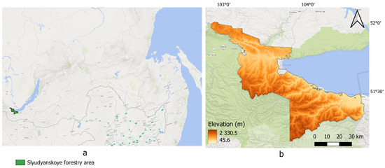
Figure 1.
Study area: (a) location of the Slyudyanskoye Forestry area; (b) map of the Slyudyanskoye Forestry area.
2.1. Data for Training
Sentinel-2 satellite imagery served as the base data in this study. Eleven main spectral bands (B1-B8, B8A, and B11-B12) were utilized for forest cover classification. Bands B9 and B10 were excluded from the classification process as they contain water vapor information and do not significantly contribute to the differentiation of tree species [29]. Band B1, which provides information on coastal aerosol concentration, was included due to the study area’s proximity to the Lake Baikal shoreline. This proximity can result in elevated aerosol levels, the concentration of which are influenced by the mountainous terrain of the area.
The auxiliary dataset comprised commonly used vegetation indices [30,31], soil, climatic, and topographic variables, and forest canopy height (Table 1).

Table 1.
List of auxiliary data types for classification.
2.1.1. Vegetation Indices
Vegetation indices were calculated using various combinations of Sentinel-2 bands, most frequently the red, near-infrared, and shortwave infrared bands, which have demonstrated a strong ability to identify tree species [44]. This capability stems from the fact that green vegetation absorbs red wavelengths and reflects infrared wavelengths, with absorption and reflection patterns varying among tree species due to differences in leaf structure and chlorophyll content. Shortwave infrared bands have longer wavelengths, so they propagate more effectively through the atmosphere, underscoring their high relevance in forest classification [45].
2.1.2. Soil Data
Soil parameters are directly related to the distribution of tree species in a given area. The proportions of sand, silt, and clay particles determine soil texture, which regulates water availability. Nitrogen and organic carbon content are indicators of soil quality and fertility, influencing productivity and large forest biomass stocks [46]. In this study, soil data were obtained from the ISRIC World Soil Information project website https://www.isric.org/ (accessed on 4 March 2025). The global SoilGrids datasets are presented as 250 m resolution raster maps that include information on soil chemical and physical properties. The values for each parameter are provided for six soil depth intervals from 0 to 200 cm (0–5 cm, 5–15 cm, 15–30 cm, 30–60 cm, 60–100 cm, and 100–200 cm). Soil density and composition parameters were selected as the mechanical properties for the study, while pH, nitrogen, and organic carbon content were chosen as the chemical properties. For each parameter, maps were downloaded for all six depth intervals.
2.1.3. Climate Data
Climate exerts a strong influence on the characteristics of forest vegetation. The growth and establishment of different tree species are closely related to their tolerance ranges for average annual precipitation and air temperature [46]. The primary climatic parameters selected for this study were minimum and maximum temperature and precipitation. These values were obtained from WorldClim datasets, which represent averaged values for the period 1970–2000 at a spatial resolution of 30 arcseconds. Additionally, Chelsa bioclimatic datasets were utilized [47,48]. These datasets provide globally interpolated data derived from key climatic variables (such as air temperature and precipitation) and are designed to model species distributions. They reflect annual trends (e.g., mean annual temperature), seasonality (annual range of temperature and precipitation), growing season parameters, and extreme or limiting environmental factors. The Chelsa datasets also include climatological norms for frost frequency, days of snow cover, and growing season characteristics (beginning, end, and duration). The values of Chelsa bioclimatic variables present averages for the period of 1981–2010.
2.1.4. Topographic Data
Topography significantly influences the distribution of forest tree species by creating unique conditions for their growth. As a result, topographic indicators are commonly used to refine the classification of tree species [49]. Slope gradient affects the angle of incidence of sunlight, and the aspect (the direction of the slope relative to the sides of light) determines the duration and intensity of sunlight exposure. Elevation is closely related to variations in climatic conditions such as temperature and humidity. In this study, topographic parameters, including elevation, slope, and shading, were calculated using the Copernicus Digital Elevation Model created in 2011–2015.
2.1.5. Forest Canopy Height
Tree height is a species-specific characteristic. Given that the study area contains both deciduous and coniferous tree species, canopy height data were incorporated into the analysis. A 10 m resolution forest canopy height map was obtained from the ETH Global Sentinel-2 Canopy Height dataset. This dataset provides tree height parameters derived through deep learning methods, combining data from GEDI LiDAR measurements and Sentinel-2 optical imagery. The integration of these datasets leverages the strengths of each: GEDI provides precise measurements of vertical forest structure, while Sentinel-2 offers extensive, high-resolution coverage of the Earth’s surface. This combination overcomes the limitations of using either dataset independently. The final map represents forest canopy height data on a global scale [50].
2.2. Model Evaluation
Classification was performed using the Random Forest machine learning method from the Python 3.12 scikit-learn library, which has demonstrated strong performance in solving similar problems [10,18,19,21,22,24]. The number of trees parameter was set to 500, while other algorithm parameters were retained at their default values. To evaluate the model’s performance, the values of overall accuracy across all classes, overall precision, recall, and F1 score [51] were employed. Validation samples were independently generated and annotated in QGIS 3.30 using the АсATaMa plugin and Google Earth imagery across the entire satellite image. This approach ensured spatial independence between the validation dataset and the training samples, thereby providing unbiased estimates.
To enhance model performance and assess the influence of different variables, the importance of each feature was calculated using the results of the internal Random Forest method (feature_importances). Feature importance was evaluated at each step of cross-validation using the K-Fold method. The dataset was divided into 10 parts, and the importance values for each feature were computed sequentially during each iteration. The mean importance values for each variable across all 10 iterations of cross-validation were used as the final results (Figure 2).
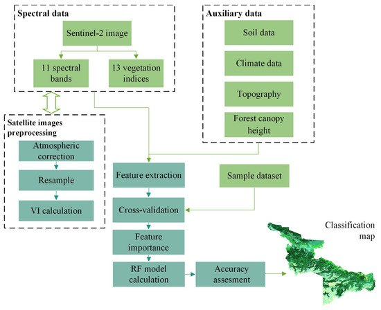
Figure 2.
Flowchart of the proposed method.
2.3. Features Combinations
Eight feature combinations were investigated in this study (Table 2). Models 1–6 compared the classification results using spectral bands alone and their alternating combinations with different auxiliary data. Model 7 included all collected features. The performance of all models was evaluated using the same validation dataset.
Table 2.
Features combination schemes.
2.4. Training Dataset
The 2009 Russian forest map with a resolution of 150 m [52] served as the basis for the training dataset. Based on an analysis of studies on the spectral reflectance of different tree species [7,53,54] and a visual comparison of the forest map with high-resolution Google Earth imagery, several key sites were selected for each of the seven tree species present in the Slyudyanskoye forestry area. The 2009 forest map provided baseline species information and each selected site was assessed using Google Earth imagery from 4 May 2019 to confirm the absence of disturbances since 2009 (e.g., logging, fires, or pest damage). Additionally, crown textures were visually compared to ensure consistency. Using the QGIS Semi-Automatic Classification Plugin, spectral characteristics were calculated for each site based on Sentinel-2 bands. The obtained spectra for all sites of the same species were compared, and sites with significant variations in spectral values were discarded as unreliable for that species.
After analyzing the set of collected key sites, it was decided to proceed with further annotation and classification into five species—pine, cedar, larch, fir, and birch. The spectral characteristics of aspen and spruce were found to be too similar to those of birch and fir, respectively. Additionally, the areas occupied by aspen and spruce within the forestry area were significantly smaller. As a result, additional data will be required in future studies to accurately delineate areas dominated by aspen and spruce.
Figure 3 illustrates the variation in reflectance across different species for Sentinel-2 bands. The derived reflectance values were used to annotate polygons representing areas occupied by the selected species. For this purpose, layers of Sentinel-2 band reflectance with the maximum differentiation between tree species (B7, B8, and B12) were used. In the QGIS Raster Calculator, a logical expression combining band thresholds for each species was constructed, and polygons corresponding to each species were delineated as bases on the resulting layer (Figure 4). Additionally, the general surface classes, including water, open ground, grass, and urban areas, were annotated.
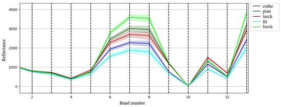
Figure 3.
Plot of tree species spectral characteristics by bands.
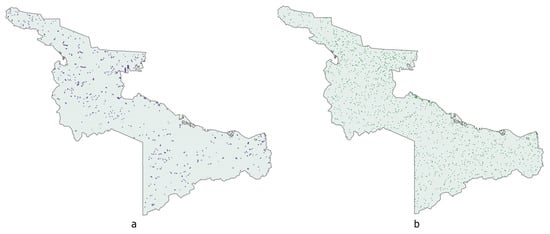
Figure 4.
Location of samples dataset: (a) training, and (b) test. The image illustrates the spatial distribution of the samples, not their area.
2.5. Data Preprocessing
The study area is situated at the intersection of three Sentinel-2 grid tiles. The original images were acquired from the Copernicus Hub on 5 July 2019 and subsequently processed using the Sen2Cor algorithm to perform base atmospheric corrections, resulting in Bottom-Of-Atmosphere (BOA) reflectance values for Sentinel-2 bands.
To cover the entire study area, the three original tiles were first merged band-by- band and then cropped to the forestry boundary in QGIS. Sentinel-2 bands were resampled to a 30 m resolution to reduce memory usage and improve processing efficiency. All auxiliary data were resampled to the same 30 m resolution using the k-nearest neighbors method via the ‘gdalwarp’ utility, ensuring that raster cells were aligned for precise overlap with the satellite band cells.
The values of all variables were normalized to the interval (0, 1). The initial datasets exhibited significant differences in absolute values: (0, 10,000) for Sentinel-2 bands, ranges (−2000, 30,000) and (−1, 1) for vegetation indices, and (0, 1000) for soil parameters. To address this imbalance, all indices were transformed using the method proposed for the Dynamic World global classification [55]. This approach involves logarithmic transformation and rescaling each dataset to a uniform interval (0, 1), ensuring the robustness of machine learning models during classification. Additionally, this transformation helped mitigate the influence of high-reflectance outliers in the spectral data distributions.
3. Results
The initial classification was performed using only Sentinel-2 bands. The overall accuracy was OAA = 49.59%, F1 score = 0.53 (Table 3). The most important bands for the model were the aerosol band B1 and shortwave infrared bands B11 and B12, followed by red B4 and red edge B5 and B6. The least important band was B8A (Figure 5a).
Table 3.
Overall model performance.
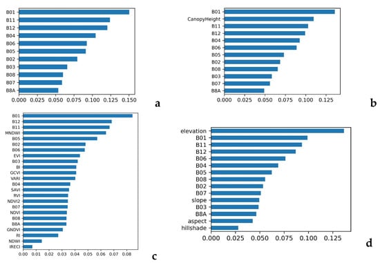
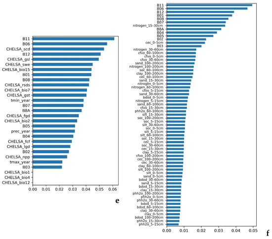
Figure 5.
Importance of features for different models: (a) S2 bands; (b) S2 + vegetation indices; (c) S2 + canopy height; (d) S2 + topography; (e) S2 + climate; and (f) S2 + soil.
The addition of vegetation indices did not improve the overall accuracy, and the accuracy of individual tree species recognition also remained unchanged. Among the vegetation indices, the Modified Normalized Difference Water Index (MNDWI) ranked fourth in importance, and the Extended Vegetation Index (EVI) ranked eighth. The remaining indices were ranked below the main bands and received similar importance scores. The water NDWI and the inverted red edge chlorophyll index IRECI were the least important (Figure 5c).
The inclusion of tree canopy height data increased the overall model accuracy by 2.27%. Among tree species, pine (+4.63%) and larch (+3.82%) showed the most significant improvements in accuracy, while birch exhibited a slight decrease (−2.51%) (Table 4). The relative importance of the optical bands remained consistent with the initial model, but the CanopyHeight feature emerged as the second most important feature (Figure 5b).
Table 4.
Overall accuracy by tree species.
The addition of topographic data increased the overall accuracy by 6.27% and the accuracy of tree species recognition by 4.69%. The most noticeable improvement was observed in the classification of fir, with an increase of 8.15%. In this model, elevation was the most important feature, highlighting the significance of incorporating topographic variables in classification, particularly for mountainous regions. The other topographic variables (slope, aspect, and hillshade) were less important than most of the primary Sentinel-2 bands (Figure 5d).
Climatic variables provided a substantial improvement in classification, increasing the overall accuracy to 67.38% compared to the initial 49.59% achieved with Sentinel-2 bands alone, so improvement was 17.79%. The average accuracy of tree species classification increased by 16.77%, from 51.63% to 68.4%. The most significant improvements were observed for pine (+29%), fir (+18.52%), and larch (+17.83%) (Figure 5). Among the climatic variables, the number of days with snow cover (CHELSA_scd), the length of the growing season (CHELSA_gsl), snow water equivalent (CHELSA_swe), and precipitation seasonality (CHELSA_bio15) were the most important. In contrast, annual mean air temperature (CHELSA_bio1), temperature seasonality (CHELSA_bio4), and annual precipitation (CHELSA_bio12) were the least important (Figure 5e).
The inclusion of soil features resulted in the largest increase in overall accuracy, with a 20.27% improvement from 49.59% to 69.86%. The accuracy of forest classification also increased by 15.79%. Among tree species, cedar (+23.86%) and pine (+23.53%) exhibited the most significant improvements (Figure 6). In this model, the B11, B6, and B12 bands were the most important, followed by other spectral bands, with nearly all soil parameters showing relatively low importance scores. Only two soil variables demonstrated importance scores comparable to the spectral data: total nitrogen at a depth of 15–30 cm (nitrogen_15–30 cm) and cation exchange capacity at a depth of 0–5 cm (cec_0–5 cm). Among all soil variables, total nitrogen at other depths, the volumetric fraction of coarse fragments (cfvo), and organic carbon content (soc) received the highest importance scores. In contrast, soil pH (phho), bulk density (bdod), and clay particle fraction (clay) showed lower importance (Figure 5f).
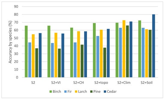
Figure 6.
Accuracy by tree species classes for different models.
The complete feature set, comprising 101 variables after integrating all auxiliary data, achieved an overall accuracy of 78.8% and a forest classification accuracy of 80.07%. This represents improvements of 29.21% and 28.44%, respectively, compared to the base set using only Sentinel-2 bands, and an increase of 8.94% and 12.65% compared to the set with soil variables, which previously demonstrated the highest accuracy. In this model, the B11 band was the most important feature, followed by forest canopy height (CanopyHeight), growing season length (CHELSA_gsl), and the number of days with snow cover (CHELSA_scd). The B12, B6, B8, and B8A bands, index MNDWI, and the average growing season temperature were among the top 10 most important features. Three bioclimatic parameters—CHELSA_bio1, CHELSA_bio4, CHELSA_bio12—showed the lowest importance, consistent with their performance in the S2 + Clim model. The water index NDWI also exhibited low importance (Figure 6).
As illustrated in the confusion matrices (Tables S1–S7), the addition of climatic features (Table S5) yielded maximum Producer’s Accuracy (PA) for three species classes—birch, larch, and cedar—and maximum User’s Accuracy (UA) for fir, larch, and pine. Soil variables (Table S6) produced maximum PA for fir and pine, and UA for cedar. The inclusion of topographic attributes (Table S4) produced maximum UA estimates for birch. As shown in Table S1, when using only Sentinel-2 bands, the highest number of misclassifications occurred between birch and larch and between fir and cedar due to the similarities in their spectral characteristics.
In the set of 101 features, three bioclimatic features exhibited significantly lower importance compared to the other variables; these features were removed, resulting in a refined set of 98 features for classification. This adjustment led to a slight improvement in model performance—overall accuracy increased by 1.89%, and tree species classification accuracy improved by 1–3%. Almost all species achieved accuracy levels above 80%, with the exception of birch, which had an accuracy of 79.92%. Cedar demonstrated the highest classification accuracy at 84.66%. Further attempts to remove additional features with minimal importance were unsuccessful, as they resulted in a decline in both overall accuracy and the accuracy of individual tree species.
Figure 6 and Figure 7 illustrate the importance of features across different models. The importance score of each feature is represented graphically, with higher scores indicating greater significance in the decision-making process. Sentinel-2 bands are labeled using a combination of the letter ‘B’ and their respective band numbers (e.g., B11 and B12). Soil variables are denoted by their parameter names followed by depth intervals in centimeters, indicating the average value for that specific depth range. For example, phh2o_15–30 cm represents the average soil pH value at a depth of 15 to 30 cm. CHELSA bioclimatic variables have a corresponding prefix in the name.
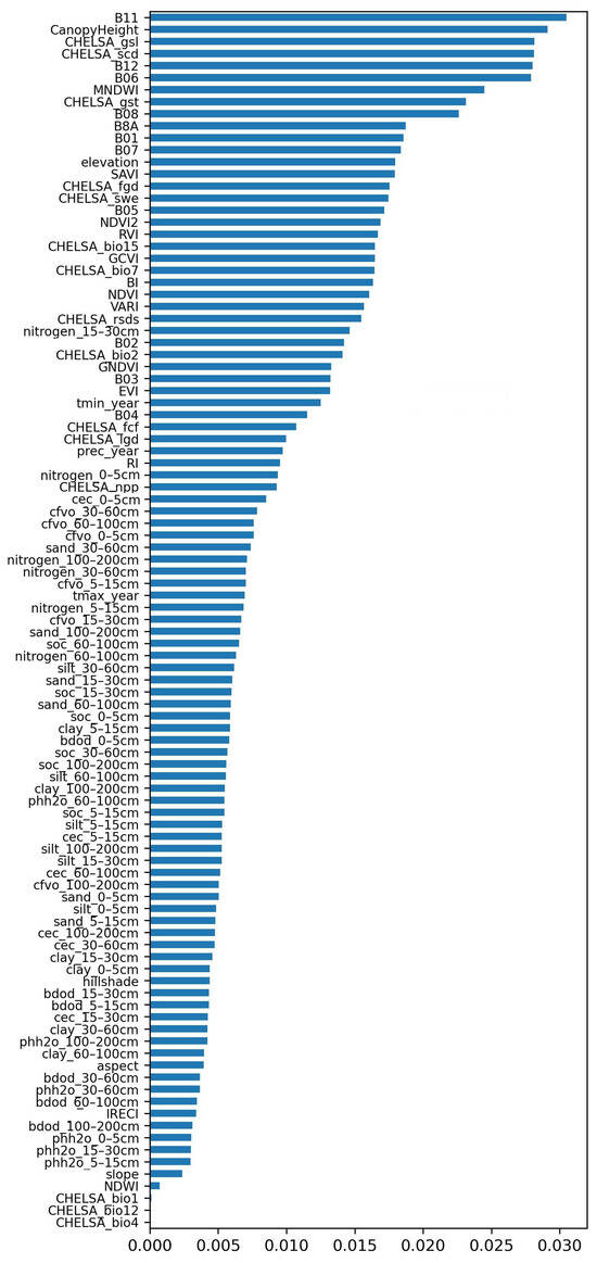
Figure 7.
Importance across all 101 features.
Figure 8 presents the final classification map depicting the distribution of tree species within the Slyudyanskoye forestry area. Birch is predominantly concentrated along the shoreline and riverbeds of Lake Baikal. Larch is primarily found in the northeastern part of the study area. Fir, pine, and cedar are distributed throughout the entire territory.
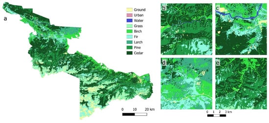
Figure 8.
Tree species distribution map: (a) the entire territory of the Slyudyanskoye forestry area; (b–e) enlarged spatial details of the map.
4. Discussion
4.1. Effect of Auxiliary Data on Model Performance
In this study, we evaluated the influence of various data types—spectral, topographic, climatic, and soil data—on the accuracy of tree species classification. Using only spectral bands, birch achieved a maximum accuracy of 65.69%, while pine recognition accuracy was significantly lower at 36.97%. From the Sentinel-2 spectral data, 13 vegetation indices were calculated which are associated with vegetation growth, water content, and chlorophyll concentration [56,57]. The bands most frequently used in the calculation of vegetation indices were green (B3), red (B4), and near-infrared (B8) bands. The addition of vegetation indices did not improve either overall accuracy or the accuracy of individual species classification. This finding aligns with the conclusions of previous studies [23,54,58] which suggest that a set of satellite bands, similar in quantity and spectral range to Sentinel-2 bands, may not always suffice for accurately distinguishing tree species.
In the models, we used two water indices—the NDWI and the modified MNDWI. The NDWI is calculated using bands B8 and B8A, while the MNDWI utilizes bands B3 and B11. Both indices serve as measures of vegetation moisture content [31,56]. In the full model with 101 features, the MNDWI ranked fifth in importance, whereas the NDWI was among the least important features, ranking fourth from the bottom. In our study area, coniferous species dominate, accounting for 78% of all tree species, with cedar comprising 80% of this group. The combination of green and SWIR bands proved more informative for interpreting moisture content in these species. This supports findings from previous research, which indicate that interspecies differences in coniferous tree species are most pronounced in the SWIR range [59,60]. Consequently, the MNDWI, which includes the SWIR band B11, received higher importance, while vegetation indices derived from other bands had a lesser impact.
The inclusion of forest canopy height data in [21] did not improve forest cover classification but enhanced accuracy for specific tree species (such as birch and Mongolian common pine). Our study yielded similar results, with a minimal increase in overall accuracy after adding canopy height data but notable improvements in the recognition accuracy of pine and larch. In the full feature set of 101 variables, CanopyHeight emerged as the most important feature. This underscores the significance of canopy height data in distinguishing tree species with marked differences in height. For instance, in our mountainous study area, pine reaches an average height of up to 38 m, larch up to 40 m, cedar up to 29 m, and birch up to 24 m [61].
Topographic features are widely recognized for their ability to enhance the accuracy of land cover classification [62]. Topography influences the natural distribution of tree species by regulating microclimate conditions and species habitats. Variations in elevation are directly linked to changes in light availability, precipitation, air pressure, and humidity levels. Our study area features mountainous terrain with elevation ranging from 580 to 2330 m above sea level. This significant elevation variation contributed substantially to the model’s performance, improving the recognition accuracy for fir, larch, and cedar. In the full feature set, elevation ranked seventh in importance, consistent with findings from other studies [63,64,65]. However, other topographic variables—slope, aspect, and shading—had lesser impacts on tree species recognition accuracy. This observation aligns with the results of [63] but contrasts with those of [65,66]. The relatively homogeneous dominance of cedar (62% of the study area) may explain this discrepancy, as it reduces the relationship between slope parameters and species distribution.
Climatic and soil attributes contributed similarly to the improvement in classification accuracy, highlighting the strong dependence of tree species distribution on temperature, precipitation, and soil type [46,67]. The extent of their contribution varied by species: climatic variables had a greater impact on the accuracy of larch and pine classification, while soil variables were more influential for birch and cedar. For fir, the effects of climatic and soil attributes were comparable (Table 4). These additional features significantly enhanced the accuracy of individual species classification. For instance, climatic variables increased the accuracy of pine classification by 29%, whereas the improvement for birch was only 3.77%. Similarly, soil attributes improved the recognition of cedar by 23.86% but had a lesser effect on larch, with an increase of only 6.37%.
The study area experiences a temperate continental climate characterized by stable snow cover during winter. This climatic condition underscored the high importance of variables such as the number of snow cover days and snow water equivalent. The significance of the precipitation seasonality (bio15) aligns with the findings from previous studies, which indicate that winter precipitation levels significantly influence the growing season in boreal forests [68,69,70]. Winter climatic conditions are particularly critical for cold-tolerant conifers; snow is one of the primary moisture resources in mountainous regions, mitigating the effects of low temperatures, their fluctuations, and needle desiccation. The diversity of tree species in the area (coniferous, deciduous, and deciduous conifers (larch)) further emphasize the importance of growing season length as a key variable.
The results confirmed the findings of [67], demonstrating that soil data enhance the performance of tree species classification models and facilitate the evaluation of relationships between soil characteristics and species distribution. For example, [71] revealed that competition between Scots pine and Norway spruce is influenced by soil texture, which in turn determines tree species composition. In our study area, nitrogen content, organic carbon, and soil texture characteristics (e.g., the volumetric fraction of coarse fragments) were the most important soil variables, while pH and bulk density were the least important. This contrasts with the findings of [67], where pH and density were the most significant predictors, likely due to differences in species composition and climatic conditions between study areas.
4.2. Limitations of the Method and Future Development
Due to the limited availability of training data only five out of the seven tree species present in the study area could be accurately identified. Further data collection, including field surveys, will be required to expand the training and validation dataset. This expansion will help to identify aspen and spruce in the spatial imagery and improve the accuracy of the classification of the five currently identified tree species.
During the training of the full set of 101 features, three bioclimatic variables exhibited minimal importance and their removal improved model performance. This suggest that, in our study area, the variables bio1, bio4, and bio12 have weak influences on the distribution of tree species, despite other studies [72,73,74] which have reported strong influences from these variables, particularly for pine and birch subspecies. Future research should include a more comprehensive analysis of climatic features by incorporating a broader range of bioclimatic variables at the preliminary stage. Cross-validation should then be performed to identify and remove variables with markedly lower importance compared to others.
The developed model can be adapted for tree species classification in other regions with similar environmental conditions, including location, climate, soil types, and species composition. However, the successful application of this model to new areas will depend on the availability of high-quality training data specific to those regions.
To further improve classification accuracy, future studies should consider incorporating textural characteristics, such as GLCM matrix parameters, which have proven effective in tree species classification [22,23]. Additionally, multi-temporal image series, when multiple satellite images of the same area captured at different times are used for model training, holds promise for enhancing classification performance. Finally, exploring more complex model architectures, such as ensemble methods, stacking, or deep learning models, could better capture spatial heterogeneities and further improve accuracy when combined with the auxiliary dataset proposed in this study.
5. Conclusions
In this study, we evaluated the impact of a wide range of environmental variables on the classification accuracy of tree species in mountain forest ecosystems. These included 18 climatic and 54 soil features. The integration of additional data types—such as vegetation indices, topographic features, climatic and soil variables, and forest canopy height—significantly improved classification accuracy. By incorporating these variables alongside spectral bands we increased the overall classification accuracy from satellite imagery by 31.1%, achieving a final accuracy of 80.69%. Among the auxiliary data, soil and climatic variables contributed the most to this improvement. In the full feature set, the most important variables were band B11, forest canopy height, and growing season length.
This study utilized a dataset collected for the first time to classify tree species in the Slyudyanskoye forestry area. All auxiliary data were obtained from open source global datasets. The resulting classification provides valuable insights into the spatial distribution and extent of different tree species, which are critical for effective forest resource monitoring and management.
Testing the model in other regions will help to assess its generalizability. If successful, the model can be adapted for use with diverse data sources and under varying environmental conditions, making it a valuable tool for large-scale forest monitoring. This adaptability could support broader efforts in sustainable forest management and biodiversity conservation.
Supplementary Materials
The following supporting information can be downloaded at: https://www.mdpi.com/article/10.3390/f16030487/s1, Table S1: Confusion matrix S2; Table S2: Confusion matrix S2+VI; Table S3: Confusion matrix S2+CH; Table S4: Confusion matrix S2+topo; Table S5: Confusion matrix S2+climate; Table S6: Confusion matrix S2+soil; Table S7: Confusion matrix all features.
Funding
The work was supported by the Ministry of Science and Higher Education of the Russian Federation, grant No. 075-15-2024-533 for implementation of Major scientific projects on priority areas of scientific and technological development (the project «Fundamental research of the Baikal natural territory based on a system of interconnected basic methods, models, neural networks and a digital platform for environmental monitoring of the environment»).
Data Availability Statement
The data presented in this study will be made available upon request from the corresponding author.
Conflicts of Interest
The authors declare no conflicts of interest.
References
- Pu, R. Mapping Tree Species Using Advanced Remote Sensing Technologies: A State-of-the-Art Review and Perspective. J. Remote Sens. 2021, 2021, 9812624. [Google Scholar] [CrossRef]
- Bonan, G.B. Forests, Climate, and Public Policy: A 500-Year Interdisciplinary Odyssey. Annu. Rev. Ecol. Evol. Syst. 2016, 47, 97–121. [Google Scholar] [CrossRef]
- Chiarucci, A.; Piovesan, G. Need for a Global Map of Forest Naturalness for a Sustainable Future. Conserv. Biol. 2020, 34, 368–372. [Google Scholar] [CrossRef] [PubMed]
- Bychkov, I.; Popova, A. Forest Landscape Model Initialization with Remotely Sensed-Based Open-Source Databases in the Absence of Inventory Data. Forests 2023, 14, 1995. [Google Scholar] [CrossRef]
- Talukdar, S.; Singha, P.; Mahato, S.; Shahfahad; Pal, S.; Liou, Y.-A.; Rahman, A. Land-Use Land-Cover Classification by Machine Learning Classifiers for Satellite Observations—A Review. Remote Sens. 2020, 12, 1135. [Google Scholar] [CrossRef]
- Nguyen, T.H.; Jones, S.; Soto-Berelov, M.; Haywood, A.; Hislop, S. Landsat Time-Series for Estimating Forest Aboveground Biomass and Its Dynamics across Space and Time: A Review. Remote Sens. 2019, 12, 98. [Google Scholar] [CrossRef]
- Grabska, E.; Hostert, P.; Pflugmacher, D.; Ostapowicz, K. Forest Stand Species Mapping Using the Sentinel-2 Time Series. Remote Sens. 2019, 11, 1197. [Google Scholar] [CrossRef]
- Ma, M.; Liu, J.; Liu, M.; Zeng, J.; Li, Y. Tree Species Classification Based on Sentinel-2 Imagery and Random Forest Classifier in the Eastern Regions of the Qilian Mountains. Forests 2021, 12, 1736. [Google Scholar] [CrossRef]
- Hartling, S.; Sagan, V.; Sidike, P.; Maimaitijiang, M.; Carron, J. Urban Tree Species Classification Using a WorldView-2/3 and LiDAR Data Fusion Approach and Deep Learning. Sensors 2019, 19, 1284. [Google Scholar] [CrossRef]
- Wang, J.; Bretz, M.; Dewan, M.A.A.; Delavar, M.A. Machine Learning in Modelling Land-Use and Land Cover-Change (LULCC): Current Status, Challenges and Prospects. Sci. Total Environ. 2022, 822, 153559. [Google Scholar] [CrossRef]
- Wessel, M.; Brandmeier, M.; Tiede, D. Evaluation of Different Machine Learning Algorithms for Scalable Classification of Tree Types and Tree Species Based on Sentinel-2 Data. Remote Sens. 2018, 10, 1419. [Google Scholar] [CrossRef]
- Axelsson, A.; Lindberg, E.; Reese, H.; Olsson, H. Tree Species Classification Using Sentinel-2 Imagery and Bayesian Inference. Int. J. Appl. Earth Obs. Geoinf. 2021, 100, 102318. [Google Scholar] [CrossRef]
- Bychkov, I.V.; Ruzhnikov, G.M.; Fedorov, R.K.; Popova, A.K.; Avramenko, Y.V. On Classification of Sentinel-2 Satellite Images by a Neural Network ResNet-50. Comput. Opt. 2023, 47, 474–481. [Google Scholar] [CrossRef]
- Lim, J.; Kim, K.-M.; Kim, E.-H.; Jin, R. Machine Learning for Tree Species Classification Using Sentinel-2 Spectral Information, Crown Texture, and Environmental Variables. Remote Sens. 2020, 12, 2049. [Google Scholar] [CrossRef]
- Liu, Y.; Gong, W.; Xing, Y.; Hu, X.; Gong, J. Estimation of the Forest Stand Mean Height and Aboveground Biomass in Northeast China Using SAR Sentinel-1B, Multispectral Sentinel-2A, and DEM Imagery. ISPRS J. Photogramm. Remote Sens. 2019, 151, 277–289. [Google Scholar] [CrossRef]
- Lechner, M.; Dostálová, A.; Hollaus, M.; Atzberger, C.; Immitzer, M. Combination of Sentinel-1 and Sentinel-2 Data for Tree Species Classification in a Central European Biosphere Reserve. Remote Sens. 2022, 14, 2687. [Google Scholar] [CrossRef]
- Xu, P.; Tsendbazar, N.-E.; Herold, M.; Clevers, J.G.P.W.; Li, L. Improving the Characterization of Global Aquatic Land Cover Types Using Multi-Source Earth Observation Data. Remote Sens. Environ. 2022, 278, 113103. [Google Scholar] [CrossRef]
- Zhang, J.; Li, H.; Wang, J.; Liang, Y.; Li, R.; Sun, X. Exploring the Differences in Tree Species Classification between Typical Forest Regions in Northern and Southern China. Forests 2024, 15, 929. [Google Scholar] [CrossRef]
- You, H.; Huang, Y.; Qin, Z.; Chen, J.; Liu, Y. Forest Tree Species Classification Based on Sentinel-2 Images and Auxiliary Data. Forests 2022, 13, 1416. [Google Scholar] [CrossRef]
- Chiang, S.-H.; Valdez, M. Tree Species Classification by Integrating Satellite Imagery and Topographic Variables Using Maximum Entropy Method in a Mongolian Forest. Forests 2019, 10, 961. [Google Scholar] [CrossRef]
- Xie, Z.; Chen, Y.; Lu, D.; Li, G.; Chen, E. Classification of Land Cover, Forest, and Tree Species Classes with ZiYuan-3 Multispectral and Stereo Data. Remote Sens. 2019, 11, 164. [Google Scholar] [CrossRef]
- Vorovencii, I. Assessing Various Scenarios of Multitemporal Sentinel-2 Imagery, Topographic Data, Texture Features, and Machine Learning Algorithms for Tree Species Identification. IEEE J. Sel. Top. Appl. Earth Obs. Remote Sens. 2024, 17, 15373–15392. [Google Scholar] [CrossRef]
- Zheng, P.; Fang, P.; Wang, L.; Ou, G.; Xu, W.; Dai, F.; Dai, Q. Synergism of Multi-Modal Data for Mapping Tree Species Distribution—A Case Study from a Mountainous Forest in Southwest China. Remote Sens. 2023, 15, 979. [Google Scholar] [CrossRef]
- Liu, P.; Ren, C.; Wang, Z.; Jia, M.; Yu, W.; Ren, H.; Xia, C. Evaluating the Potential of Sentinel-2 Time Series Imagery and Machine Learning for Tree Species Classification in a Mountainous Forest. Remote Sens. 2024, 16, 293. [Google Scholar] [CrossRef]
- Wang, M.; Li, M.; Wang, F.; Ji, X. Exploring the Optimal Feature Combination of Tree Species Classification by Fusing Multi-Feature and Multi-Temporal Sentinel-2 Data in Changbai Mountain. Forests 2022, 13, 1058. [Google Scholar] [CrossRef]
- Li, R.; Fang, P.; Xu, W.; Wang, L.; Ou, G.; Zhang, W.; Huang, X. Classifying Forest Types over a Mountainous Area in Southwest China with Landsat Data Composites and Multiple Environmental Factors. Forests 2022, 13, 135. [Google Scholar] [CrossRef]
- Popova, A.K.; Cherkasin, E.A.; Vladimirov, I.N. Forest Resources of the Baikal Region: Vegetation Dynamics Under Anthropogenic Use. Springer Proc. Earth Environ. Sci. 2019, 1, 96–106. [Google Scholar] [CrossRef]
- Forest Regulations Slyudyanskoye Forestry of the Irkutsk Region; Appendix 28 to the order of the Ministry of the Forestry Complex of the Irkutsk Region dated 28 January 2022 No. 91-7-mpr; Branch of FSBI “Roslesinforg Vostsiblesproekt”: Krasnoyarsk, Russia, 2021; p. 542.
- Campos-Taberner, M.; García-Haro, F.J.; Martínez, B.; Izquierdo-Verdiguier, E.; Atzberger, C.; Camps-Valls, G.; Gilabert, M.A. Understanding Deep Learning in Land Use Classification Based on Sentinel-2 Time Series. Sci. Rep. 2020, 10, 17188. [Google Scholar] [CrossRef]
- Wang, X.; Zhang, C.; Qiang, Z.; Xu, W.; Fan, J. A New Forest Growing Stock Volume Estimation Model Based on AdaBoost and Random Forest Model. Forests 2024, 15, 260. [Google Scholar] [CrossRef]
- Yuan, X.; Liu, S.; Feng, W.; Dauphin, G. Feature Importance Ranking of Random Forest-Based End-to-End Learning Algorithm. Remote Sens. 2023, 15, 5203. [Google Scholar] [CrossRef]
- Rouse, J.W.; Haas, R.H.; Schell, J.A.; Deering, D.W. Monitoring Vegetation Systems in the Great Plains with ERTS; NASA Special Publication; NASA: Washington, DC, USA, 1974. [Google Scholar]
- Baret, F.; Guyot, G. Potentials and Limits of Vegetation Indices for LAI and APAR Assessment. Remote Sens. Environ. 1991, 35, 161–173. [Google Scholar] [CrossRef]
- McFEETERS, S.K. The Use of the Normalized Difference Water Index (NDWI) in the Delineation of Open Water Features. Int. J. Remote Sens. 1996, 17, 1425–1432. [Google Scholar] [CrossRef]
- Escadafal, R.; Huete, A.R. Étude Des Propriétés Spectrales Des Sols Arides Appliquée À L’Amélioration Des Indices De Végétation Obtenues Par Télédétection. Comptes Rendus Acad. Sci. 1991, 312, 1385–1391. [Google Scholar]
- HUETE, A.; LIU, H. A Feedback Based Modification of the Ndvi to Minimize Canopy Background and Atmospheric Noise. IEEE Trans. Geosci. Remote Sens. 1995, 33, 814. [Google Scholar]
- Gitelson, A.A.; Merzlyak, M.N. Remote Sensing of Chlorophyll Concentration in Higher Plant Leaves. Adv. Sp. Res. 1998, 22, 689–692. [Google Scholar] [CrossRef]
- Frampton, W.J.; Dash, J.; Watmough, G.; Milton, E.J. Evaluating the Capabilities of Sentinel-2 for Quantitative Estimation of Biophysical Variables in Vegetation. ISPRS J. Photogramm. Remote Sens. 2013, 82, 83–92. [Google Scholar] [CrossRef]
- Rußwurm, M.; Körner, M. Self-Attention for Raw Optical Satellite Time Series Classification. ISPRS J. Photogramm. Remote Sens. 2020, 169, 421–435. [Google Scholar] [CrossRef]
- Gitelson, A.A.; Viña, A.; Arkebauer, T.J.; Rundquist, D.C.; Keydan, G.; Leavitt, B. Remote Estimation of Leaf Area Index and Green Leaf Biomass in Maize Canopies. Geophys. Res. Lett. 2003, 30, 1248. [Google Scholar] [CrossRef]
- Du, Y.; Zhang, Y.; Ling, F.; Wang, Q.; Li, W.; Li, X. Water Bodies’ Mapping from Sentinel-2 Imagery with Modified Normalized Difference Water Index at 10-m Spatial Resolution Produced by Sharpening the Swir Band. Remote Sens. 2016, 8, 354. [Google Scholar] [CrossRef]
- Huete, A.R. A Soil-Adjusted Vegetation Index (SAVI). Remote Sens. Environ. 1988, 25, 295–309. [Google Scholar] [CrossRef]
- Gitelson, A.A.; Stark, R.; Grits, U.; Rundquist, D.; Kaufman, Y.; Derry, D. Vegetation and Soil Lines in Visible Spectral Space: A Concept and Technique for Remote Estimation of Vegetation Fraction. Int. J. Remote Sens. 2002, 23, 2537–2562. [Google Scholar] [CrossRef]
- Immitzer, M.; Vuolo, F.; Atzberger, C. First Experience with Sentinel-2 Data for Crop and Tree Species Classifications in Central Europe. Remote Sens. 2016, 8, 166. [Google Scholar] [CrossRef]
- Abdi, A.M. Land Cover and Land Use Classification Performance of Machine Learning Algorithms in a Boreal Landscape Using Sentinel-2 Data. GISci. Remote Sens. 2020, 57, 1–20. [Google Scholar] [CrossRef]
- Mensah, S.; Noulèkoun, F.; Dimobe, K.; Seifert, T.; Glèlè Kakaï, R. Climate and Soil Effects on Tree Species Diversity and Aboveground Carbon Patterns in Semi-Arid Tree Savannas. Sci. Rep. 2023, 13, 11509. [Google Scholar] [CrossRef] [PubMed]
- Karger, D.N.; Conrad, O.; Böhner, J.; Kawohl, T.; Kreft, H.; Soria-Auza, R.W.; Zimmermann, N.E.; Linder, H.P.; Kessler, M. Climatologies at High Resolution for the Earth’s Land Surface Areas. Sci. Data 2017, 4, 170122. [Google Scholar] [CrossRef]
- Karger, D.N.; Conrad, O.; Böhner, J.; Kawohl, T.; Kreft, H.; Soria-Auza, R.W.; Zimmermann, N.E.; Linder, H.P.; Kessler, M. Data from: Climatologies at High Resolution for the Earth’s Land Surface Areas [Dataset]. Dryad Digit. Repos. 2018. [Google Scholar] [CrossRef]
- Liu, M.; Liu, J.; Atzberger, C.; Jiang, Y.; Ma, M.; Wang, X. Zanthoxylum Bungeanum Maxim Mapping with Multi-Temporal Sentinel-2 Images: The Importance of Different Features and Consistency of Results. ISPRS J. Photogramm. Remote Sens. 2021, 174, 68–86. [Google Scholar] [CrossRef]
- Lang, N.; Jetz, W.; Schindler, K.; Wegner, J.D. A High-Resolution Canopy Height Model of the Earth. Nat. Ecol. Evol. 2023, 7, 1778–1789. [Google Scholar] [CrossRef]
- Olofsson, P.; Foody, G.M.; Herold, M.; Stehman, S.V.; Woodcock, C.E.; Wulder, M.A. Good Practices for Estimating Area and Assessing Accuracy of Land Change. Remote Sens. Environ. 2014, 148, 42–57. [Google Scholar] [CrossRef]
- Schepaschenko, D.G.; Shvidenko, A.Z.; Lesiv, M.Y.; Ontikov, P.V.; Shchepashchenko, M.V.; Kraxner, F. Estimation of Forest Area and Its Dynamics in Russia Based on Synthesis of Remote Sensing Products. Contemp. Probl. Ecol. 2015, 8, 811–817. [Google Scholar] [CrossRef]
- Persson, M.; Lindberg, E.; Reese, H. Tree Species Classification with Multi-Temporal Sentinel-2 Data. Remote Sens. 2018, 10, 1794. [Google Scholar] [CrossRef]
- Wang, M.; Zheng, Y.; Huang, C.; Meng, R.; Pang, Y.; Jia, W.; Zhou, J.; Huang, Z.; Fang, L.; Zhao, F. Assessing Landsat-8 and Sentinel-2 Spectral-Temporal Features for Mapping Tree Species of Northern Plantation Forests in Heilongjiang Province, China. For. Ecosyst. 2022, 9, 100032. [Google Scholar] [CrossRef]
- Brown, C.F.; Brumby, S.P.; Guzder-Williams, B.; Birch, T.; Hyde, S.B.; Mazzariello, J.; Czerwinski, W.; Pasquarella, V.J.; Haertel, R.; Ilyushchenko, S.; et al. Dynamic World, Near Real-Time Global 10 m Land Use Land Cover Mapping. Sci. Data 2022, 9, 251. [Google Scholar] [CrossRef]
- Gao, B. NDWI—A Normalized Difference Water Index for Remote Sensing of Vegetation Liquid Water from Space. Remote Sens. Environ. 1996, 58, 257–266. [Google Scholar] [CrossRef]
- Gao, S.; Yan, K.; Liu, J.; Pu, J.; Zou, D.; Qi, J.; Mu, X.; Yan, G. Assessment of Remote-Sensed Vegetation Indices for Estimating Forest Chlorophyll Concentration. Ecol. Indic. 2024, 162, 112001. [Google Scholar] [CrossRef]
- Wan, H.; Tang, Y.; Jing, L.; Li, H.; Qiu, F.; Wu, W. Tree Species Classification of Forest Stands Using Multisource Remote Sensing Data. Remote Sens. 2021, 13, 144. [Google Scholar] [CrossRef]
- Rautiainen, M.; Lukeš, P.; Homolová, L.; Hovi, A.; Pisek, J.; Mõttus, M. Spectral Properties of Coniferous Forests: A Review of In Situ and Laboratory Measurements. Remote Sens. 2018, 10, 207. [Google Scholar] [CrossRef]
- Hovi, A.; Raitio, P.; Rautiainen, M. A Spectral Analysis of 25 Boreal Tree Species. Silva Fenn. 2017, 51, 7753. [Google Scholar] [CrossRef]
- Shvidenko, A.; Schepaschenko, D.; Nilsson, S. Tables and Models of Growth and Productivity of Forests of Major Forest Forming Species of Northern Eurasia (Standard and Reference Materials); Federal Agency of Forest Management, International Institute for Applied Systems Analysis: Moscow, Russia, 2008; 886p. [Google Scholar]
- Lu, D.; Weng, Q. A Survey of Image Classification Methods and Techniques for Improving Classification Performance. Int. J. Remote Sens. 2007, 28, 823–870. [Google Scholar] [CrossRef]
- Abdollahnejad, A.; Panagiotidis, D.; Shataee Joybari, S.; Surový, P. Prediction of Dominant Forest Tree Species Using QuickBird and Environmental Data. Forests 2017, 8, 42. [Google Scholar] [CrossRef]
- Pfeffer, K.; Pebesma, E.J.; Burrough, P.A. Mapping Alpine Vegetation Using Vegetation Observations and Topographic Attributes. Landsc. Ecol. 2003, 18, 759–776. [Google Scholar] [CrossRef]
- Lan, G.; Hu, Y.; Cao, M.; Zhu, H. Topography Related Spatial Distribution of Dominant Tree Species in a Tropical Seasonal Rain Forest in China. For. Ecol. Manag. 2011, 262, 1507–1513. [Google Scholar] [CrossRef]
- Garzón, M.B.; Blazek, R.; Neteler, M.; de Dios, R.S.; Ollero, H.S.; Furlanello, C. Predicting Habitat Suitability with Machine Learning Models: The Potential Area of Pinus Sylvestris L. in the Iberian Peninsula. Ecol. Modell. 2006, 197, 383–393. [Google Scholar] [CrossRef]
- Rota, F.; Scherrer, D.; Bergamini, A.; Price, B.; Walthert, L.; Baltensweiler, A. Unravelling the Impact of Soil Data Quality on Species Distribution Models of Temperate Forest Woody Plants. Sci. Total Environ. 2024, 944, 173719. [Google Scholar] [CrossRef]
- Yun, J.; Jeong, S.; Ho, C.; Park, C.; Park, H.; Kim, J. Influence of Winter Precipitation on Spring Phenology in Boreal Forests. Glob. Change Biol. 2018, 24, 5176–5187. [Google Scholar] [CrossRef]
- Martin, J.; Looker, N.; Hoylman, Z.; Jencso, K.; Hu, J. Differential Use of Winter Precipitation by Upper and Lower Elevation Douglas Fir in the Northern Rockies. Glob. Change Biol. 2018, 24, 5607–5621. [Google Scholar] [CrossRef]
- Lukasová, V.; Bucha, T.; Mareková, Ľ.; Buchholcerová, A.; Bičárová, S. Changes in the Greenness of Mountain Pine (Pinus Mugo Turra) in the Subalpine Zone Related to the Winter Climate. Remote Sens. 2021, 13, 1788. [Google Scholar] [CrossRef]
- Levula, J.; Ilvesniemi, H.; Westman, C. Relation between Soil Properties and Tree Species Composition in a Scots Pine–Norway Spruce Stand in Southern Finland. Silva Fenn. 2003, 37, 205–218. [Google Scholar] [CrossRef][Green Version]
- Feng, J.; Wang, B.; Xian, M.; Zhou, S.; Huang, C.; Cui, X. Prediction of Future Potential Distributions of Pinus Yunnanensis Varieties under Climate Change. Front. For. Glob. Change 2023, 6, 1308416. [Google Scholar] [CrossRef]
- Xiao, X.; Wang, Q.; Guan, Q.; Zhang, Z.; Yan, Y.; Mi, J.; Yang, E. Quantifying the Nonlinear Response of Vegetation Greening to Driving Factors in Longnan of China Based on Machine Learning Algorithm. Ecol. Indic. 2023, 151, 110277. [Google Scholar] [CrossRef]
- Yang, Q.; Xiang, Y.; Li, S.; Zhao, L.; Liu, Y.; Luo, Y.; Long, Y.; Yang, S.; Luo, X. Modeling the Impacts of Climate Change on Potential Distribution of Betula Luminifera H. Winkler in China Using MaxEnt. Forests 2024, 15, 1624. [Google Scholar] [CrossRef]


Disclaimer/Publisher’s Note: The statements, opinions and data contained in all publications are solely those of the individual author(s) and contributor(s) and not of MDPI and/or the editor(s). MDPI and/or the editor(s) disclaim responsibility for any injury to people or property resulting from any ideas, methods, instructions or products referred to in the content. |
© 2025 by the author. Licensee MDPI, Basel, Switzerland. This article is an open access article distributed under the terms and conditions of the Creative Commons Attribution (CC BY) license (https://creativecommons.org/licenses/by/4.0/).