Abstract
Ecotones, the transitional zones between distinct habitats, are vital for ecosystem functioning and habitat diversity. Traditional management practices frequently create abrupt boundaries, leading to stressful conditions for organisms. To address this challenge, an underutilized land management technique called “edge feathering”, which involves gradual thinning of the canopy along the forest edge, has been introduced. This study, conducted at Holden Arboretum in Kirtland, Ohio, investigated the effects of edge feathering on light availability and understory plant diversity in edge feathered and control treatments. We calculated the coefficient of variation in light availability as light heterogeneity and plant diversity indices at the plot level. Edge feathering increased light heterogeneity by more than 2.5-fold. It also significantly increased biodiversity, yielding twice the species richness and approximately 1.5 times higher Shannon and Simpson’s Diversity (1/D) indices compared to unmanaged control plots. Furthermore, greater light heterogeneity exhibited a strong positive correlation with increased understory plant diversity. These effects were observed within just 3.5 years of implementation, underscoring the rapid and measurable benefits of edge feathering for plant community diversity. Our results further suggest the hypothesis that light heterogeneity might be an important driver of small-scale plant community diversity in this system, which could be tested directly in the future.
1. Introduction
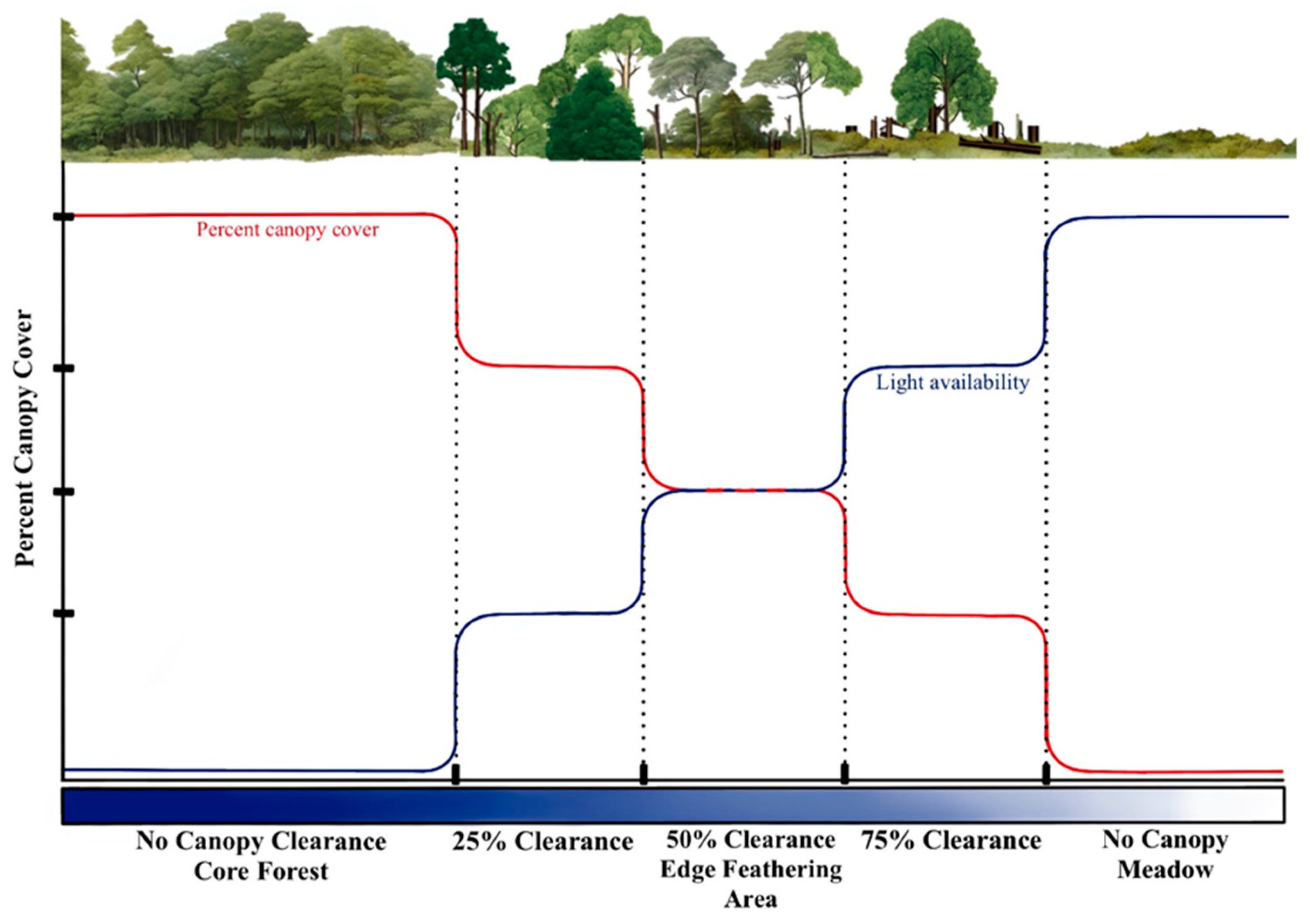
Ecotones, the transitional zones between different ecosystems, are widespread across various habitats and play a vital role in regulating the movement of organisms, energy, and matter [1,2,3]. For instance, while structurally distinct from forest interiors, forest-meadow ecotones resemble adjacent meadows, creating a dynamic mosaic of conditions that can facilitate and hinder species dispersal [4,5]. Effective forest management is essential to support the ecological functions of ecotones and conserve biodiversity, especially in regions heavily reliant on commercial forestry [1,6,7]. Traditional management of forest edges and adjacent fields often leaves abrupt transitions that, in effect, simplify habitat structures and reduce biodiversity [8]. A key consideration in these efforts is the width of the edge zone, which is crucial for maintaining interior habitat within forest fragments [9]. A wider and more gradual edge zone may reduce disruptive edge effects such as increased light, wind exposure, and temperature variation that alter the microclimate of the core habitat [8,10]. Edge feathering, a management technique that gradually transitions from forest to open habitat through selective tree removal, has emerged as a promising strategy for creating more complex and diverse edge environments [11] (Figure 1).
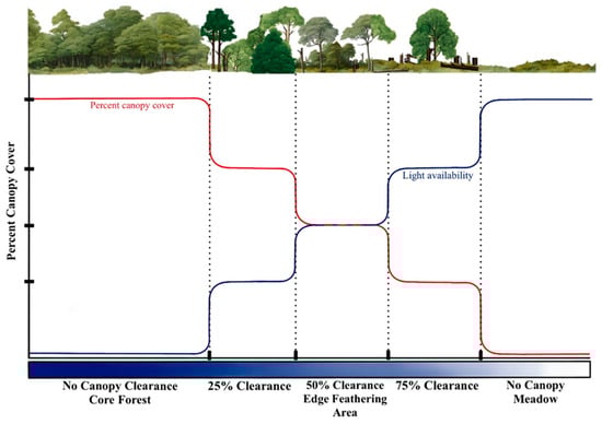
Figure 1.
Conceptual figure of how light availability changes with percent canopy cover in forest meadow ecotone subjected to edge feathering treatment.
Edge feathering may significantly impact overstory transmittance and, consequently, understory light conditions [12,13,14]. Light is often regarded as the primary constraint on the abundance and diversity of forest vegetation, as it is a key resource and governs microclimatic factors such as temperature and humidity [10,12,13]. One factor affected by canopy thinning may be light heterogeneity, which refers to the variation in light intensity and its distribution across different areas of the forest understory [13,15]. These mosaic patterns of light and shade allow plants to partition the microsites within these stands [16,17,18].
The influence of light availability and variability on understory community dynamics is recognized, yet the underlying complexities of this relationship are far from fully understood [13,16,18,19]. For instance, a meta-analysis on the relationship between environmental heterogeneity and species diversity indicates a positive correlation, often tied to niche limitation. However, the findings are context-dependent, with environmental factors influencing this relationship in varying ways [15,19,20]. Some studies have shown that the overall abundance of resources, or resource quantity, has a much smaller impact on species richness than the significant influence of resource heterogeneity [13,21]. On the other hand, some argue that resource quantity is a more important determinant of species richness than heterogeneity [18]. These contrasting views underscore the complexity of the relationship between light and plant diversity and suggest that context-specific factors, such as ecosystem type and spatial scale, may influence outcomes [13,19]. Despite the growing body of research on this topic, there remains a gap in empirical studies that manipulate light conditions through forest management practices in field settings to assess their impact on plant communities directly [22].
Confounding between forest management practices and light availability presents a significant challenge, as it is often unclear whether changes in plant diversity are driven by management actions themselves or the resulting modifications to light conditions. While previous studies have focused on parameters such as gap size, canopy cover, basal area, thinning intensity, or visual observation in relation to management practices like thinning, coppicing, or selective logging, they have infrequently directly measured light availability [18,23,24,25]. These parameters fail to fully capture the actual light reaching the forest understory, as factors such as the sun’s position, zenith angle, and neighboring vegetation significantly influence light availability at ground level [18,26,27]. Direct sunlight measurements are therefore critical to precisely capture its influence on understory vegetation. However, most studies examining the effects of canopy thinning on light availability and species diversity have been conducted in monoculture plantations, with thinning intensity typically defined by reductions in basal area [7,14,28,29,30]. This approach overlooks structural complexity in natural forests, where basal area alone may poorly represent canopy structure. In contrast, our study examines a temperate deciduous forest, emphasizing canopy crown reduction rather than basal area as a primary factor influencing light dynamics and plant diversity.
In this study, we assessed light conditions, as well as the richness, diversity, and cover of understory plants 3.5 years after an edge feathering treatment. Our monitoring took place across edge feathered treatment, control, and neighboring meadow plots within the forest-meadow ecotone. The primary objective was to investigate the effects of edge feathering on light availability as well as the diversity of understory plants in this transitional zone. We hypothesize that (1) the edge feathered treatment will have greater availability and heterogeneity of light than the control site as a result of canopy thinning; (2) the edge feathering treatment as a whole will increase plant diversity, including species richness, possibly because of increased light availability and greater heterogeneity [13,18]; and (3) light heterogeneity may be a better predictor of plant community diversity than mean light availability, due to the increased availability of diverse microhabitats created by light variation [13]. Alternatively, mean light availability could be a better predictor of plant diversity, especially if light is the most limiting resource and is increased by edge feathering [18], and (4) a greater heterogeneity of light availability may correlate with greater plant richness and diversity by creating a mosaic of microhabitats with varying light availability, which supports the coexistence of species with different light requirements [20].
2. Materials and Methods
2.1. Study Site
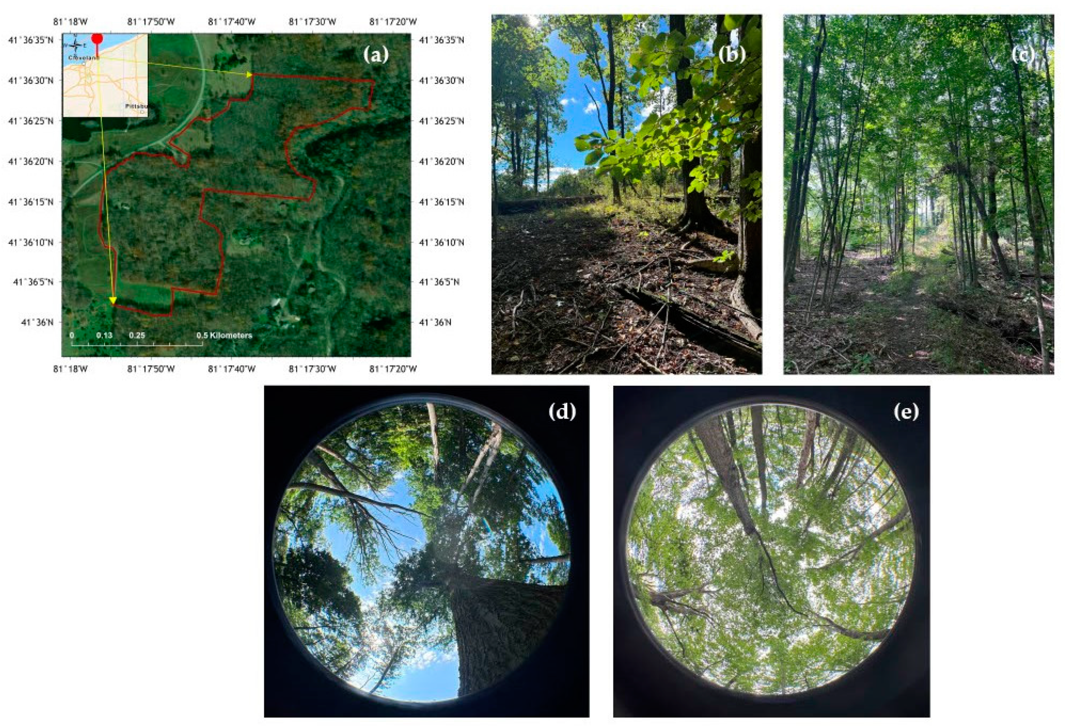
The study was conducted at the Working Woods in the Holden Arboretum, Kirtland, Ohio, United States (41.60163° N, 81.29797° W) (Figure 2), during the peak of the growing season from 31 May 2024 to 9 September 2024. The study area spans approximately 3 acres and is part of the 67 acres of the Working Woods Learning Forest at Holden Forests and Gardens. The forest canopy is dominated by Sugar Maple (Acer saccharum), Northern Red Oak (Quercus rubra), White Ash (Fraxinus americana), Hickory (Carya sp.), and American Beech (Fagus grandifolia), with canopy heights ranging approximately between 15 and 25 m. During the study period, the average precipitation and the average temperature were 61.9 mm and 21.6 °C, respectively [31]. The soil was classified as Sandy Loam to Loam (Hydrometer method).
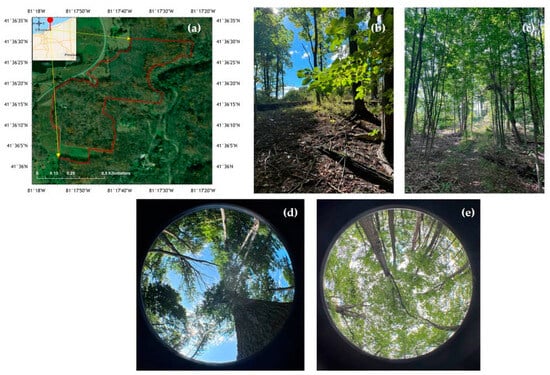
Figure 2.
Location of the study site where 38 plots were located. (a) Location map of the study area, (b) area subjected to edge feathering, (c) control site, and upward-facing hemispherical images of (d) edge feathering and (e) control site, respectively.
At the edge of the forest, an “edge feathering” treatment was implemented in Spring 2021. Edge feathering is a land-management technique in which a gradual transition is created between a forest edge and an adjacent land type, intending to increase wildlife habitat benefits such as increasing hiding places or food resources and biodiversity in plants, birds, and wildlife. This treatment involved felling trees along the edge of the forest-meadow line, ceasing regular mowing of the adjacent meadow, and planting native trees and shrubs in that adjacent field in a strip approximately 9–15 m wide. Instead of a sharp division between meadow and forest, this treatment created a gradual transition, with varying canopy densities from the forest interior to the edge. In contrast, control plots were left with the previously sharp division between meadow and forest, largely with an uninterrupted canopy, except for natural disturbances. The meadow adjacent to the forested area lacked any significant canopy cover. Along the feathered area, shrubs and young trees were planted in the meadow to provide a more gradual transition between the two ecosystem types. The edge-feathered forest was south-facing, so control plots without treatment were also selected from south-facing forest edges to control for the effect of edge orientation on light availability and species composition [10]. This directional consistency minimized any potential variation in light availability due to changes in sunlight direction over time. Treatment-specific characteristics are given in Table A1 [32].
2.2. Edge Feathering Design
Edge feathering was implemented along the perimeter of the selected forest edge. The primary objective of this technique was to create a gradual transition between the forest interior and the surrounding landscape. To achieve this, a non-uniform thinning and cutting approach was employed. While shade-tolerant species such as Beech and Maple were prioritized for removal, Oak trees, which require higher light levels, were retained to promote their vigor and reproductive potential. Edge feathering was conducted along approximately 120 m of the south-facing Woodline edge in 2021 in Holden Arboretum, Kirtland Ohio (Figure 2). The depth of the edge feathering cutting varied, reaching up to 30 m into the woods. Care was taken to avoid slopes and streams, and the depth of each zone was maintained within a range of 9–10 m. Variations in depth were introduced to create structural complexity within the edge. The creation of structurally complex edges was a key consideration in the feathering design. This involved creating openings of varying sizes and shapes, rather than uniform clearings.
2.3. Cutting Intensity and Tree Species Selection and Removal
Three zones of cutting intensity were established along the edge. The first zone, located immediately adjacent to the pre-existing woodline, involved the removal of approximately 75% of shade-tolerant trees. The second zone removed 50% of the canopy, while the third removed up to 25% (Figure 1). The selection of tree species for removal was based on their competitive proximity to healthier or better-formed trees, shade tolerance, and the overall desired forest structure. The practice of mowing the field between the forest edges was discontinued in 2021, followed by extensive planting of 22 different species of bare-root native shrubs and trees in this area along the wooded edge in Spring 2021. Cutting and removing trees were carried out with assistance from the Ohio Division of Wildlife and Division of Forestry.
2.4. Invasive Species Removal and Planting
Ongoing invasive woody understory removal was integral to the edge feathering process. Treatment has occurred annually since edge feathering was implemented to prevent invasive species from dominating as light levels change. Additionally, planting to enhance habitat diversity and promote native plant growth was implemented. Bare-root shrubs and trees were planted along the south-facing woodlines in 2021. In subsequent years, approximately 15% of the planted individuals were replanted to replace those that had died.
2.5. Plot Arrangement
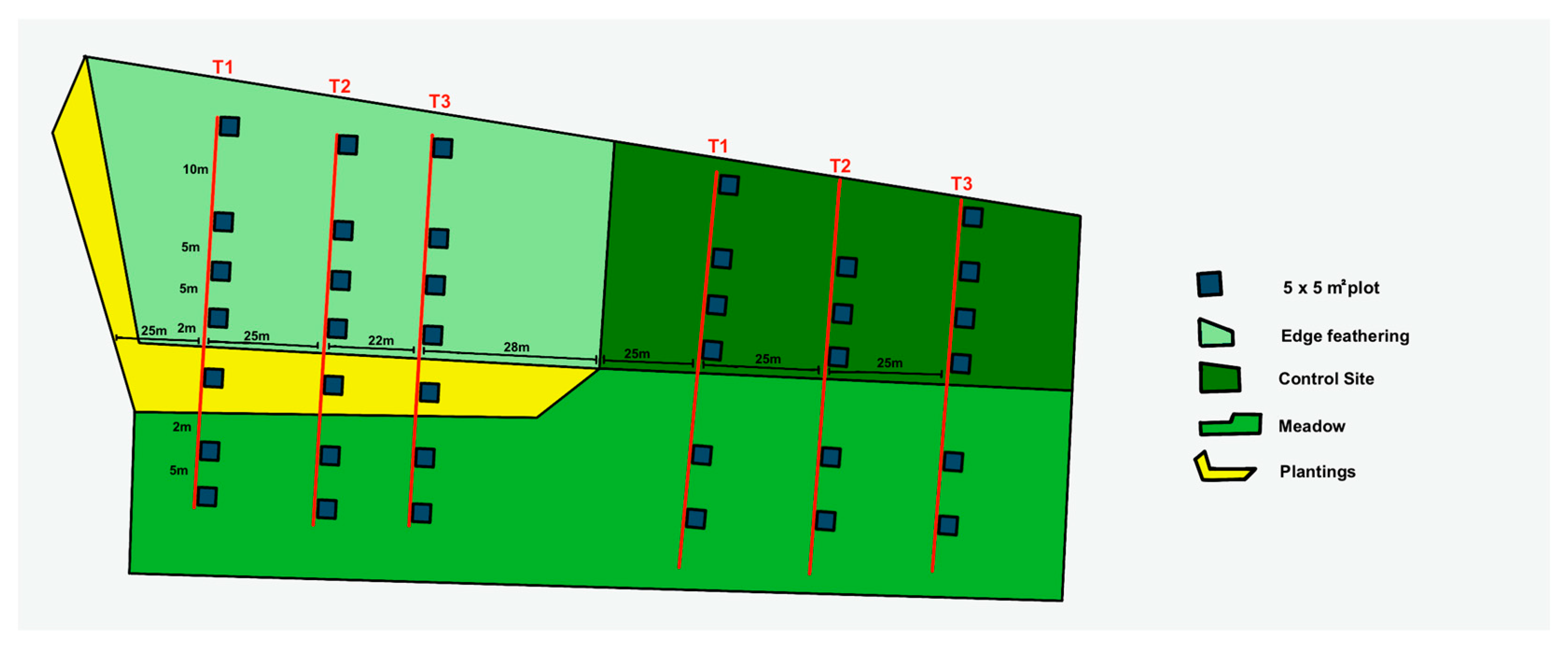
At each of the four treatments—edge feathering, control, meadow, and plantings—we systematically established 12 sampling plots, each measuring 5 m by 5 m, to assess vegetation composition. To minimize the disturbance from the nearby walking path and the respective neighboring treatment, we established transects 25 m away from the path and the treatment. In the edge-feathered treatment site, plots were placed along a canopy openness gradient (75%, 50%, 25%, and core forest with 0% clearing). These plots were arranged in a single transect, with one plot representing each gradient level, totaling four plots per transect. For the meadow planting site adjacent to the edge-feathering area, three additional plots were installed along with the established transects. Meadow transects were positioned directly in front of forest edges, with two plots in each transect extending towards the meadow’s interior and one plot in edge planting. For the control site, we mirrored the transect and plot arrangement used in the edge feathering site; however, due to construction constraints, one transect contained only three plots instead of four (Figure 3). Transects were generally spaced 25 m apart to minimize overlap and potential site-related biases. However, one transect in the edge-feathered site had to be placed closer to a neighboring transect (22 m apart) due to accessibility challenges [16].
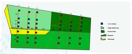
Figure 3.
Experimental Design for the Vegetation Composition Assessment. This diagram represents the experimental design across the study site, including treatments: edge feathering, control, meadow, and plantings. At each site, 38 sampling plots (5 m × 5 m each) were established and systematically arranged to minimize disturbance from nearby paths and neighboring treatments.
In selecting the plot locations, we took care to avoid potential confounding factors such as hiking trails, steep slopes, and streams, focusing instead on stands with gentle slopes [7]. Given the small size of some undisturbed areas within the study sites where proximity to hiking trails or managed forest areas posed challenges, additional plots were selected randomly by proceeding in a single direction from the previous plot. To prevent overlap and ensure distinct sampling areas, we maintained a minimum distance of 5 m between the edges of any two plots and a 10 m gap between adjacent plots within the treatment and core forest areas in the edge feathered site (Figure 3). These methodological considerations ensured that the sampling design was systematic and adaptable to the specific conditions of each study site.
2.6. Sampling of Understory Vegetation
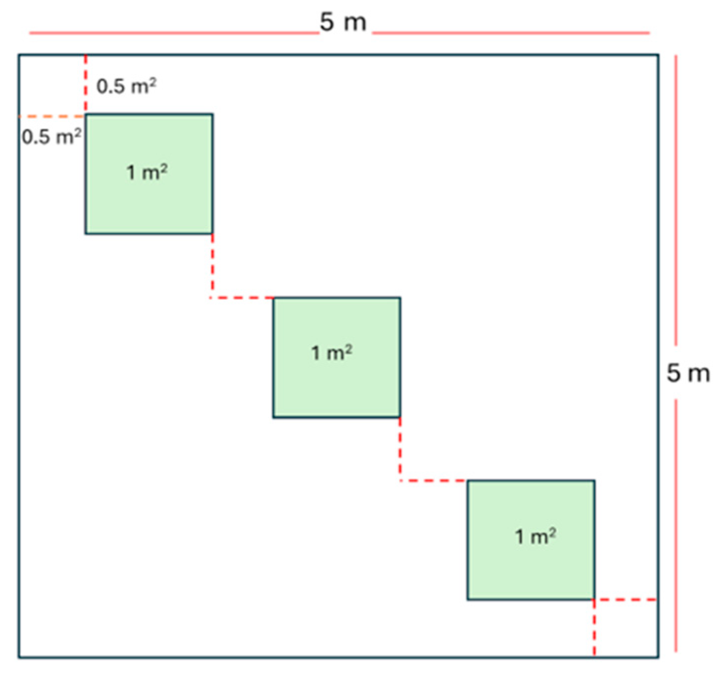
Vegetation sampling was conducted using the quadrant method by systematically placing quadrants (subplots hereafter) within the 5 m2 experimental plots. Each plot contained three designated subplots labeled A, B, and C, each measuring 1 m2 (Figure 4). This design resulted in 114 subplots across the study area, corresponding to 38 experimental plots (Figure 3).
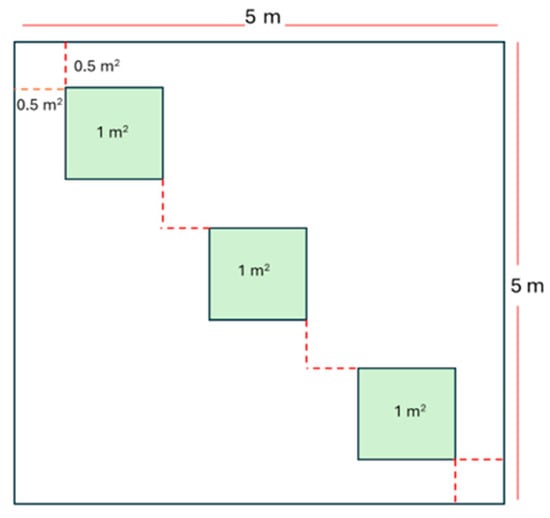
Figure 4.
Schematic diagram of sampling plot. At each plot, there are three subplots per plot and a setup along the line of symmetry.
The understory vegetation, covering all vascular plant species below 1.3 m in height (breast height), was monitored and recorded. Plant species were identified in the field using field guides; species that could not be identified on-site were photographed for later identification [33,34,35,36,37,38]. The number of individuals and their percent leaf cover were recorded for each species. Percent cover was estimated using a visual assessment method conducted by a single observer to minimize personal bias [39].
2.7. Light Measurements and Analysis
Light intensity and quality (R: FR ratio) were measured using a manual Photosynthetic Photon Flux Density (PPFD) meter (Spectrum Technologies, Inc., Aurora, IL, USA, Field Scout Quantum Meter, SN: 288) and a Red/ Far-red light meter (Spectrum Technologies, Inc., Aurora, IL, USA, Field Scout Quantum Meter, SN: 862), respectively. Measurements were conducted in each plot along three distinct sub-transects, with each sub-transect comprising five sampling points, resulting in a total of 15 data points per plot. Measurements were taken on sunny days between 10:30 a.m. and 2:00 p.m., a period when solar radiation is typically strongest and at a height of 1.3 m above ground level [40]. To ensure uniformity in light conditions, data collection was performed on days with clear weather, avoiding cloudy or rainy conditions. Additionally, measurements were taken in calm conditions, with no wind present, to minimize interference with readings.
2.8. Soil pH Analysis
Topsoil samples, each approximately 20 g, were collected to a depth of 10 cm from the organic layer at five predetermined points within each experimental plot in the study area, ensuring representative variations of the plots. The samples were transported to the laboratory and air-dried for 24 h to remove moisture and stabilize them for further analysis. Following the drying period, the pH of each sample was measured using a soil-water suspension prepared at a 1:2.5 ratio of soil to distilled water. pH measurements were conducted with an Accumet Basic pH Meter (Thermo Fisher Scientific Inc., Waltham, MA, USA), following the guidelines explained in the Standard operating procedure for soil pH Determination by the Food and Agriculture Organization of the United Nations. Prior to measurements, the pH meter was calibrated using standard buffer solutions to ensure the accuracy and reliability of the readings.
2.9. Statistical Analysis
2.9.1. Is There a Difference Between Mean and Heterogeneity in Light Intensity and Red-to-Far-Red Ratio Among Treatments?
To analyze the effect of treatment on light intensity, we employed a linear mixed-effects model (LMMs) using the lme4 package in R software version 4.2.2 (2022) [41]. The light intensity was modeled with treatment as a fixed effect and plot as the random effect to control for variability due to plot-level differences. Model assumptions were evaluated, but the bimodal distribution of light intensity could not be adequately normalized through transformation, resulting in some violations in assumptions. Model diagnostics were assessed with and without data transformation; however, since transformation did not improve the model fit, we proceeded with the non-transformed data. We tested the significance of the treatment effects using Anova (type II) in the car package [42]. Post hoc comparisons of treatment means were performed using the estimated marginal means with the emmeans package [43]. A similar method was applied to the R:FR ratio as well.
To calculate the heterogeneity of light intensity and the red-to-far-red ratio, the median values of each point along the sub-transects were taken. The coefficient of variation (CV) for light intensity and the red-to-far-red ratio were calculated for each canopy clearance at each plot in each treatment. To analyze the heterogeneity within each plot, we calculated the coefficient variation (CV) of measured variables (light quantity and light quality) based on the data from the 15 different points. The CV is defined as the ratio of the standard deviation to the mean, expressed as a percentage. To evaluate the homogeneity of variances among the different canopy clearances across treatments, Levene’s test was conducted to test the equality of light heterogeneity among the treatment levels. For CV that differed in heterogeneity across the treatments in Levene’s, a non-parametric Kruskal–Wallis test was performed to determine whether there were significant differences in the median among the treatment groups. Then, for the significant results via Kruskal–Wallis, we performed post hoc Dunn’s test to identify specific pairwise differences among the treatment groups.
2.9.2. Does Edge Feathering Influence Plant Community Diversity and Total Cover?
To assess plant species diversity, richness, evenness, and total cover, we analyzed the effect of the treatment as a predictor variable. We calculated these metrics using the vegan package in R, specifically estimating the Shannon Diversity Index, Simpson Index (D), Inverse Simpson Index ((1/D), also known as the Simpson Diversity Index), species richness, Pielou’s evenness index, and species cover based on field survey data. Linear mixed models (LMMs) were constructed with the lme4 package, applying the lmer function for diversity indices and Pielou’s evenness index. The plot was included as the random effect for most models; however, for Pielou’s evenness index, the subplot was used as the random effect to address singularity issues encountered when the plot was used. To model species richness data, we used generalized linear mixed-effect models (GLMMs) with the glmer.nb function from the lme4 package [13], employing a negative binomial distribution. Model residual diagnostics were performed using the DHARMa package to confirm assumptions were well met for all the models. Analysis of Variance (Anova) with Type II sum of squares was used to evaluate the effect of treatment on diversity parameters. Post hoc pairwise comparisons of treatment levels were conducted using the emmeans package. Data were log-transformed as necessary to meet model assumptions.
2.9.3. Is Light Heterogeneity a Better Predictor of Diversity and Richness than Mean Light Availability?
We used model selection to determine the best predictor(s) of species diversity in our data set. We used a Generalized Linear Model (GLM) to analyze the relationship between the species diversity-related response variables and the explanatory variables (light intensity and its heterogeneity). To identify the best model that explains the variability in diversity, we employed stepwise model selection using the Akaike Information Criterion (AIC). The stepAIC function from the MASS package was used to select the model in both forward and backward directions [44] and we present the model with the lowest AIC (Table A5). Non-transformed data were used for model selection and residual diagnostics were performed using the DHARMa package to confirm the assumptions.
2.9.4. Does a Greater Heterogeneity of Light Availability Correlate with Greater Plant Community Diversity?
We used the results from our model selection approach (research question 3, above) to inform our next analysis. To assess whether greater variation in light availability correlates with increased plant richness and diversity, we employed Generalized Linear Models (GLMs) using the glm function. The coefficient of variation (CV) of light intensity was used as the explanatory variable, while the diversity indices—Shannon Diversity Index, Inverse Simpson Index, Species Richness and Cover Proportion were used as response variables. For these continuous response variables, we selected a Gaussian family for the GLM. In contrast, for the cover proportion data, we used a quasi-binomial family to account for overdispersion. Model diagnostics were done, and model assumptions were well met. All analyses were conducted in R software version 4.2.2 (2022) [41].
3. Results
3.1. Is There a Difference Between Mean and Heterogeneity in Light Intensity and Red-to-Far-Red Ratio Among Management Treatments?
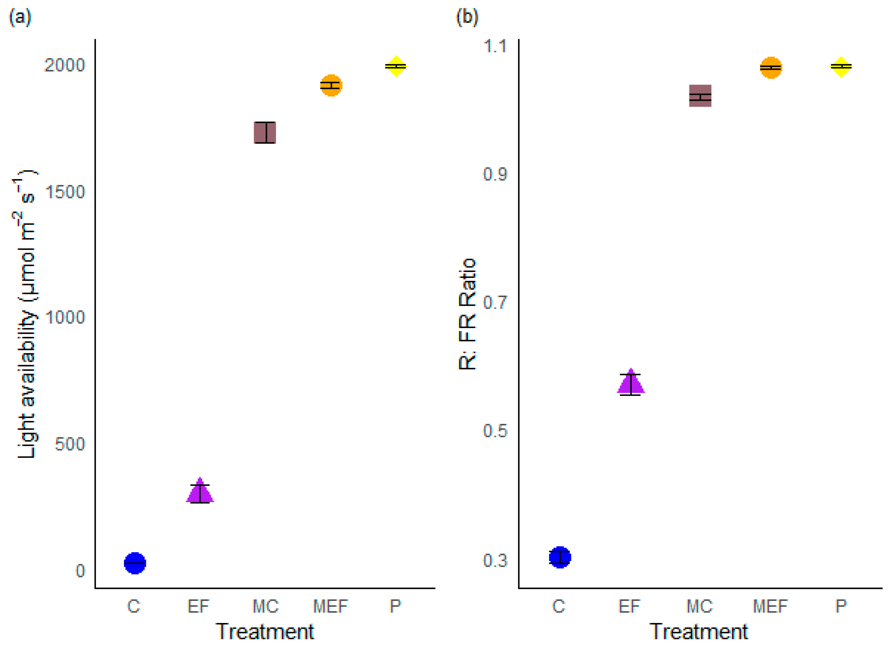
The treatments had a significant effect on both mean light intensity (χ2 = 3134.5, df = 4, p < 2.2 × 10⁻¹⁶) and mean R: FR ratio (χ2 = 2362.2, df = 4, p < 2.2 × 10⁻¹⁶) (Table 1). Mean light intensity and R:FR ratio were significantly higher in the edge feathered treatment than in the control treatment (Table A2). Mean light intensity was twelve times higher and R:FR ratio was 1.5 times higher in edge feathered treatment compared to control treatment. Meadow plots had a high overall mean in light availability compared to forest plots (Figure 5).

Table 1.
Anova table of the main effect of treatment on mean light availability.
Table 1.
Anova table of the main effect of treatment on mean light availability.
| Response Variable | Chisq | Df | p Value |
|---|---|---|---|
| Mean Light Intensity | 3134.5 | 4 | <2.2 × 10⁻¹⁶ *** |
| Mean R: FR ratio | 2362.2 | 4 | <2.2 × 10⁻¹⁶ *** |
Significant effects are indicated by asterisks next to the p-values. *** indicate p < 0.001.
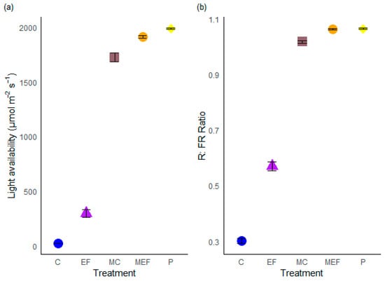
Figure 5.
The mean light availability (a) and mean red-to-far-red ratio (b) over five treatments. C (Control), EF (Edge Feathering), MC (Meadow opposite to Control site), MEF (Meadow opposite to edge feathered area), and P (Planting). Means (±SE) are presented. Each colored symbol represents a distinct treatment.
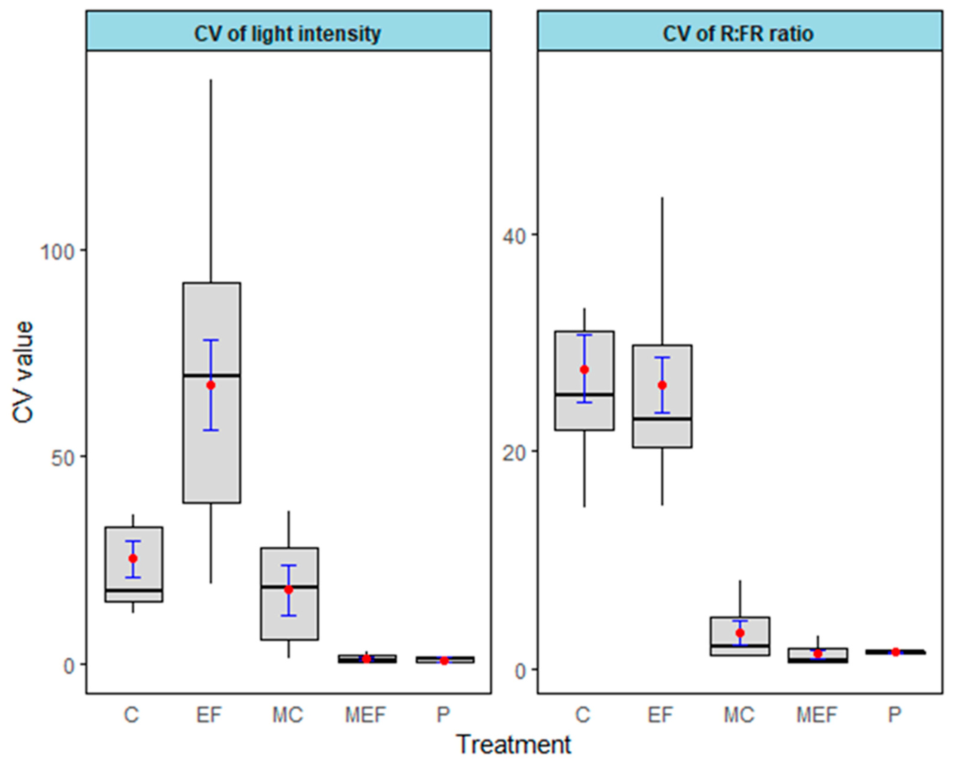
Edge feathering plots had a high overall heterogeneity in light intensity compared to the control. Edge feathering significantly influenced the heterogeneity of light intensity (Figure 6, Table 2). The open areas have very low heterogeneity (Figure 6). The Kruskal–Wallis test revealed a significant difference in median CV values across treatments for light intensity (χ2 = 25.785, df = 4, p = 3.497 × 10⁻⁵) and R:FR ratio (χ2 = 27.098, df = 4, p = 1.899 × 10⁻⁵) (Table 3). Dunn’s post hoc test was conducted to identify specific pairwise differences in median CV values for light intensity and R: FR ratio across different treatment groups. Treatment effects on the median variability of light intensity were marginally significant between control and edge feathering treatments (p = 0.0707). Median light heterogeneity also differed between the meadow and forest plots (Table A3).
Table 2.
Levene’s test results for homogeneity of variances of light availability across treatments.
Table 2.
Levene’s test results for homogeneity of variances of light availability across treatments.
| Response Variable | Df | F Value | p Value |
|---|---|---|---|
| CV of Light Intensity | 4, 33 | 7.5517 | 0.0001957 *** |
| CV of R: FR ratio | 4, 33 | 3.0909 | 0.02884 * |
Significant effects are indicated by asterisks next to the p-values. * indicates p < 0.05, and *** indicate p < 0.001.
Table 3.
Kruskal–Wallis rank sum test for differences in median light intensity CV across treatment groups.
Table 3.
Kruskal–Wallis rank sum test for differences in median light intensity CV across treatment groups.
| Response Variable | Chisq | Df | p Value |
|---|---|---|---|
| CV of Light Intensity | 25.785 | 4 | 3.497 × 10⁻⁵ |
| CV of R: FR ratio | 27.098 | 4 | 1.899 × 10⁻⁵ |
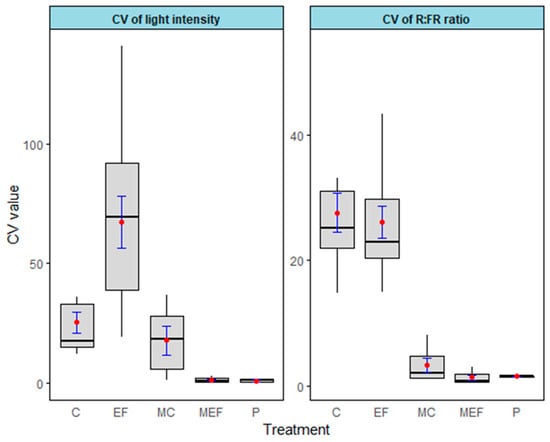
Figure 6.
The light heterogeneity (coefficient of variation) light intensity and red-to-far-red ratio over five treatments. C (Control), EF (Edge Feathering), MC (Meadow opposite to Control site), MEF (Meadow opposite to edge feathered area), and P (Planting). Error bars are in blue (±SE).
Figure 6.
The light heterogeneity (coefficient of variation) light intensity and red-to-far-red ratio over five treatments. C (Control), EF (Edge Feathering), MC (Meadow opposite to Control site), MEF (Meadow opposite to edge feathered area), and P (Planting). Error bars are in blue (±SE).
3.2. Does Edge Feathering Influence Plant Species Richness and Total Cover?
A total of 179 understory plant species were recorded in the study area. Among these, 153 species were identified at the species level, and 164 were identified at the genus level, representing 53 families and 104 genera. The family Asteraceae was the most abundant, comprising 23% of the 5691 understory plant individuals, followed by the Rosaceae and Poaceae families, respectively. In the edge feathering treatment, 75% of the recorded plant species were native, while 25% were non-native.
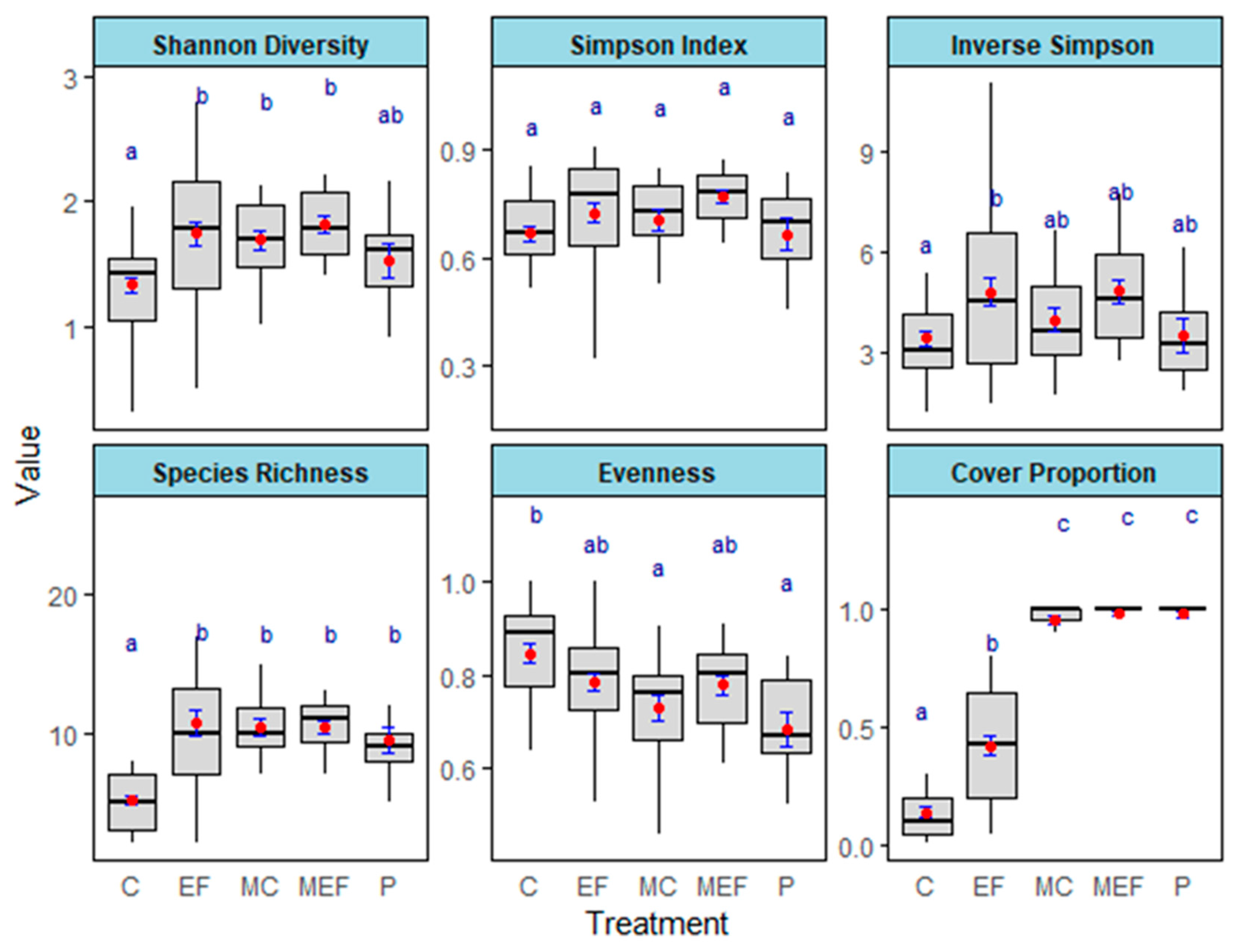
We found large differences in diversity across treatments for the Shannon index (χ2 = 25.265, df = 4, p = 4.45 × 10⁻⁵), Simpson’s diversity index (1/D) (χ2 = 13.885, df = 4, p = 0.007671), species richness (χ2 = 67.573, df = 4, p = 7.38 × 10⁻¹⁴), and Pielou’s evenness (χ2 = 22.35, df = 4, p = 0.0001707). However, the effect of treatment on the Simpson index (D) was marginally significant (χ2 = 8.7309, df = 4, p = 0.06819) (Figure 7, Table 4).
In every diversity index, except Pielou’s evenness, edge feathered plots showed a greater diversity compared to the unmanaged control plots (p < 0.05) (Table A4). Edge feathering increased species richness by more than twofold (p < 0.0001) and both Shannon’s and Simpson’s diversity indices by approximately 1.5-fold (p < 0.05) compared to the unmanaged control. Open meadow plots consistently exhibited significantly higher cover proportions compared to forested plots (p < 0.05) (Table A4).
Table 4.
Anova table of the main effect of treatment on understory plant diversity indices in LMMs.
Table 4.
Anova table of the main effect of treatment on understory plant diversity indices in LMMs.
| Response Variable | Chisq | Df | p-Value |
|---|---|---|---|
| Shannon index | 25.265 | 4 | 4.45 × 10⁻⁵ *** |
| Simpson index (D) | 8.7309 | 4 | 0.06819 |
| Simpson’s Diversity Index (1/D) | 13.885 | 4 | 0.007671 ** |
| Species richness | 67.573 | 4 | 7.38 × 10⁻¹⁴ *** |
| Pielou’s evenness | 22.35 | 4 | 0.0001707 *** |
| Total cover | 505.59 | 4 | 2.2 × 10⁻¹⁶ *** |
Significant effects are indicated by asterisks next to the p-values. ** indicate p < 0.01 and *** indicate p < 0.001.

Figure 7.
The effects of treatments on the diversity indices such as Shannon Diversity, Simpson Index, Inverse Simpson index, Species Richness, Evenness, and Cover Proportion after 3.5 years of edge feathering treatment (C—Control; EF—Edge Feathered; MEF—Meadow adjacent to edge-feathering site; MC—Meadow adjacent to the control site; and P: Plantings). Red points are the means (±SE) in blue. Means that share a lowercase blue letter are not significantly different.
3.3. Is Light Heterogeneity a Better Predictor of Diversity and Richness than Mean Light Availability?
The model that included CV in light intensity and CV in R: FR, was identified as the best model for both Shannon and Simpson Diversity Index (1/D) (Table 5), as it had the lowest AIC and deviance values (Table A5). Removing either of these predictors significantly worsened the model fit, resulting in much higher AIC values and highlighting the importance of both variables in explaining diversity. For species richness, evenness, and cover proportion, the best models included mean light availability in addition to CV of light intensity (Table 5). However, manually excluding mean light intensity did not change the slopes for CV of light intensity or CV of R: FR (pers. obs.). The best model for cover proportion also included the CV of pH as an additional predictor (Table 5). While the best models selected by AIC generally included CV of R: FR, separate models with just this predictor indicated that it was not significant on its own (p > 0.05) (except for cover proportion, also see Table A6). Therefore, we did not include this variable in question 3.4 below.
Table 5.
Diversity measures as a function of environmental variables. Summary of the best-performing models following model selection.
3.4. Does Greater Heterogeneity of Light Availability Correlate with Higher Plant Community Diversity?
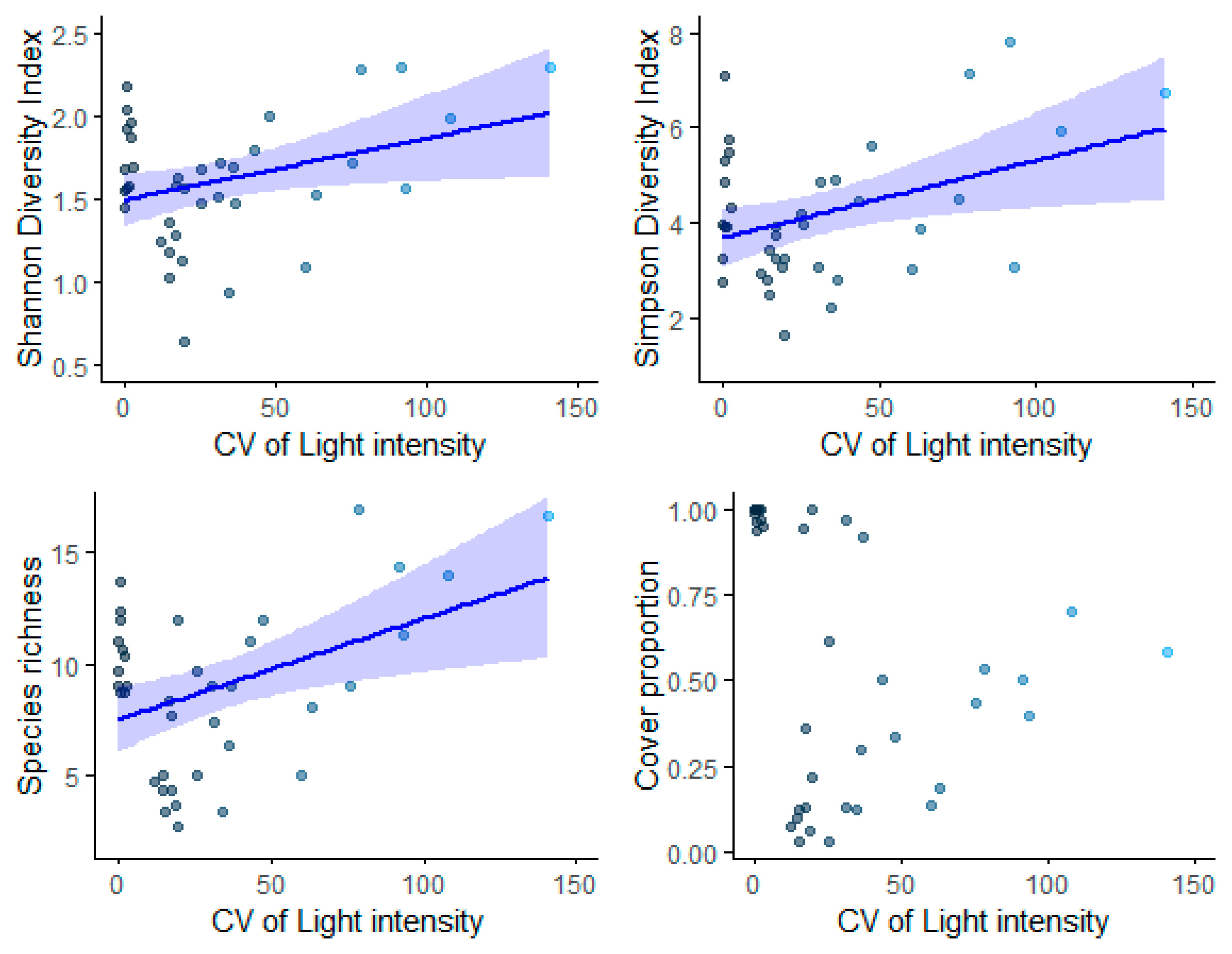
Plant community diversity assessed using Shannon Diversity (p = 0.0382), Simpson Diversity Index (1/D) (p = 0.0161), and species richness (p = 0.00801) exhibited a positive relationship with the coefficient of variation (CV) of light intensity (Table 6, Figure 8). However, there was no significant relationship between the CV of light intensity and species cover (Table 6, Figure 8).
Table 6.
Summary of generalized linear models examining the effects of light heterogeneity on understory plant species diversity indices.
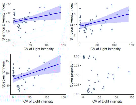
Figure 8.
The effect of heterogeneity of light (CV of light intensity) on species diversity metrics, including the Shannon Diversity Index, the Simpson Diversity Index (1/D), species richness, and cover proportion per 5 m2 in the forest understory. The ribbons indicate a 95% confidence interval of the regression.
4. Discussion
4.1. Edge Feathering Increased Mean Light Availability and Light Heterogeneity
Consistent with our hypothesis, edge feathering increased the availability and heterogeneity of light compared to the unmanaged control site. The twelvefold increase in mean light intensity and the 1.5-fold increase in the R: FR ratio suggest that edge feathering effectively reduces canopy cover, allowing greater penetration of light and a shift toward higher red-to-far-red ratios. These findings are consistent with previous studies that report increased light penetration following canopy thinning, as thinning reduces canopy density and allows more light to reach the understory [15,25,29,30,32]. Another study found that light intensities significantly increased in 25% and 50% canopy clearance of monocultural Cryptomeria japonica plantations in Taiwan immediately after canopy thinning [28]. Our study found that the heterogeneity in light intensity increased by more than 2.5-fold compared to the control, highlighting its effectiveness in significantly altering the light environment within ecotonal zones. This increase in heterogeneity reflects a key outcome of canopy modification, as it disrupts uniform light distribution and introduces variability critical for microenvironmental dynamics [13]. However, Yu et al. [29] argued that selective tree removal to reduce forest density results in a more uniform light distribution than unaltered forests by creating a more even canopy structure that minimizes light patchiness. In contrast, our findings indicate a different pattern, suggesting that canopy modifications can enhance, rather than homogenize, light variability. However, some studies found that while the effect of canopy thinning on overall light availability diminished after a decade, the variability in light availability remained twice as high as in the control, suggesting a legacy effect of canopy thinning on light heterogeneity [14]. This highlights the importance of considering temporal dynamics when evaluating the long-term effects of canopy modification treatments. Our study was completed only 3.5 years after thinning treatment, a snapshot in time of light levels that have been changing since the treatment. With more time, results would be different, indicating how disturbance within ecosystems can increase heterogeneity.
4.2. Edge Feathering Increased Plant Community Diversity
Our findings demonstrate that the edge feathering treatment significantly influenced plant diversity across multiple metrics, including Shannon Diversity, Simpson’s Diversity (1/D), and species richness, with all measures showing greater diversity in the edge feathered site compared to the control. The consistent trend across diversity indices underscores the positive impact of edge feathering on plant community structure. These results support our hypothesis that edge feathering treatment increases diversity, including species richness and total cover compared to unmanaged control plots.
Our results align with previous studies that report increased plant diversity in response to canopy thinning and other forest management practices that reduce competition and promote resource partitioning [6,23,32,45,46]. Moreover, the significant increase in species richness suggests that edge feathering can facilitate colonization by new species, possibly due to improved conditions for seed germination and establishment [23,46,47]. While we did not look at changes in species composition for this study, it is likely that with thinning, there was a shift towards more shade-intolerant species that contributed to the increases in species richness (pers. observations, e.g., Liriodendron tulipifera, Solidago bicolor, Symphyotrichum lanceolatum, and Potentilla simplex).
However, some studies showed that the effects of thinning treatments on understory vegetation can vary or even be negligible, depending on factors such as the specific vegetation layers considered and the time after thinning [7,29]. Some studies have shown that species richness significantly increases shortly after thinning [30,46]. For example, Cheng et al. [30] indicated that species richness peaked approximately half a year post-treatment before declining at two and a half years post-thinning. This temporal variation in species richness suggests that thinning can initially create favorable conditions for species colonization and establishment, which may diminish as the ecosystem begins to stabilize [14]. In comparison, our study found significant increases in plant diversity and richness in response to edge feathering after three and a half years, indicating that its effects on diversity metrics may persist longer or follow a different mechanism, potentially due to differences in treatment intensity and the structural variations of the ecotones. Replication across sites and time is needed to understand the role of context in shaping community responses to edge feathering.
Studies showed that thinning not only improves the light conditions but also leads to a faster decomposition rate of the remaining leaf and root litter. This is because the establishment of shrubs and herbs after thinning creates a more favorable environment for decomposer organisms [32,46]. In the edge feathering treatment here, felled tree residues were left on-site, potentially providing a greater nutrient contribution compared to sites where trees were removed. Other unmeasured environmental drivers, such as microbial community composition and interactions, may also influence the observed patterns and should be considered in future studies to gain a more complete understanding of edge feathering.
4.3. Light Heterogeneity Was the Best Predictor of Plant Species Diversity
Our results highlight the likely role of light heterogeneity in shaping plant community diversity and structure across the studied ecotones. These findings align with the heterogeneity-diversity hypothesis, which posits that greater environmental variability enhances species coexistence by increasing niche availability and reducing competitive exclusion [48]. These results highlight the importance of resource heterogeneity particularly light in shaping species diversity discussed in the heterogeneity-diversity hypothesis, as greater variability in light conditions likely creates a wider range of ecological niches, allowing more species to coexist [13,19,49]. Also, this aligns with previous findings that show heterogeneous light environments significantly drive understory plant richness [13].
However, previous studies on light availability and variability have yielded mixed conclusions, often emphasizing the context-dependent nature of these relationships [18,19,50], which may depend on spatial scale, differences in the mean, or unmeasured environmental variables. While previous studies have reported negative heterogeneity-diversity relationships at smaller spatial scales, where environmental variability can favor competitive dominance and reduce diversity [23,50], our study demonstrates a positive relationship between light heterogeneity and plant diversity, even at a relatively small scale. This challenges the assumption that heterogeneity at fine scales universally reduces diversity and highlights the context-dependent nature of these relationships [51]. It is, however, consistent with the argument that environmental filters might be more important than historical factors (such as dispersal) in driving local community composition [52]. This could also be due to the recent change—perhaps with more time since the treatment, even if heterogeneity remains, the plant communities could stabilize and some species increase in dominance. The reviews on this topic have also highlighted the importance of resource quantity in driving species diversity in young and mature stands, while resource heterogeneity often becomes more influential in old-growth stands. While resource quantity remains a consistent driver of diversity in both disturbed and undisturbed forests, in disturbed forests, resource heterogeneity plays a greater role due to the patchy distribution of resources caused by disturbances [15,19]. Our study adds to this body of evidence by showing that edge feathering—a practice that increases light heterogeneity—promotes increased plant diversity. Furthermore, some studies suggest that light heterogeneity alone may not influence species richness unless accompanied by soil heterogeneity [13,19]. Here, we measured the heterogeneity of soil pH and generally found it to be a weaker predictor of plant community diversity, though additional measures in the soil are needed to rule soil heterogeneity out as an important driver of diversity in this system.
5. Conclusions
Edge feathering increased light heterogeneity, correlating with higher plant richness and diversity in temperate deciduous forest-meadow ecotones. These improvements likely enhance wildlife habitat quality by boosting food resources and structural complexity [11]. Critically, our simultaneous measurement of vegetation and light availability, accounting for seasonal and short-term variability, strengthens causal links between management practices and ecological outcomes. The legacy effect of canopy thinning on light dynamics [14] further supports edge feathering as a durable intervention, even as direct light effects diminish over time. To our knowledge, this analysis represents the first assessment of responses of temperate deciduous forest-meadow ecotone to edge feathering land management practice. Understanding how edge feathering land management practice shapes the dynamics of forest-meadow boundaries represents a step toward predicting the future applicability of this technique.
Author Contributions
Conceptualization, R.M.S. and J.M.M.; methodology, R.M.S., J.M.M., A.D.K., and J.H.B.; formal analysis, A.D.K.; resources, J.H.B.; data curation, A.D.K.; writing—original draft preparation, A.D.K.; writing—review and editing, A.D.K., J.H.B., J.M.M., and R.M.S.; supervision, J.H.B.; project administration, J.M.M. All authors have read and agreed to the published version of the manuscript.
Funding
This research received no external funding.
Data Availability Statement
Data are archived in the Open Science Framework. 10.17605/OSF.IO/TYJB4.
Acknowledgments
We thank the National Science Foundation (DEB 2217714 to JHB) for funding. We also thank The Holden Arboretum in Kirtland, Ohio, for providing the research site. We thank Nathan Gilbert, Annabel Degenholtz, and Jessica Furlough for their help with data collection and Benjamin Gorham in the Digital Scholarship team at Kelvin Smith Library, Case Western Reserve University, for assisting preparation of the map for the study site.
Conflicts of Interest
The authors declare no conflicts of interest.
Abbreviations
The following abbreviations are used in this manuscript:
EF—Edge Feathering Site; C—Control Site; P—Planting Site; MEF—Meadow opposite to Edge Feathering Site; and MC—Meadow opposite to Control site
Appendix A
Table A1.
Main characteristics of experimental sites.
Table A1.
Main characteristics of experimental sites.
| Descriptives | EF | Control | Meadow-Opposite to EF Site | Meadow-Opposite to Control Site | Planting |
|---|---|---|---|---|---|
| ID | EF | C | MEF | MC | P |
| Geographical Coordinates | 41.60156° N −81.29818° W | 41.60156° N −81.29616° W | 41.60098° N −81.29803° W | 41.600888° N, −81.296374° W | 41.601337° N, −81.298155° W |
| Landscape type | Managed Forest | Core Forest | Meadow | Meadow | Managed Plantings |
| Soil moisture content (saturated) | 26.67% | 27.01% | 40.61% | 44.52% | 47.4% |
| Management | Selective tree removal and canopy opening at different intensities in 2021 | No specific management type | No specific management type | No specific management type | Planting of hardwood trees in 2021 |
| Size | ~0.88 acres (~3566.16 m2) | ~0.75 acres (~3048 m2) | ~0.49 acres (1989 m2) | ~0.42 acres (~1700 m2) | ~0.5 acres (2023 m2) |
| Mean Annual Temperature (°C) during Growth Period, 2021–2024 | 20.7 °C | ||||
| Mean annual precipitation during Growth Period, 2021–2024 | 99.55 mm | ||||
| Soil Type | Sandy Loam | Loam | Sandy Loam | Sandy Loam | Sandy Loam |
| Main overstory tree species (>20 cm DBH) | As, Qr, Fa | As, Qr, Ta | No overstory trees | Scattered As trees | No overstory trees |
| Number of plots (5 m2) | 12 | 11 | 6 | 6 | 3 |
| Number of subplots (1 m2) | 36 | 33 | 18 | 18 | 9 |
| Mean light availability (May–Early September) | 480.95 µmol m−2 s−1 | 32.39 µmol m−2 s−1 | 1912.07 µmol m−2 s−1 | 1729.27 µmol m−2 s−1 | 1984.08 µmol m−2 s−1 |
As—Acer saccharum; Qr—Quercus rubra; Fa—Fraxinus americana; Ta—Tilia americana.
Table A2.
Estimated marginal means and pairwise comparisons of mean light availability across treatment levels.
Table A2.
Estimated marginal means and pairwise comparisons of mean light availability across treatment levels.
| Treatment | Contrast | Estimate | SE | df | t Ratio | p Value |
|---|---|---|---|---|---|---|
| Mean Light intensity | C-EF | −285.3 | 32.3 | 563 | −8.82 | <0.0001 |
| C-MC | −1662.6 | 41.9 | 561 | −39.65 | <0.0001 | |
| C-MEF | −1850.6 | 41.9 | 561 | −44.135 | <0.0001 | |
| C-P | −1870.6 | 54.8 | 561 | −34.12 | <0.0001 | |
| EF-MC | −1377.3 | 41.9 | 556 | −32.834 | <0.0001 | |
| EF-MEF | −1565.4 | 41.9 | 556 | −37.318 | <0.0001 | |
| EF-P | −1585.3 | 54.8 | 559 | −28.91 | <0.0001 | |
| MC-MEF | −188.1 | 44.6 | 562 | −4.219 | 0.0003 | |
| MC-P | −208 | 56.9 | 565 | −3.657 | 0.0026 | |
| MEF-P | −19.9 | 56.9 | 565 | −0.35 | 0.9968 | |
| Mean R:FR ratio | C-EF | −0.27554 | 0.0148 | 562 | −18.675 | <0.0001 |
| C-MC | −0.72034 | 0.0191 | 565 | −37.683 | <0.0001 | |
| C-MEF | −0.76507 | 0.0191 | 565 | −40.024 | <0.0001 | |
| C-P | −0.7697 | 0.025 | 565 | −30.801 | <0.0001 | |
| EF-MC | −0.4448 | 0.0191 | 564 | −23.263 | <0.0001 | |
| EF-MEF | −0.48953 | 0.0191 | 564 | −25.603 | <0.0001 | |
| EF-P | −0.49416 | 0.025 | 564 | −19.772 | <0.0001 | |
| MC-MEF | −0.04473 | 0.0203 | 562 | −2.2 | 0.1813 | |
| MC-P | −0.04936 | 0.0259 | 564 | −1.903 | 0.3167 | |
| MEF-P | −0.00463 | 0.0259 | 564 | −0.179 | 0.9998 |
C indicates the control forest patch; EF indicates the edge-feathered forest patch; MEF indicates the open meadow area next to the edge-feathering site; MC indicates the open meadow area adjacent to the control site; and P indicates the planting area adjoining the edge-feathering area.
Table A3.
A post hoc Dunn test for Differences in Median Light Intensity CV across Treatment Groups.
Table A3.
A post hoc Dunn test for Differences in Median Light Intensity CV across Treatment Groups.
| Treatment | Contrast | Test Statistics | p Value |
|---|---|---|---|
| CV of Light intensity | C-EF | −2.26399 | 0.0707 |
| C-MC | 0.502466 | 0.6153 | |
| C-MEF | 2.482773 | 0.0521 | |
| EF-MC | 2.400105 | 0.0574 | |
| EF-MEF | 4.410193 | 0.0001 * | |
| MC-MEF | 1.740787 | 0.1634 | |
| P-C | 2.026683 | 0.1067 | |
| P-EF | 3.509077 | 0.0020 * | |
| P-MC | 1.506203 | 0.198 | |
| P-MEF | 0.084856 | 0.4662 | |
| CV of R:FR ratio | C-EF | 0.300492 | 0.7638 |
| C-MC | 3.143083 | 0.0067 * | |
| C-MEF | 3.911393 | 0.0005 * | |
| C-P | 2.633274 | 0.0254 | |
| EF-MC | 2.939485 | 0.0115 * | |
| EF-MEF | 3.719349 | 0.0009 * | |
| EF-P | 2.462786 | 0.0345 | |
| MC-MEF | 0.675381 | 0.9989 | |
| MC-P | 0.169675 | 0.4326 | |
| MEF-P | −0.38177 | 1 |
* C indicates the control forest patch; EF indicates the edge-feathered forest patch; MEF indicates the open meadow area next to the edge-feathering site; MC indicates the open meadow area adjacent to the control site; and P indicates the planting area adjoining the edge-feathering area.
Table A4.
Estimated marginal means and pairwise comparisons of diversity indices across treatment levels.
Table A4.
Estimated marginal means and pairwise comparisons of diversity indices across treatment levels.
| Treatment | Contrast | Estimate | SE | df | t Ratio | p Value |
|---|---|---|---|---|---|---|
| Shannon Index | C-EF | −0.4324 | 0.0985 | 106 | −4.388 | 0.0003 |
| C-MC | −0.3573 | 0.128 | 109 | −2.792 | 0.0477 | |
| C-MEF | −0.4854 | 0.128 | 109 | −3.793 | 0.0022 | |
| C-P | −0.2215 | 0.1675 | 109 | −1.322 | 0.6782 | |
| EF-MC | 0.0751 | 0.1281 | 109 | 0.586 | 0.9768 | |
| EF-MEF | −0.053 | 0.1281 | 109 | −0.414 | 0.9938 | |
| EF-P | 0.2109 | 0.1676 | 109 | 1.258 | 0.717 | |
| MC-MEF | −0.1281 | 0.1358 | 106 | −0.943 | 0.8794 | |
| MC-P | 0.1358 | 0.1736 | 108 | 0.782 | 0.9352 | |
| MEF-P | 0.2639 | 0.1736 | 108 | 1.52 | 0.5518 | |
| Simpson Index (D) | C-EF | −0.0599 | 0.0318 | 106.9 | −1.884 | 0.3321 |
| C-MC | −0.0401 | 0.0411 | 99.5 | −0.977 | 0.8651 | |
| C-MEF | −0.1043 | 0.0411 | 99.5 | −2.54 | 0.09 | |
| C-P | −0.003 | 0.0552 | 88.1 | −0.054 | 1 | |
| EF-MC | 0.0198 | 0.041 | 93 | 0.482 | 0.9888 | |
| EF-MEF | −0.0445 | 0.041 | 93 | −1.084 | 0.8142 | |
| EF-P | 0.0569 | 0.0551 | 83.6 | 1.031 | 0.8401 | |
| MC-MEF | −0.0642 | 0.0438 | 106.2 | −1.465 | 0.5871 | |
| MC-P | 0.0371 | 0.0573 | 106.2 | 0.648 | 0.9667 | |
| MEF-P | 0.1013 | 0.0573 | 106.2 | 1.769 | 0.397 | |
| Simpson Diversity Index (1/D) | C-EF | −1.4063 | 0.433 | 107 | −3.25 | 0.0131 |
| C-MC | −0.5854 | 0.562 | 108 | −1.041 | 0.8356 | |
| C-MEF | −1.4359 | 0.562 | 108 | −2.554 | 0.0866 | |
| C-P | −0.2929 | 0.74 | 107 | −0.396 | 0.9947 | |
| EF-MC | 0.8209 | 0.562 | 105 | 1.459 | 0.5909 | |
| EF-MEF | −0.0296 | 0.562 | 105 | −0.053 | 1 | |
| EF-P | 1.1134 | 0.74 | 105 | 1.505 | 0.5617 | |
| MC-MEF | −0.8506 | 0.596 | 106 | −1.426 | 0.6123 | |
| MC-P | 0.2925 | 0.766 | 109 | 0.382 | 0.9954 | |
| MEF-P | 1.1431 | 0.766 | 109 | 1.492 | 0.5697 | |
| Species richness | C-EF | −0.76936 | 0.0962 | Inf | −7.996 | <0.0001 |
| C-MC | −0.66824 | 0.1172 | Inf | −5.703 | <0.0001 | |
| C-MEF | −0.67356 | 0.1171 | Inf | −5.754 | <0.0001 | |
| C-P | −0.57403 | 0.1496 | Inf | −3.836 | 0.0012 | |
| EF-MC | 0.10112 | 0.1026 | Inf | 0.986 | 0.8618 | |
| EF-MEF | 0.09579 | 0.1024 | Inf | 0.935 | 0.8833 | |
| EF-P | 0.19532 | 0.1386 | Inf | 1.41 | 0.6214 | |
| MC-MEF | −0.00533 | 0.1096 | Inf | −0.049 | 1 | |
| MC-P | 0.0942 | 0.1437 | Inf | 0.656 | 0.9657 | |
| MEF-P | 0.09953 | 0.1437 | Inf | 0.693 | 0.9581 | |
| Pielou’s evenness | C-EF | 0.06133 | 0.0268 | 107 | 2.287 | 0.1572 |
| C-MC | 0.11818 | 0.0326 | 107 | 3.624 | 0.004 | |
| C-MEF | 0.06829 | 0.0326 | 107 | 2.094 | 0.2302 | |
| C-P | 0.16333 | 0.0418 | 107 | 3.903 | 0.0015 | |
| EF-MC | 0.05685 | 0.0321 | 107 | 1.77 | 0.3967 | |
| EF-MEF | 0.00695 | 0.0321 | 107 | 0.216 | 0.9995 | |
| EF-P | 0.102 | 0.0415 | 107 | 2.459 | 0.1079 | |
| MC-MEF | −0.04989 | 0.0371 | 107 | −1.345 | 0.6638 | |
| MC-P | 0.04515 | 0.0454 | 107 | 0.994 | 0.8576 | |
| MEF-P | 0.09504 | 0.0454 | 107 | 2.092 | 0.2311 | |
| Cover proportion | C-EF | −0.29068 | 0.0352 | 106 | −8.268 | <0.0001 |
| C-MC | −0.79848 | 0.0456 | 109 | −17.495 | <0.0001 | |
| C-MEF | −0.82404 | 0.0456 | 109 | −18.055 | <0.0001 | |
| C-P | −0.81603 | 0.0597 | 109 | −13.664 | <0.0001 | |
| EF-MC | −0.5078 | 0.0457 | 109 | −11.12 | <0.0001 | |
| EF-MEF | −0.53336 | 0.0457 | 109 | −11.679 | <0.0001 | |
| EF-P | −0.52535 | 0.0597 | 109 | −8.794 | <0.0001 | |
| MC-MEF | −0.02556 | 0.0485 | 106 | −0.527 | 0.9844 | |
| MC-P | −0.01755 | 0.0619 | 108 | −0.284 | 0.9986 | |
| MEF-P | 0.00801 | 0.0619 | 108 | 0.129 | 0.9999 |
C indicates the control forest patch; EF indicates the edge-feathered forest patch; MEF indicates the open meadow area next to the edge-feathering site; MC indicates the open meadow area adjacent to the control site; and P indicates the planting area adjoining the edge-feathering area.
Table A5.
Summary of all performed model selections to test the hypothesis.
Table A5.
Summary of all performed model selections to test the hypothesis.
| Response Variable | Best Model | Distribution | Model Type | Null Deviance | Residual Deviance |
|---|---|---|---|---|---|
| Shannon_Diversity | Shannon_Diversity~Light_intensity_CV + CV_RFR_ratio | Normal | glm | 5.3433 | 3.1232 |
| Inverse_Simpson | Inverse_Simpson~Light_intensity_CV + CV_RFR_ratio | Normal | glm | 78.75 | 55.48 |
| Species_richness | Species_richness~Light_intensity_CV + CV_RFR_ratio + Mean_Light_intensity | Normal | glm | 511.2 | 168.3 |
| Evenness | Evenness~Light_intensity_CV + Mean_Light_intensity | Normal | glm | 0.2732 | 0.1822 |
| Cover_prop | Cover_prop~Light_intensity_CV + Mean_Light_intensity + CV_pH | Quasi-poisson | glm | 5.246 | 0.5065 |
The full model is Response variable~Light_intensity_CV + CV_RFR_ratio + Mean_Light_intensity + Mean_R_FR + CV_pH. Light_intensity_CV represents the coefficient of variation of light intensity, CV_RFR_ratio indicates the coefficient of variation of the red-to-far-red (R:FR) ratio, Mean_Light_intensity represents the mean intensity of photosynthetically active radiation, Mean_R_FR represents the mean value of the R: FR ratio, and CV_pH represents the coefficient of variation of pH values.
Table A6.
Summary of generalized linear models examining the effects of heterogeneity of R:FR on understory plant species diversity indices.
Table A6.
Summary of generalized linear models examining the effects of heterogeneity of R:FR on understory plant species diversity indices.
| Diversity Matrix | Predictor | Estimate | Std. Error | t Value | p Value |
|---|---|---|---|---|---|
| Shannon Diversity | CV of R:FR | −0.006006 | 0.004330 | −1.387 | 0.174 |
| Simpson Diversity Index (1/D) | CV of R:FR | −0.005636 | 0.017034 | −0.331 | 0.743 |
| Species richness | CV of R:FR | −0.06889 | 0.04192 | −1.643 | 0.109 |
| Cover proportion | CV of R:FR | −0.021084 | 0.002653 | −7.947 | 1.96 × 10⁻⁹ |
References
- Peyras, M.; Vespa, N.I.; Bellocq, M.I.; Zurita, G.A. Quantifying Edge Effects: The Role of Habitat Contrast and Species Specialization. J. Insect Conserv. 2013, 17, 807–820. [Google Scholar] [CrossRef]
- Esin, M.N.; Ruchin, A.B. Ruchin. Edge Effects on Diptera Distribution in Deciduous Forests of the Centre of European Russia. J. Wildl. Biodivers. 2024, 8, 16–37. [Google Scholar] [CrossRef]
- Magura, T.; Lövei, G.L. The Permeability of Natural versus Anthropogenic Forest Edges Modulates the Abundance of Ground Beetles of Different Dispersal Power and Habitat Affinity. Diversity 2020, 12, 320. [Google Scholar] [CrossRef]
- Haugo, R.D.; Halpern, C.B.; Bakker, J.D. Landscape Context and Long-Term Tree Influences Shape the Dynamics of Forest-Meadow Ecotones in Mountain Ecosystems. Ecosphere 2011, 2, art91. [Google Scholar] [CrossRef]
- Kark, S. Effects of Ecotones on Biodiversity. In Encyclopedia of Biodiversity; Elsevier: Amsterdam, The Netherlands, 2013; pp. 142–148. [Google Scholar] [CrossRef]
- Ares, A.; Neill, A.R.; Puettmann, K.J. Understory Abundance, Species Diversity and Functional Attribute Response to Thinning in Coniferous Stands. For. Ecol. Manag. 2010, 260, 1104–1113. [Google Scholar] [CrossRef]
- Taki, H.; Inoue, T.; Tanaka, H.; Makihara, H.; Sueyoshi, M.; Isono, M.; Okabe, K. Responses of Community Structure, Diversity, and Abundance of Understory Plants and Insect Assemblages to Thinning in Plantations. For. Ecol. Manag. 2010, 259, 607–613. [Google Scholar] [CrossRef]
- Wuyts, K.; De Schrijver, A.; Vermeiren, F.; Verheyen, K. Gradual Forest Edges Can Mitigate Edge Effects on Throughfall Deposition If Their Size and Shape Are Well Considered. For. Ecol. Manag. 2009, 257, 679–687. [Google Scholar] [CrossRef]
- Matlack, G.R. Microenvironment Variation within and among Forest Edge Sites in the Eastern United States. Biol. Conserv. 1993, 66, 185–194. [Google Scholar] [CrossRef]
- De Pauw, K.; Sanczuk, P.; Meeussen, C.; Depauw, L.; De Lombaerde, E.; Govaert, S.; Vanneste, T.; Brunet, J.; Cousins, S.A.O.; Gasperini, C.; et al. Forest Understorey Communities Respond Strongly to Light in Interaction with Forest Structure, but Not to Microclimate Warming. New Phytol. 2022, 233, 219–235. [Google Scholar] [CrossRef]
- Edgefeathering.Pdf. Available online: https://fw.ky.gov/wildlife/documents/edgefeathering.pdf (accessed on 23 September 2024).
- Barbier, S.; Gosselin, F.; Balandier, P. Influence of Tree Species on Understory Vegetation Diversity and Mechanisms Involved—A Critical Review for Temperate and Boreal Forests. For. Ecol. Manag. 2008, 254, 1–15. [Google Scholar] [CrossRef]
- Helbach, J.; Frey, J.; Messier, C.; Mörsdorf, M.; Scherer-Lorenzen, M. Light Heterogeneity Affects Understory Plant Species Richness in Temperate Forests Supporting the Heterogeneity-Diversity Hypothesis. Ecol. Evol. 2022, 12, e8534. [Google Scholar] [CrossRef] [PubMed]
- Tsai, H.-C.; Chiang, J.-M.; McEwan, R.W.; Lin, T.-C. Decadal Effects of Thinning on Understory Light Environments and Plant Community Structure in a Subtropical Forest. Ecosphere 2018, 9, e02464. [Google Scholar] [CrossRef]
- Su, X.; Wang, M.; Huang, Z.; Fu, S.; Chen, H.Y.H. Forest Understorey Vegetation: Colonization and the Availability and Heterogeneity of Resources. Forests 2019, 10, 944. [Google Scholar] [CrossRef]
- Bartemucci, P.; Messier, C.; Canham, C.D. Overstory Influences on Light Attenuation Patterns and Understory Plant Community Diversity and Composition in Southern Boreal Forests of Quebec. Can. J. For. Res. 2006, 36, 2065–2079. [Google Scholar] [CrossRef]
- Beck, J.J.; Givnish, T.J. Fine-Scale Environmental Heterogeneity and Spatial Niche Partitioning among Spring-Flowering Forest Herbs. Am. J. Bot. 2021, 108, 63–73. [Google Scholar] [CrossRef] [PubMed]
- Dormann, C.F.; Bagnara, M.; Boch, S.; Hinderling, J.; Janeiro-Otero, A.; Schäfer, D.; Schall, P.; Hartig, F. Plant Species Richness Increases with Light Availability, but Not Variability, in Temperate Forests Understorey. BMC Ecol. 2020, 20, 43. [Google Scholar] [CrossRef]
- Bartels, S.F.; Chen, H.Y.H. Is Understory Plant Species Diversity Driven by Resource Quantity or Resource Heterogeneity? Ecology 2010, 91, 1931–1938. [Google Scholar] [CrossRef] [PubMed]
- Tamme, R.; Hiiesalu, I.; Laanisto, L.; Szava-Kovats, R.; Pärtel, M. Environmental Heterogeneity, Species Diversity and Co-Existence at Different Spatial Scales. J. Veg. Sci. 2010, 21, 796–801. [Google Scholar] [CrossRef]
- Zhang, H.; Jiao, X.; Zha, T.; Lv, X.; Ni, Y.; Zhang, Q.; Wang, J.; Ma, L. Developmental Dynamics and Driving Factors of Understory Vegetation: A Case Study of Three Typical Plantations in the Loess Plateau of China. Forests 2023, 14, 2353. [Google Scholar] [CrossRef]
- Smith, E. Ecological Relationships Between Overstory and Understory Vegetation in Ponderosa Pine Forests of the SouthwestKaibab Natl. For. 2011, 16. Available online: https://www.fs.usda.gov/Internet/FSE_DOCUMENTS/stelprdb5361521.pdf (accessed on 13 October 2024).
- Kern, C.C.; Montgomery, R.A.; Reich, P.B.; Strong, T.F. Harvest-Created Canopy Gaps Increase Species and Functional Trait Diversity of the Forest Ground-Layer Community. For. Sci. 2014, 60, 335–344. [Google Scholar] [CrossRef]
- Yang, H.; Pan, C.; Wu, Y.; Qing, S.; Wang, Z.; Wang, D. Response of Understory Plant Species Richness and Tree Regeneration to Thinning in Pinus Tabuliformis Plantations in Northern China. For. Ecosyst. 2023, 10, 100105. [Google Scholar] [CrossRef]
- Thomas, S.C.; Halpern, C.B.; Falk, D.A.; Liguori, D.A.; Austin, K.A. Plant diversity in managed forests: Understory responses to thinning and fertilization. Ecol. Appl. 1999, 9, 864–879. [Google Scholar] [CrossRef]
- Anderson, M.C. Light relations of terrestrial plant communities and their measurement. Biol. Rev. 1964, 39, 425–481. [Google Scholar] [CrossRef]
- Augspurger, C.K.; Salk, C.F. Understory Plants Evade Shading in a Temperate Deciduous Forest amid Climate Variability by Shifting Phenology in Synchrony with Canopy Trees. PLoS ONE 2024, 19, e0306023. [Google Scholar] [CrossRef]
- Chiang, J.-M.; Lin, K.-C.; Hwong, J.-L.; Wang, H.-C.; Lin, T.-C. Immediate Effects of Thinning with a Small Patch Clearcut on Understory Light Environments in a Cryptomeria Japonica Plantation in Central Taiwan. Taiwan J. For. Sci. 2012, 27, 319–331. [Google Scholar]
- Yu, J.; Zhang, X.; Xu, C.; Hao, M.; Choe, C.; He, H. Thinning Can Increase Shrub Diversity and Decrease Herb Diversity by Regulating Light and Soil Environments. Front. Plant Sci. 2022, 13, 948648. [Google Scholar] [CrossRef]
- Cheng, C.; Wang, Y.; Fu, X.; Xu, M.; Dai, X.; Wang, H. Thinning Effect on Understory Community and Photosynthetic Characteristics in a Subtropical Pinus Massoniana Plantation. Can. J. For. Res. 2017, 47, 1104–1115. [Google Scholar] [CrossRef]
- US Department of Commerce, N. Climate. Available online: https://www.weather.gov/wrh/climate (accessed on 10 December 2024).
- Dang, P.; Gao, Y.; Liu, J.; Yu, S.; Zhao, Z. Effects of Thinning Intensity on Understory Vegetation and Soil Microbial Communities of a Mature Chinese Pine Plantation in the Loess Plateau. Sci. Total Environ. 2018, 630, 171–180. [Google Scholar] [CrossRef] [PubMed]
- Newcomb, L. Newcomb’s Wildflower Guide, 2011th ed.; Little, Brown and Company: New York, NY, USA, 1977. [Google Scholar]
- Undersander, D.; Casler, M.; Cosgrove, D.; Martin, N.E. Identifying Pasture Grasses; University of Wisconsin—Extension: Madison, WI, USA, 1996. [Google Scholar]
- Little, E.L. National Audubon Society Field Guide to North American Trees Eastern Region, 25th ed.; Alfred A. Knopf, Inc.: New York, NY, USA, 2006. [Google Scholar]
- Gleason, H.A.; Cronquist, A. Manual of Vascular Plants of Northeastern United States and Adjacent Canada; New York Botanical Garden: Bronx, NY, USA, 1991. [Google Scholar]
- Braun, E.L.; Weishaupt, C.G. The Monocotyledoneae: Cat-Tails to Orchids; Ohio State University Press: Columbus, OH, USA, 1967. [Google Scholar]
- Holmgren, N.H. Illustrated Companion to Gleason and Cronquist’s Manual: Illustrations of the Vascular Plants of Northeastern United States and Adjacent Canada; New York Botanical Garden: Bronx, NY, USA, 1998. [Google Scholar]
- Bråkenhielm, S.; Qinghong, L. Comparison of Field Methods in Vegetation Monitoring. In Biogeochemical Monitoring in Small Catchments; Černý, J., Novák, M., Pačes, T., Wieder, R.K., Eds.; Springer: Dordrecht, The Netherlands, 1995; pp. 75–87. [Google Scholar] [CrossRef]
- Prévost, M.; Raymond, P. Effect of Gap Size, Aspect and Slope on Available Light and Soil Temperature after Patch-Selection Cutting in Yellow Birch–Conifer Stands, Quebec, Canada. For. Ecol. Manag. 2012, 274, 210–221. [Google Scholar] [CrossRef]
- Bates, D.; Maechler, M.; Bolker, B.; Walker, S. Lme4: Linear Mixed-Effects Models Using “Eigen” and S4, 2003, 1.1-35.5. Available online: https://cran.r-project.org/web/packages/lme4/index.html (accessed on 24 October 2024).
- Fox, J.; Weisberg, S.; Price, B. Car: Companion to Applied Regression, 2001, 3.1-3. Available online: https://cran.r-project.org/web/packages/car/index.html (accessed on 28 October 2024).
- Lenth, R.V. Emmeans: Estimated Marginal Means, Aka Least-Squares Means, 2017, 1.10.5. Available online: https://cran.r-project.org/web/packages/emmeans/index.html (accessed on 30 October 2024).
- Ripley, B.; Venables, B. MASS: Support Functions and Datasets for Venables and Ripley’s MASS, 2009, 7.3-61. Available online: https://cran.r-project.org/web/packages/MASS/index.html (accessed on 30 October 2024).
- Bekris, Y.; Prevéy, J.S.; Brodie, L.C.; Harrington, C.A. Effects of Variable-Density Thinning on Non-Native Understory Plants in Coniferous Forests of the Pacific Northwest. For. Ecol. Manag. 2021, 502, 119699. [Google Scholar] [CrossRef]
- Xu, X.; Wang, X.; Hu, Y.; Wang, P.; Saeed, S.; Sun, Y. Short-Term Effects of Thinning on the Development and Communities of Understory Vegetation of Chinese Fir Plantations in Southeastern China. PeerJ 2020, 8, e8536. [Google Scholar] [CrossRef] [PubMed]
- Richardson, P.J.; MacDougall, A.S.; Larson, D.W. Fine-scale Spatial Heterogeneity and Incoming Seed Diversity Additively Determine Plant Establishment. J. Ecol. 2012, 100, 939–949. [Google Scholar] [CrossRef]
- Melbourne, B.A.; Cornell, H.V.; Davies, K.F.; Dugaw, C.J.; Elmendorf, S.; Freestone, A.L.; Hall, R.J.; Harrison, S.; Hastings, A.; Holland, M.; et al. Invasion in a Heterogeneous World: Resistance, Coexistence or Hostile Takeover? Ecol. Lett. 2007, 10, 77–94. [Google Scholar] [CrossRef] [PubMed]
- Ricklefs, R.E. Environmental Heterogeneity and Plant Species Diversity: A Hypothesis. Am. Nat. 1977, 111, 376–381. [Google Scholar] [CrossRef]
- Su, X.; Zheng, G.; Chen, H.Y.H. Understory Diversity Are Driven by Resource Availability Rather than Resource Heterogeneity in Subtropical Forests. For. Ecol. Manag. 2022, 503, 119781. [Google Scholar] [CrossRef]
- Davies, K.F.; Chesson, P.; Harrison, S.; Inouye, B.D.; Melbourne, B.A.; Rice, K.J. Spatial heterogeneity explains the scale dependence of the native–exotic diversity relationship. Ecology 2005, 86, 1602–1610. [Google Scholar] [CrossRef]
- Jiménez-Alfaro, B.; Girardello, M.; Chytrý, M.; Svenning, J.-C.; Willner, W.; Gégout, J.-C.; Agrillo, E.; Campos, J.A.; Jandt, U.; Kącki, Z.; et al. History and Environment Shape Species Pools and Community Diversity in European Beech Forests. Nat. Ecol. Evol. 2018, 2, 483–490. [Google Scholar] [CrossRef] [PubMed]
Disclaimer/Publisher’s Note: The statements, opinions and data contained in all publications are solely those of the individual author(s) and contributor(s) and not of MDPI and/or the editor(s). MDPI and/or the editor(s) disclaim responsibility for any injury to people or property resulting from any ideas, methods, instructions or products referred to in the content. |
© 2025 by the authors. Licensee MDPI, Basel, Switzerland. This article is an open access article distributed under the terms and conditions of the Creative Commons Attribution (CC BY) license (https://creativecommons.org/licenses/by/4.0/).