Abstract
This study examines the provision of ecosystem services in natural mixed broadleaf forests located in the Hyrcanian region of Iran. These services include habitat conservation, soil preservation, timber production, and carbon storage (C-stock). The forests are managed under three different silvicultural methods: shelterwood, selection cutting, and protection, allowing for a comparative analysis of their impact on these critical services. The time since the last cutting operation varied among the forest stands. In the shelterwood stand, 25 years had passed since the previous operation, while in the selection cutting stand, it had been 13 years. In contrast, the protected stand had remained untouched by logging for the past 40 years. This presents a valuable opportunity to assess the effects of the recovery period and evaluate the extent of ecosystem service restoration. Additionally, it allows for determining whether these services have reached the levels observed in a protected forest. The results show that habitat conservation, soil preservation, and carbon stock (C-stock) values ranked as follows: protection > selection cutting > shelterwood. In contrast, timber production values were highest under selection cutting, followed by shelterwood, and lowest in protected areas. Furthermore, the Stand Structural Complexity Index (SCI) was greatest in protected stands, with selection cutting and shelterwood-managed stands ranking second and third, respectively. Similarly, species diversity indices, the abundance of large-diameter trees, and the volume of deadwood followed this same trend. These findings highlight a trade-off in forest management practices. While selection cutting and shelterwood management simplify stand structure to enhance timber production and maximize economic returns, they also lead to a significant reduction in other critical forest ecosystem services. Our findings further revealed that, even decades after the cessation of forest operations, the ecological value of previously managed forests remains substantially lower than that of protected forests. Moreover, the results demonstrate that a single silvicultural rotation period is insufficient to fully restore the ecological value of managed forests, regardless of whether they were subjected to selection cutting or shelterwood management practices.
1. Introduction
Forest ecosystems provide a diverse range of ecosystem services (ES) that benefit communities at local, regional, and global scales [1,2,3]. These services encompass climate regulation, water supply, timber production, energy resources, biodiversity habitat, air purification, and erosion control, among others [4,5,6]. In recent decades, the concept and study of ecosystem services has garnered significant attention, particularly in the context of forest ecosystems [7,8,9].
The capacity of forests to provide these ecosystem services is influenced by a number of factors, such as stand type, species composition [10], stand age [11], silvicultural practices [12], and harvesting methods [13,14]. Additionally, natural disturbances (e.g., wildfires, drought, and insect infestations) and global environmental changes such as climate change, all have an effect on forest service potential [15].
As global demand for forest ecosystem services rises, balancing this demand with the impact of natural and anthropogenic pressures poses substantial challenges for forest managers and policymakers [5,16]. Intensive demand for forest resources has put significant stress on forest ecosystems, impacting their health and capacity to supply ES sustainably [17]. Therefore, understanding the mechanisms that influence ES provision is essential for informed forest management and effective policy-making [8]. Understanding the time required for forests to restore their ecosystem services (ES) after a disturbance is critically important. This can be achieved by comparing the levels of ecosystem services between managed forests and protected forests, providing valuable insights into the recovery process. Conducting this type of research poses significant challenges. In temperate ecosystems, the interval between consecutive silvicultural entries in managed forests is typically around a decade [18]. As a result, it is uncommon to find managed forests where the last silvicultural intervention occurred more than 10–15 years ago, making it difficult to evaluate the recovery period from a long-term perspective.
In the Hyrcanian forests of Iran, shelterwood management with a silvicultural rotation period of 20 to 25 years was practiced until 1990. From 1990 to 2017, selective cutting management with a 10-year rotation period was implemented. Since 2017, all logging operations in these forests have been prohibited, a ban that remains in effect to this day. Therefore, it is possible to quantify the changes and recovery of the forest ecosystem as a result of silvicultural interventions by comparing it with the control parcel, which usually has similar habitat conditions and stand structure to other parcels in the relevant series. The key questions guiding this research were: First, to what extent do silvicultural interventions impact ecosystem services in the Hyrcanian forests? And second, are the changes in forest services resulting from management interventions restored after a full silvicultural rotation period? Building on this context, the main objectives of this study were twofold: (a) to evaluate the effects of three forest management methods—shelterwood, selection cutting, and protection—on ecosystem services in mixed beech mountain forests in northern Iran, and (b) to assess the recovery process following the cessation of management activities. Specifically, we hypothesized that: (i) despite several years having passed since the last harvesting operation, natural forest stands managed for conservation purposes would exhibit higher biodiversity, improved soil conservation indicators, and greater carbon storage compared to previously managed stands; (ii) shelterwood management would optimize stem quality; and (iii) single-selection management would be less ecologically disruptive than shelterwood methods in terms of ecosystem services [18].
2. Materials and Methods
2.1. Study Area
This study was conducted in the Hyrcanian forests of Iran (Figure 1), a region covering 1.8 million hectares with high environmental, ecological, and economic value. These forests stretch from the southern shores of the Caspian Sea to elevations up to 2700 m above sea level on the northern slopes of the Alborz mountain range. They are characterized by a heterogeneous structure and diverse tree species, notably beech, which constitutes the largest area and volume of standing timber.
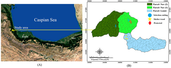
Figure 1.
Hyrcanian forest (A) and location of studied stands (B).
The study area is located in the Nav-Asalem forest, at coordinates 37°38′ N and 48°48′ E, with elevations between 700 and 1200 m above sea level (Table 1). Annual precipitation averages 963 mm, and the mean annual temperature is 8.8 °C. Historically, shelterwood management was practiced until 1990, after which it transitioned to selection cutting, which continued until 2017—the year a logging ban was implemented. Tree harvesting was conducted using chainsaws, and timber extraction relied on ground-based skidders equipped with winches. In the common shelterwood cutting system in the Hyrcanian forests of Iran, the various treatments consist of preparatory cutting (an optional initial treatment to increase tree vigor and seed production within a mature stand), regeneration cutting (a treatment to establish regeneration throughout the stand area) and light felling carried out before final cutting. The main objectives of shelterwood cutting are to develop seed trees by natural regeneration and encourage desirable species to achieve their maximum diameter growth. In forest management, the shelterwood cutting system involves a series of partial harvests conducted over several years, ultimately resulting in the establishment of a new even-aged stand. However, due to its negative impacts on silvicultural properties, biological diversity, and aesthetic values, shelterwood cutting has been largely replaced by selection cutting in these hardwood forests. In most Hyrcanian forests, a single-tree selection system has been adopted as a close-to-nature management approach, with interventions occurring every 10 years. This method aims to maintain uneven-aged tree populations, mimicking natural gap dynamics processes. The primary goal of selection-cutting management is to create mixed and uneven-aged stands that closely resemble natural forest ecosystems.

Table 1.
Study area characteristics in the different silvicultural managed stands (Sh: shelterwood cutting, Sc: selection cutting, Pr: protected).
This study evaluated three forest management approaches: shelterwood, selection cutting, and protection, the latter serving as a control. For this purpose, similar stands in terms of plant community and soil type and almost adjacent were selected (Figure 1). The selected stands all had an uneven-aged structure and the dominant stand type of fagetum mixed with other broadleaves. The number of stands selected in shelterwood cutting, selection cutting, and protected management was 3, 5, and 4 stands, respectively. The area of each stand varied from 15 to 20 hectares. The choice of these experimental blocks was made through a design-based approach, which is a statistical approach that establishes the methods of choice and use of the sites, allowing possible pseudoreplication problems to be overcome [19].
Table 1 provides additional details on the harvesting intensity and historical management practices within the study area.
2.2. Sampling Design and Data Collection
This study assessed the impact of three silvicultural methods (shelterwood, selection cutting, and protection) on four ecosystem service components: habitat conservation, soil conservation, timber production, and carbon storage. Habitat conservation was evaluated using indices of stand structural complexity (SCI), species diversity of trees, shrubs, and herbaceous plants, frequency of large-diameter trees (LDT), and volume of deadwood (standing and fallen). Soil conservation was assessed through soil physical and chemical properties under different management practices. Timber production was quantified by measuring the standing timber volume and calculating its economic value, while carbon storage was estimated for both trees and soil.
Sampling followed a systematic plot design with random starting points. Data on tree and stand structure, as well as soil properties, were collected using a 100 × 100-m grid. Circular sample plots with a radius of 17.85 m (1000 m2 in area) were established in each forest management type. Each parcel had between 45 and 55 plots, with a sampling intensity of approximately 9% (Table 2). Within each plot, three subplots (5 × 5 m) and one quadrat (1 × 1 m) were systematically positioned to assess vegetation characteristics across tree, shrub, and herb layers.
Table 2.
Area, number of plots, and sampling intensity in each silvicultural method (Sh: shelterwood cutting; Sc: selection cutting; Pr: protected).
Tree diameters (≥7.5 cm at breast height) and heights were measured within plots, with tree volume estimated using species-specific volume tables. Large-diameter trees (LDT), defined as those with a diameter ≥60 cm, were recorded separately. Deadwood (DW) volume was calculated using Huber’s formula, with both standing and fallen deadwood measured within the plots. Canopy cover was estimated as the proportion of sample points covered by the forest canopy. Species richness, cover, and abundance were recorded for each layer.
2.3. Measurement of Ecosystem Services
The species diversity of trees and understory, and the stand structural complexity index (SCI) were calculated by Equations (1)–(10).
Tree size diversity index (TDD)
The tree diameter diversity was obtained by Equation (1) [20]:
where n is number of diameter classes, Pi is proportion of individual tree in ith diameter class.
Tree height diversity index (THD)
The tree height diversity was obtained by Equation (2) [20]:
where n is number of height classes, Pi is proportion of individual tree in ith height class.
Canopy tree species richness index (TSRC)
The canopy tree species richness was obtained by Equation (3) [21]:
where n is number of species in canopy layer, Pi is proportion of basal area of ith species.
Tree species diversity index (TSD)
The tree species diversity was obtained by Equation (4) [22].
where TSD is tree species diversity index according to Shannon-Wiener index (H’), Pi is the ratio of the number of the ith species to the overall number of species.
Tree species evenness index (TSE)
The tree species evenness was obtained by Equation (5) [23].
where TSE is tree species evenness index according to the Pielou’s evenness index (Jsw), Pi is the ratio of the number of the ith species to the overall number of species, and S is the number of species.
Tree species richness index of trees (TSR), shrubs (ShSR), and herbs (HSR)
The tree species richness was obtained by Equation (6) [24].
where SR is species richness index according to the Margalef richness index (R’), S is the number of species, N is the total number of individuals of all species.
Stand structural complexity index (SCI)
The stand structural complexity index was obtained by Equation (7) [25,26].
where SCI is stand structural complexity index, TDD is tree diameter diversity, THD is tree height diversity, TSRC is species richness of canopy layer, ShSR is species richness of shrub layer, HSR is species richness of herb layer, and n refers to the number of structural attributes used in the index (n = 5).
The economic value of tree boles was estimated based on their species and quality as described in Table 3. The quality of standing tree boles was graded visually assessment based on the guidelines of the Iranian Natural Resources and Watershed Management Organization [27] and the quality of the first 6 m of tree boles with a diameter at breast height of larger than 42.5 cm was as follows: Q1: smooth, sound, cylindrical, circular cross-section, no rot, no twisting, no thick branches, suitable for veneering; Q2: sound, no rot, non-cylindrical or non-circular cross-section, with twisting, with one thick branch; Q3: with some rot, with a number of thick branches, with twisting; Fuel wood: heavily rotted, heavily twisted, with a lot of thick branches.
Table 3.
The economic value of tree boles (USD m−3).
To assess soil characteristics, two soil samples were collected from each plot: one from the center of the plot and the other randomly from the center of one of the quarter plots. Samples were taken from the upper 10 cm of soil using a steel cylinder with an inner diameter of 5 cm and a height of 10 cm.
The bulk density of the soil, which is the ratio of the dry weight of the soil to the volume of the soil sample (after drying the soil in the oven for 24 h at 105 °C), was calculated by Equation (8) [28].
In Equation (8), BD is bulk density in g cm−3, WD is dry weight of soil in g, and VC is volume of cylinder of soil sample in cm3.
The total soil porosity was determined using the Equation (9) [28].
In Equation (9), TP is the total porosity of the soil in percent, BD is the soil bulk density in g cm−3, and 2.65 is the density of soil particles (g cm−3) measured by a pycnometer on the same soil samples used to determine the bulk density.
The following characteristics were also determined: soil moisture content, using the weight method; soil organic carbon (OC) using the Walkley and Black method [29]; soil total nitrogen (N) using the Kjeldahl method [30]. The depth of litter was measured using a metal ruler to an accuracy of 1 mm. The C-stock of soil was determined using the Equation (10) [30].
where SCS is the soil carbon stock (Mg ha−1), BD is the soil bulk density (g cm−3), OC is the soil organic carbon (%), and e is the soil depth (m).
Allometric models were used to estimate the branch and leaf biomass of beech and hornbeam trees, as detailed in Table 4 [31]. Since the studied forests primarily consisted of pure or mixed beech stands, with beech accounting for over 85% of the total tree population, the bole, branch, and leaf biomass of other species was also estimated using allometric models developed for beech. Root biomass for all tree species was calculated as 20% of the total tree biomass. Carbon storage in tree components was determined by multiplying the biomass of each component by a conversion factor of 0.531 [32].
Table 4.
Allometric models to estimate biomass of beech tree components.
2.4. Data Analysis
Data were analyzed using SPSS software (version 22). The effects of forest management types on ecosystem service indicators were tested using ANOVA, with post-hoc comparisons made using Duncan’s test (α = 0.05). Data normality was assessed with the Kolmogorov-Smirnov test, and variance homogeneity was evaluated using Levene’s test (α = 0.05).
3. Results
3.1. Habitat Conservation
In all forest stands, tree canopy cover exceeded 76%, with the highest canopy cover observed in the protected (Pr) stands and the lowest in the shelterwood (Sh) stands (Table 5). Shrub canopy cover was highest in Pr stands, followed by selection cutting (Sc) and Sh stands, respectively. Similarly, herb cover was significantly greater in Pr stands than in Sc and Sh stands.
Table 5.
Stand attributes in each silvicultural method (Sh: shelterwood cutting; Sc: selection cutting; Pr: protected). Different letters in each row indicate a significant difference at α = 0.05 by Duncan’s test.
The frequency of trees, average diameter at breast height (DBH), basal area, and standing volume were significantly higher in Pr stands than in Sc and Sh stands. Tree height was comparable between Pr and Sc stands, both of which had greater tree heights than Sh stands.
The values for tree diameter diversity (TDD) and tree height diversity (THD) indices ranked Pr > Sc > Sh (Table 6). Additionally, species richness indices for the tree canopy, shrub, and herb layers were all highest in Pr stands, followed by Sc and Sh stands. The frequency and volume of both standing and fallen deadwood were also highest in Pr stands, with intermediate values in Sc stands and the lowest values in Sh stands. The frequency and volume of large-diameter trees (LDT) followed the same pattern. The Stand Structural Complexity Index (SCI) was highest in Pr stands (1.97), followed by Sc (1.47) and Sh stands (1.08) (Figure 2).
Table 6.
Stand structural diversity indicators in each silvicultural method (Sh: shelterwood cutting; Sc: selection cutting; Pr: protected). Acronyms: DW—deadwood; LDT—large diameter trees. Different letters in each row indicate a significant difference at α = 0.05 by Duncan’s test.
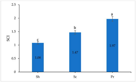
Figure 2.
Stand structural complexity index (SCI) in different silvicultural methods (Sh: shelterwood cutting; Sc: selection cutting; Pr: protected). Different letters (a, b and c) indicate significant differences at α = 0.05 by Duncan’s test.
3.2. Soil Conservation
Soil bulk density was highest in Sh stands, followed by Sc and Pr stands, while soil porosity was greatest in Pr stands (Table 7). Soil moisture content was significantly higher in Pr stands compared to Sh stands, with Sh stands exhibiting the lowest soil moisture levels. Soil organic carbon (OC) and total nitrogen (N) were also highest in Pr stands, with significantly higher values than in Sc and Sh stands. The C/N ratio in Pr stands was significantly higher than in the other stands, and litter depth was greatest in Pr stands, followed by Sc and Sh.
Table 7.
Soil properties in different silvicultural methods (Sh: shelterwood cutting; Sc: selection cutting; Pr: protected). Different letters in each row indicate a significant difference at α = 0.05 by Duncan’s test.
3.3. Timber Production and Economic Value
The volume and economic value of high-quality timber (Q1) were highest in Sc stands (171.19 m3/ha; USD 77,889.6/ha), followed by Pr and Sh stands (Table 8, Figure 3 and Figure 4). Timber quality Q1 ranked in the order Sc > Pr > Sh. For Q2 quality timber, Pr stands had the highest volume and economic value, with Sc and Sh stands exhibiting similar, lower levels. For Q3 quality timber, Pr and Sh stands had comparable volumes and values, both of which exceeded those in Sc stands. The volume and economic value of fuelwood followed the order Pr > Sc > Sh. Total woody volume, including timber and fuelwood, was highest in Pr stands, while total woody value ranked Pr = Sc > Sh.
Table 8.
Timber volume and value in different silvicultural managed stands (Sh: shelterwood cutting; Sc: selection cutting; Pr: protected). Different letters in each row indicate a significant difference at α = 0.05 by Duncan’s test.
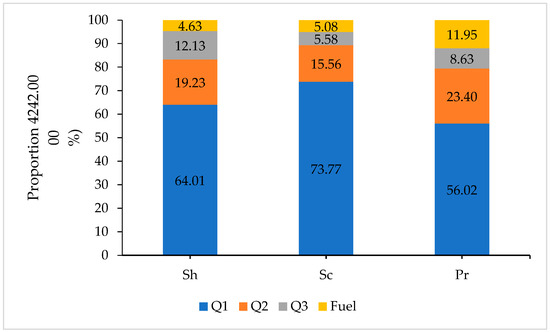
Figure 3.
Proportion (%) of timber volume in different silvicultural methods (Sh: shelterwood cutting; Sc: selection cutting; Pr: protected).
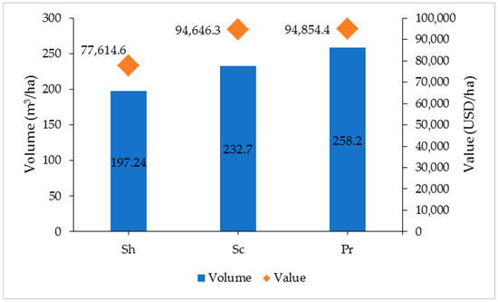
Figure 4.
Volume and value of timber in different silvicultural methods (Sh: shelterwood cutting; Sc: selection cutting; Pr: protected).
3.4. Carbon Stock
Carbon storage (C-stock) in tree components (bole, branches, crown, and roots) was significantly lower in Sh stands compared to Sc and Pr stands (Table 9). Whole-tree C-stock was also highest in Pr stands, followed by Sc and Sh (Figure 5). Soil C-stock was highest in protected stands (54.66 Mg ha−1), significantly greater than in Sc and Sh stands (Figure 6).
Table 9.
Carbon stock (Mean ± SD, Mg ha−1) in different silvicultural methods (Sh: shelterwood cutting; Sc: selection cutting; Pr: protected). Different letters in each row indicate a significant difference at α = 0.05 by Duncan’s test.
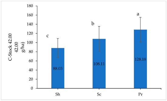
Figure 5.
C-stock in whole tree in different silvicultural methods (Sh: shelterwood cutting; Sc: selection cutting; Pr: protected). Different letters (a, b and c) indicate significant differences at α = 0.05 by Duncan’s test.
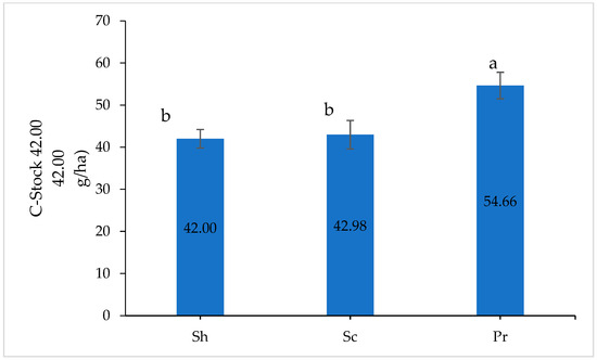
Figure 6.
C-stock in soil in different silvicultural methods (Sh: shelterwood cutting; Sc: selection cutting; Pr: protected). Different lowercase letters indicate significant difference at α = 0.05 by Duncan’s test.
4. Discussion
The first research hypothesis—that natural forest stands managed for conservation purposes exhibit higher biodiversity, improved soil conservation indicators, and greater carbon storage than previously managed stands, even several years after the last harvesting operation—was fully confirmed. This finding aligns with broader research indicating that preserving high-carbon-priority forests not only maintains significant carbon stocks but also supports greater species richness and structural diversity, contributing to enhanced ecosystem resilience. Previous studies have emphasized that the relationship between the absence of management and increased biodiversity is more complex than initially anticipated. The meta-analysis by Paillet et al. [33] revealed that species richness of tree species is generally higher in managed stands than in protected forests. These findings were confirmed by Schulze [34] concerning European beech temperate forests. Our research revealed that nearly all indicators of ecosystem health, including vegetation and soil parameters, were significantly better in protected areas compared to previously managed forests. A possible reason for the differences found comparing our results with European beech forests can be attributed to the higher biodiversity in the canopy layer which characterizes Hyrcanian forests. The higher level of species admixture in Iranian hardwood stands likely contributes to a more complex ecosystem, which is inherently more sensitive to external disturbances, such as logging, and therefore requires a longer recovery period.
This finding highlights that, even after several years since the cessation of management activities in the studied stands, the recovery period was insufficient for the forest ecosystem to reach the levels observed in protected forests [35]. This insight is crucial for guiding forest management strategies in the Hyrcanian forests, emphasizing the importance of protected areas in allowing temperate mixed broadleaf stands to fully realize their ecosystem service potential. The increase in soil organic carbon (C) reflects enhanced activity of soil organisms and improved fertility [36]. Kooch et al. [35] investigated the effects of single-selection and shelterwood management methods on topsoil quality over a 15-year period, comparing these methods with protected (control) stands in the Hyrcanian forests of Iran. Their findings revealed that protected areas improved soil organic matter fractions, soil biota, and microbial and enzymatic activities. Additionally, they found that the single-tree selection system, recognized as a close-to-nature approach, provided better conditions for soil quality and function compared to the shelterwood system.
Our results align with these findings, showing significantly higher soil carbon and nitrogen levels and greater litter depth in protected stands compared to selection-cutting-managed stands, with both values significantly higher in selection-cutting-managed stands than in shelterwood-managed stands. These differences can be attributed to harvesting intensity; as harvesting intensity increases, the organic matter introduced into the soil decreases, resulting in reduced soil carbon and nitrogen levels and a decline in litter depth. These findings are consistent with the results of Kooch et al. [35]. Our data revealed that soil moisture content was significantly higher in protected stands compared to selection-cutting-managed stands, with selection-cutting-managed stands also exhibiting higher soil moisture than shelterwood-managed stands. This pattern can be attributed to variations in litter depth resulting from differing timber harvesting intensities, as litter plays a critical role in retaining soil moisture.
Forest management practices influence both the horizontal and vertical structure of forests [37] as well as species composition [38,39]. According to the results of this study, plant species diversity indices for trees, shrubs, and the herb layer followed the order of protected > selection cutting > shelterwood, with statistically significant differences observed. Similarly, the abundance and volume of large-diameter trees and deadwood, both of which are crucial for maintaining forest ecosystem biodiversity, followed the same pattern.
These differences are likely attributable to the harvesting of large-diameter trees during previous management cycles in stands subjected to selection cutting and shelterwood methods. The removal of thick trees not only reduces their abundance but also prevents them from reaching advanced age, which is critical for the formation of snags and fallen trees that support diverse forest organisms.
In forest ecology, it is widely recognized that different management practices are key determinants of forest diversity and that a more complex forest structure is strongly associated with a higher diversity of plant and animal species [40,41,42]. Conserving forest biodiversity is a critical objective of sustainable forest management [43]. Certain silvicultural practices can enhance biological diversity in managed forests, including retaining old trees [44], maintaining sufficient levels of deadwood [45], establishing mixed-species stands [46], and extending rotation lengths [47].
The second hypothesis, which proposed that “shelterwood management maximizes stem quality”, was rejected. Our findings showed that stem quality was highest in stands managed through selection cutting. While shelterwood management was expected to improve stem quality by simplifying the forest structure to an even-aged form, it did not outperform selection cutting in this regard. Moreover, shelterwood management was assumed to minimize damage to the residual stand compared to single-tree selection. This assumption is based on the idea that the higher stand density and multi-layered vegetation in uneven-aged management systems increase the risk of damaging residual trees during logging operations. However, studies conducted in the USA have highlighted the economic benefits of the single-tree selection method, particularly due to its ability to preserve high-quality trees in the stands [48].
The third research hypothesis stating that “single-selection management is less ecologically impactful than shelterwood methods regarding ES” was fully confirmed. This confirms the findings of studies carried out in different forest stands highlighting the need for close-to-nature management and continuous cover forestry for ensuring the quality of the forest ecosystems in the Hyrcanian forests.
In summary, our study revealed two key findings that are critical for forest management in the Hyrcanian forests, especially if the logging ban is lifted in the future.
First, despite several years having passed since the cessation of silvicultural activities, the forest ecosystem services related to ecosystem health—specifically vegetation and soil—have not yet recovered to the level observed in protected forests. Therefore, when restoring the logging activities in the country, a certain amount of forests should however be fully protected by excluding them from management. Secondly, the single selection method not only proved to be more effective towards soil health, biodiversity indicators, and carbon stock, but also provided higher quality timber in comparison to the shelterwood method. Therefore, when logging operations are resumed in Iranian forests, we recommend adopting the single-tree selection system. In implementing selection-cutting management, adjustments can be made to ensure a balanced provision of various forest ecosystem services. For instance, extending the silvicultural rotation period from 10 to 20 years, retaining more large-diameter trees, avoiding the harvest of snags, decayed trees, and rare specimens, and minimizing damage to residual trees and soil during logging operations can help enhance both forest health and ecosystem service delivery.
It is important to acknowledge several limitations in this study that should be considered when interpreting the results. First, the study was conducted in a single forest region the Nav-Asalem forests within the Hyrcanian zone of northern Iran. This geographic focus restricts the ability to generalize the findings to other forest ecosystems, which may vary significantly in terms of climate, species composition, and management history. The results obtained and shown are in conditions of proximity to a mild maritime climate; for this main reason, only in part, our findings could be extended to similar forest formations in areas with a typical continental climate. Future research should expand the analysis to include a broader range of forest types and regions to validate and build upon these findings. Additionally, the study primarily employed a cross-sectional approach, assessing ecosystem services and stand structure based on current conditions rather than tracking changes over time. Longitudinal studies or time-series analyses would provide deeper insights into the long-term dynamic impacts of different management practices on ecosystem services.
5. Conclusions
This study examined the impact of three forest management methods—shelterwood cutting, selection cutting, and protection—on key ecosystem services (habitat conservation, soil conservation, timber production, and carbon storage) in mixed beech forests in northern Iran. The findings highlight significant trade-offs among ecosystem services based on management intensity. Protected stands (Pr) demonstrated higher values in habitat conservation, soil health, and carbon storage, reflecting the benefits of reduced intervention for biodiversity and long-term ecosystem stability. In contrast, selection cutting (Sc) maximized high-quality timber production and economic value, but at the cost of reduced structural complexity and biodiversity.
These results strongly show the need for integrated forest management approaches that balance economic goals with conservation and sustainability objectives. By considering the trade-offs between timber production and ecosystem complexity, forest managers can better adjust strategies to meet societal demands while preserving essential ecosystem functions. Implementing diverse management practices across forested landscapes could provide a complementary approach to sustaining multiple ecosystem services, thus supporting both biodiversity conservation and economic resilience.
Future research conducted throughout diverse forest ecosystems and with longitudinal data could further enhance our understanding of how different management methods impact forest ecosystem services over time. This knowledge and information can guide policymakers and forest managers in adopting strategies that optimize both ecological and economic outcomes in response to growing global demands for sustainable forest resources.
Author Contributions
Conceptualization, F.T., R.P. and M.N.; Data curation, F.T., R.V., F.L. and M.N.; Formal analysis, F.T., R.V. and F.L.; Investigation, F.T. and M.N.; Methodology, F.T. and R.V.; Supervision, F.T., R.P. and M.N.; Validation, F.T. and R.P.; Writing—original draft, F.T., R.P., F.L. and M.N.; Writing—review, and editing, F.T., R.P., R.V. and F.L. All authors have read and agreed to the published version of the manuscript.
Funding
This research received no external funding.
Data Availability Statement
Data are available from the corresponding author upon reasonable request.
Acknowledgments
This work was supported by the Italian Ministry for Education, University and Research (MIUR) for financial support (Law 232/2016, Italian University Departments of Excellence 2023\u20132027) project \u201CDigitali, Intelligenti, Verdi e Sostenibili (D.I.Ver.So)\u2014UNITUS-DAFNE WP3\u201D.
Conflicts of Interest
The authors declare no conflicts of interest.
References
- Mori, A.S.; Tatsumi, S.; Gustafsson, L. Landscape Properties Affect Biodiversity Response to Retention Approaches in Forestry. J. Appl. Ecol. 2017, 54, 1627–1637. [Google Scholar] [CrossRef]
- Taye, F.A.; Folkersen, M.V.; Fleming, C.M.; Buckwell, A.; Mackey, B.; Diwakar, K.C.; Le, D.; Hasan, S.; Ange, C. Saint the Economic Values of Global Forest Ecosystem Services: A Meta-Analysis. Ecol. Econ. 2021, 189, 107145. [Google Scholar] [CrossRef]
- Wenger, A.S.; Atkinson, S.; Santini, T.; Falinski, K.; Hutley, N.; Albert, S.; Horning, N.; Watson, J.E.M.; Mumby, P.J.; Jupiter, S.D. Predicting the Impact of Logging Activities on Soil Erosion and Water Quality in Steep, Forested Tropical Islands. Environ. Res. Lett. 2018, 13, 044035. [Google Scholar] [CrossRef]
- Sing, L.; Metzger, M.J.; Paterson, J.S.; Ray, D. A Review of the Effects of Forest Management Intensity on Ecosystem Services for Northern European Temperate Forests with a Focus on the UK. For. Int. J. For. Res. 2018, 91, 151–164. [Google Scholar] [CrossRef]
- Baskent, E.Z.; Borges, J.G.; Kašpar, J.; Tahri, M. A Design for Addressing Multiple Ecosystem Services in Forest Management Planning. Forests 2020, 11, 1108. [Google Scholar] [CrossRef]
- Nocentini, S.; Travaglini, D.; Muys, B. Managing Mediterranean Forests for Multiple Ecosystem Services: Research Progress and Knowledge Gaps. Curr. For. Rep. 2022, 8, 229–256. [Google Scholar] [CrossRef]
- Acharya, R.P.; Maraseni, T.; Cockfield, G. Global Trend of Forest Ecosystem Services Valuation—An Analysis of Publications. Ecosyst. Serv. 2019, 39, 100979. [Google Scholar] [CrossRef]
- Costanza, R.; de Groot, R.; Braat, L.; Kubiszewski, I.; Fioramonti, L.; Sutton, P.; Farber, S.; Grasso, M. Twenty Years of Ecosystem Services: How Far Have We Come and How Far Do We Still Need to Go? Ecosyst. Serv. 2017, 28, 1–16. [Google Scholar] [CrossRef]
- Jiang, L.; Wang, Z.; Zuo, Q.; Du, H. Simulating the Impact of Land Use Change on Ecosystem Services in Agricultural Production Areas with Multiple Scenarios Considering Ecosystem Service Richness. J. Clean. Prod. 2023, 397, 136485. [Google Scholar] [CrossRef]
- Mason, W.L.; Connolly, T. Mixtures with Spruce Species Can Be More Productive than Monocultures: Evidence from the Gisburn Experiment in Britain. For. Int. J. For. Res. 2014, 87, 209–217. [Google Scholar] [CrossRef]
- Luyssaert, S.; Marie, G.; Valade, A.; Chen, Y.-Y.; Njakou Djomo, S.; Ryder, J.; Otto, J.; Naudts, K.; Lansø, A.S.; Ghattas, J.; et al. Trade-Offs in Using European Forests to Meet Climate Objectives. Nature 2018, 562, 259–262. [Google Scholar] [CrossRef] [PubMed]
- Biber, P.; Borges, J.; Moshammer, R.; Barreiro, S.; Botequim, B.; Brodrechtová, Y.; Brukas, V.; Chirici, G.; Cordero-Debets, R.; Corrigan, E.; et al. How Sensitive Are Ecosystem Services in European Forest Landscapes to Silvicultural Treatment? Forests 2015, 6, 1666–1695. [Google Scholar] [CrossRef]
- Walmsley, J.D.; Jones, D.L.; Reynolds, B.; Price, M.H.; Healey, J.R. Whole Tree Harvesting Can Reduce Second Rotation Forest Productivity. Ecol. Manag. 2009, 257, 1104–1111. [Google Scholar] [CrossRef]
- Clarke, N.; Gundersen, P.; Jönsson-Belyazid, U.; Kjønaas, O.J.; Persson, T.; Sigurdsson, B.D.; Stupak, I.; Vesterdal, L. Influence of Different Tree-Harvesting Intensities on Forest Soil Carbon Stocks in Boreal and Northern Temperate Forest Ecosystems. Ecol. Manag. 2015, 351, 9–19. [Google Scholar] [CrossRef]
- Thom, D.; Seidl, R. Natural Disturbance Impacts on Ecosystem Services and Biodiversity in Temperate and Boreal Forests. Biol. Rev. 2016, 91, 760–781. [Google Scholar] [CrossRef] [PubMed]
- Michalski, K.; Wieruszewski, M.; Starosta-Grala, M.; Adamowicz, K. Classification of Financial Risks in Polish Modern Forestry. Drewno. Pract. Nauk. Doniesienia Komun. = Wood. Res. Pap. Rep. Announc. 2023, 66, 177426. [Google Scholar] [CrossRef]
- Ghazoul, J.; Burivalova, Z.; Garcia-Ulloa, J.; King, L.A. Conceptualizing Forest Degradation. Trends Ecol. Evol. 2015, 30, 622–632. [Google Scholar] [CrossRef] [PubMed]
- Latterini, F.; Horodecki, P.; Dyderski, M.K.; Scarfone, A.; Venanzi, R.; Picchio, R.; Proto, A.R.; Jagodziński, A.M. Mediterranean Beech Forests: Thinning and Ground-Based Skidding Are Found to Alter Microarthropod Biodiversity with No Effect on Litter Decomposition Rate. Ecol. Manag. 2024, 569, 122160. [Google Scholar] [CrossRef]
- Hurlbert, S.H. Pseudoreplication and the Design of Ecological Field Experiments. Ecol. Monogr. 1984, 54, 187–211. [Google Scholar] [CrossRef]
- Buongiorno, J.; Peyron, J.-L.; Houllier, F.; Bruciamacchie, M. Growth and Management of Mixed-Species, Uneven-Aged Forests in the French Jura: Implications for Economic Returns and Tree Diversity. For. Sci. 1995, 41, 397–429. [Google Scholar] [CrossRef]
- Felipe-Lucia, M.R.; Soliveres, S.; Penone, C.; Manning, P.; van der Plas, F.; Boch, S.; Prati, D.; Ammer, C.; Schall, P.; Gossner, M.M.; et al. Multiple Forest Attributes Underpin the Supply of Multiple Ecosystem Services. Nat. Commun. 2018, 9, 4839. [Google Scholar] [CrossRef] [PubMed]
- Shannon, C.E. A Mathematical Theory of Communication. Bell Syst. Tech. J. 1948, 27, 379–423. [Google Scholar] [CrossRef]
- Pielou, E.C. The Measurement of Diversity in Different Types of Biological Collections. J. Theor. Biol. 1966, 13, 131–144. [Google Scholar] [CrossRef]
- Margalef, R. Temporal succession and spatial heterogeneity in phytoplankton. In Perspectives in Marine Biology; Buzzati-Traverso, A., Ed.; University of California Press: Berkeley, CA, USA, 1958; pp. 323–350. [Google Scholar] [CrossRef]
- McElhinny, C.; Gibbons, P.; Brack, C.; Bauhus, J. Forest and Woodland Stand Structural Complexity: Its Definition and Measurement. Ecol. Manag. 2005, 218, 1–24. [Google Scholar] [CrossRef]
- Guan, S.; Lu, Y.; Liu, X. Evaluation of Multiple Forest Service Based on the Integration of Stand Structural Attributes in Mixed Oak Forests. Sustainability 2022, 14, 8228. [Google Scholar] [CrossRef]
- Iranian Natural Resources and Watershed Management Organization. Instructions for Preparing a Sustainable Management Plan for Hyrcanian Forests-Measurement and Statistics Section (Version 14020715). 25p. Available online: https://en.frw.ir/ (accessed on 25 January 2025).
- Picchio, R.; Neri, F.; Petrini, E.; Verani, S.; Marchi, E.; Certini, G. Machinery-Induced Soil Compaction in Thinning Two Pine Stands in Central Italy. Ecol. Manag. 2012, 285, 38–43. [Google Scholar] [CrossRef]
- Walkley, A.; Black, I.A. An Examination of the Degtjareff Method for Determining Soil Organic Matter, and a Proposed Modification of the Chromic Acid Titration Method. Soil Sci. 1934, 37, 29–38. [Google Scholar] [CrossRef]
- Kooch, Y.; Zaccone, C.; Lamersdorf, N.P.; Tonon, G. Pit and Mound Influence on Soil Features in an Oriental Beech (Fagus Orientalis Lipsky) Forest. Eur. J. Res. 2014, 133, 347–354. [Google Scholar] [CrossRef]
- Shahrokhzadeh, U.; Sohrabi, H.; Copenheaver, C.A. Aboveground Biomass and Leaf Area Equations for Three Common Tree Species of Hyrcanian Temperate Forests in Northern Iran. Botany 2015, 93, 663–670. [Google Scholar] [CrossRef]
- Birdsey, R.A. Carbon Storage and Accumulation in United States Forest Ecosystems, General Technical Report W0-59; United States Department of Agriculture Forest Service, Northeastern Forest Experiment Station: Radnor, PA, USA, 1992; Volume 59. [Google Scholar]
- Paillet, Y.; Bergès, L.; Hjältén, J.; Ódor, P.; Avon, C.; Bernhardt-Römermann, M.; Bijlsma, R.; De Bruyn, L.; Fuhr, M.; Grandin, U.; et al. Biodiversity Differences between Managed and Unmanaged Forests: Meta-Analysis of Species Richness in Europe. Conserv. Biol. 2010, 24, 101–112. [Google Scholar] [CrossRef] [PubMed]
- Schulze, E.D.; Aas, G.; Grimm, G.W.; Gossner, M.M.; Walentowski, H.; Ammer, C.; Kühn, I.; Bouriaud, O.; von Gadow, K. A Review on Plant Diversity and Forest Management of European Beech Forests. Eur. J. Res. 2016, 135, 51–67. [Google Scholar] [CrossRef]
- Kooch, Y.; Moghimian, N.; Wirth, S.; Haghverdi, K. Effects of Shelterwood and Single-Tree Cutting Systems on Topsoil Quality and Functions in Northern Iranian Forests. Ecol. Manag. 2020, 468, 118188. [Google Scholar] [CrossRef]
- de Moraes Sa, J.C.; Lal, R. Stratification Ratio of Soil Organic Matter Pools as an Indicator of Carbon Sequestration in a Tillage Chronosequence on a Brazilian Oxisol. Soil Tillage Res. 2009, 103, 46–56. [Google Scholar] [CrossRef]
- North, M.P.; Franklin, J.F.; Carey, A.B.; Forsman, E.D.; Hamer, T. Forest Stand Structure of the Northern Spotted Owl’s Foraging Habitat. For. Sci. 1999, 45, 520–527. [Google Scholar] [CrossRef]
- Nagaike, T.; Hayashi, A. Effects of Extending Rotation Period on Plant Species Diversity in Larix Kaempferi Plantations in Central Japan. Ann. Sci. 2004, 61, 197–202. [Google Scholar] [CrossRef]
- Uuttera, J.; Maltamo, M.; Hotanen, J.-P. The Structure of Forest Stands in Virgin and Managed Peatlands: A Comparison between Finnish and Russian Karelia. Ecol. Manag. 1997, 96, 125–138. [Google Scholar] [CrossRef]
- Pretzsch, H. Analysis and Modeling of Spatial Stand Structures. Methodological Considerations Based on Mixed Beech-Larch Stands in Lower Saxony. Ecol. Manag. 1997, 97, 237–253. [Google Scholar] [CrossRef]
- Boncina, A. Comparison of Structure and Biodiversity in the Rajhenav Virgin Forest Remnant and Managed Forest in the Dinaric Region of Slovenia. Glob. Ecol. Biogeogr. 2000, 9, 201–211. [Google Scholar] [CrossRef]
- Shimatani, K. On the Measurement of Species Diversity Incorporating Species Differences. Oikos 2001, 93, 135–147. [Google Scholar] [CrossRef]
- Brockerhoff, E.G.; Jactel, H.; Parrotta, J.A.; Quine, C.P.; Sayer, J. Plantation Forests and Biodiversity: Oxymoron or Opportunity? Biodivers. Conserv. 2008, 17, 925–951. [Google Scholar] [CrossRef]
- Simpson, A.T.; Hemingway, M.A.; Seymour, C. Dangerous (Toxic) Atmospheres in UK Wood Pellet and Wood Chip Fuel Storage. J. Occup. Environ. Hyg. 2016, 13, 699–707. [Google Scholar] [CrossRef] [PubMed]
- Sturtevant, B.R.; Bissonette, J.A.; Long, J.N.; Roberts, D.W. Coarse Woody Debris as a Function of Age, Stand Structure, and Disturbance in Boreal Newfoundland. Ecol. Appl. 1997, 7, 702–712. [Google Scholar]
- Cavard, X.; Macdonald, S.E.; Bergeron, Y.; Chen, H.Y.H. Importance of Mixedwoods for Biodiversity Conservation: Evidence for Understory Plants, Songbirds, Soil Fauna, and Ectomycorrhizae in Northern Forests. Environ. Rev. 2011, 19, 142–161. [Google Scholar] [CrossRef]
- Ferris, R.; Peace, A.J.; Humphrey, J.W.; Broome, A.C. Relationships between Vegetation, Site Type and Stand Structure in Coniferous Plantations in Britain. Ecol. Manag. 2000, 136, 35–51. [Google Scholar] [CrossRef]
- Draper, M.C.; Kern, C.C.; Froese, R.E. Growth, Yield, and Financial Return through Six Decades of Various Management Approaches in a Second-Growth Northern Hardwood Forest. Ecol. Manag. 2021, 499, 119633. [Google Scholar] [CrossRef]
Disclaimer/Publisher’s Note: The statements, opinions and data contained in all publications are solely those of the individual author(s) and contributor(s) and not of MDPI and/or the editor(s). MDPI and/or the editor(s) disclaim responsibility for any injury to people or property resulting from any ideas, methods, instructions or products referred to in the content. |
© 2025 by the authors. Licensee MDPI, Basel, Switzerland. This article is an open access article distributed under the terms and conditions of the Creative Commons Attribution (CC BY) license (https://creativecommons.org/licenses/by/4.0/).