Roles of Spatial Distance, Habitat Difference, and Community Age on Plant Diversity Patterns of Fragmented Castanopsis orthacantha Franch. Forests in Central Yunnan, Southwest China

Abstract

The semi-humid evergreen broadleaved forest (SEBF) is the zonal vegetation type of western subtropical regions in China. Under human and natural disturbance, the area of SEBFs is severely shrinking, with remaining fragments scattered across mountains of the Central Yunnan Plateau. To explore the mechanisms of community assembly and species maintenance in the severely fragmented SEBFs, we selected three sites—Jinguangsi Provincial Nature Reserve, Huafoshan Scenic Area, and Qiongzhusi Forest Park—across the range of this vegetation type, and sampled a total of 42 plots of forest dominated by Castanopsis orthacantha Franch., the most widely distributed community type of SEBFs. We compared the species richness and composition of the communities of different age classes, employed the net relatedness index to characterize the phylogenetic structure of communities, and used Mantel tests and partial Mantel tests to quantify the impacts of spatial distance, age class, and habitat factors (including climate, topography, and soil) on species turnover across different spatial scales (i.e., intra- and inter-site) for trees, shrubs, and herbs, respectively. The results indicated the following: (1) In the young stage, the C. orthacantha communities exhibited a species richness statistically lower than those in middle-aged and mature communities. Notably, the difference in species richness among age classes was merely significant for shrub and herb species. Moreover, the phylogenetic structure changed towards over-dispersion with increasing community age. (2) The age class of the community played a pivotal role in determining taxonomic β diversity in the tree layer, while climate and soil factors significantly influenced β diversity in the shrub and herb layers of the communities. (3) Environmental filtering emerged as the predominant force shaping community assembly at the intra-site scale, whereas spatial distance was the primary determinant at the inter-site scale. Meanwhile, dispersal limitation versus biological interaction seemed to dominate the community dynamics of the C. orthacantha communities in the early versus middle and old ages, respectively. Our results highlight the variability in community assembly processes across different spatial and temporal scales, providing insights into the priority of the conservation and restoration of severely degraded zonal SEBFs. Expanding research to broader scales and other SEBF types, as well as considering the impacts of climate change and human activities, would provide further insights into understanding the mechanisms of community assembly and effective conservation strategies.

1. Introduction

The spatial variations of species diversity and the mechanisms of community assembly are central questions in ecology [1,2,3]. Community differences in species richness and composition have been used to explore the association between plant communities and environmental gradients, through classification and ordination [4,5], as well as key processes of community assembly [6,7,8]. Priorities and suitable scales for biodiversity conservation and ecosystem restoration can also be determined by examining the variance and underlying mechanisms of species diversity over temporal and spatial scales [9,10].

Discussions to date on mechanisms of community assembly and species diversity maintenance have mainly focused on two hypotheses, i.e., the ecological niche theory based on interspecific differences [11,12,13] and the neutral theory based on stochastic processes [14,15]. The former emphasizes the role of species distributions subject to multidimensional environmental filtering [16]; thus, environmentally similar places should have similar species composition [17]. The neutral theory, on the other hand, assumes that the stochastic dispersal of ecologically equivalent individuals plays a key role in community species maintenance [14,18]. Disparities in the species composition of communities increase with spatial distance due to dispersal limitations [15]. The contemporary species coexistence theory has expanded on density-constraining mechanisms in recent years [19]. This theory now takes into account the moderating role of the relative intensity of intra- and interspecific competition, and differences in species niches and mean fitness, in maintaining species coexistence in communities [20,21].

The spatiotemporal patterns and underlying mechanisms of biodiversity exhibit pronounced scale dependence [21,22]. Research indicates that environmental filtering and dispersal limitation often act synergistically in the assembly of communities. However, the significance of these two processes can differ depending on the scale at which the research is conducted and the environmental conditions [23,24,25]. Climate, as a primary environmental variable, generally has a more significant effect on biodiversity changes at large scales [26,27,28]; topography and soil heterogeneity are often the main driving factors at a local scale, whereas the impacts of biological interaction tend to work at an even shorter distance [29].

Being decomposed into turnover and nestedness components, beta diversity quantifies the impacts of environmental filtering and dispersal limitations on community species composition, thereby further delineating the effects of environmental heterogeneity and spatial distance [3,30,31]. On the one hand, species dispersal is a spatially explicit process, simultaneously influenced by ecological, evolutionary, and environmental historical mechanisms [32,33]. By comparing the phylogenetic differences of species in different communities within a regional species pool, phylogenetic beta diversity can identify the effects of historical and contemporary processes [34,35]. On the other hand, community assembly is dynamic. In a habitat of the early successional stage, the lineage structure of the community is clustered or random [36,37]. With the accumulation of species and increase in population density, habitat resources become scarce, competition intensifies, and the relationships among co-occurring species in the community become more distant [11,38,39]. The change in the phylogenetic structure thus reveals a change in the dominant mechanism of community assembly [40].

Numerous studies on taxonomic and phylogenetic beta diversity have shown that multiple processes of community assembly are intertwined over scales. Studies carried out at a single scale frequently give ambiguous patterns [21,41,42]; thus, it is recognized that understanding the spatiotemporal patterns of species diversity requires a multi-scale explanatory framework [43,44]. A meta-community is defined as a collection of local communities spatially isolated from each other, but mutually connected by a certain degree of population migration [45], or a collection of species at a specific location [46]. This concept provides an illuminating conceptual framework for understanding community assembly processes across scales [47,48,49]. The decomposition of taxonomic and phylogenetic beta diversity can reveal the strength of the relationships between local communities and provide quantitative information to the assembly process of the meta-community. In turn, the meta-community framework provides a cross-scale explanatory framework for the analysis of beta diversity. The properties of species diversity variation at the meta-community scale have been actively discussed [41,50]. The existing studies of meta-communities are more likely to use the modeling approach [51,52,53], mainly for animals that are more prone to local population extinction [54,55]. In contrast, meta-community studies on plant communities are rare.

The semi-humid evergreen broad-leaved forest (SEBF) is a zonal vegetation type in the subtropical semi-humid regions in China, and it is mainly distributed in the Central Yunnan Plateau (CYP) [56,57]. Due to the effects of natural disturbances (such as wildfires), long-term agricultural development, and rapid urbanization in past decades [58], SEBFs have severely degraded and fragmented, being mainly replaced by Pinus yunnanensis Franch. (Pinaceae) forests and shrublands. The remaining pieces of the original forests are scattered only in remote, isolated mountainous areas [56,59]. Numerous studies have been carried out on this forest type about community classification and ordination, biodiversity patterns [60,61,62], community dynamics [63], and the effects of wildfires on community regeneration [64,65]. However, the mechanisms of community assembly at different scales remain elusive.

Based on the community survey of SEBFs across the CYP, this study focuses on a representative group of SEBFs, Castanopsis orthacantha Franch. forests. We compared plant species richness and composition of the C. orthacantha communities among sample plots on three mountains and across three different mountains. We also explored beta diversity patterns and driving mechanisms of the C. orthacantha communities at different spatial and temporal scales, in order to answer the following key questions:

(1) How do plant α and β diversities of C. orthacantha forests differ for different community layers across community age classes?

(2) How do underlying mechanisms contribute to the community assembly of the typical SEBFs over spatial scales and succession stages (i.e., community age)?

Based on the theoretical framework of the meta-community, we tested the following hypotheses with our sample data on fragmented C. orthacantha communities:

(1) Spatial distance at the inter-sites scale is the dominant factor of community assembly;

(2) At the intra-site scale, environmental filtering is the main process that dominates species coexistence in the region.

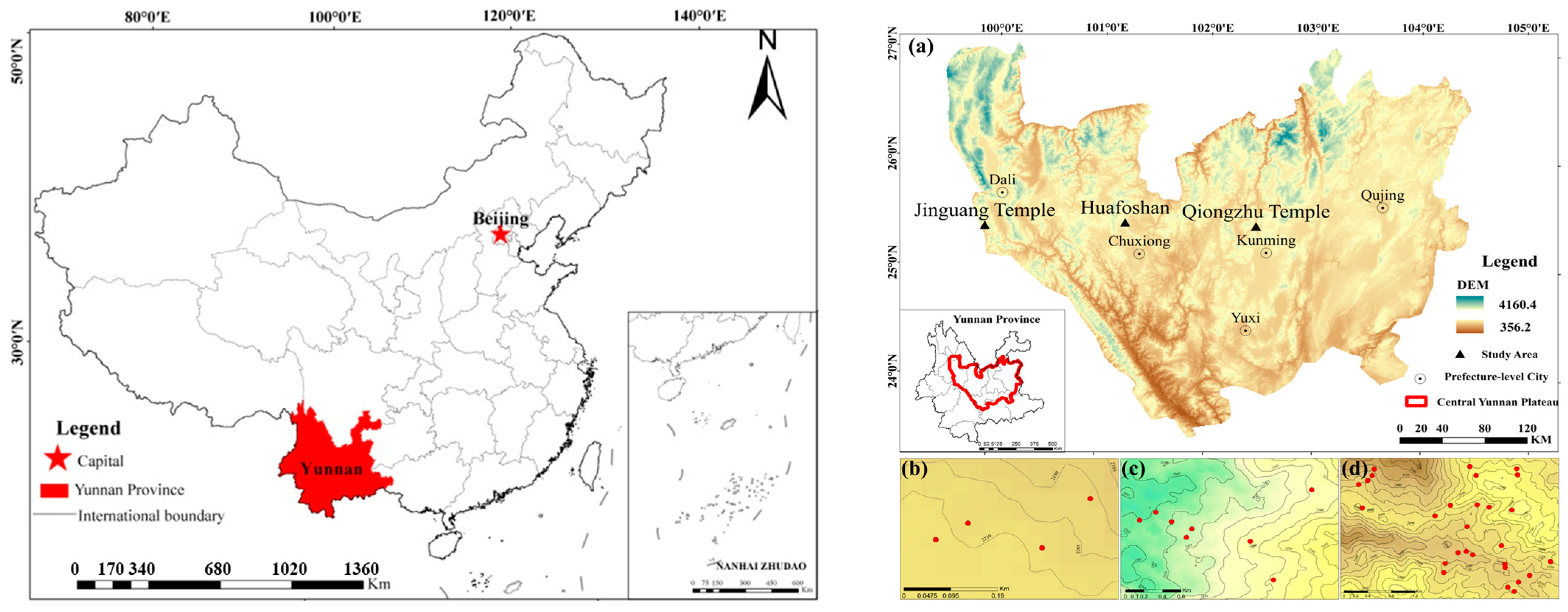
2. Materials and Methods

The CYP (ca. 23°19′~27°03′ N, 100°50′~104°43′ E) is located in the eastern-central part of Yunnan Province. The elevation ranges from 1500 m to 2500 m a.s.l. It has a semi-humid subtropical monsoon climate, with a strong seasonality in precipitation but not in temperature. The average annual temperature in this region is generally 18–24 °C, lower than in the same latitude locations in eastern China. The annual precipitation is about 800–1000 mm, with 85% occurring in summer and autumn, matched with a rather dry winter and spring [59]. The soil type is mainly red loam, with high weathering and low organic matter content [66]. Within the zonal vegetation of SBEFs, C. orthacantha (Fagaceae) is the most common community type. Except for the dominant species C. orthacantha, other common tree species include Lithocarpus dealbatus (Hook.f. & Thomson ex Miq.) Rehder (Fagaceae), Rhododendron delavayi Franch. (Ericaceae), P. yunnanensis (Pinaceae), and Schima argentea E.Pritz. (Theaceae). The shrub layer is mainly composed of Myrsine africana L. (Primulaceae), Vaccinium duclouxii (H.Lév.) Hand.-Mazz. (Ericaceae), Rhododendron siderophyllum Franch. (Ericaceae), Morella nana (A.Chev.) J.Herb. (Myricaceae), and Eurya japonica Thunb. (Pentaphylacaceae), and the herbs mainly comprise Ainsliaea yunnanensis Franch. (Asteraceae), Ophiopogon intermedius D.Don (Asparagaceae), and Carex baccans Nees (Cyperaceae), et al. In this study, we sampled the natural C. orthacantha forests at three sites across the CYP, i.e., Qiongzhusi in Kunming City, Huafoshanin in Chuxiong City, and Jinguangsi in Dali City. These three sites are all known for their well-preserved SEBFs by religious facilities. The locations of sampling points are shown in Figure 1.

A total of 42 sample plots with an area of 400 m² (20 m × 20 m) were set up in July and August 2019 in Jinguangsi Nature Reserve (30 plots), Huafoshan Nature Reserve (8 plots), and Qiongzhusi Forest Park (4 plots) to investigate SEBF communities with C. orthacantha as the dominant species. These forests are of roughly three age classes (or succession stages), mainly caused by the large-scale deforestation in the 20th century. Early in the 1960s, the nationwide “Iron and Steel Production Campaign” led to widespread deforestation and charcoal production for iron production, resulting in an upper age limit of 60–65 years for mature forests in most areas. In the 1980s, China started the construction of nature reserves, and the forests in many areas have been protected since then, resulting in the formation of middle-aged forest communities over 40 years old. In 2000, China implemented the “Natural Forest Protection” policy, which banned the logging of natural forests, but led to concentrated deforestation (including state-owned forests) before the policy was implemented, and created large areas of young forests about 25 years old [59].

We selected 3–6 trees with the largest diameter at breast height (DBH) in each sample plot, and extracted tree cores using a tree-ring drill. We counted the rings of the tree cores to determine the tree ages, and estimated the community age accordingly. Due to the differences in forest area among the three sampling sites, the surveyed samples included two mature and two middle-aged forest plots in Qiongzhusi; four mature and four middle-aged forest plots in Huafoshan; and nine mature, twelve middle-aged, and nine young forest plots in Jinguangsi. During the survey, all vascular plant species in the plots were recorded. For individuals with DBH ≥ 2.5 cm, the species name and vitality were recorded; the height was calculated using a laser rangefinder to measure both the horizontal and slant distances and then determined by the Pythagorean theorem to obtain the vertical height; the DBH was measured using a diameter tape; and the crown size (east–west width × north–south width) was measured. Saplings (DBH < 2.5 cm) were not measured for DBH. Instead, only their numbers were recorded. The distinction between trees and shrubs was based on the growth status of the trees at the time of measurement. Trees with a larger DBH and a distinct main trunk were classified as trees. For cases where classification was uncertain in the field, the life history information recorded in the China Plant Species Information Database was used as an auxiliary tool for judgment and verification. The shrub and herbaceous layers were documented with species names and quantities [67]. Specimens were collected for unknown species and brought back for taxonomic identification following references [68,69]. Species identification was accomplished by referencing “Flora of China” and “Flora of Yunnan” to examine plant specimens and photographs. Subsequently, the Latin binomials and life forms were verified on the official website of the “Scientific Database of China Plant Species” (https://db.kib.ac.cn/ (accessed on 5 July 2023)).

The geographic coordinates and elevation of the plots were measured following the GPS. The slope aspect and slope angle were measured using a compass. The slope angle is the average angle between the slope and horizontal surfaces, ranging from 0° to 90°. The slope aspect, ranging from 0° to 360°, was transformed into 0° (north)~180° (south) to better indicate the gradient of solar radiation, and the negative cosine of the aspect was calculated to transform the value range into [−1, 1].

At the center of each 10 m × 10 m quadrat of each plot, a soil sample of 0–10 cm depth was collected after moving the surface litterfall. Four soil samples were fully mixed to represent the plot of 20 m × 20 m. Soil samples were taken back to the laboratory, adequately air-dried at room temperature, ground, and then sieved through a 100 mesh sieve for the following experiments. The pH value, organic carbon, total nitrogen, effective phosphorus, and ion exchange capacity were measured with standard procedures. Soil pH was measured with a pH meter, and the water/soil mass ratio was 2.5:1. Soil organic carbon and total nitrogen were determined by the dry combustion method using an Elemental Analyzer (vario Macro cube, Elementar, Langenselbold, Germany). The effective phosphorus content was determined with the alkali fusion molybdenum antimony anti-spectrophotometric method [70,71]. The ion exchange capacity was measured with the ammonium acetate method.

Climate data were collected from 129 county meteorological stations of Yunnan Province for the period 1986–2015. We interpolated the station records to a raster data layer for each monthly mean temperature and precipitation value across the CYP at a spatial resolution of 100 m, using the Thin-plate Smoothing Splines interpolation model [72]. The climatic data of each forest plot was extracted from the raster climate data layers, based on the geographical coordinates. The required eco-climatic indices were calculated using the formulas in

Table 1. Description of the habitat features of sampling plots and the calculating algorithms.

Factor		Variable	Unit	Description of Method or Algorithm
ENV	Climate	MAP	mm	Mean annual precipitation of 1986–2015
		MAT	°C	Mean annual temperature of 1986–2015
		PET	°C	Potential evapotranspiration: 58.93 × ABT *; ABT = ΣTi/12; Ti, monthly mean temperature over 0 °C (assigned to 30 °C when Ti > 30 °C [73])
		PDQ	mm	Precipitation in the driest quarter, i.e., winter
		PER	°C/mm	Moisture index = PET/MAP
		TS	-	Temperature seasonality: SD (monthly mean temperature) × 100
	Topography	ASP	-	Cos(aspect), aspect ranges from 0 (north) to 180 (south)
		SLO	°	Slope angle
	Soil	S_PH	-	Soil pH
		S_C	g/kg	Soil organic carbon content
		S_N	g/kg	Soil total nitrogen
		S_I	cmol/kg	Soil cation exchange capacity
		S_P	g/kg	Soil total phosphorus
	Dominance of C. orthacantha	DCo	%	The proportion of the total basal area of C. orthacantha Castanopsis orthacantha Franch. in the total basal area of the tree layer in each plot
Age		AGE	Year	Three age classes: old (>60 yr), mediate (40–60 yr), young (25–40 yr)
Geographic distance		GEO	Km	Euclidean distance between two plots, calculated using geographical coordinates

* ABT: Annual Bio Temperature (°C).

.

In this study, the Bray–Curtis dissimilarity index based on species abundance data and the Sørensen index based on the presence/absence data were both calculated to measure the beta diversity of the C. orthacantha communities.

$$D_{Bray–Curtis}\left(j,k\right)={\displaystyle \frac{{\sum }_{i=1}^n|X_{ij}-X_{ik}|}{{\sum }_{i=1}^n|X_{ij}+X_{ik}|}},$$

(1)

where D_{Bray–Curtis} (j,k) represents the dissimilarity between the jth and kth plots, X_ij represents the number of specimens of the ith species in the jth plot, X_ik represents the number of specimens of the ith species in the kth plot, and the total number of species in the plot is n [74,75]. The Bray–Curtis index was calculated using the “vegdist” function in the “vegan” R package version 2.6-2 [76].

$$\mathrm{S}\mathrm{ø}\mathrm{r}\mathrm{e}\mathrm{n}\mathrm{s}\mathrm{e}\mathrm{n}={\displaystyle \frac{\max \left(b,c\right)+\mathrm{m}\mathrm{i}\mathrm{n}(b,c)}{2a+\min \left(b,c\right)+\mathrm{m}\mathrm{a}\mathrm{x}(b,c)}}$$

(2)

$$\mathrm{n}\mathrm{e}\mathrm{s}\mathrm{t}\mathrm{e}\mathrm{d}\mathrm{n}\mathrm{e}\mathrm{s}\mathrm{s}={\displaystyle \frac{\max \left(b,c\right)-\mathrm{m}\mathrm{i}\mathrm{n}(b,c)}{2a+\min \left(b,c\right)+\mathrm{m}\mathrm{a}\mathrm{x}(b,c)}}\times {\displaystyle \frac{a}{a+\min \left(b,c\right)}},$$

(3)

$$\mathrm{t}\mathrm{u}\mathrm{r}\mathrm{n}\mathrm{o}\mathrm{v}\mathrm{e}\mathrm{r}={\displaystyle \frac{\mathrm{m}\mathrm{i}\mathrm{n}(b,c)}{a+\min \left(b,c\right))}},$$

(4)

where a and b are the number of species in the two plots, respectively, and c is the number of species shared by the two plots. The Sørensen index was decomposed into two components, namely turnover and nestedness. The turnover index represents the species replacement, and nestedness characterizes the richness differences between the communities compared [77]. Beta diversity decomposition was implemented using the “betapart” package in R version 1.6 [78].

The species accumulation curve was used to describe the trend of increasing species richness with increasing sampling area [79]. This is calculated by randomly sampling a certain number of plots from all the plots that we surveyed and aggregating the number of species in these samples. The species accumulation curves of different age classes of C. orthacantha forests were plotted separately in a 20 m × 20 m plot. For the numbers of species within plots under an age class, a random sampling and put-back sampling approach was adopted. The mean and variance of samples were obtained by randomly selecting N samples from all samples under the same age class and calculating the total number of species in these N samples and repeating this 999 times. The process was repeated with different number of samples (N). Species–area curves for the three age classes were plotted using the “specaccum” function in the “vegan” R package [76].

Correlation coefficients between matrices were calculated using the Mantel test and partial Mantel test to evaluate the effects of geographical distance, and of environmental differences in terms of soil, topographic, and climatic conditions and community age class on beta diversity among communities [17,80]. Firstly, we calculated the geographic distance between two plots based on the geographic coordinates, using the “geosphere” package in R [81]. The environmental differences between the two plots were evaluated with the Euclidean distance. The climatic, soil, topographic variables and dominance of C. orthacantha were first standardized and then combined into a variable indicating environmental factors before calculation. After obtaining the distance matrices, the Mantel test was used to test the correlation between the environment matrix, geographic distance matrix, and beta diversity matrix with 999 permutations to obtain the correlation and significance level between the two variables. Because the geographic distance and environmental matrices are not independent of each other, the partial Mantel test was used to assess the correlation between the single distance matrix and the species beta diversity matrix. The above analysis was done with the “vegan” package in R [76]. For significance tests between species beta diversity among forests of the same age classes at different sites, a non-parametric rank-sum Wilcoxon test was used, which was calculated based on the “ggpubr” package version 0.6.0 in R [82].

A total of 220 vascular plant species were recorded in the survey sample, and their Latin names of the APG III system were used to query the family information of each species using the “plantlist” package version 0.8.0 in R [83]. The phylogenetic tree was then constructed using the “U.PhyloMaker” package based on the plant family information [84], generating a local phylogenetic tree with branch lengths [85,86,87], implemented in the “picante” package version 1.8.2 in R [88]. The NRI (net relatedness index) and NTI (net nearest taxa index) were used to assess the phylogenetic structure of the community. The NRI focuses on the phylogenetic structure at the community level in terms of the overall phylogenetic tree. The NTI, on the other hand, is studied from the end of the evolutionary branch, focusing on the affinities of species between communities, and is therefore susceptible to the influence of the end of the evolutionary tree branch [89,90]. The two functions “ses.mpd” and “ses.mntd” of the “picante” R package were used to calculate the phylogenetic structure of the community, through randomly sampling the species positions on the phylogenetic tree 999 times [91,92]. The specific calculation formula is as follows.

$$\mathrm{M}\mathrm{P}\mathrm{D}={\displaystyle \frac{1}{2}}\left({\sum }_{j=1}^{n_a}{X}_j\overline{d_{jb}}+{\sum }_{k=1}^{n_b}{X}_k\overline{d_{ka}}\right),$$

(5)

$$\mathrm{M}\mathrm{N}\mathrm{T}\mathrm{D}={\displaystyle \frac{1}{2}}\left({\sum }_{j=1}^{n_a}{X}_j{Mind}_{jb}+{\sum }_{k=1}^{n_b}{X}_k{Mind}_{ka}\right),$$

(6)

$$\mathrm{N}\mathrm{R}\mathrm{I}=-1\times {\displaystyle \frac{{MPD}_s-{MPD}_r}{\mathrm{S}\mathrm{D}\left({MPD}_r\right)}},$$

(7)

$$\mathrm{N}\mathrm{T}\mathrm{I}=-1\times {\displaystyle \frac{{MNTD}_s-{MNTD}_r}{\mathrm{S}\mathrm{D}\left({MNTD}_r\right)}},$$

(8)

where species j ≠ species k; $\overline{d_{jb}}$ represents the average paired phylogenetic distance between species j in quadrat a and all species in quadrat b; $\overline{d_{ka}}$ represents the average paired phylogenetic distance between species k in quadrat b and all species in quadrat a; n_a represents the number of species in quadrat a; n_b represents the number of species in quadrat b; X_j represents the relative abundance of species in quadrat a; X_k represents the relative abundance of species in quadrat b; Mind_jb represents the closest phylogenetic distance between species j in quadrat a and all species in quadrat b; and Mind_ka represents the closest phylogenetic distance between species k in quadrat b and all species in quadrat a. MPD_s are the Mean Phylogenetic Distances (MPD_s) of all species in the sample site, which is the average of the genetic distance of the species pairs in the observed sample. MPD_r is the mean spectral distance of all species under the zero model, and SD(MPD_r) is the standard deviation of the mean spectral distance under the random model. MNTD_s are the mean values of the distances between the phylogenetic points of the species within the survey community and the phylogenetic points of the nearest related species, MNTD_r is the expected value of the nearest phylogenetic distance under the null model, and SD(MNTD_r) is its standard deviation.

Statistical tests of differences in diversity indices among sites and different age classes were implemented using the Kruskal–Wallis test. The Kruskal–Wallis test allows for unequal sample sizes and provides a test for numerous independent sample comparisons based on the rank-sum test. The “kruskal.test” function was used to test for differences in the overall distribution, followed by multiple comparisons between groups using the “pairwise.wilcox.test” function of the “rstatix” R package version 0.7.2 [93]. Plotting was performed using the “ggplot2” package version 3.4.2 [94] in R.

3. Results

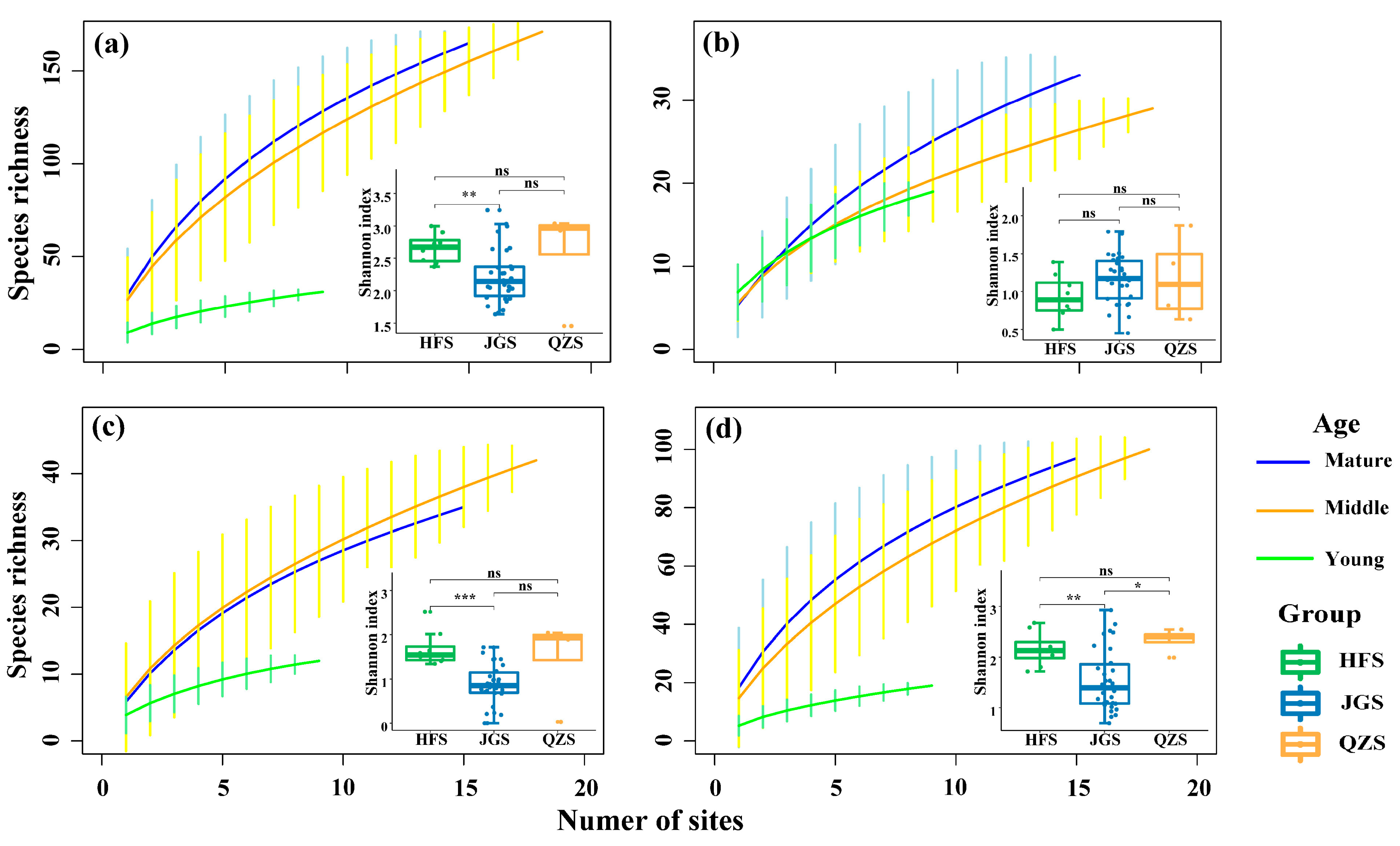
3.1. Plant Species Richness of Castanopsis Orthacantha Forests Across Sites and Age Classes

In a plot area of 400 m², the mean species richness was the highest in mature communities (27.5 ± 9.7 species), a little lower in the middle-aged communities (26.5 ± 10.3), and lowest in young communities (12.4 ± 5.7) (Figure 2). But for trees, the highest mean species richness was recorded in young communities (7.9 ± 3.7), that for shrub species was in middle-aged communities (6.8 ± 4.7), and the highest mean species richness for herbs was in mature communities (19.1 ± 7.6).

The species–area curves of the C. orthacantha forests showed that the rates of species richness increase with increasing plot number (and thus area) following the order of mature > middle > young communities (Figure 2a). Specifically, for both tree and herb species (Figure 2b,d), the increasing rates of species richness were generally highest in the mature communities and lowest in the young ones; whereas for shrubs (Figure 2c), the rate was highest in the middle-aged and lowest in the young communities.

The boxplots in Figure 2 indicate that, overall, plant species richness in the 400 m² plots was significantly higher (p < 0.05) at QZS (39.5 ± 10.6) and HFS (32.0 ± 10.3) than JGS (21.8 ± 10.0), but tree species richness did not statistically differ among plots at the three sites (JGS: 5.9 ± 1.6; HFS: 5.8 ± 1.2; QZS: 5.8 ± 0.8). The species richness of shrubs was significantly higher (p < 0.01) at QZS (11.0 ± 2.1) than HFS (8.3 ± 2.9), and both had a higher level (p < 0.01) than that at JGS (4.6 ± 2.4). Similarly, herb species richness in plots of a 400 m² area were the highest at QZS (24.8 ± 5.6), lower at HFS (18.0 ± 8.6), and lowest at JGS (11.5 ± 8.6) (p < 0.05).

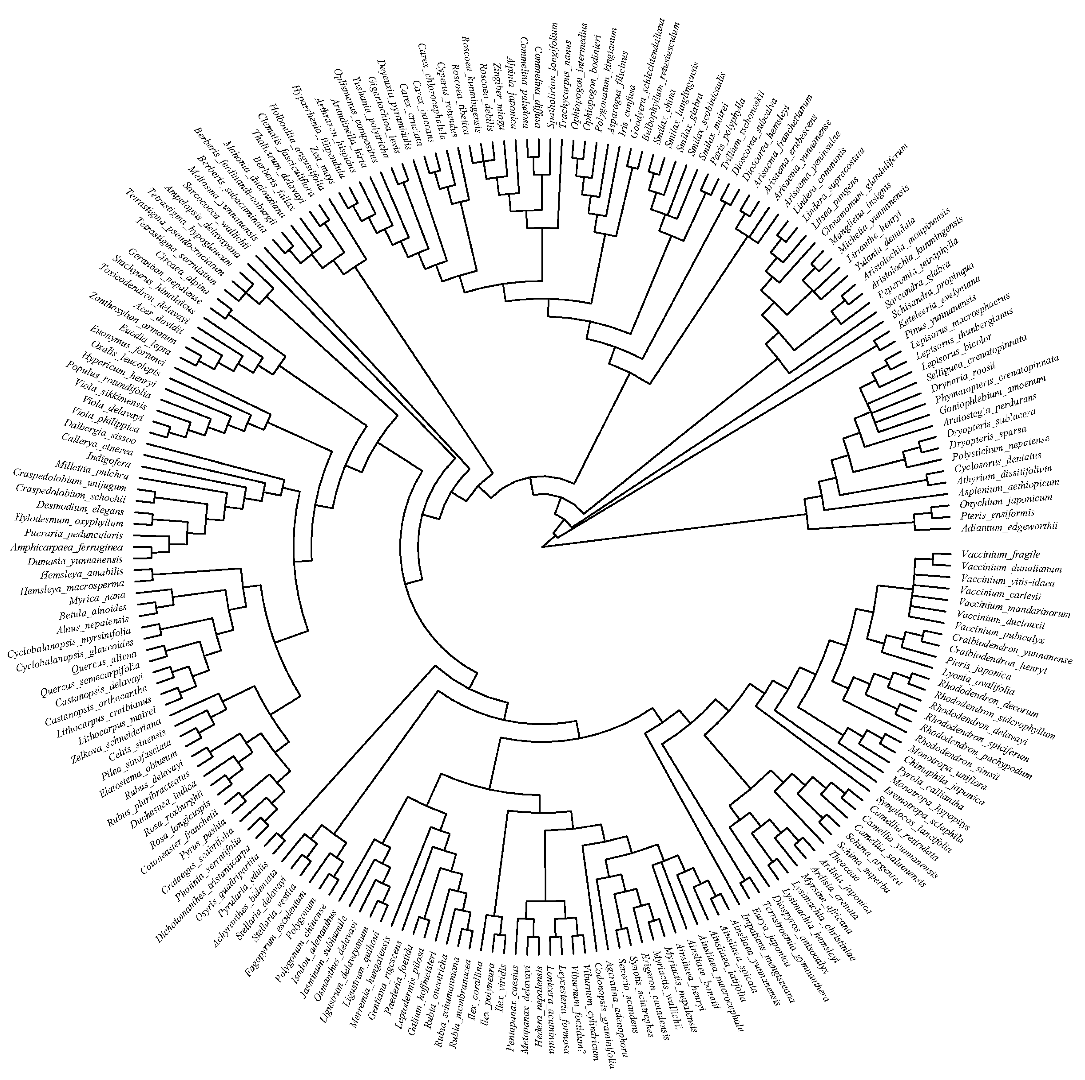
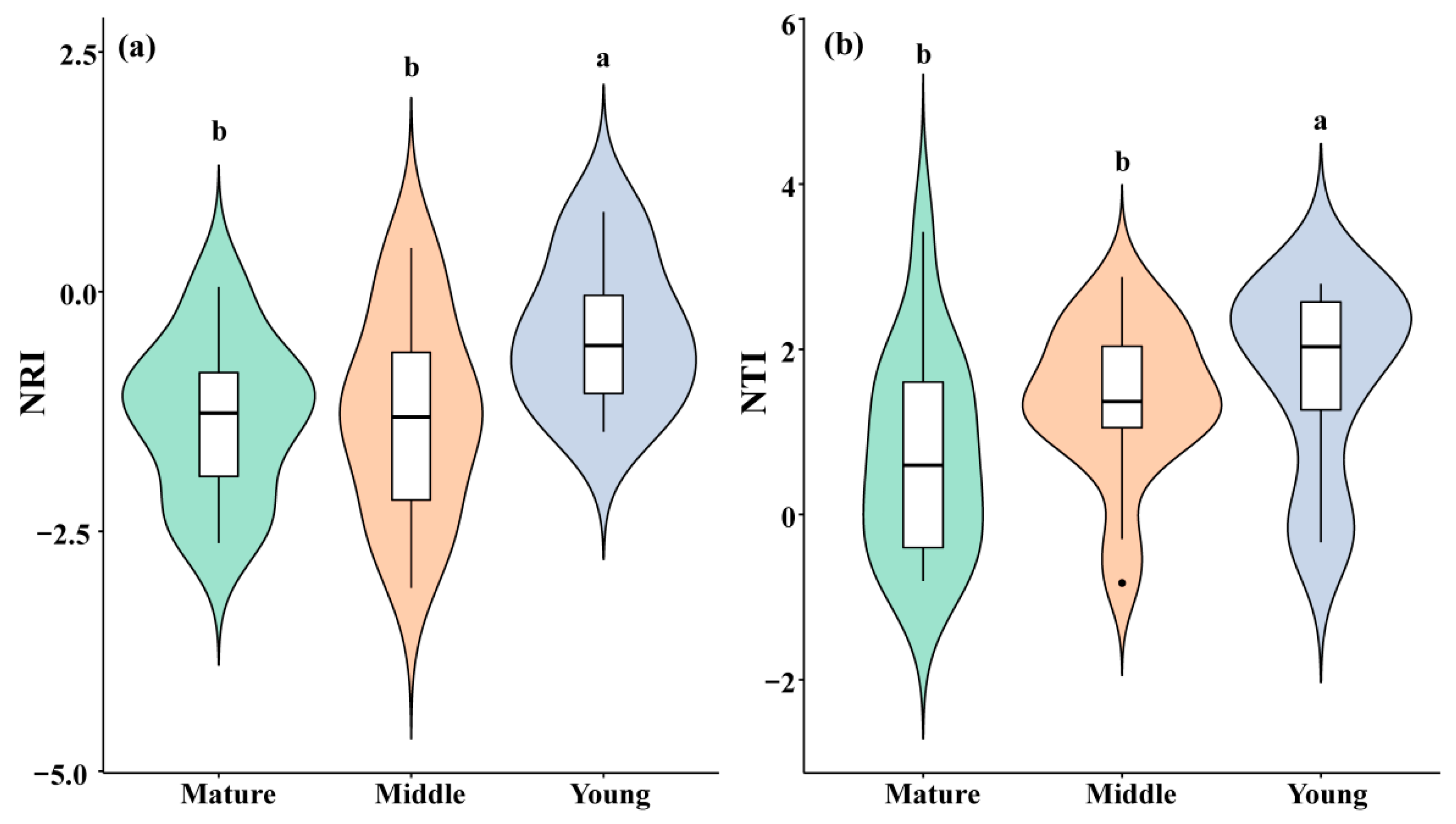
3.2. Phylogenetic Structure of Communities of Different Age Classes

The NRI of the C. orthacantha communities of the three age classes decreased from the young (−0.426 ± 0.258) to the middle (−1.312 ± 0.210) and to the mature forests (−1.289 ± 0.244), suggesting that the phylogenetic community structure is more over-dispersed in the mature forests (Figure 3a). The trend of the NTI value was similar to that of the NRI. Also, it decreased with increasing community age class (i.e., 1.697 ± 0.389 for the young, 1.386 ± 0.222 for the middle-aged, and 0.719 ± 0.313 for the mature communities), showing an over-dispersion trend of phylogenetic structure with an increase in community age.

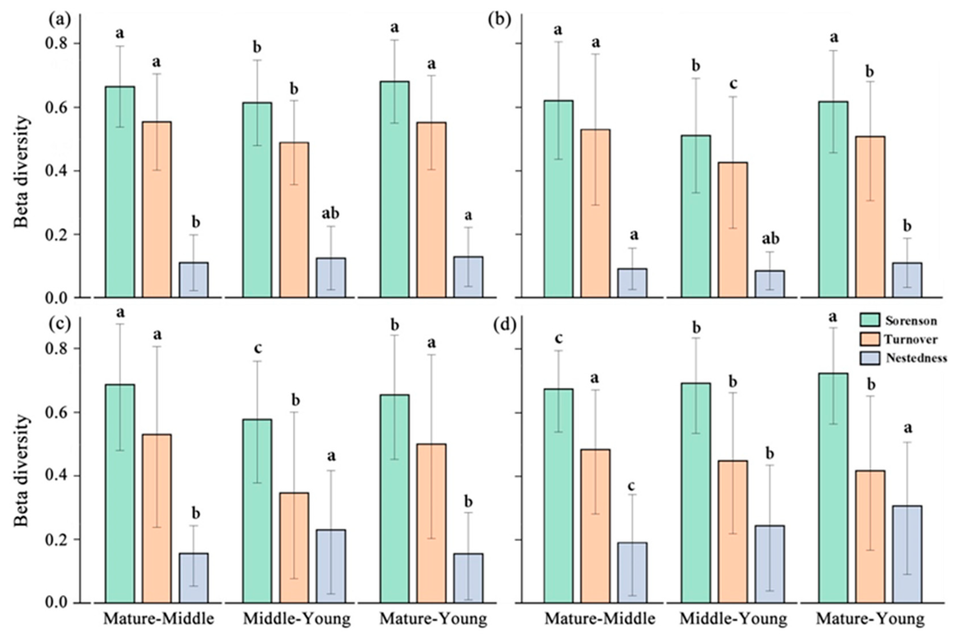
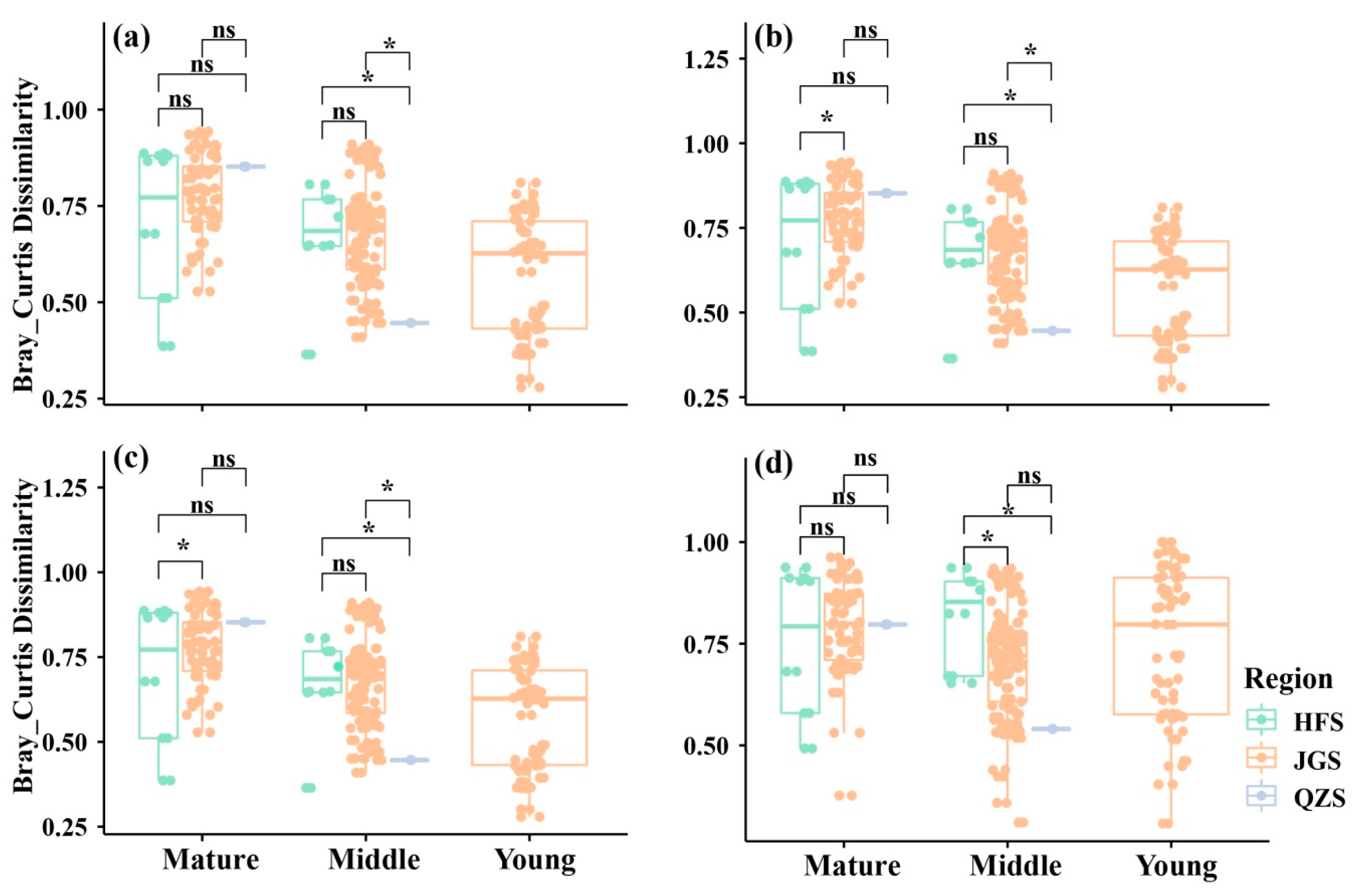
3.3. Temporal and Spatial Patterns of Community Beta Diversity and Its Components

The results of beta diversity and its decomposition in the tree, shrub, and herb layers showed that the turnover component dominated under all three forest age classes. For all species (Figure 4a) and within the tree layer (Figure 4b), the turnover component was much larger than the nestedness component, accounting for about 81–84% of the total. The turnover fractions were slightly lower in the shrub and herb layers, accounting for about 66.2–72.6% of the overall diversity fraction. The Sørensen index of the tree layer was the lowest (0.597 ± 0.005), and the beta diversity index of the herb layer was the highest (0.646 ± 0.006). The beta diversity decomposition components of the community also changed in different succession stages, and the change in component proportion is more eminent in the shrub and herb layers (Figure 4c,d). The largest proportion of species replacement in the shrub and herb layers occurred between mature and middle-aged forests, and the change in the species replacement proportion in tree layers in different forest ages is not obvious (Figure 4b).

It can be seen from the results in Figure 5 that in the mature forests, QZS (0.852 ± 0.001) and JGS (0.780 ± 0.127) have the highest beta diversity, and there is no significant difference between them, while JGS and HFS (0.701 ± 0.589) have significant differences. In middle-aged communities, the difference in beta diversity between sites showed an opposite trend, with the lowest beta diversity in QZS, indicating that the difference in species composition between middle-aged forests in QZS was smaller than the difference in species richness between sites in JGS and HFS.

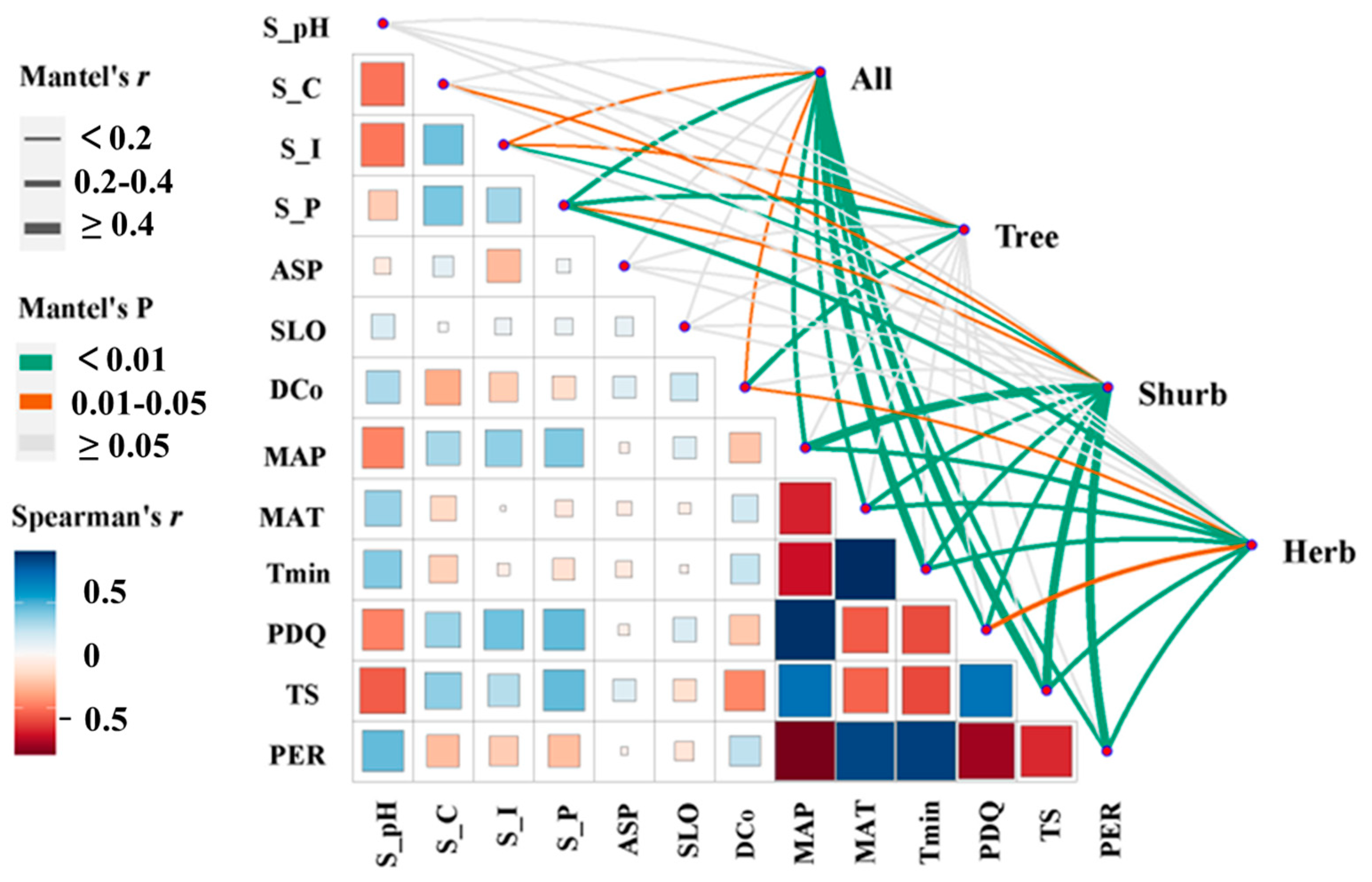
3.4. Driving Factors of Forest Beta Diversity Patterns at Tree, Shrub, and Herb Layers

The Mantel test and the partial Mantel test reflected the correlation between the matrix of beta diversity of the C. orthacantha communities, the matrix of geographical distance among sites, and the distance matrices of environmental factors, including soil, climate, and topography (

Table 2. The Mantel test and partial Mantel test between the beta diversity of C. orthacantha communities (including all species and that of the specific tree, shrub, and herb layers) and environmental factors.

Variables	All Species		Tree Layer		Shrub Layer		Herb Layer
	Sørensen	Bray	Sørensen	Bray	Sørensen	Bray	Sørensen	Bray
GEO	0.617 ***	0.544 ***	0.532 ***	0.404 ***	0.485 ***	0.562 ***	0.443 ***	0.429 ***
ENV	0.592 ***	0.557 ***	0.462 ***	0.385 **	0.550 ***	0.590 ***	0.363 ***	0.409 ***
Climate	0.576 ***	0.515 ***	0.439 ***	0.288 **	0.491 ***	0.533 ***	0.405 ***	0.414 ***
Soil	0.278 **	0.303 ***	0.223 **	0.263 **	0.312 **	0.299 **	0.113	0.211 **
TOPO	0.066	0.092	0.090	0.125 *	0.039	−0.009	0.040	0.059
AGE	0.054	0.122 *	0.060	0.215 **	0.029	0.009	0.072	0.074 *
GEO|ENV	0.355 ***	0.263 ***	0.331 ***	0.207 **	0.172 *	0.263 ***	0.285 ***	0.220 **
ENV|GEO	0.289 **	0.298 *	0.153 *	0.159 *	0.339 **	0.337 *	0.137 *	0.172 *
Climate|GEO	0.227 **	0.196 *	0.075	−0.023	0.222 **	0.205 *	0.124 *	0.157 *
Soil|GEO	0.205 **	0.239 **	0.143	0.205 **	0.254 **	0.223 **	0.081	0.144 *
TOPO|GEO	0.050	0.082	0.079	0.118	0.020	0.040	0.023	0.045
AGE|GEO	−0.008	0.042	0.009	0.193 **	−0.020	−0.055	0.032	0.036
AGE|Climate	0.096	0.132 *	0.088	0.250 ***	0.061	0.040	0.092	0.098

*: 0.01 ≤ p < 0.05; **: 0.001 ≤ p < 0.01; ***: p < 0.001.

). Based on the Sørensen index, there was a significant positive correlation between beta diversity in the tree layer and geographical distance and climate (r = 0.331, p < 0.001; r = 0.153, p < 0.001); the herb layer also presented a significant correlation (r = 0.285, p < 0.001; r= 0.131, p < 0.001). The correlation of beta diversity with the environment in the shrub layer was larger than that with geographical distance (r = 0.339, p < 0.001). Based on the Bray–Curtis index, the correlation with age class was significantly stronger in the tree layer (r = 0.250, p < 0.001), and the correlations with environmental variables were not significantly different from the previous index.

The Sørensen index is based on species presence/absence and the Bray–Curtis index is measured with species abundance. In general, the correlations between beta diversity based on the Sørensen index and spatial or environmental distance matrices were generally stronger than the correlations between the Bray–Curtis index and spatial/environmental distances.

According to the heat map of the Spearman’s r index among specific environmental variables (Figure 6), high correlations existed among climate variables, especially MAT, MAP, and PDQ. Combined with the results of the Mantel test (Figure 6;

Table A1. Matrix heat map of the Mantel tests.

Environmental Variables	Beta Diversity
	Community	Tree Layer	Shrub Layer	Herb Layer
S_PH	0.027	−0.041	0.087	−0.003
S_C	0.126	0.064	0.142 **	0.063
S_I	0.148 *	0.170 *	0.169 ***	0.044
S_P	0.278 ***	0.235 **	0.174 **	0.234 **
ASP	0.028	0.034	0.028	0.017
SLO	−0.029	0.027	−0.078	−0.078
DCo	0.151 *	0.315 ***	0.015	0.166 *
AP	0.069	0.092	0.415 ***	0.246 ***
MAT	0.349 ***	0.062	0.339 ***	0.271 ***
Tmin	0.400 ***	0.072	0.372 ***	0.291 ***
PDQ	0.313 ***	0.098	0.375 ***	0.225 **
TS	0.456 ***	0.149	0.443 ***	0.365 ***
PER	0.396 ***	0.074	0.434 ***	0.283 ***

*: 0.01 ≤ p < 0.05; **: 0.001 ≤ p < 0.01; ***: p < 0.001.

), significant and positive correlations were also revealed between the beta diversity of all species among C. orthacantha communities and the difference in soil total phosphorus content (S_P) (r = 0.278, p < 0.001), MAT (r = 0.349, p < 0.001), the mean coldest monthly temperature (Tmin) (r = 0.400, p < 0.001), temperature seasonality (TS) (r = 0.456, p < 0.001), and the dominance of the C. orthacantha population (DCo) (r = 0.151, 0.01 ≤ p < 0.05). In particular, the beta diversity of tree species showed significant positive correlations with differences in DCo (r = 0.315, p < 0.001) and S_P (r = 0.235, p < 0.001); the beta diversity of the shrub layer showed highly significant correlations with differences in all climatic and some soil variables (S_P, S_I). There was also a highly significant correlation between beta diversity in the herb layer and differences in climatic variables, soil total phosphorus content (r = 0.234, 0.001 ≤ p < 0.01), and DCo (r = 0.166, 0.001 ≤ p < 0.05), as well.

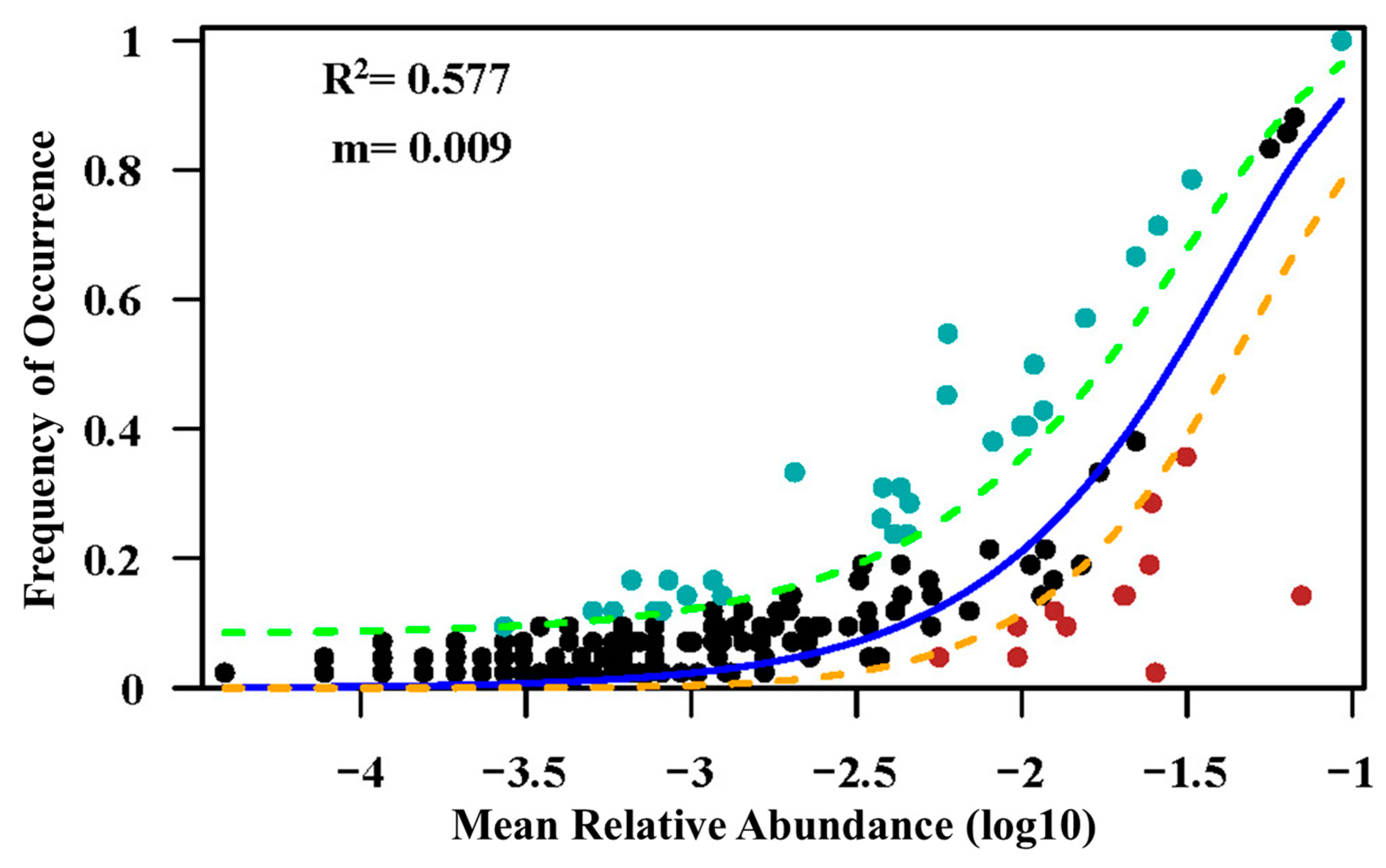
3.5. Determination of Forest Community Assembly at Local and Regional Scales

Correlations between the beta diversity matrices, at both inter-site and intra-site scales, with environmental distance, spatial distance, and community age class (successional stage) are shown in

Table 3. Mantel test between community beta diversity and explanatory variables at different scales.

Variables	Inter-Sites		Intra-Site
	Sørensen	Bray	Sørensen	Bray
GEO	0.579 ***	0.375 ***	0.165 *	0.294 ***
ENV	0.531 ***	0.205 *	0.244 ***	0.308 ***
Climate	0.508 ***	0.153 *	0.22 ***	0.261 ***
Soil	0.068	0.100	0.215 ***	0.230 ***
TOPO	0.087	0.167 *	0.186 **	0.255 ***
AGE	0.115 *	0.127 *	0.019	0.184 **
GEO|ENV	0.393 ***	0.355 ***	0.141 *	0.287 ***
ENV|GEO	0.315 ***	0.180 **	0.196 **	0.234 ***
Climate|GEO	0.301 ***	−0.131	0.172 **	0.243 ***
Soil|GEO	0.002	0.064	0.170 **	0.221 ***
TOPO|GEO	0.051	−0.107	0.159 *	0.238 ***
AGE|GEO	−0.049	0.051	−0.024	0.127 *
AGE|Climate	0.184 **	0.144 *	0.019	0.202 ***

*: 0.01 ≤ p < 0.05; **: 0.001 ≤ p < 0.01; ***: p < 0.001.

. At the inter-site scale, the beta diversity values of the Sørensen index, which is based on presence/absence data, were generally larger than those of the Bray–Curtis index, which is based on species abundance data; and the opposite generally applies, at the intra-site scale, for the results of both the Mantel test and the partial Mantel test.

At the inter-site scale, the correlations of both indices of beta diversity with spatial distance were stronger than those with environmental variables, and the correlation was weakest with age class. In particular, climate dominated the role of environmental difference when only species presence/absence (i.e., Sørensen index) was considered, while topography played a larger role than climate when the population information of species was taken into account (i.e., Bray index). The effects of spatial, environmental, and age factors on community beta diversity were also mostly revealed by the partial Mantel test. However, when geographical distances were controlled, only the effects of climate differences were significant in the Sørensen index, and no significant effects were found for climate, topography, soil, or even community age in the Bray index.

At the intra-site scale, correlations of community beta diversity (in both indices) with environmental differences were stronger than with spatial distance or community age class. In particular, correlations of the Sørensen index with differences in climate, soil, and topography were all significant and larger than those with geographical distances or age differences, although the effect of spatial distance became stronger when population abundance was taken into account. The partial Mantel test suggested that the effect of environmental difference on the Sørensen index with spatial distance controlled was larger than the effect of spatial distance with environment controlled, but the opposite applied for the Bray index. The effect of community age was the weakest at this scale, and was significant only for the Bray index with the spatial or environmental effect controlled.

4. Discussion

In this study, we analyzed the changes in taxonomic alpha diversity and beta diversity, and phylogenetic structure of the SEBF communities at three sites in the CYP with C. orthacantha as the dominant species, and quantified the contributions of environmental, spatial, and temporal factors to the assembly within and across local communities. The results show that there is a significant scale dependence on the effects of different community assembly mechanisms for this fragmented distribution of forest types. As community succession advances, species richness within the community exhibits an initial increase followed by a trend towards stabilization. Phylogenetic structure, on the other hand, transitions from random to dispersion patterns.

4.1. Differences in Beta Diversity at Different Spatial Scales and Their Drivers

Environmental gradients, interactions between organisms, and dispersal limits are important factors in shaping C. orthacantha community structure at different scales [95], and there is a strong correlation with spatial distance. The spread of species is highly correlated with spatial distance, which, as an indicator of the limitations on species dispersal, is widely utilized in research on spatial turnover [96,97]. The beta diversity among the three sampling areas in this study consistently exceeded that within each individual area, in alignment with the findings of previous research [98]. This study analyzes the proportional changes of beta diversity decomposition components across three succession stages, indicated by age classes. An overall successional trend emerges: regardless of the different strata of trees, shrubs, herbs, or various forest ages, the turnover component constitutes a larger proportion. It is generally believed that dispersal barriers between different geographical regions often lead to nestedness differences in species composition [99]. When the habitat differences among regions exceed the internal variations within individual sites, it tends to drive the replacement of species composition at large spatial scales [100]. According to the relevant literature, regions that experienced a warm climate during the Quaternary period maintained stable climatic conditions, which safeguarded species from extinction and facilitated speciation within these areas. As a result, warmer regions, in contrast to those with colder climates, exhibit a greater richness of narrow-range species [101]. As a result, the decomposition of species beta diversity reveals that the turnover rate is predominant, indicating a significant contribution to the overall pattern of biodiversity change [102]. The results of our investigation reveal the patterns of beta diversity variations across distinct forest age classes. Specifically, within the shrub and herb layers, the proportion of species turnover is pronounced during the transition from middle to old age classes, whereas an increment in nestedness is observed in the progression from young to middle-aged and mature forests. These patterns imply that the succession of the forest community, from early to late stages, is marked by an initial phase where changes in species richness are prevalent, succeeded by a subsequent phase characterized by a higher frequency of species replacement. We posit that this observation can be attributed to the later phases of community assembly, during which, after the establishment of a stable tree canopy, understory species that are shade-intolerant and sunlight-dependent progressively diminish in abundance, thereby facilitating species turnover within the community composition.

The results of our study indicate that the correlation between spatial distance and inter-site variation in community-level species composition is most pronounced. Our findings underscore the importance of dispersal limitations at larger scales, where long-distance dispersal becomes challenging for certain species, thus corroborating our initial hypothesis presented at the outset of this article. This finding is also consistent with previous studies that investigated the relationship between plant community turnover and geographic distance, such as research on the tropical monsoon rainforest in Argentina [96], the rainforests in the southern Amazon [103], and the succession of temperate northern forests in Canada [44]. Contrary findings have also been reported, such as the comparative study of the Gutian Mountains in China and the BCI large sample plots in Panama, in which, as the sampling particle size increased, the contribution of geographic distance gradually decreased, while the correlation between topography and dissimilarity gradually strengthened. It is important to note that this research was conducted at a scale limited to within a single plot (<800 m). In addition, studies on tropical forests have found weak to no effects of geographical distance on fern composition in tropical forests [26], and there may also be a problem with the small scale of the study area (<2000 m). When the scale of the study is not large enough, the influence of dispersal limitation, as represented by geographic distance, may remain undetected in terms of its effect on species composition, especially for vascular plants with broad ranges within the study region [104]. The maximum distance between the two regions in this study is within the range of about 300 km, which just verifies the previous view at this scale. This conclusion proves to some extent that the neutral theoretical solution can explain part of the variation in communities. We employed a neutral community model to validate our hypothesis, as illustrated in Appendix A Figure A2. The results indicate that the neutral community model adequately describes the relationship between species occurrence frequency and relative abundance (R² = 0.577). However, it does not mean that the world is neutral, only that dispersal limitation is a key link in the process of influencing community assembly [105].

The influence of climate variables as key environmental factors on the spatial variation of plant communities is widely confirmed [6,106]. Temperature and precipitation form climatic gradients across different study plots, and while these inter-regional climatic gradients do not result in drastic shifts in species composition, they do drive changes in species richness between regions. These findings have been confirmed in both temperate and tropical forests [107,108]. For the C. orthacantha community in this study area, the limiting climatic conditions, such as PER, TS, and PDQ, had a greater influence on the beta diversity among shrubs and herbs, while the similarity index of tree layers did not correlate well with the climatic variables. At large scales, environmental variables, particularly climatic ones, exhibit a significant positive correlation with the dissimilarity of community composition. Numerous studies have demonstrated that indices measuring community species turnover typically increase with the dissimilarity of climatic variables [109,110]. Our results show that climate variables are positively correlated with the community dissimilarity index at both large and local scales. Compared to spatial distance, environmental variables have a stronger influence on beta diversity at the intra-site scale, which is consistent with the hypothesis we proposed at the beginning of the article.

Topographic heterogeneity produces soil variability in drainage and nutrient deposition between soil types [111] and creates geographic isolation on small scales; most soil physicochemical properties characterize differences in soil nutrient content. In tropical and temperate forest ecosystems, variations in ecological niches, which are correlated with environmental factors such as topography and soil characteristics, have been identified as significant determinants of species distribution at both local and landscape scales [112,113]. In the study area, soil nutrients (S_P, S_I) significantly contribute to the dissimilarity across the tree, shrub, and herb layers, and aspect also plays a role in local environmental heterogeneity. At the finer scale of small plots, local environmental variables such as topography (aspect) and soil nutrients exhibit independent effects (controlling for spatial distance), suggesting that at more refined spatial scales, environmental factors such as topography and soil may influence the composition and richness of understory plants in regions with relatively low spatial heterogeneity, thereby inducing small-scale niche constraints [114,115].

As a result, at the inter-sites scale, dispersal limitation emerges as the predominant driver of community beta diversity. Among environmental variables, climatic factors contribute significantly, albeit to a slightly lesser extent than spatial distance, whereas their influence on community heterogeneity substantially surpasses that of topographical and soil variables. The relative contributions of these factors are as follows: spatial distance > environmental variables > community forest age. Within the three study sites, at the intra-site scale, the correlation between environmental variables, such as soil and topography, and beta diversity is heightened. Notably, certain restrictive climate variables, including PDQ, TS, and PER, are prominent. The levels of contribution from these three types of factors are comparable, with the pattern at smaller spatial scales indicating that environmental filtering, encompassing climate, topography, and soil, predominates over spatial distance, suggesting that environmental variables are key determinants of community assembly. Furthermore, at larger scales, the Sørensen index exhibits strong associations with the various variables, while at finer scales, the Bray–Curtis index, derived from abundance data, demonstrates superior performance.

4.2. Main Drivers of Different Community Assembly Stages

The results of this study showed that the early stage of community assembly is the accumulation stage of species richness, so the species richness in the young (10–15 years) stage is lower than the richness in the middle-aged forest, while the species richness in the middle-aged forest (25–44 years) and the mature forest (45–65 years) are very similar, which is similar to the results of studies in tropical secondary forest areas [116]. During the mid-to-late stages of community succession (from middle-aged to mature forests), a trend towards stability is observed, with the rate of increase in species richness within the community slowing under conditions of minimal disturbance. Considering the differences in species richness across successional stages, it can be inferred that the transition from young to middle-aged forests represents the phase of most rapid change in community composition and richness for the C. orthacantha community, primarily evident in the shrub and herb layers, whereas changes in the tree layer are less pronounced. Subsequently, during the transition from middle to late successional stages, the rate of species richness change gradually declines. Given the relatively broad age group intervals employed in this study, it is not possible to pinpoint the exact timing of rapid community accumulation. Future research could address this limitation by subdividing the communities into finer age groups to investigate the specific age stages at which dramatic changes in community structure occur.

The age of a community is closely associated with a range of ecosystem service functions, including net primary productivity and carbon cycling [117,118]. Based on the results of the Mantel test conducted in this study, forest age emerges as a significant predictor of variations in community richness and species composition. Age-related differences, primarily manifested in the tree layer, can alter understory conditions such as light and moisture, thereby exerting a considerable influence on the herbaceous layer. The results of the phylogenetic structure index (NRI) indicate that the phylogenetic community structure of middle-aged and mature forests exhibits an over-dispersion pattern, whereas that of young forests is characterized by phylogenetic randomness. Results from the analysis of the NRI reveal that the phylogenetic structure of communities within middle-aged and mature forest stages demonstrates a pattern of phylogenetic over-dispersion, whereas the young forest stage is indicative of a random distribution. These findings are concordant with previous research, wherein investigators have categorized tree communities into five distinct age classes based on diameter class structure, observing that the phylogenetic structures of smaller diameter classes exhibit either clustering or randomness, whereas those of larger diameter classes tend to diverge [119,120]. Additionally, research on the phylogenetic structure across different successional stages has also revealed that as succession progresses, the phylogenetic structure tends to become more over-dispersive, with communities of larger diameter classes exhibiting greater over-dispersion [121]. The possible explanation for this phenomenon is that seed dispersal from parent trees is limited, leading to clumped growth of seedlings and saplings in young forests, and, thus, the community, as a whole, exhibits phylogenetic clustering. As trees grow larger, competition among individuals intensifies, and the geographic distance between surviving species increases, resulting in an overall phylogenetic over-dispersion [122].

4.3. Recommendations on the Protection of Zonal Forest Vegetation

In the context of habitat fragmentation and rapid global climate change, a comprehensive and fine-grained understanding of changes in the diversity of different communities is essential. Previous studies have pointed out that there are gaps in the study of evergreen broadleaved forest woody plant conservation in China [123]. Our paper measures the diversity of C. orthacantha forest, a representative of semi-zonal vegetation in central Yunnan’s SEBF community, through multiple levels including dimension indicators and different spatial and temporal scales, providing key data to support the subsequent conservation of this forest type.

To understand the interaction between species diversity variations at different dimensions and environmental gradients, stochastic processes should be taken into consideration for the conservation of C. orthacantha communities in the research area [124]. To implement different conservation measures in combination with the age of the forest targeted, especially for communities in the early stages of succession, previous studies found that in some forest types, uneven age management yielded greater environmental benefits than community conservation without considering the age. In order to maintain species richness within local habitats, forest management should prioritize areas with high environmental variability and create high local habitat heterogeneity (including topography, soil nutrients, climate, etc.) to ensure high species diversity. When implementing conservation on a larger scale, it is important to fully consider distance, spatial barriers, and plant propagule dispersal capacity, in addition to maintaining high environmental heterogeneity. In summary, appropriate conservation programs should be developed for the age, geographic location, and position in the community of the conservation object.

4.4. Research Limitations and Perspectives for Future Exploration

Our study focuses on Castanopsis orthacantha forests in the Central Yunnan Plateau, a representative group of semi-humid evergreen broad-leaved forests. Although the surveys span across distinct sites, the geographic scope remains relatively confined. Expanding the spatial scale across the broader distribution range could provide a more comprehensive view. Further research on other types of SEBFs would also boost our understanding of diversity patterns and mechanisms under community assembly. In addition to well-preserved forests such as the ones we surveyed, future research into communities affected by climate change and human activities could provide more insight into the preservation of SEBFs. Future studies aiming to integrate multi-scale, multidimensional approaches will provide a more holistic understanding of the dynamics of biodiversity and community assembly, enabling more effective conservation and restoration strategies for fragmented forest ecosystems.

5. Conclusions

This study highlights the roles of spatial distance, environmental differences, and community age in shaping the plant diversity patterns in fragmented Castanopsis orthacantha forests across the Central Yunnan Plateau. Our findings reveal that community assembly processes are scale-dependent and vary substantially with successional stages. Specifically, spatial distance and dispersal limitation dominate community assembly at larger spatial scales, while environmental filtering plays a more significant role at local scales. Community age influences taxonomic and phylogenetic diversity, with phylogenetic clustering in early successional stages and a transition to over-dispersion in later stages, reflecting shifts in community assembly mechanisms from environmental filtering to competitive exclusion and niche differentiation.

The decomposition of beta diversity into turnover and nestedness components further illustrates that species replacement is the key driver of compositional variation across sites and age classes, particularly during transitions between successional stages. These results emphasize the importance of integrating spatial, environmental, and temporal factors to fully understand the dynamics of community assembly and biodiversity maintenance. From a conservation perspective, our findings underline the necessity of prioritizing environmental heterogeneity and addressing dispersal limitations to restore and conserve fragmented semi-humid evergreen broad-leaved forests effectively.

References

1. Gaston, K.J. Global patterns in biodiversity. Nature 2000, 405, 220–227. [Google Scholar] [CrossRef]
2. Tang, Z.; Wang, Z.; Fang, J. Historical hypothesis in explaining spatial patterns of species richness. Biodivers. Sci. 2009, 17, 635–643. [Google Scholar]
3. Socolar, J.B.; Gilroy, J.J.; Kunin, W.E.; Edwards, D.P. How Should Beta-Diversity Inform Biodiversity Conservation? Trends Ecol. Evol. 2016, 31, 67–80. [Google Scholar] [CrossRef] [PubMed]
4. Whittaker, R.H. Evolution and Measurement of Species Diversity. TAXON 1972, 21, 213–251. [Google Scholar] [CrossRef]
5. Whittaker, R.H. Vegetation of the Siskiyou Mountains, Oregon and California. Ecol. Monogr. 1960, 30, 280–338. [Google Scholar] [CrossRef]
6. Condit, R.; Pitman, N.; Leigh, E.G.; Chave, J.; Terborgh, J.; Foster, R.B.; Núñez, P.; Aguilar, S.; Valencia, R.; Villa, G.; et al. Beta-diversity in tropical forest trees. Science 2002, 295, 666–669. [Google Scholar] [CrossRef]
7. Kraft, N.J.B.; Comita, L.S.; Chase, J.M.; Sanders, N.J.; Swenson, N.G.; Crist, T.O.; Stegen, J.C.; Vellend, M.; Boyle, B.; Anderson, M.J.; et al. Disentangling the Drivers of β Diversity Along Latitudinal and Elevational Gradients. Science 2011, 333, 1755–1758. [Google Scholar] [CrossRef] [PubMed]
8. Anderson, M.J.; Crist, T.O.; Chase, J.M.; Vellend, M.; Inouye, B.D.; Freestone, A.L.; Sanders, N.J.; Cornell, H.V.; Comita, L.S.; Davies, K.F.; et al. Navigating the multiple meanings of β diversity: A roadmap for the practicing ecologist. Ecol. Lett. 2011, 14, 19–28. [Google Scholar] [CrossRef] [PubMed]
9. Carroll, C.; Roberts, D.R.; Michalak, J.L.; Lawler, J.J.; Nielsen, S.E.; Stralberg, D.; Hamann, A.; Mcrae, B.H.; Wang, T.L. Scale-dependent complementarity of climatic velocity and environmental diversity for identifying priority areas for conservation under climate change. Global Change Biol. 2017, 23, 4508–4520. [Google Scholar] [CrossRef] [PubMed]
10. Li, G.; Xiao, N.W.; Luo, Z.L.; Liu, D.M.; Zhao, Z.P.; Guan, X.; Zang, C.X.; Li, J.S.; Shen, Z.H. Identifying conservation priority areas for gymnosperm species under climate changes in China. Biol. Conserv. 2021, 253, 108914. [Google Scholar] [CrossRef]
11. Weiher, E.; Keddy, P.A. Assembly Rules, Null Models, and Trait Dispersion—New Questions Front Old Patterns. Oikos 1995, 74, 159–164. [Google Scholar] [CrossRef]
12. Fernandez-Going, B.M.; Harrison, S.P.; Anacker, B.L.; Safford, H.D. Climate interacts with soil to produce beta diversity in Californian plant communities. Ecology 2013, 94, 2007–2018. [Google Scholar] [CrossRef] [PubMed]
13. Gause, G. The Struggle for Existence; Dover Publications: New York, NY, USA, 2003. [Google Scholar]
14. Hubbell, S. The Unified Neutral Theory of Biodiversity and Biogeography; Princeton University Press: Princeton, NJ, USA, 2001. [Google Scholar]
15. Soininen, J.; McDonald, R.; Hillebrand, H. The distance decay of similarity in ecological communities. Ecography 2007, 30, 3–12. [Google Scholar] [CrossRef]
16. Litvak, M.K.; Hansell, R.I.C. A Community Perspective on the Multidimensional Niche. J. Anim. Ecol. 1990, 59, 931–940. [Google Scholar] [CrossRef]
17. Tuomisto, H.; Ruokolainen, K.; Yli-Halla, M. Dispersal, environment, and floristic variation of western Amazonian forests. Science 2003, 299, 241–244. [Google Scholar] [CrossRef] [PubMed]
18. Hubbell, S.P. Tree Dispersion, Abundance, and Diversity in a Tropical Dry Forest. Science 1979, 203, 1299–1309. [Google Scholar] [CrossRef]
19. Chu, C.; Wang, Y.; Liu, Y.; Jiang, L.; He, F. Advances in species coexistence theory. Biodivers. Sci. 2017, 25, 345–354. [Google Scholar] [CrossRef]
20. HilleRisLambers, J.; Adler, P.B.; Harpole, W.S.; Levine, J.M.; Mayfield, M.M. Rethinking Community Assembly through the Lens of Coexistence Theory. Annu. Rev. Ecol. Evol. Syst. 2012, 43, 227–248. [Google Scholar] [CrossRef]
21. Chase, J.M.; McGill, B.J.; Thompson, P.L.; Antao, L.H.; Bates, A.E.; Blowes, S.A.; Dornelas, M.; Gonzalez, A.; Magurran, A.E.; Supp, S.R.; et al. Species richness change across spatial scales. Oikos 2019, 128, 1079–1091. [Google Scholar] [CrossRef]
22. Ricklefs, R.E. Community Diversity—Relative Roles of Local and Regional Processes. Science 1987, 235, 167–171. [Google Scholar] [CrossRef] [PubMed]
23. Harrison, S.; Ross, S.J.; Lawton, J.H. Beta-Diversity on Geographic Gradients in Britain. J. Anim. Ecol. 1992, 61, 151–158. [Google Scholar] [CrossRef]
24. Niu, K.; Liu, Y.; Shen, Z.; He, F.; Fang, J. Community assembly: The relative importance of neutral theory and niche theory. Biodivers. Sci. 2009, 17, 579–593. [Google Scholar]
25. Myers, J.A.; Chase, J.M.; Jiménez, I.; Jorgensen, P.M.; Araujo-Murakami, A.; Paniagua-Zambrana, N.; Seidel, R. Beta-diversity in temperate and tropical forests reflects dissimilar mechanisms of community assembly. Ecol. Lett. 2013, 16, 151–157. [Google Scholar] [CrossRef]
26. Jones, M.M.; Tuomisto, H.; Clark, D.B.; Olivas, P. Effects of mesoscale environmental heterogeneity and dispersal limitation on floristic variation in rain forest ferns. J. Ecol. 2006, 94, 181–195. [Google Scholar] [CrossRef]
27. Page, N.V.; Shanker, K. Environment and dispersal influence changes in species composition at different scales in woody plants of the Western Ghats, India. J. Veg. Sci. 2018, 29, 74–83. [Google Scholar] [CrossRef]
28. Fang, W.J.; Cai, Q.; Zhao, Q.; Ji, C.J.; Zhu, J.L.; Tang, Z.Y.; Fang, J.Y. Species richness patterns and the determinants of larch forests in China. Plant Divers. 2022, 44, 436–444. [Google Scholar] [CrossRef]
29. Villa, P.M.; Martins, S.V.; Diniz, É.S.; Neto, S.N.D.; Neri, A.V.; Pinto, H., Jr.; Nunes, J.A.; Bueno, M.L.; Ali, A. Taxonomic and functional beta diversity of woody communities along Amazon forest succession: The relative importance of stand age, soil properties and spatial factor. For. Ecol. Manag. 2021, 482, 118885. [Google Scholar] [CrossRef]
30. Leprieur, F.; Tedesco, P.A.; Hugueny, B.; Beauchard, O.; Dürr, H.H.; Brosse, S.; Oberdorff, T. Partitioning global patterns of freshwater fish beta diversity reveals contrasting signatures of past climate changes. Ecol. Lett. 2011, 14, 325–334. [Google Scholar] [CrossRef]
31. Ponisio, L.C.; M’Gonigle, L.K.; Kremen, C. On-farm habitat restoration counters biotic homogenization in intensively managed agriculture. Glob. Change Biol. 2016, 22, 704–715. [Google Scholar] [CrossRef]
32. Kneitel, J.M.; Miller, T.E. Dispersal rates affect species composition in metacommunities of Sarracenia purpurea inquilines. Am. Nat. 2003, 162, 165–171. [Google Scholar] [CrossRef] [PubMed]
33. Kraft, N.J.B.; Ackerly, D.D. Assembly of Plant Communities. In Ecology and the Environment; Monson, R.K., Ed.; Springer: New York, NY, USA, 2014; pp. 67–88. [Google Scholar]
34. Graham, C.H.; Fine, P.V.A. Phylogenetic beta diversity: Linking ecological and evolutionary processes across space in time. Ecol. Lett. 2008, 11, 1265–1277. [Google Scholar] [CrossRef]
35. Cássia-Silva, C.; Freitas, C.G.; Alves, D.M.C.C.; Bacon, C.D.; Collevatti, R.G. Niche conservatism drives a global discrepancy in palm species richness between seasonally dry and moist habitats. Glob. Ecol. Biogeogr. 2019, 28, 814–825. [Google Scholar] [CrossRef]
36. Purschke, O.; Schmid, B.C.; Sykes, M.T.; Poschlod, P.; Michalski, S.G.; Durka, W.; Kühn, I.; Winter, M.; Prentice, H.C. Contrasting changes in taxonomic, phylogenetic and functional diversity during a long-term succession: Insights into assembly processes. J. Ecol. 2013, 101, 857–866. [Google Scholar] [CrossRef]
37. Liu, B.; Chen, H.Y.H.; Yang, J. Understory Community Assembly Following Wildfire in Boreal Forests: Shift from Stochasticity to Competitive Exclusion and Environmental Filtering. Front. Plant Sci. 2018, 9, 1854. [Google Scholar] [CrossRef]
38. Grime, J.P. Trait convergence and trait divergence in herbaceous plant communities: Mechanisms and consequences. J. Veg. Sci. 2006, 17, 255–260. [Google Scholar] [CrossRef]
39. Verdú, M.; Rey, P.J.; Alcántara, J.M.; Siles, G.; Valiente-Banuet, A. Phylogenetic signatures of facilitation and competition in successional communities. J. Ecol. 2009, 97, 1171–1180. [Google Scholar] [CrossRef]
40. Norden, N.; Mesquita, R.C.G.; Bentos, T.V.; Chazdon, R.L.; Williamson, G.B. Contrasting community compensatory trends in alternative successional pathways in central Amazonia. Oikos 2011, 120, 143–151. [Google Scholar] [CrossRef]
41. McGill, B.J.; Dornelas, M.; Gotelli, N.J.; Magurran, A.E. Fifteen forms of biodiversity trend in the Anthropocene. Trends Ecol. Evol. 2015, 30, 104–113. [Google Scholar] [CrossRef]
42. Hill, S.L.L.; Harfoot, M.; Purvis, A.; Purves, D.W.; Collen, B.; Newbold, T.; Burgess, N.D.; Mace, G.M. Reconciling Biodiversity Indicators to Guide Understanding and Action. Conserv. Lett. 2016, 9, 405–412. [Google Scholar] [CrossRef]
43. Bråthen, K.A.; Gonzalez, V.T.; Yoccoz, N.G. Gatekeepers to the effects of climate warming? Niche construction restricts plant community changes along a temperature gradient. Perspect. Plant Ecol. Evol. Syst. 2018, 30, 71–81. [Google Scholar] [CrossRef]
44. Crockett, E.T.H.; Vellend, M.; Bennett, E.M. Tree biodiversity in northern forests shows temporal stability over 35 years at different scales, levels and dimensions. J. Ecol. 2022, 110, 2388–2403. [Google Scholar] [CrossRef]
45. Levins, R. Some Demographic and Genetic Consequences of Environmental Heterogeneity for Biological Control1. Bull. Entomol. Soc. Am. 1969, 15, 237–240. [Google Scholar] [CrossRef]
46. Leibold, M.A.; Mikkelson, G.M. Coherence, species turnover, and boundary clumping: Elements of meta-community structure. Oikos 2002, 97, 237–250. [Google Scholar] [CrossRef]
47. Wilson, D.S. Complex Interactions in Metacommunities, with Implications for Biodiversity and Higher Levels of Selection. Ecology 1992, 73, 1984–2000. [Google Scholar] [CrossRef]
48. Holyoak, M.; Leibold, M.A.; Holt, R.D. Metacommunities: Spatial Dynamics and Ecological Communities; University of Chicago Press: Chicago, IL, USA, 2005. [Google Scholar]
49. Ricklefs, R.E. Disintegration of the Ecological Community. Am. Nat. 2008, 172, 741–750. [Google Scholar] [CrossRef]
50. Saade, C.; Kefi, S.; Gougat-Barbera, C.; Rosenbaum, B.; Fronhofer, E.A. Spatial autocorrelation of local patch extinctions drives recovery dynamics in metacommunities. Proc. R. Soc. B-Biol. Sci. 2022, 289, 20220543. [Google Scholar] [CrossRef] [PubMed]
51. Nekola, J.C.; White, P.S. The distance decay of similarity in biogeography and ecology. J. Biogeogr. 1999, 26, 867–878. [Google Scholar] [CrossRef]
52. Peres-Neto, P.R.; Legendre, P.; Dray, S.; Borcard, D. Variation partitioning of species data matrices: Estimation and comparison of fractions. Ecology 2006, 87, 2614–2625. [Google Scholar] [CrossRef] [PubMed]
53. Gross, T.; Allhoff, K.T.; Blasius, B.; Brose, U.; Drossel, B.; Fahimipour, A.K.; Guill, C.; Yeakel, J.D.; Zeng, F.Q. Modern models of trophic meta-communities. Philos. Trans. R. Soc. B-Biol. Sci. 2020, 375, 20190455. [Google Scholar] [CrossRef]
54. Cañedo-Argüelles, M.; Boersma, K.S.; Bogan, M.T.; Olden, J.D.; Phillipsen, I.; Schriever, T.A.; Lytle, D.A. Dispersal strength determines meta-community structure in a dendritic riverine network. J. Biogeogr. 2015, 42, 778–790. [Google Scholar] [CrossRef]
55. Tonkin, J.D.; Altermatt, F.; Finn, D.S.; Heino, J.; Olden, J.D.; Pauls, S.U.; Lytle, D.A. The role of dispersal in river network metacommunities: Patterns, processes, and pathways. Freshw. Biol. 2018, 63, 141–163. [Google Scholar] [CrossRef]
56. Wu, Z.; Zhu, Y.; Jiang, H. Vegetation of Yunnan; Science Press: Beijing, China, 1987. [Google Scholar]
57. Song, Q.; Chen, X.; Wang, X. Studies on Evergreen Broad-leaved Forests of China: A Retrospect and Prospect. J. East. China Norm. Univ. Nat. Sci. 2005, 2005, 1–8. [Google Scholar]
58. Wang, R.; Bai, Y.; Alatalo, J.M.; Guo, G.; Yang, Z.; Yang, Z.; Yang, W. Impacts of urbanization at city cluster scale on ecosystem services along an urban-rural gradient: A case study of Central Yunnan City Cluster, China. Environ. Sci. Pollut. Res. 2022, 29, 88852–88865. [Google Scholar] [CrossRef] [PubMed]
59. Jin, Z.; Peng, J. Vegetation of Kunming; Yunnan Science and Technology Press: Kunming, China, 1998. [Google Scholar]
60. Tang, C.Q.; Chiou, C.R.; Lin, C.T.; Lin, J.R.; Hsieh, C.F.; Tang, J.W.; Su, W.H.; Hou, X.L. Plant diversity patterns in subtropical evergreen broad-leaved forests of Yunnan and Taiwan. Ecol. Res. 2013, 28, 81–92. [Google Scholar] [CrossRef]
61. Tang, C.Q.; He, L.Y.; Su, W.H.; Zhang, G.F.; Wang, H.C.; Peng, M.C.; Wu, Z.L.; Wang, C.Y. Regeneration, recovery and succession of a Pinus yunnanensis community five years after a mega-fire in central Yunnan, China. For. Ecol. Manag. 2013, 294, 188–196. [Google Scholar] [CrossRef]
62. Shen, Y.; Liu, W.; Li, Y.; Cui, J. Community ecology study on Karst semi-humid evergreen broad-leaved forest at the central part of Yunnan. Guihaia 2005, 25, 321–326. [Google Scholar]
63. Wang, Z.; Duan, C.; Yang, J. Plant biodiversity and community structure of semi-humid evergreen broadleaved forests at different secondary succession stages. Ying Yong Sheng Tai Xue Bao J. Appl. Ecol. 2006, 17, 1583–1587. [Google Scholar]
64. Han, J.; Shen, Z.H.; Li, Y.Y.; Luo, C.F.; Xu, Q.; Yang, K.; Zhang, Z.M. Beta Diversity Patterns of Post-fire Forests in Central Yunnan Plateau, Southwest China: Disturbances Intensify the Priority Effect in the Community Assembly. Front. Plant Sci. 2018, 9, 1000. [Google Scholar] [CrossRef]
65. Luo, C.F.; Liu, Y.Q.; Shen, Z.H.; Yang, K.; Wang, X.P.; Jiang, Y.X. Modifying regeneration strategies classification to enhance the understanding of dominant species growth in fire-prone forest in Southwest China. For. Ecosyst. 2022, 9, 100009. [Google Scholar] [CrossRef]
66. Xiao, M.; He, H.; Wang, Y.; Xiong, J.; He, Z. Genetic Properties and Taxonomy of Forest Soil in Central Yunnan Plateau. Mt. Res. 2019, 37, 359–370. [Google Scholar]
67. Fang, J.; Shen, Z.; Tang, Z.; Wang, Z. The Protocol for the Survey Plan for Plant Species Diversity of China’s Mountains. Chin. Biodivers. 2004, 12, 5–9. [Google Scholar]
68. Wang, H. A Field Guide to Wild Plants of Central Yunnan; Science Press: Beijing, China, 2020. [Google Scholar]
69. iPlant. Available online: https://www.iplant.cn/ (accessed on 30 June 2023).
70. Lu, R. Methods of Soil and Agro-Chemical Analysis; China Agricultural Science and Technology Press: Beijing, China, 2000. [Google Scholar]
71. Zhang, G.; Gong, Z. Soil Survey Laboratory Methods; Science Press: Beijing, China, 2012. [Google Scholar]
72. Ying, L.X.; Shen, Z.H.; Yang, M.Z.; Piao, S.L. Wildfire Detection Probability of MODIS Fire Products under the Constraint of Environmental Factors: A Study Based on Confirmed Ground Wildfire Records. Remote Sens. 2019, 11, 3031. [Google Scholar] [CrossRef]
73. Holdridge, L.; Grenke, W.; Hatheway, W.; Liang, T.; Tosi, J. Forest Environments in Tropical Life Zones: A Pilot Study; Pergamon Press: New York, NY, USA, 1971. [Google Scholar]
74. Bray, J.R.; Curtis, J.T. An Ordination of the Upland Forest Communities of Southern Wisconsin. Ecol. Monogr. 1957, 27, 326–349. [Google Scholar] [CrossRef]
75. Zhang, J.T. Quantitative Ecology; Science Press: Beijing, China, 2018. [Google Scholar]
76. Oksanen, J.; Simpson, G.L.; Blanche, F.G.; Kindt, R.; Legendre, P.; Minchin, P.R.; O’Hara, R.B.; Solymos, P.; Stevens, M.H.H.; Szoecs, E.; et al. Vegan: Community Ecology Package. R Package Version 2.6-2. 2022. Available online: https://cran.r-project.org/web/packages/vegan/index.html (accessed on 21 January 2025).
77. Baselga, A. Partitioning the turnover and nestedness components of beta diversity. Glob. Ecol. Biogeogr. 2010, 19, 134–143. [Google Scholar] [CrossRef]
78. Baselga, A.; Orme, C.D.L. betapart: An R package for the study of beta diversity. Methods Ecol. Evol. 2012, 3, 808–812. [Google Scholar] [CrossRef]
79. Colwell, R.K.; Mao, C.X.; Chang, J. Interpolating, extrapolating, and comparing incidence-based species accumulation curves. Ecology 2004, 85, 2717–2727. [Google Scholar] [CrossRef]
80. Tuomisto, H.; Ruokolainen, K. Analyzing or explaining beta diversity? Understanding the targets of different methods of analysis. Ecology 2006, 87, 2697–2708. [Google Scholar] [CrossRef]
81. Hijmans, R.J. Geosphere: Spherical Trigonometry. R Package Version 1.5-18. 2023. Available online: https://cran.r-project.org/web/packages/geosphere/index.html (accessed on 21 January 2025).
82. Kassambara, A. Ggpubr: ‘Ggplot2’ Based Publication Ready Plots. R Package Version 0.6.0. 2023. Available online: https://cran.r-project.org/web/packages/ggpubr/index.html (accessed on 21 January 2025).
83. Zhang, J.; Liu, B.; Liu, S.; Feng, Z.; Jiang, K. Plantlist: Looking Up the Status of Plant Scientific Names Based on the Plant List Database. R Package Version 0.8.0. 2023. Available online: https://github.com/helixcn/plantlist/ (accessed on 21 January 2025).
84. Jin, Y.; Qian, H.U. PhyloMaker: An R package that can generate large phylogenetic trees for plants and animals. Plant Divers. 2023, 45, 347–352. [Google Scholar] [CrossRef] [PubMed]
85. Haston, E.; Richardson, J.E.; Stevens, P.F.; Chase, M.W.; Harris, D.J. The Linear Angiosperm Phylogeny Group (LAPG) III: A linear sequence of the families in APG III. Bot. J. Linn. Soc. 2009, 161, 128–131. [Google Scholar] [CrossRef]
86. Zanne, A.E.; Tank, D.C.; Cornwell, W.K.; Eastman, J.M.; Smith, S.A.; FitzJohn, R.G.; McGlinn, D.J.; O’Meara, B.C.; Moles, A.T.; Reich, P.B.; et al. Three keys to the radiation of angiosperms into freezing environments. Nature 2014, 506, 89. [Google Scholar] [CrossRef] [PubMed]
87. Smith, S.A.; Brown, J.W. Constructing a broadly inclusive seed plant phylogeny. Am. J. Bot. 2018, 105, 302–314. [Google Scholar] [CrossRef]
88. Kembel, S.W.; Cowan, P.D.; Helmus, M.R.; Cornwell, W.K.; Morlon, H.; Ackerly, D.D.; Blomberg, S.P.; Webb, C.O. Picante: R tools for integrating phylogenies and ecology. Bioinformatics 2010, 26, 1463–1464. [Google Scholar] [CrossRef]
89. Cooper, N.; Rodríguez, J.; Purvis, A. A common tendency for phylogenetic overdispersion in mammalian assemblages. Proc. R. Soc. B-Biol. Sci. 2008, 275, 2031–2037. [Google Scholar] [CrossRef]
90. Cooper, N.; Purvis, A. What factors shape rates of phenotypic evolution? A comparative study of cranial morphology of four mammalian clades. J. Evol. Biol. 2009, 22, 1024–1035. [Google Scholar] [CrossRef] [PubMed]
91. Proches, S.; Wilson, J.R.U.; Cowling, R.M. How much evolutionary history in a 10 × 10 m plot? Proc. R. Soc. B-Biol. Sci. 2006, 273, 1143–1148. [Google Scholar] [CrossRef] [PubMed]
92. Webb, C.O.; Ackerly, D.D.; Kembel, S.W. Phylocom: Software for the analysis of phylogenetic community structure and trait evolution. Bioinformatics 2008, 24, 2098–2100. [Google Scholar] [CrossRef]
93. Kassambara, A. Rstatix: Pipe-Friendly Framework for Basic Statistical Tests. R Package Version 0.7.2. 2023. Available online: https://rpkgs.datanovia.com/rstatix/ (accessed on 21 January 2025).
94. Wickham, H. Ggplot2: Elegant Graphics for Data Analysis, 2nd ed.; Springer: New York, NY, USA, 2016. [Google Scholar] [CrossRef]
95. Freestone, A.L.; Inouye, B.D. Dispersal limitation and environmental heterogeneity shape scale-dependent diversity patterns in plant communities. Ecology 2006, 87, 2425–2432. [Google Scholar] [CrossRef]
96. Blundo, C.; González-Espinosa, M.; Malizia, L.R. Relative contribution of niche and neutral processes on tree species turnover across scales in seasonal forests of NW Argentina. Plant Ecol. 2016, 217, 359–368. [Google Scholar] [CrossRef]
97. Jones, M.M.; Gibson, N.; Yates, C.; Ferrier, S.; Mokany, K.; Williams, K.J.; Manion, G.; Svenning, J.C. Underestimated effects of climate on plant species turnover in the Southwest Australian Floristic Region. J. Biogeogr. 2016, 43, 289–300. [Google Scholar] [CrossRef]
98. Tang, Z.Y.; Fang, J.Y.; Chi, X.L.; Yang, Y.H.; Ma, W.H.; Mohhamot, A.; Guo, Z.D.; Liu, Y.N.; Gaston, K.J. Geography, environment, and spatial turnover of species in China’s grasslands. Ecography 2012, 35, 1103–1109. [Google Scholar] [CrossRef]
99. Goldberg, E.E.; Lande, R. Species’ borders and dispersal barriers. Am. Nat. 2007, 170, 297–304. [Google Scholar] [CrossRef]
100. Wang, G.H.; Zhou, G.S.; Yang, L.M.; Li, Z.Q. Distribution, species diversity and life-form spectra of plant communities along an altitudinal gradient in the northern slopes of Qilianshan Mountains, Gansu, China. Plant Ecol. 2003, 165, 169–181. [Google Scholar] [CrossRef]
101. Jansson, R.; Dynesius, M. The fate of clades in a world of recurrent climatic change: Milankovitch oscillations and evolution. Annu. Rev. Ecol. Syst. 2002, 33, 741–777. [Google Scholar] [CrossRef]
102. Dobrovolski, R.; Melo, A.S.; Cassemiro, F.A.S.; Diniz, J.A.F. Climatic history and dispersal ability explain the relative importance of turnover and nestedness components of beta diversity. Global Ecol. Biogeogr. 2012, 21, 191–197. [Google Scholar] [CrossRef]
103. Guèze, M.; Paneque-Gálvez, J.; Luz, A.C.; Pino, J.; Orta-Martínez, M.; Reyes-García, V.; Macía, M.J. Determinants of tree species turnover in a southern Amazonian rain forest. J. Veg. Sci. 2013, 24, 284–295. [Google Scholar] [CrossRef]
104. Qian, H.; Shimono, A. Effects of geographic distance and climatic dissimilarity on species turnover in alpine meadow communities across a broad spatial extent on the Tibetan Plateau. Plant Ecol. 2012, 213, 1357–1364. [Google Scholar] [CrossRef]
105. Rosindell, J.; Hubbell, S.P.; Etienne, R.S. The Unified Neutral Theory of Biodiversity and Biogeography at age ten. Trends Ecol. Evol. 2011, 26, 340–348. [Google Scholar] [CrossRef]
106. Aiello-Lammens, M.E.; Slingsby, J.A.; Merow, C.; Mollmann, H.K.; Euston-Brown, D.; Jones, C.S.; Silander, J.A. Processes of community assembly in an environmentally heterogeneous, high biodiversity region. Ecography 2017, 40, 561–576. [Google Scholar] [CrossRef]
107. Oliveira, A.T.; Fontes, M.A.L. Patterns of floristic differentiation among Atlantic forests in southeastern Brazil and the influence of climate. Biotropica 2000, 32, 793–810. [Google Scholar] [CrossRef]
108. Cottenie, K. Integrating environmental and spatial processes in ecological community dynamics. Ecol. Lett. 2005, 8, 1175–1182. [Google Scholar] [CrossRef] [PubMed]
109. Liu, Y.P.; Su, X.Y.; Shrestha, N.; Xu, X.T.; Wang, S.Y.; Li, Y.Q.; Wang, Q.G.; Sandanov, D.; Wang, Z.H. Effects of contemporary environment and Quaternary climate change on drylands plant diversity differ between growth forms. Ecography 2019, 42, 334–345. [Google Scholar] [CrossRef]
110. Arneth, A.; Shin, Y.J.; Leadley, P.; Rondinini, C.; Bukvareva, E.; Kolb, M.; Midgley, G.F.; Oberdorff, T.; Palomo, I.; Saito, O. Post-2020 biodiversity targets need to embrace climate change. Proc. Natl. Acad. Sci. USA 2020, 117, 30882–30891. [Google Scholar] [CrossRef]
111. John, R.; Dalling, J.W.; Harms, K.E.; Yavitt, J.B.; Stallard, R.F.; Mirabello, M.; Hubbell, S.P.; Valencia, R.; Navarrete, H.; Vallejo, M.; et al. Soil nutrients influence spatial distributions of tropical tree species. Proc. Natl. Acad. Sci. USA 2007, 104, 864–869. [Google Scholar] [CrossRef] [PubMed]
112. Valencia, R.; Foster, R.B.; Villa, G.; Condit, R.; Svenning, J.C.; Hernández, C.; Romoleroux, K.; Losos, E.; Magård, E.; Balslev, H. Tree species distributions and local habitat variation in the Amazon: Large forest plot in eastern Ecuador. J. Ecol. 2004, 92, 214–229. [Google Scholar] [CrossRef]
113. Baldeck, C.A.; Harms, K.E.; Yavitt, J.B.; John, R.; Turner, B.L.; Valencia, R.; Navarrete, H.; Davies, S.J.; Chuyong, G.B.; Kenfack, D.; et al. Soil resources and topography shape local tree community structure in tropical forests. Proc. R. Soc. B-Biol. Sci. 2013, 280, 20122532. [Google Scholar] [CrossRef]
114. Legendre, P. Spatial Autocorrelation—Trouble or New Paradigm. Ecology 1993, 74, 1659–1673. [Google Scholar] [CrossRef]
115. Wagner, H.H. Spatial covariance in plant communities: Integrating ordination, geostatistics, and variance testing. Ecology 2003, 84, 1045–1057. [Google Scholar] [CrossRef]
116. Abbas, S.; Nichol, J.E.; Zhang, J.L.; Fischer, G.A. The accumulation of species and recovery of species composition along a 70 year succession in a tropical secondary forest. Ecol. Indic. 2019, 106, 105524. [Google Scholar] [CrossRef]
117. Zhu, K. Understanding forest dynamics by integrating age and environmental change. New Phytol. 2020, 228, 1728–1733. [Google Scholar] [CrossRef] [PubMed]
118. Bongers, F.J.; Schmid, B.; Bruelheide, H.; Bongers, F.; Li, S.; von Oheimb, G.; Li, Y.; Cheng, A.P.; Ma, K.P.; Liu, X.J. Functional diversity effects on productivity increase with age in a forest biodiversity experiment. Nat. Ecol. Evol. 2021, 5, 1594. [Google Scholar] [CrossRef]
119. Cavender-Bares, J.; Ackerly, D.D.; Baum, D.A.; Bazzaz, F.A. Phylogenetic overdispersion in Floridian oak communities. Am. Nat. 2004, 163, 823–843. [Google Scholar] [CrossRef]
120. Swenson, N.G.; Enquist, B.J.; Thompson, J.; Zimmerman, J.K. The influence of spatial and size scale on phylogenetic relatedness in tropical forest communities. Ecology 2007, 88, 1770–1780. [Google Scholar] [CrossRef]
121. Letcher, S.G. Phylogenetic structure of angiosperm communities during tropical forest succession. Proc. R. Soc. B-Biol. Sci. 2010, 277, 97–104. [Google Scholar] [CrossRef] [PubMed]
122. Hou, M.; Li, X.; Wang, J.; Liu, S.; Zhao, X. Phylogenetic development and functional structures during successional stages of conifer and broad-leaved mixed forest communities in Changbai Mountains, China. Acta Ecol. Sin. 2017, 37, 7503–7513. [Google Scholar]
123. Xu, Y.; Shen, Z.H.; Ying, L.X.; Wang, Z.H.; Huang, J.H.; Zang, R.G.; Jiang, Y.X. Hotspot analyses indicate significant conservation gaps for evergreen broadleaved woody plants in China. Sci. Rep. 2017, 7, 1859. [Google Scholar] [CrossRef]
124. Savilaakso, S.; Häkkilä, M.; Johansson, A.; Uusitalo, A.; Sandgren, T.; Mönkkönen, M.; Puttonen, P. What are the effects of even-aged and uneven-aged forest management on boreal forest biodiversity in Fennoscandia and European Russia? A systematic review protocol. Environ. Evid. 2019, 8, 17. [Google Scholar] [CrossRef]
Figure 1. The location of the research area (left): the location of Yunnan Province in China. Drawing review no: GS(2019)1822; (right): locations of the study area and sampling points, (a) three sample areas in the Central Yunnan Plateau (CYP); (b) Qiongzhusi; (c) Huafoshan; (d) Jinguangsi.
Forests 16 00245 g001
Figure 2. Species–area curves of the Castanopsis orthacantha Franch. communities and three specific layers in three study sites. (a) All community species; (b) tree layer; (c) shrub layer; (d) herb layer. HFS: Huafoshan plots; JGS: Jinguangsi plots; QZS: Qiongzhusi plots; ns: 0.05 ≤ p, not significant; *: 0.01 ≤ p < 0.05; **: 0.001 ≤ p < 0.01; ***: p < 0.001). Vertical lines indicate confidence intervals from standard deviation.
Forests 16 00245 g002
Figure 3. Plant communities’ NRI (a) and NTI (b) in different forest age classes. (Different lowercase letter indicates significant differences). The violin plot indicates the distribution pattern, and the boxplot indicates the median and quantiles.
Forests 16 00245 g003
Figure 4. All species (a) tree layer, (b) shrub layer, and (c) herb layer (d) of plant beta diversity (Sørensen), and its components of species turnover and nestedness. (Different lowercase letter indicates significant differences in different indices.).
Forests 16 00245 g004
Figure 5. Comparison of beta diversity among three sites based on the Bray–Curtis index. (a) All species; (b) tree layer; (c) shrub layer; (d) herb layer; ns: 0.05 ≤ p, not significant; *: 0.01 ≤ p < 0.05.
Forests 16 00245 g005
Figure 6. Environmental drivers of the species composition of C. orthacantha communities. (Pairwise comparisons of environmental factors are shown, with a color gradient denoting Spearman’s correlation coefficients. The line width corresponds to Mantel’s r statistic for the corresponding distance correlations, and the line color denotes the statistical significance based on 9999 permutations.).
Forests 16 00245 g006