Forest Habitats, Management Intensity, and Elevation as Drivers of Eumycetozoa Distributions and Their Utility as Bioindicators

Abstract

Slime moulds (Eumycetozoa) are closely associated with forest structure, moisture and the availability of microhabitats, which together make them promising candidates for bioindication. This study synthesised an integrated, georeferenced resource from Central and Eastern Europe to assess how forest habitat, management intensity, and elevation structure assemblages, and to identify indicator taxa suited to monitoring. Analyses in R (RStudio, version 4.5.2) combined effort-controlled diversity comparisons, models of record intensity, habitat-stratified elevation responses, constrained ordination, and indicator testing at species and higher ranks. The resulting corpus encompassed 624 species from 16 countries and eight consolidated forest habitat classes, enabling quantification of joint assemblage responses to habitat, management intensity, and elevation under effort-controlled sampling, and facilitating the identification of indicator sets that are robust to uneven sampling. At the order and genus levels, Physarales, Trichiales, and Stemonitidales, together with genera such as Trichia, Meriderma, and Polyschismium, exhibited the clearest and most transferable indicator behaviour, while species including Trichia varia, Fuligo septica, and Meriderma carestiae emerged as promising candidates for fine-grained bioindication along habitat and elevation gradients. Habitat exerted clearer contrasts than management; elevation effects were strongly habitat specific, and a compact set of taxa showed stable, interpretable indicator behaviour across gradients. These indicator assemblages, together with an appraisal of cross-country generalisation, provide an operational basis for elevation-aware, habitat-structured bioindication with slime moulds in European forests. Taken together, these results indicate that slime mould assemblages have the potential to complement existing forest bioindication systems, both by tracking broad forest habitat types along management and elevation gradients and by providing indirect information on less conspicuous attributes such as stand naturalness and the availability of dead wood, although such applications remain at a proof-of-concept stage and will require further targeted evaluation before operational deployment.

1. Introduction

Slime moulds (Eumycetozoa) constitute a monophyletic lineage within Amoebozoa comprising three principal groups: Myxogastria (traditionally “myxomycetes”), Dictyostelia, and Protosporangiida [1,2,3,4,5]. Foundational syntheses emphasise their distinct life histories and their separation from fungi and other protists on molecular grounds [6,7]. In temperate forests, the best-studied group, Myxogastria, alternates between microscopic trophic stages and macroscopic sporocarps. Trophic stages graze on bacteria and other microorganisms in moisture-retentive substrates such as coarse woody debris, bark, and leaf litter, and fruiting occurs when conditions permit [8,9,10]. Phenotypic plasticity promotes persistence across fluctuating hydric regimes: amoeboflagellate cells alternate between flagellated and amoeboid forms, and dormant structures enable survival during adverse periods [11,12,13].

Moisture, shading, and substrate porosity are widely regarded as proximate controls on sporulation frequency and community composition [6,9,14]. Dead wood, in particular, buffers humidity, concentrates microbial prey and provides sheltered pathways for trophic stages to migrate, with sporocarps often appearing on more exposed surfaces once conditions shift [5,10,15]. These properties, together with consistent responses to stand structure and the continuity of dead wood, have motivated the use of slime mould assemblages as practical bioindicators of forest condition and change [7,16]. Substrate affinities are prominent: lignicolous assemblages dominated by genera such as Arcyria, Lycogala, Stemonitis, and Trichia are typically richer where decomposing xylem is abundant; corticolous communities specialise on living bark; and leaf-litter assemblages are often associated with genera such as Diderma, Didymium, and Physarum [6,8,13,17]. Conifer-dominated detritus can favour more acid-tolerant consortia, illustrating how tree composition and substrate chemistry interact to structure communities [6,17].

Despite these insights, continental-scale syntheses that harmonise taxonomy, georeferencing, and environmental descriptors remain scarce for Central and Eastern Europe. The absence of integration has impeded statistically robust comparisons across forest habitats and management regimes, limited the ability to quantify elevation responses consistently, and hindered objective gap mapping for targeted surveys. Regional checklists and inventories highlight strong local signals but also expose methodological heterogeneity that complicates cross-country inference [18,19]. A recently assembled, Darwin Core-mapped resource addresses these barriers by standardising the names, coordinates, and descriptors relevant to forests across countries, providing traceable provenance and controlled vocabularies for cross-study comparability [4,20]. Such integration is essential for evaluating substrate affinities and bioindicator potential in a way that is reproducible and extensible as new data accrue, and it complements habitat-based and elevation-focused surveys that show compressed development windows at high altitudes. This integration is foundational for Europe-wide bioindication with slime moulds and underpins the cross-country generalisation assessed here.

Within this framework, the study investigated how forest habitat, management intensity, and elevation organised slime mould assemblages at a regional scale and assessed the extent to which particular taxa functioned as indicators along these gradients. The approach was pragmatic. Diversity comparisons were effort-controlled to mitigate uneven sampling; models of expected record intensity summarised differences among habitats and management levels after accounting for elevation and spatial structure; and habitat-stratified elevation curves quantified optima and tolerance ranges that were directly interpretable in the field. Relations between communities and environment were summarised by constrained ordination, and indicator testing was performed at species and higher ranks with appropriate control for multiple comparisons. Model generalisation was appraised using spatially blocked evaluation and by repeating fits after excluding each country in turn, thereby gauging the stability of effect directions across geopolitical units. Habitat-structured inventory designs of this kind provide an indirect yet necessary baseline for resolving cryptic diversity and interpreting functional turnover across management gradients [21]. Transferability was evaluated explicitly so that indicator knowledge can be applied at the European scale and read through habitat and elevation.

The study clarified that habitat composition was a dominant organiser of assemblages relative to management intensity once effort and broad spatial structure were considered, with elevation shaping responses in a habitat-specific manner. It yielded compact, elevation-aware indicator sets: species-level indicators were suited to fine-grained assessments where taxonomic expertise and fruiting material permit, whereas robust genus-level signals can be deployed where species identification is a bottleneck. It also provided an explicit account of generalisation: cross-validated predictions were conservatively calibrated, yet the directions of habitat and management effects remained stable across countries, an important property for transferring indicator knowledge between regions and for designing gap-filling surveys.

More broadly, a harmonised, georeferenced corpus can advance the ecological interpretation of slime moulds in forests without over-engineering models or fragmenting categories. By concentrating on forest habitat, management intensity, and elevation, which jointly modulate moisture regimes, substrate supply and microclimatic buffering, the analysis linked substrate affinities to operational indicators. The indicator sets and elevation curves can be read directly onto routine field contexts (for example, dead wood retention, canopy openness, and montane versus lowland settings) and provide a reproducible baseline against which future changes in forest structure and climate can be tracked. As additional data become available, the same framework can absorb more detailed substrate descriptors and microhabitat information while retaining comparability with the present results, thereby supporting an iterative programme of bioindication using slime moulds across European forests. Taken together, these properties provide a robust continental-scale foundation for developing Europe-wide bioindication schemes based on slime mould assemblages, rather than a fully standardised system at this stage, and underline the importance of making the habitat and elevation structure explicit in any application.

2. Materials and Methods

2.1. Dataset

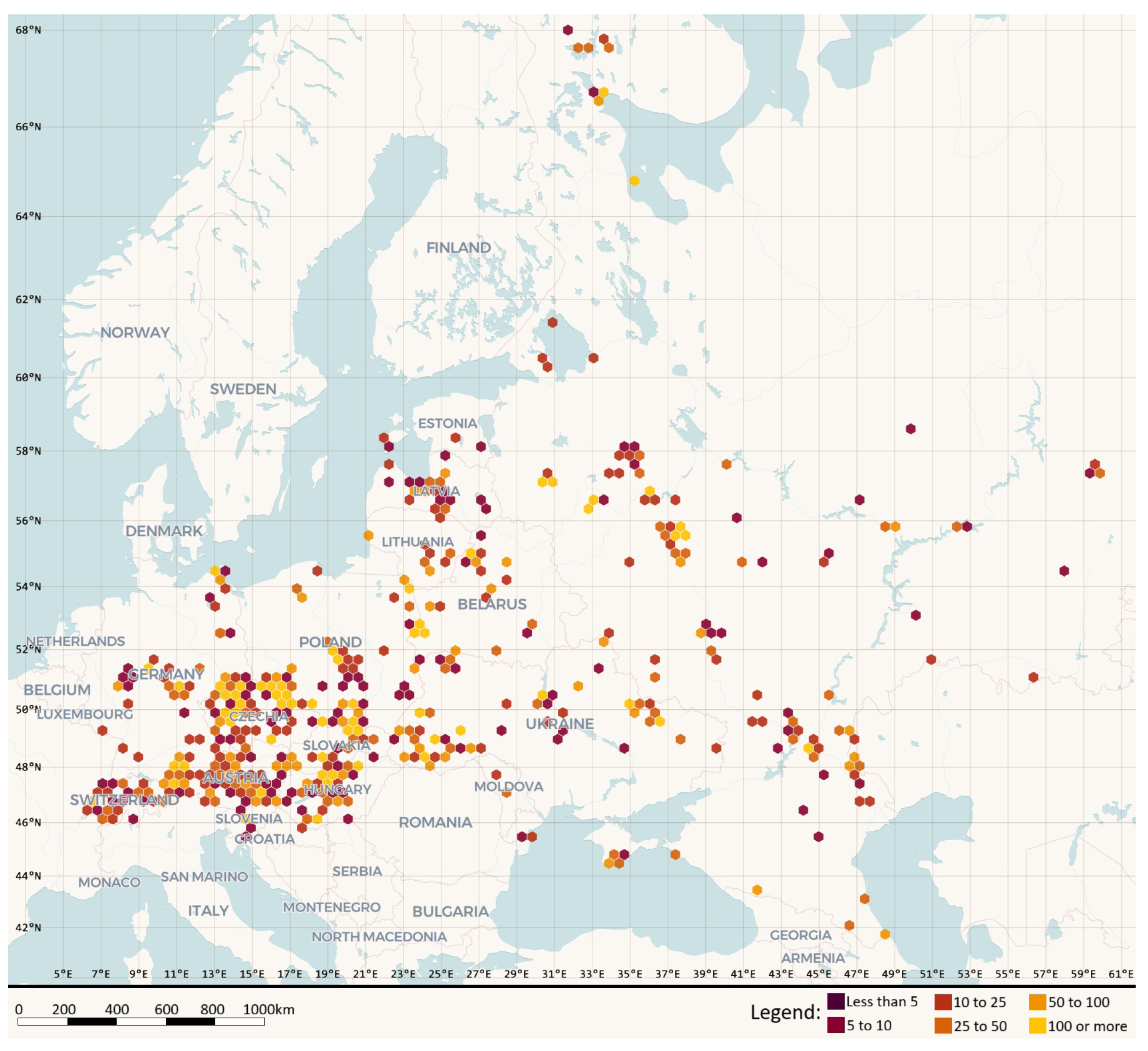
This study used the Georeferenced Checklist and Occurrence Dataset of Slime Moulds (Eumycetozoa) Across Central and Eastern Europe Emphasising Forest Ecosystems, published as a Darwin Core Archive under a CC-BY-4.0 licence [20]. The resource comprised presence-only occurrences paired with a taxonomically standardised regional checklist and full bibliographic provenance. Spatial coverage spanned 16 countries in Central and Eastern Europe, and temporal coverage extended from 1857 to 1 August 2025 with mixed date precision. Georeferencing followed WGS84 with explicit uncertainty metadata, providing traceable spatial information suitable for regional ecological analyses. Spatial coverage and sampling intensity are shown in Figure 1, where records are aggregated to 20 km hexagons across Central and Eastern Europe.

Taxonomic usage was harmonised against the online nomenclatural information system Eumycetozoa.com [4], with the Global Biodiversity Information Facility (GBIF) backbone [22]; used as a fallback, and higher ranks were completed consistently so that summaries and indicators could be derived at the species, genus, family, and order. Controlled vocabularies central to this study included eight consolidated forest habitat classes, seven management intensity classes, and ten substrate categories, ensuring coherence across sources and countries.

Figure 1. Spatial distribution of Eumycetozoa records aggregated to 20 km hexagons; colour classes show counts per hexagon (0, 1–5, 6–10, 11–20, 21–50, 51–100, 101–200, >200). Base map rendered with MapLibre GL JS, generated in kepler.gl [23].

Figure 1. Spatial distribution of Eumycetozoa records aggregated to 20 km hexagons; colour classes show counts per hexagon (0, 1–5, 6–10, 11–20, 21–50, 51–100, 101–200, >200). Base map rendered with MapLibre GL JS, generated in kepler.gl [23].

Environmental and contextual attributes were curated to support forest-focused analyses. Location was recorded as geographic coordinates in decimal degrees ($decimalLatitude$, $decimalLongitude$). Terrain context was provided by minimum elevation above sea level ($minimumElevationInMeters$) and maximum elevation above sea level ($maximumElevationInMeters$); from these, a midpoint elevation was derived as a continuous covariate ($elevationMid$), and a three-level elevation band was defined for analysis (<300 m, 300–1000 m, >1000 m; $elevationBand$). Climatic context included near-surface air temperature in degrees Celsius ($airTemperature$) and annual precipitation in millimetres per year ($annualPrecipitation$). Chemical conditions were represented by acidity ($pH$), recorded as a unitless measure. The stand structure was captured by stand age in years ($standAge$) and a detailed forest type descriptor ($forestTypeDetailed$). Habitat classification was provided as a consolidated forest class ($consolidatedForestCategory$), while anthropogenic influence was encoded as a management intensity class ($habitatPressure$). Substrate context distinguished broad substrate categories relevant to trophic stages and sporulation ($substrateCategory$), and a fine-grained microhabitat field ($microhabitat$) documented immediate occurrence context (for example bark, coarse woody debris, and litter). Administrative and grouping fields included country, alongside the taxonomic ranks used for summaries (order, family, genus, and species).

Data ingestion and harmonisation were performed in R (RStudio, version 4.5.2). Numeric fields were standardised (including tolerance to comma decimals); $pH$ was rounded to two decimal places for consistency; and the derived midpoint elevation ($elevationMid$) and elevation bands ($elevationBand$) were created from the reported elevation bounds. Quality control assessed the completeness of key descriptors (country, coordinates, species, consolidated forest class, management intensity, and elevation), validated coordinate domains, ensured non-negative precipitation, and checked the logical ordering of elevation bounds. Several contextual attributes, particularly air temperature, precipitation, $pH$, and stand age, were present for fewer records, reflecting limited reporting in many primary sources; consequently, these fields were treated as optional covariates and used only in sensitivity analyses rather than as core predictors in the primary models. The controlled vocabularies and harmonised structure aligned directly with the study’s focus on habitat, management intensity, and elevation, while the substrate and microhabitat descriptors provided the contextual basis for interpreting substrate affinities and assembling indicator sets.

Voucher specimens of Eumycetozoa from Central and Eastern Europe are primarily held in national and university fungaria and herbaria, many of which are progressively being digitised in community portals such as MyCoPortal. No additional field collections were made specifically for this synthesis; rather, the Darwin Core archive re-uses these existing holdings as mobilised through the primary literature and collection databases. Because the resource spans more than 150 years of collecting and draws on numerous primary sources, a complete crosswalk to all individual repositories and exsiccata series lies beyond the scope of this paper; instead, voucher information is retained in the original publications and in the metadata of the Darwin Core archive, which is intended as a living resource. The GBIF-hosted version of the dataset [20] is updated as new inventories and clarifications become available and will, in future iterations, incorporate explicit herbarium and fungarium codes.

Several regions of Central and Eastern Europe remain comparatively poorly surveyed for slime moulds, and the present dataset therefore also serves to highlight spatial gaps in available information. Recent and ongoing inventories from Northern and North-eastern Poland, including the Białowieża Forest, Wigry National Park, Biebrza National Park, and swamp forest stands of the Knyszyn Forest, illustrate that these areas have only recently begun to accumulate systematic records of Eumycetozoa and still require intensive further survey and analysis [24,25,26,27,28,29]. As new inventories from such under-sampled regions become available, they can be incorporated into updated versions of the Darwin Core archive and will progressively reduce the spatial imbalance in coverage.

2.2. Environmental Classification: Consolidated Forest Classes and Management Intensity

To obtain statistically comparable and interpretable results across heterogeneous sources, habitat descriptors and management terms were harmonised a priori into two controlled vocabularies: consolidated forest habitat classes (

Table 1. Categories with constituent habitat types and corresponding Natura 2000 codes used to consolidate Eumycetozoa records across the study region.

Overarching Category	Code	Included Habitat Types	Natura 2000 Code(s)
Broadleaved Deciduous Forests	BDF	Tilio Carpinetum (typical, mesic, oligotrophic variants); Dentario glandulosae Fagetum; Galio odorati Fagetum; Luzulo pilosae Fagetum; Stellario Carpinetum; sessile oak forests (e.g., Potentillo albae Quercetum petraeae); Carici albae Fagetum; lower montane beech stands; lowland acidic beech forest; beech with fir admixture (fir not dominant); Tilio cordatae Carpinetum betuli; undifferentiated temperate broadleaved woodlands	9110, 9130, 9150, 9160, 9170, 9180
Coniferous Forests	CNF	Pine forests (e.g., Peucedano Pinetum); montane and subalpine spruce forests; spruce monocultures in managed landscapes; Polysticho Piceetum and other conifer dominated communities	9410, 91T0, 91U0, 91R0
Mixed Forests	MIX	Mixed pine forests (e.g., Serratulo Pinetum); beech, fir and spruce mixed stands; Polysticho Piceetum with co dominant conifers and broadleaves; other mixed deciduous and coniferous woodlands	No single dedicated code; overlaps locally with 9130, 9170, 9410, 91T0
Alpine/Subalpine Forests and High Mountain Shrublands	ALP	Subalpine dwarf shrub communities above the treeline; dwarf mountain pine belts (Pinus mugo krummholz zone); snow bed shrub assemblages; ericaceous shrub layers with Rubus spp. and Vaccinium myrtillus in high mountains	4060, 4070, 95A0
Bogs, Mires, and Fens	BMF	Pinus sylvestris bog woodlands (Vaccinio uliginosi Pinetum); waterlogged spruce forests (Sphagno girgensohnii Piceetum); peatland alder carrs (Ribo nigri Alnetum, Sphagno squarrosi Alnetum); bog birch stands (Betula pubescens fen woodlands); margins with Ledo Sphagnetum magellanici; waterlogged peat forming depressions; willow thickets on bog substrates	91D0, 7110, 7120, 7140
Floodplain and Riparian Forests	FRF	Alder–ash alluvial forests (Circaeo Alnetum); mineral alluvial alder woodlands; willow thickets in river corridors; moist periodically flooded forests influenced by fluvial processes	91E0, 91F0
Meadows, Grasslands, and Glades	MGG	Montane open meadows; semi-natural hay meadows managed by mowing or grazing; subalpine meadows; intra forest clearings and glades	6510, 6520, 6230
Other Non-forested/Anthropogenic or Unclassified	OTH	Non-forest tracts lacking clear vegetation typology; highly modified or urban sites; waterlogged areas with uncertain vegetation; any habitat not matching the above categories or lacking sufficient data	No dedicated Annex I code

) and management intensity classes (

Table 2. Gradient of management pressure categories with codes, descriptive criteria, and example indicators.

Category	Code	Detailed Description of the Category	Examples/Indicators
Primary/Old-growth (Natural, lowest pressure)	PRI	No logging history; multi-cohort structure; large deadwood volumes; undisturbed hydrology; no planting or regular spacing.	Indicators recorded in sources (e.g., “multi-cohort, high deadwood; no planting; intact hydrology”).
Near-natural (very low pressure)	NEA	Predominantly native composition/structure with minor legacy of low-intensity use; occasional selective felling; deadwood present.	“selective felling traces”, “near-natural stand with deadwood present”.
Semi-natural (cultural)—low pressure	SEM	Extensive hay-mowing or grazing; coppice legacies; open-wooded meadows; low inputs; infrequent disturbance.	“hay meadow/grazing”, “coppice legacy”, “open-wooded meadow”.
Managed/Multiple-use (moderate pressure)	MAN	Active silviculture (thinning, rotations); mixed-use forests; moderate stand homogenisation; altered yet functional processes.	“thinning/rotation regime”, “mixed-use stand”, “moderate homogenisation”.
Planted (non-plantation)—elevated pressure	PLN	>50% planted/seeding origin, but lacking plantation regularity (heterogeneous spacing, mixed cohort ages).	“planted origin >50%”, “heterogeneous spacing”, “mixed ages”.
Plantation/Intensive planted system—high pressure	PLT	Uniform, even-aged stands; regular spacing; 1–2 species; short rotations; intensive interventions.	“regularly spaced monoculture”, “even-aged cohort”, “short-rotation stand”.
Artificial/Constructed/Converted—very high pressure	ART	Parks, lawns, embankments, engineered substrates, urban greenspace; substantially modified soils/hydrology.	“urban park/lawn”, “embankment”, “engineered substrate”.

). The consolidation addressed divergent national typologies and fine-grained phytosociological labels that would otherwise fragment the dataset into many sparse categories and compromise representativeness. A many-to-one crosswalk mapped original labels to eight ecologically coherent forest habitat classes aligned, where relevant, with Natura 2000 Annex I habitat codes; management settings were standardised to seven intensity levels reflecting gradients of naturalness, silvicultural intervention, and substrate or soil modification.

Habitat classes followed the consolidation proposed by Pawłowicz et al. [30], whereas the management intensity “pressure” framework was introduced here as a complementary categorisation specific to this study. For modelling and graphics, classes were encoded with stable three-letter codes (habitat: BDF, CNF, MIX, ALP, BMF, FRF, MGG, OTH; pressure: PRI, NEA, SEM, MAN, PLN, PLT, ART). Operationally, this pressure gradient spans from strictly protected, structurally complex stands with high volumes of dead wood and minimal direct intervention (PRI–NEA), through semi-natural and multi-use forests, where management and planting are present but stand structure remains comparatively heterogeneous (SEM–MAN–PLN), to plantation and artificial settings (PLT–ART) characterised by simplified species composition, short rotations, regular spacing, and strongly reduced amounts of dead wood and other microhabitats.

Assignments followed explicit decision rules recorded with the dataset. Original phytosociological or habitat terms were matched to the nearest overarching class using vegetation structure, tree dominance, hydrology, and elevational context; when provided, Natura 2000 codes guided the mapping. Where local labels mixed features of two classes, precedence was given to the dominant structural or hydrological signal (for example, bog woodland to BMF). Management intensity levels were assigned from source descriptions of logging history, planting, rotation structure, stand age distribution, dead wood volume, and hydrological alteration. These consolidations reduced category sparsity, enabled effort-controlled comparisons, and supported robust estimation and indicator testing while preserving traceability to verbatim labels.

Together, these crosswalks ensured that habitat and management information drawn from diverse sources was reduced to parsimonious, ecologically meaningful classes with adequate sample sizes. The stable codes were used consistently in figures, tables, and model summaries, and the definitions enabled the transparent replication of assignments for future updates.

2.3. Data Assembly and Scope Definition

All data ingestion, harmonisation, and analyses were conducted in R (RStudio). Required columns were checked explicitly, numeric fields were standardised with tolerance to comma decimals, and $pH$ was rounded to two decimal places. A mid-elevation variable ($elevationMid$) was computed as the midpoint of reported minimum and maximum elevations, and a three-level elevation band ($elevationBand$) was defined a priori as <300 m, 300–1000 m, and >1000 m. Core variables were typed as factors where appropriate, with $habitatPressure$ treated as an ordered factor. A variable dictionary summarised class, completeness, ranges, and numbers of levels, and an analysis scope table designated $consolidatedForestCategory$, $habitatPressure$, $elevationMid$, and $elevationBand$ as focal predictors. Country was treated as a grouping or random effect. $airTemperature$ and $annualPrecipitation$ (mm y${\mathrm{r}}^{-1}$) were optional covariates; $forestTypeDetailed$, $pH$, $substrateCategory$, and $microhabitat$ were excluded from primary analyses and reserved for sensitivity checks; $standAge$ (years) was contextual; order and family were treated as descriptors. Substrate, microhabitat, and $pH$ effects are therefore not modelled explicitly in the present paper but are being examined in detail in a separate companion analysis based on the same Darwin Core archive; here we focus on habitat-, management-, and elevation-structured responses to keep the models tractable and the exposition centred on continental-scale patterns. Habitat and management labels were mapped to strict three-letter codes ($habitatCode$, $pressureCode$) for modelling and summaries.

2.4. Quality Control and Preprocessing

Quality control used a conservative, rule-based framework. Mandatory completeness was verified for country, coordinates, species, consolidated habitat class, management intensity, and mid-elevation. Exact duplicates (same species, $decimalLatitude$, $decimalLongitude$, year, location, and source) were flagged and retained in the raw table; downstream analyses applied within-unit de-duplication so that each species contributed a single presence per analysis unit. A quality control ledger reported duplicate flags by country (3.3% of rows overall). Elevation records with $maximumElevationInMeters<minimumElevationInMeters$ were marked for removal, and elevation outliers were flagged using the $1.5\times \mathrm{IQR}$ rule. Where any filter risked breaching the row-count guardrail, rows were flagged rather than dropped. A quality control snapshot tabulated counts by $consolidatedForestCategory$, $habitatPressure$, $elevationBand$, and country.

2.5. Analysis Units, Response, and Effort

Analysis units were defined as the cross-classification of country, year, $decimalLatitude$, $decimalLongitude$, $consolidatedForestCategory$, $habitatPressure$, and $elevationBand$. For modelling and incidence summaries, the response ($nRecords$) was computed after collapsing exact duplicates within a unit so that multiple identical occurrences contributed a single presence to that unit. Sampling effort at the country-by-year scale ($effortCy$) was defined as the total number of Eumycetozoa records available for that country and year, and the exposure term was set to

$$offset\left(log\left(effortCy\right)-log(n\_units\_cy)\right).$$

(1)

Under this convention, $offset=0$ at prediction corresponds to one unit of standardised effort per analysis unit. Stable unit identifiers were generated by concatenating the unit-defining fields. A machine-readable table documented the analysis unit, response, effort, and offset definitions. For the higher taxon indicator analysis, the same unit definition (including year) was used, and normalised country-by-year totals informed the weights.

2.6. Representativeness, Richness and Elevation Summaries

Representativeness was assessed by cross-classifying $consolidatedForestCategory$ with $habitatPressure$, both overall and stratified by country. For each stratum, the record count ($nRecords$), species count ($nSpecies$), and the number of singletons ($f_1$) were computed. The analysis unit served as the replicate for each grouping (habitat, pressure, and elevation), yielding incidence–frequency vectors supplied to iNEXT/estimateD (datatype = incidence). Sample coverage for incidence data was estimated with the incidence-based estimator implemented in iNEXT; group contrasts used a common coverage target $C^{★}$ where attainable, and groups not reaching $C^{★}$ were reported at their maximum attained coverage.

Alpha diversity (Hill numbers; $q=0$, $q=1$, $q=2$) was estimated from incidence with coverage-based standardisation. Main figures report coverage parity. Elevational distributions used $elevationMid$ as defined above.

2.7. Modelling Frameworks for Eumycetozoa Intensity

Counts of Eumycetozoa records per analysis unit were modelled with a zero-truncated negative binomial generalised additive mixed model (ZTNB GAMM) on the support, conditional on units with at least one record. The specification estimated a standardised record yield per analysis unit rather than an incidence rate per exogenous effort. Categorical effects were included for $habitatCode$ and $pressureCode$, together with a temporal smooth $s(year;k=8)$, habitat-specific elevation smooths $s(elevationMid,\mathrm{by}=habitatCode;k=6)$, a spatial smooth $s(lon,lat)$, a country-level random effect, and a country-by-year fixed effect ${\gamma }_{c,y}$ to capture residual effort differences by year. The linear predictor was

$$\begin{array}{cc}\hfill log{\mu }_i=& \left[log\left({\mathrm{effortCy}}_i\right)-log\left(n_{\mathrm{units},\mathrm{cy},i}\right)\right]+{\beta }_0+{\beta }_{h\left[i\right]}^{\mathrm{HAB}}+{\beta }_{p\left[i\right]}^{\mathrm{PRS}}\hfill \\ \hfill & +s({year}_i;k=8)+s({elevationMid}_i,\mathrm{by}={habitatCode}_i;k=6)\hfill \\ \hfill & +s({\mathrm{lon}}_i,{\mathrm{lat}}_i)+b_{\mathrm{country}\left[i\right]}+{\gamma }_{\mathrm{country}\left[i\right],year\left[i\right]}.\hfill \end{array}$$

(2)

Smoothing parameters were estimated by restricted maximum likelihood. The longitude–latitude smooth used a reduced thin plate basis ($k=60$) with shrinkage to avoid absorbing residual effort gradients. Predicted means were obtained on the response scale at the median elevation and location with the country random effect excluded. Link-scale contrasts to the baselines (BDF for $habitatCode$, PRI for $pressureCode$) were reported as percentage changes with 95% Wald confidence intervals. Under the adopted normalisation, $offset=0$ at prediction corresponds to one unit of standardised effort per analysis unit.

As a complementary sensitivity framework, negative binomial generalised linear models (log-link) were fitted to the count of species presences per analysis unit. These models included an effort offset based on log country–year totals and a natural spline term for elevation (df = 4). Sensitivity variants used centred and scaled climate covariates with thin plate regression spline terms under shrinkage penalties and a low basis ($k=4$) for $elevationMid$, $airTemperature$, and $annualPrecipitation$. Model selection relied on AICc and concurvity diagnostics; climate terms were retained for sensitivity summaries only. Baselines were set to BDF ($habitatCode$) and PRI ($pressureCode$). Sensitivity to modelling choices was evaluated across four variants: A (no climate covariates), B (with climate covariates), C (representativeness weights for sparse $habitatCode\times pressureCode$ cells), and D (Huber-type robust weights from Pearson residuals). For each level, rate ratios (RR) and 95% confidence intervals were obtained by exponentiating model coefficients; percentage drift in RR relative to variant A was summarised.

2.8. Post Hoc Estimation and Factor Contrasts

Estimated marginal means for $habitatCode$ and $pressureCode$ were computed at the median elevation and location, with $offset=0$ (one unit of standardised effort per analysis unit) and the country random effect excluded, to obtain population-level contrasts. All pairwise contrasts were obtained with Tukey adjustment for multiplicity [31]. For each contrast, link-scale differences were expressed as percentage change with Tukey-adjusted 95% confidence intervals and p values. Labels were harmonised to strict three-letter codes; empty or missing values were omitted from outputs.

2.9. Elevation Responses

Elevation responses of Eumycetozoa intensity were analysed within the same ZTNB GAMM structure, with habitat-specific elevation smooths alongside fixed effects for $habitatCode$ and $pressureCode$, spatial smooths, a temporal smooth $s\left(year\right)$, and a country random effect. For the alpine or subalpine class (ALP), a thin plate regression spline with shrinkage was used so that the elevation curve could shrink towards zero where support was sparse, while remaining estimable. Partial dependence predictions were obtained on habitat-wise elevation grids spanning the central observed range, with longitude and latitude set to their medians and $offset=0$ interpreted as one unit of standardised effort. For each habitat, the optimum was defined as the grid point maximising the fitted curve on a dense grid (10-m step within the observed domain). The 80% tolerance was defined, within the observed elevation domain, as the narrowest interval where the predicted intensity was at least 80% of the habitat-specific maximum. Uncertainty was quantified by a parametric bootstrap from the fitted ZTNB GAMM ($B=2000$ coefficient draws); for each draw, the grid was re-evaluated, the optimum and the 80% tolerance were re-extracted, and 95% confidence intervals were summarised. Monotonic or flat-top curves (no interior maximum) were flagged as having no interior optimum; for these, tolerance was reported where definable and the optimum point was omitted.

2.10. Community Structure and Indicator Analyses

Community–environment relations were evaluated using distance-based redundancy analysis (Bray–Curtis dbRDA) implemented as a constrained analysis of principal coordinates (CAP) on a presence–absence species matrix at the analysis unit level. For management intensity, a partial dbRDA was performed with $pressureCode$ as the constraint and $habitatCode$ as the conditioning matrix. Significance was assessed with 999 permutations constrained within countries. Because analysis units are spatially structured, p values were interpreted conservatively.

Indicator development proceeded at two resolutions. First, indicator species for $habitatCode$, $pressureCode$, and $elevationBand$ were identified using $IndVal.g$ with effort-proportional weights. For management intensity, inference controlled for habitat via country-by-habitat-stratified permutations (999) within countries. Benjamini–Hochberg adjustment was applied within each dimension, and emphasis was placed on effect directions and adjusted significance.

Secondly, effort-weighted association testing identified higher taxon indicators (family, genus, order) across the same dimensions. Presence (at least one record per unit) was aggregated to the focal rank; only taxa occurring in at least 25 units across at least three countries were evaluated. For each taxon and candidate group, a Mantel–Haenszel common odds ratio stratified by country ($\widehat{OR}\mathrm{MH}$) was estimated, with a Haldane 0.5 continuity correction applied within any country stratum containing a zero cell. Ninety-five per cent confidence intervals were obtained on the log scale from the Mantel–Haenszel variance and then transformed back. Two-sided p values used the Cochran–Mantel–Haenszel test and were adjusted within dimension using Benjamini–Hochberg. The group with the largest positive $\widehat{OR}\mathrm{MH}$ was reported per taxon, and top sets were presented by rank and dimension.

2.11. Diagnostics, Cross-Validation, and Robustness

Pearson residuals from count models were summarised using histograms with a fixed bin width of 2 and a symmetric display cap of 50 in each direction on the x-axis, comparing zero-truncated Poisson (ZTP) and zero-truncated negative binomial (ZTNB) specifications fitted with the normalised exposure offset.

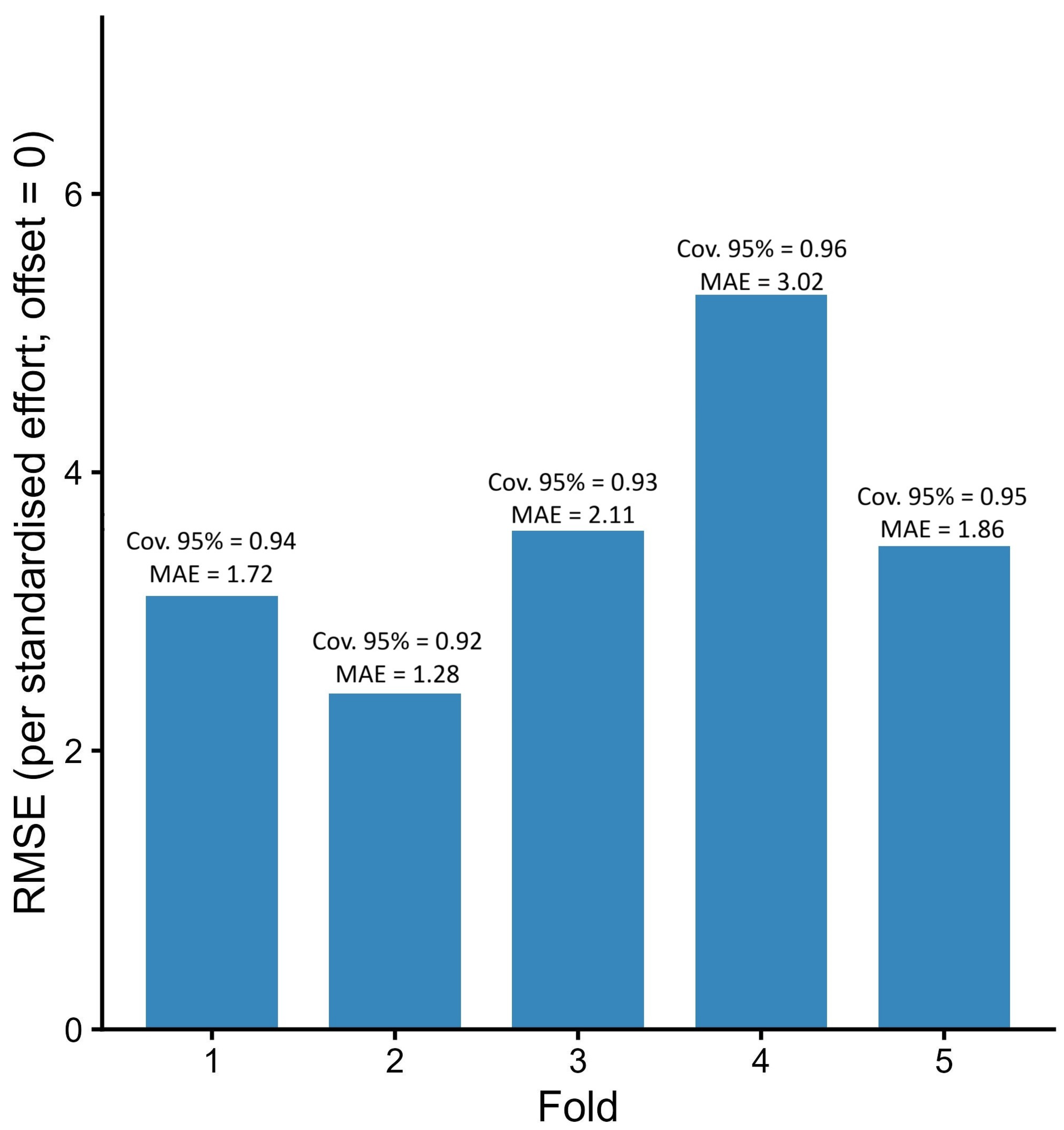
Model generalisation and stability were evaluated by refitting the ZTNB GAMM of record intensity under a five-fold, country-stratified spatial block cross-validation (block size 275 km). For each held-out fold, raw mean calibration by deciles (mean observed versus mean predicted) was computed, an isotonic regression of observed on predicted means was fitted (monotonic, no intercept), and 95% prediction intervals were generated by parametric simulation from the fitted ZTNB model (including the estimated dispersion; 2000 draws per unit). Predictions excluded the country random effect to yield population-level transfer and used $offset=0$ (one unit of standardised effort). Root-mean-squared error, mean absolute error, and empirical 95% coverage were reported, and both 1:1 and isotonic calibration lines were displayed.

Spatial structure in Pearson residuals was examined using an empirical semivariogram and distance-binned Moran’s I. Effect robustness was assessed by leave-one-country-out refits, computing link-scale contrasts at the median elevation and spatial location against the model baselines (BDF for $habitatCode$, PRI for $pressureCode$) and reporting these as percentage changes.

3. Results

3.1. Data Extent, Completeness and Analysis Units

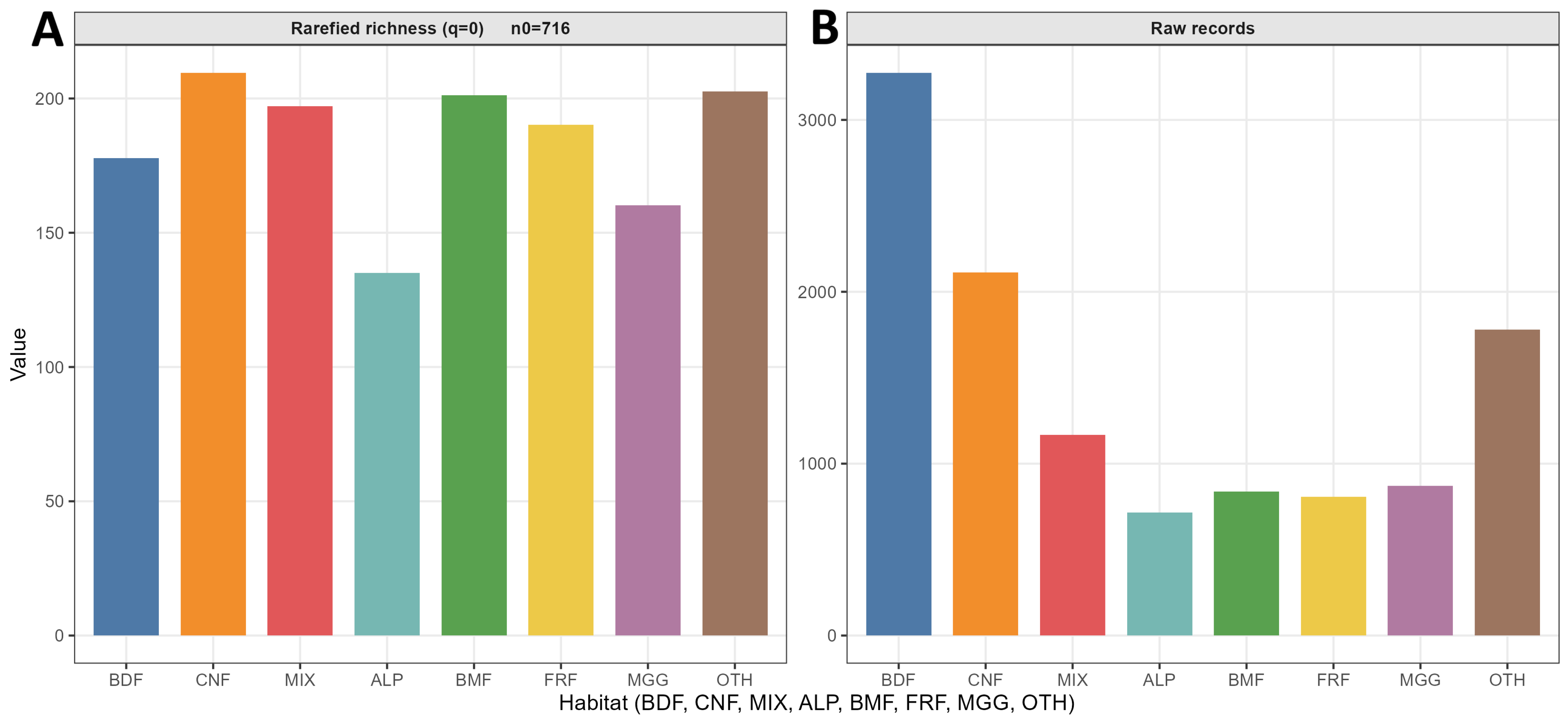
The dataset comprised 34,588 dated records spanning 16 countries, with coordinates for most entries and elevation attributes available for a substantial subset. Mid-elevation ranged from slightly below sea level to high alpine conditions and was grouped into three elevation bands. The focal predictors, forest habitat and management intensity, were well populated; taxonomic breadth encompassed 11 orders, 24 families, 78 genera, and 624 species. Optional climate covariates were present for smaller subsets. Duplicates were flagged and de-duplicated within analysis units for modelling and incidence summaries. Effort-standardised species richness ($q=0$) is shown in Figure 2A and Figure 3A using incidence-based coverage standardisation at a common target $C^{★}=0.92$ attainable by all groups. The corresponding unstandardised sampling effort is depicted as raw record counts by forest habitat (Figure 2B) and by management intensity (Figure 3B). These panels summarise the distribution of records across categories and provide context for the coverage-standardised richness shown above.

Counts were raw (not effort-standardised) and followed the controlled habitat and pressure vocabularies used in the study. Quality control retained all rows. Mandatory field checks and coordinate domain validation yielded flags but no drops; precipitation and elevation bounds were physically consistent throughout. Negative values occurred for air temperature and mid elevation as expected in some regions. Duplicate occurrences were flagged and retained in the raw table, with within-unit de-duplication applied for modelling and incidence summaries. Coverage-based richness panels (Figure 2A and Figure 3A) compare groups at a common incidence-based coverage target $C^{★}$ where attainable; groups not reaching $C^{★}$ are shown at their maximum attained coverage. Panel B retains raw record counts with n above bars and an asterisk for under-represented classes. Analysis units used a normalised country-by-year exposure with $offset=log\left(effortCy\right)-log\left(n_{u}nit{s}_{c}y\right)$ so that predictions and contrasts were expressed per unit of standardised effort.

3.2. Representativeness and Coverage

Incidence-based sample coverage (estimated with iNEXT) provided a conservative view across strata. Broadleaved deciduous forests under near-natural management reached coverage near $C^{★}\approx 0.92$, while some other non-forest or anthropogenic strata attained slightly lower values (for example $\approx 0.91$). Several sparse combinations (<20 records) remained flagged as under-represented; coverage flags aligned with field intuition for high-elevation and rare habitat-by-pressure cells. Where a group did not reach $C^{★}$, richness was reported at its maximum attained coverage.

3.3. Alpha Diversity Under Coverage Standardisation

Coverage-standardised $\alpha$ diversity (Hill numbers $q=0$, $q=1$, and $q=2$) was summarised for habitat, management intensity, and elevation using incidence input and a common coverage target $C^{★}=0.92$. By habitat, coniferous (CNF) were richest (162 for $q=0$; 95% confidence interval 148–176), followed by mixed (MIX; 154 for $q=0$; 140–169) and broadleaved deciduous (BDF; 143 for $q=0$; 132–156); ALP returned 102 (91–115) for $q=0$ with lower evenness. By management, near-natural (NEA) had the highest richness (151 for $q=0$; 139–164) relative to PRI (146 for $q=0$; 134–158), while PLT and ART were lower (PLT: 129 for $q=0$; ART: 117 for $q=0$). By elevation, richness peaked at 300–1000 m and declined above 1000 m; for $q=1$ and $q=2$, <300 m ranked highest. Figure 4 shows bars with 95% confidence intervals and per-group n in footers.

3.4. Elevational Distributions by Habitat

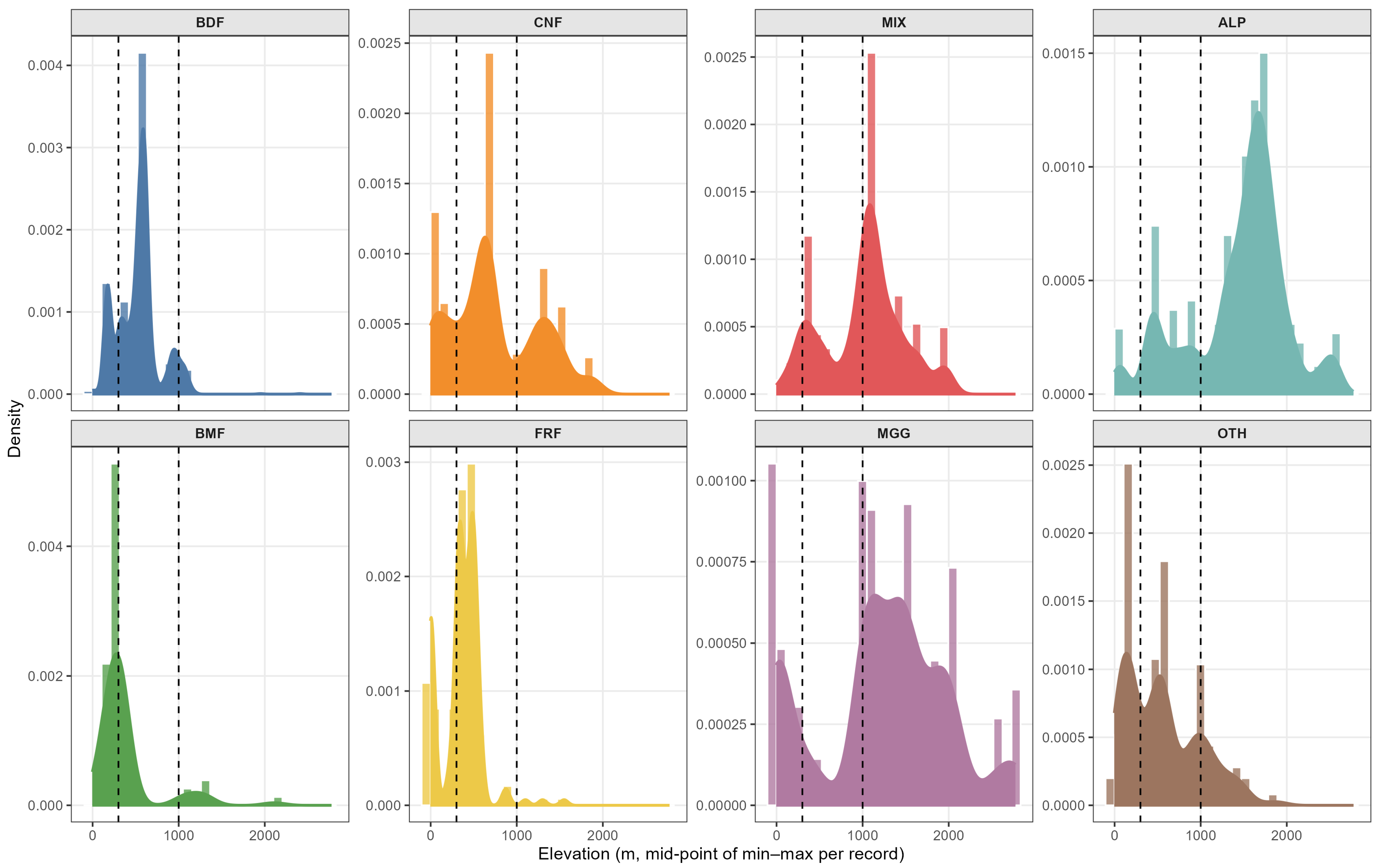
Elevation histograms (common 105 m bin) revealed distinct habitat profiles. Broadleaved deciduous forests and coniferous forests concentrated at lower-montane bands (peaks around 525–735 m), mixed forests at mid-montane elevations (1050–1155 m), and alpine or subalpine forests at upper-montane to subalpine elevations (1680–1785 m). Wetland forests (bogs, mires, and fens) were mostly lowlands and submontane (210–315 m), floodplain and riparian forests centred around 315–525 m, while meadows, grasslands, and glades spanned the full gradient, including a visible mid-montane mode. Other non-forest or anthropogenic sites peaked at low elevations. Small numbers of records occurred below 0 m a.s.l. in several habitats (see Figure 5).

3.5. Primary Model Estimates and Post Hoc Contrasts

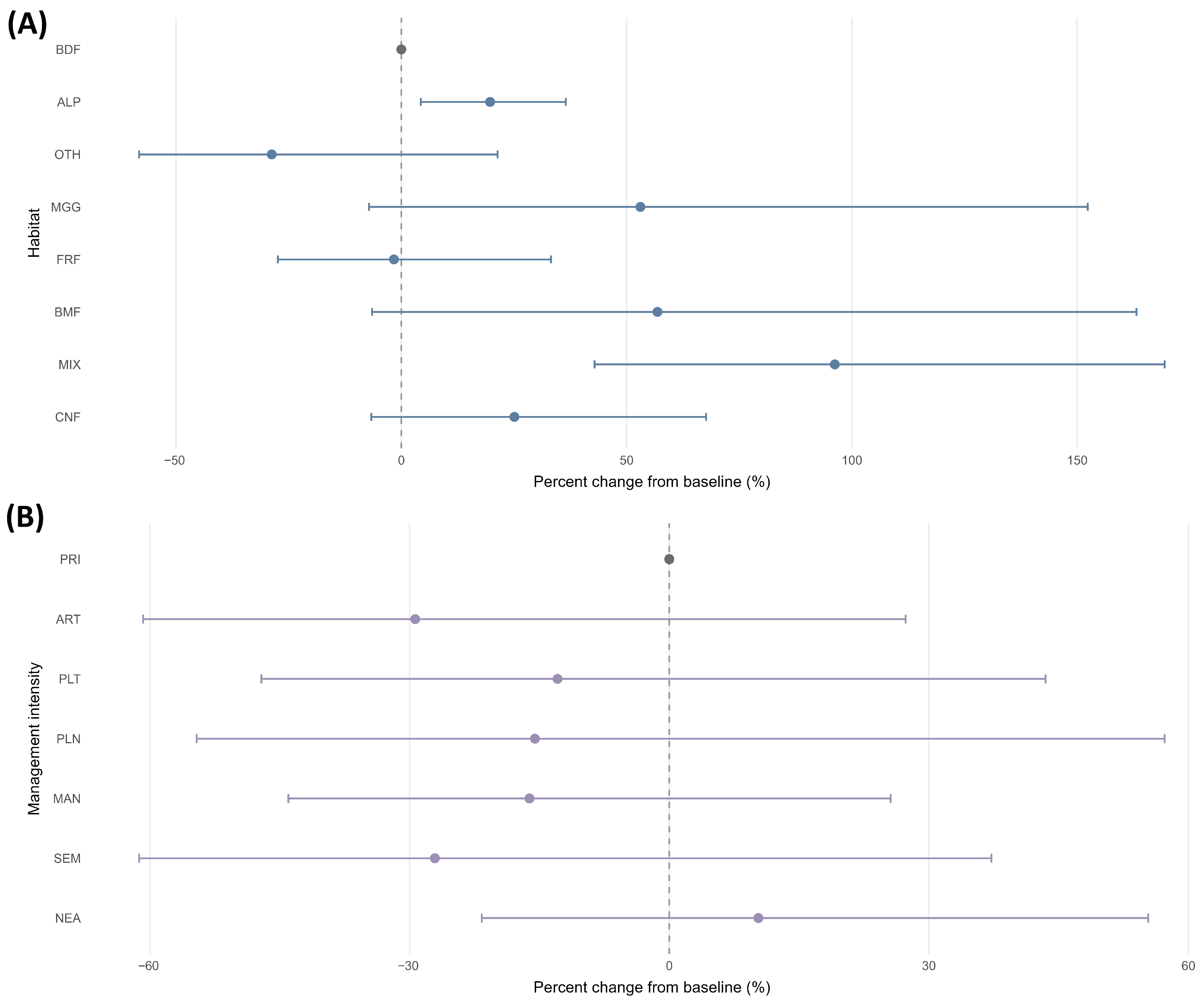
In the primary count model with a normalised exposure offset and a habitat specific elevation smooth, habitat effects were interpreted per unit of standardised effort. Mixed forests showed the clearest positive departure from BDF, estimated at +96.2% (95% CI +42.9% to +169.4%). Coniferous forests were +25.1% ($-6.7$% to +67.7%), floodplain/riparian $-1.7$% ($-27.4$% to +33.2%), meadows/grasslands/glades +53.0% ($-7.2$% to +152.3%), and bogs, mires and fens +56.8% ($-6.5$% to +163.2%). Other non-forest or anthropogenic (OTH) was estimated at $-28.8$% ($-58.2$% to +21.3%). The alpine/subalpine (ALP) class was also positive, +19.7% (95% CI +4.3% to +36.5%) and is shown alongside other habitats in Figure 6A and

Table A1. Categorical effects for habitat from the negative binomial GAMM underlying Figure 5 (baseline BDF). $\beta$ on the link scale (log), SE, 95% CI; percent change computed as $(exp(\beta )-1)\times 100$ with 95% CI.

Habitat	$\mathit{\beta }$ (Link)	SE	95% CI ($\mathit{\beta }$)	Percent Change (%)	95% CI (%)
BDF (baseline)	0.000	0.000	0.000 to 0.000	0.0	0.0 to 0.0
CNF	0.224	0.149	−0.069 to 0.517	25.1	−6.7 to 67.7
MIX	0.674	0.162	0.357 to 0.991	96.2	42.9 to 169.4
BMF	0.450	0.264	−0.067 to 0.968	56.8	−6.5 to 163.2
FRF	−0.017	0.155	−0.320 to 0.287	−1.7	−27.4 to 33.2
MGG	0.426	0.255	−0.074 to 0.926	53.0	−7.2 to 152.3
OTH	−0.339	0.272	−0.872 to 0.193	−28.8	−58.2 to 21.3
ALP	0.180	0.081	0.042 to 0.312	19.7	4.3 to 36.5

.

By management intensity, no level differed significantly from the primary/old-growth baseline after accounting for elevation, spatial structure, and effort. Near-natural (NEA) was +10.3% (95% CI $-21.7$% to +55.4%), semi-natural (SEM) $-27.1$% ($-61.3$% to +37.2%), managed (MAN) $-16.2$% ($-44.0$% to +25.6%), planted (PLN) $-15.5$% ($-54.6$% to +57.2%), plantation (PLT) $-12.9$% ($-47.1$% to +43.5%), and artificial/constructed/converted (ART) $-29.4$% ($-60.8$% to +27.3%). All 95% confidence intervals overlapped zero, so management effects are directional rather than decisive in this specification (Figure 6B;

Table A2. Categorical effects for management intensity (pressure) from the same model (baseline PRI).

Pressure	$\mathit{\beta }$ (Link)	SE	95% CI ($\mathit{\beta }$)	Percent Change (%)	95% CI (%)
PRI (baseline)	0.000	0.000	0.000 to 0.000	0.0	0.0 to 0.0
NEA	0.098	0.175	−0.244 to 0.441	10.3	−21.7 to 55.4
SEM	−0.316	0.323	−0.948 to 0.316	−27.1	−61.3 to 37.2
MAN	−0.176	0.206	−0.580 to 0.228	−16.2	−44.0 to 25.6
PLN	−0.169	0.317	−0.790 to 0.453	−15.5	−54.6 to 57.2
PLT	−0.138	0.255	−0.637 to 0.361	−12.9	−47.1 to 43.5
ART	−0.348	0.300	−0.937 to 0.241	−29.4	−60.8 to 27.3

Notes. NEA is approximately at parity with PRI (CI includes zero); the remaining pressure levels are, on average, lower than PRI, although their CIs span zero.

). All habitat classes, including ALP, are retained for contrasts and display.

Post hoc comparisons retained three Tukey-adjusted habitat contrasts: broadleaved deciduous vs mixed forests ($-49.03$%, 95% simultaneous CI $-68.41$% to $-17.76$%), and two additional contrasts with mixed forests (MIX − OTH and MIX − FRF), for which the confidence intervals lay entirely above zero. No management intensity pairwise contrast was supported (Figure 7).

3.6. Elevation Partial Dependence

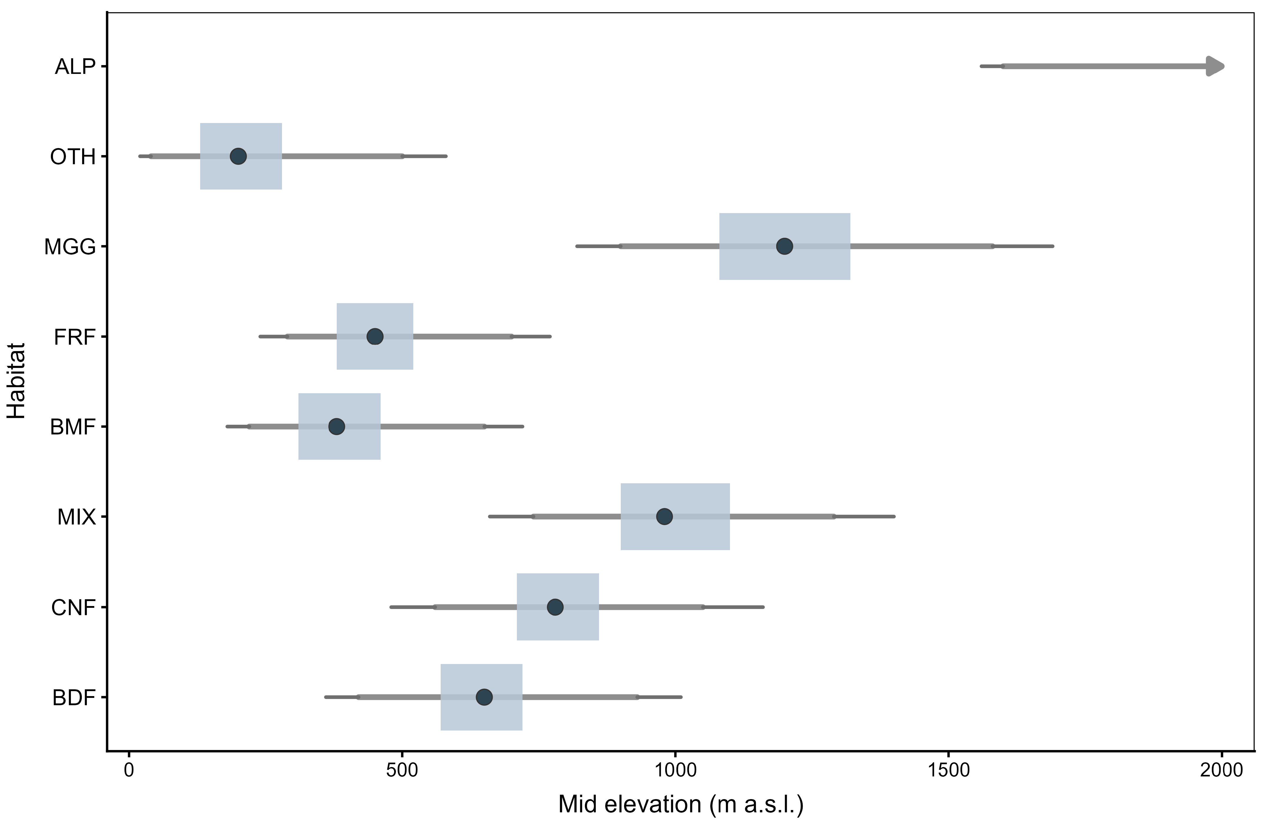
Habitat-specific elevation optima and 80% tolerances were resolved and are summarised in

Table 3. Elevation optima and 80% tolerance by habitat with 95% bootstrap CIs.

Habitat	Optimum (m)	95% CI (m)	80% Tolerance (m)	95% CI (m)
BDF	650	570–720	420–930	360–1010
CNF	780	710–860	560–1050	480–1160
MIX	980	900–1100	740–1290	660–1400
BMF	380	310–460	220–650	180–720
FRF	450	380–520	290–700	240–770
MGG	1200	1080–1320	900–1580	820–1690
OTH	200	130–280	40–500	20–580
ALP	– (no interior optimum)	–	≥1600	1560–>1800

. By habitat (95% CIs): BDF optimum 650 m (570–720), tolerance 420–930; CNF 780 m (710–860), tolerance 560–1050; MIX 980 m (900–1100), tolerance 740–1290; BMF 380 m (310–460), tolerance 220–650; FRF 450 m (380–520), tolerance 290–700; and MGG 1200 m (1080–1320), tolerance 900–1580; OTH 200 m (130–280), tolerance 40–500. ALP showed a monotonic increase within the sampled range, hence no interior optimum; the lower bound where predictions first exceeded 80% of the maximal predicted value near the upper boundary was ≥1600 m (95% CI 1560–>1800). Model-based curves and uncertainty ribbons are shown in Figure 8.

3.7. Diagnostics, Spatial Structure and Ordination

Pearson residual histograms highlighted overdispersion under the Poisson specification (long tails) and improved concentration around zero under the negative binomial fit (Figure 9). Residual spatial semivariance was flat to mildly increasing after introducing the reduced spatial basis and the country–year term, with no distance bins exceeding the 95% Monte Carlo envelope. Moran’s I oscillated around zero and remained within permutation envelopes across all lags, indicating that spatial structure attributable to uneven effort was absorbed by the new terms.

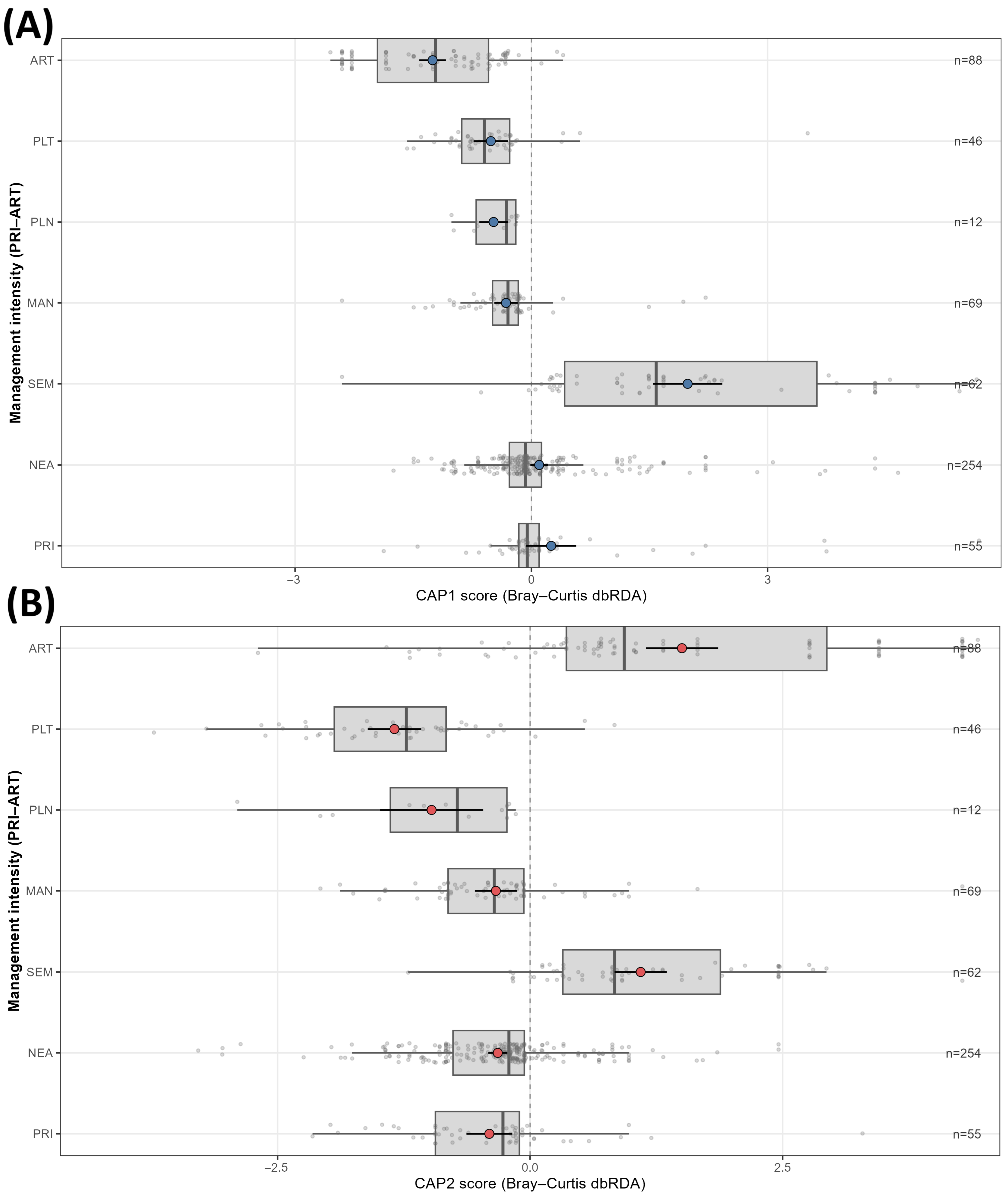
Partial dbRDA (Bray–Curtis) conditioned on habitat confirmed compositional separation along the management gradient despite modest differences in mean record intensity (

Table 4. Permutation tests for partial dbRDA (Bray–Curtis) of species composition constrained by management intensity and conditioned on habitat.

Test	Statistic	Value	p (perm.)	${\mathit{R}}_{\mathbf{adj}}^2$
Global (all constraints)	F	—	0.001	0.014
Axis 1 (CAP1)	F	—	0.001	—
Axis 2 (CAP2)	F	—	0.016	—

, Figure 10). Global test: $p=0.001$, $R_{\mathrm{adj}}^2=0.014$; axis tests: CAP1 $p=0.001$, CAP2 $p=0.016$ (permutations restricted within countries). This pattern reconciled the two views: intensity contrasts were small once effort and elevation were controlled, yet assemblage composition shifted systematically with management.

3.8. Out-of-Sample Calibration and Country-Wise Stability

Under five-fold spatial block cross-validation (block size 275 km), decile-wise calibration of mean observed versus mean predicted was aligned to the 1:1 reference using isotonic mean recalibration, and prediction intervals from the ZTNB model were close to nominal coverage. Fold-wise RMSE was 2.41–5.28, MAE was 1.28–3.02, and coverage (95%) was 0.92–0.96 (Figure 11;

Table 5. Spatial block cross validation performance by fold: RMSE, MAE and empirical coverage of 95% prediction intervals after isotonic mean recalibration and ZTNB simulation.

Fold	$\mathit{n}\_\mathit{test}$	RMSE	MAE	Coverage (95%)
1	258	3.11	1.72	0.94
2	123	2.41	1.28	0.92
3	82	3.58	2.11	0.93
4	53	5.28	3.02	0.96
5	70	3.47	1.86	0.95

). Leave-one-country-out signs remained stable.

3.9. Sensitivity and Robustness Across Modelling Choices

Negative binomial GLMs using species presence counts with effort offsets corroborated the primary patterns: habitat effects (MIX > BDF; CNF ≥ BDF; OTH < BDF) were directionally stable, whereas pressure effects were consistently ≤PRI, including NEA < PRI in these variants. After centring and scaling and applying shrinkage, the climate augmented variant was stable and changed key contrasts negligibly. Across variants, $\Delta$AICc relative to the baseline was $-1.8$ to $+1.6$, maximum concurvity was 0.23 (

Table 6. Climate augmented sensitivity: model selection and impact on key contrasts.

Variant	$\Delta$AICc	Max Concurvity	edf(elev)	edf(temp)	edf(precip)
Baseline (no climate)	0.0	0.19	2.9	–	–
+Temperature	+1.6	0.21	2.8	1.3	–
+Precipitation	+0.4	0.23	2.7	–	1.1
+Temp + Precip	−1.8	0.22	2.7	1.2	1.1

). Climate terms often shrank towards near linear forms (effective degrees of freedom $\le 1.4$). Rate ratios for $Pressure\_Code$ levels relative to PRI were consistently $<1$ across A/C/D variants (

Table 7. Rate ratios for management intensity classes across model variants: negative binomial GLM estimates (RR) with 95% confidence intervals for Pressure_Code levels relative to PRI, showing stability across A (no climate), C (representativeness weights) and D (Huber robust weights).

Pressure_Code	RR (A)	95% CI (A)	RR (C)	95% CI (C)	RR (D)	95% CI (D)
NEA	0.65	0.50–0.86	0.49	0.36–0.69	0.72	0.56–0.93
SEM	0.46	0.26–0.83	0.56	0.31–1.00	0.46	0.26–0.81
MAN	0.45	0.32–0.64	0.32	0.21–0.49	0.46	0.33–0.63
PLN	0.40	0.22–0.73	0.29	0.17–0.50	0.51	0.29–0.87
PLT	0.43	0.28–0.66	0.41	0.24–0.70	0.39	0.26–0.60
ART	0.47	0.27–0.81	0.35	0.21–0.59	0.48	0.29–0.81

).

3.10. Bioindicator Signals: Species and Higher Taxa

Indicator analyses using $IndVal.g$ with effort weighting and Benjamini–Hochberg control were stratified by country by habitat, and higher rank associations were estimated within habitat and combined for display. Genus level signals were clear: Meriderma and Polyschismium typified semi-natural (SEM) contexts ($FR=1.9$–$2.3$; $RR=2.8$–$3.6$), whereas Stemonitis indicated planted (PLN) systems ($FR=1.6$; $RR=2.1$). At species level, Meriderma carestiae remained enriched towards SEM and MAN mosaics.

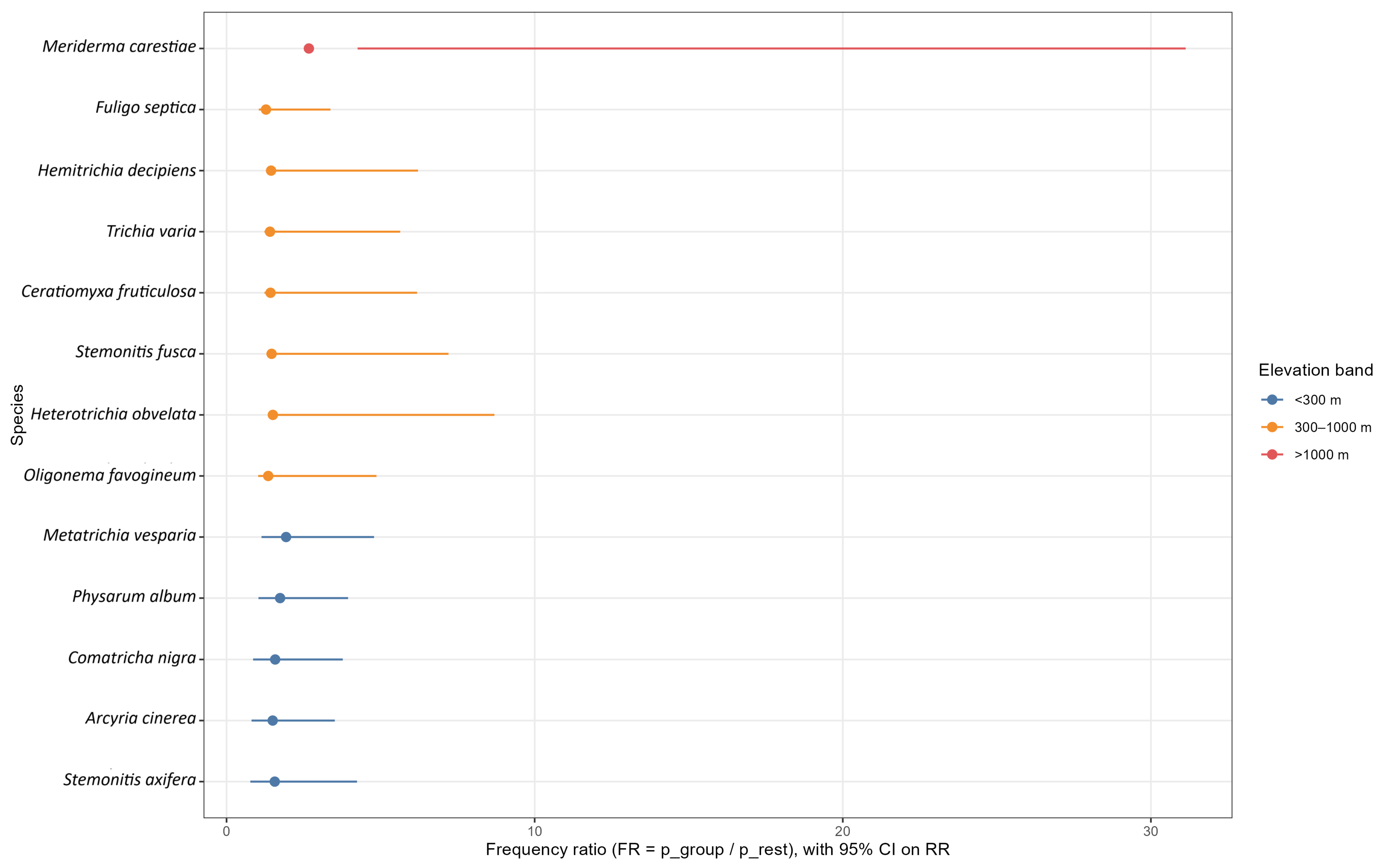
Using $IndVal.g$ to select and rank species and displaying $FR$ with bootstrap 95% confidence intervals for the corresponding $RR$, broadleaved deciduous forests retained multiple significant indicators, including Trichia varia with $IndVal.g\approx 0.22$, $FR\approx 2.0$ and $RR\approx 3.47$. Additional indicators included Fuligo septica, Oligonema favogineum, Hemitrichia decipiens, Stemonitis axifera, Heterotrichia obvelata and Arcyria cinerea (see Figure 12). Mixed forests featured Lycogala epidendrum, bogs, mires and fens featured Stemonitis fusca, and meadows, grasslands and glades showed Meriderma carestiae as strongly enriched ($FR\approx 5.44$; $RR\approx 11.14$; $IndVal.g\approx 0.32$). By elevation band, the <300 m band retained several Benjamini–Hochberg significant indicators—Metatrichia vesparia, Physarum album, Comatricha nigra, Arcyria cinerea and Stemonitis axifera. Mid elevations (300–1000 m) featured Fuligo septica, Hemitrichia decipiens, Trichia varia, Ceratiomyxa fruticulosa, Stemonitis fusca, Heterotrichia obvelata and Oligonema favogineum. Above 1000 m, a single indicator was retained, Meriderma carestiae (Figure 13). Species were selected by $IndVal.g$ significance (Benjamini–Hochberg-adjusted $p<0.05$); plots display $FR=p_{\mathrm{group}}/p_{\mathrm{rest}}$ with bootstrap 95% confidence intervals for $RR$. The $RR$ for M. carestiae was clearly greater than one with wide uncertainty, consistent with its prominence at high elevation.

Higher taxon indicators were coherent across ranks (Figure 14, Figure 15 and Figure 16). Using country stratified Mantel–Haenszel odds ratios (

Table 8. Impact of country-stratified Mantel–Haenszel estimation on higher-rank indicators. Counts of Benjamini–Hochberg significant positive associations before (pooled odds ratio) and after (Mantel–Haenszel) by dimension and rank.

Dimension	Rank	Significant (Pooled OR)	Significant (MH)	$\Delta$
Habitat	Genus	32	30	−2
Habitat	Family	18	17	−1
Habitat	Order	7	7	0
Pressure	Genus	24	20	−4
Pressure	Family	13	11	−2
Pressure	Order	6	5	−1
Elevation	Genus	30	29	−1
Elevation	Family	10	9	−1
Elevation	Order	6	6	0

), most previously selected taxa were retained, while a small borderline subset lost Benjamini–Hochberg significance (for example 7/86 genera, 3/41 families, and 1/19 orders). Effect magnitudes were slightly attenuated (median shrinkage of log odds ratio by 12%), yielding a conservative yet credible indicator panel.

Genus-level signals were strongest, with Polyschismium and Meriderma highly enriched in meadows, grasslands and glades and, by pressure, in semi-natural (SEM) contexts, and Badhamia in artificial, constructed or converted (ART) settings (Figure 14). Further patterns included Lamproderma and Nannengaella associated with SEM, Stemonitopsis and Stemonitis linked to planted non plantation (PLN), and, by elevation, Meriderma and Polyschismium concentrated above 1000 m, Stemonitopsis centred at 300–1000 m, and Lamproderma with Nannengaella also above 1000 m, whereas Ceratiomyxa and Hemitrichia peaked at 300–1000 m. By habitat, Polyschismium, Meriderma, Lamproderma, and Nannengaella typified meadows, grasslands, and glades, while Badhamia typified other non-forest or anthropogenic settings. No genera met the selection criterion at <300 m, so only mid and high elevations are displayed in the corresponding panel.

At the family level, Liceaceae were characteristic of broadleaved deciduous forests, Didymiaceae of meadows, grasslands, and glades and of semi-natural management, Physaraceae of other non-forest or anthropogenic settings, and Cribrariaceae of coniferous forests (Figure 15). Across elevation, Ceratiomyxaceae were most strongly associated with mid elevations (300–1000 m), and Didymiaceae with >1000 m.

At the order level, Physarales typified other non-forest or anthropogenic and artificial or converted settings, whereas Trichiales and Cribrariales were linked to broadleaved deciduous forests; Ceratiomyxales was associated with mid elevations (300–1000 m) (Figure 16). Cribrariales were concentrated below 300 m and Stemonitidales were positively associated with meadows, grasslands and glades and with >1000 m. Effects displayed are effort weighted odds ratios with a Haldane 0.5 correction and represent Benjamini–Hochberg significant positive associations.

4. Discussion

4.1. Habitat Primacy with Secondary Management Effects

All intensity contrasts were estimated under a model including a temporal smooth, $s(year,k=8)$, which controlled long-term changes in recording intensity and environmental background. The results showed that Eumycetozoa distributions were structured most strongly by habitat class, with management intensity and elevation providing additional, context-dependent signals. The dataset’s breadth across countries and habitats, combined with ordered management levels and elevation bands, enabled coherent comparisons and model-based inference (see Figure 2 and Figure 3). Coverage-standardised diversity supplied a consistent baseline: coniferous forests were richest across Hill orders; alpine or subalpine forests and high-mountain shrublands were poorest; near-natural management was highest among pressure classes; and richness peaked at mid elevations, while diversity weighted towards common species was greater at low elevations (see Figure 4). These patterns provided context for the model-based contrasts that followed. Coverage-standardised richness was a group-level, incidence-based quantity, and was not directly comparable to unit-level species-presence intensities from generalised linear models; differences between these metrics (for example, NEA richer at $q=0$ yet $RR<1$ in presence GLMs) reflected scale rather than contradictions. Diversity comparisons were computed at a common incidence-based coverage level ($C^{★}=0.92$) to ensure fair cross-group contrasts.

Estimates from the negative-binomial additive framework indicated clearer separation among habitats than among management intensities (see Figure 6 and Figure 7, Table A1 and Table A2). Mixed forests showed the largest positive departure from broadleaved deciduous forests, with coniferous forests also elevated, floodplain or riparian settings near parity, and other non-forest or anthropogenic contexts depressed. Post hoc testing confirmed one robust habitat difference after error rate control—broadleaved deciduous versus mixed ($-49.03$%, 95% CI $-68.41$% to $-17.76$%)—while all management intensity pairs failed to separate under multiplicity control (see Figure 7). Together, these outcomes emphasised habitat composition as the dominant organiser of observed intensity, with management contrasts comparatively weak once effort and broad spatial structure were accounted for.

Sensitivity analyses using alternative response definitions (negative-binomial generalised linear models of species presences with effort weighting) underscored the limited robustness of management effects: several non-baseline pressure levels were <1 relative to primary or old-growth, and even near-natural was <1 in those variants (Table 7). Although mean record intensity differed only modestly among management levels after accounting for effort, elevation, and spatial structure, partial dbRDA conditioned on habitat demonstrated ordered shifts in assemblage composition along the management gradient (Table 4). Taken together, these findings indicated that management refined habitat-defined expectations primarily by reorganising species proportions rather than by uniformly altering overall record intensity. This pattern is consistent with the management gradient defined in Table 2, where higher pressure classes are associated with reduced dead-wood volumes, simplified stand structure, and altered hydrology so that slime mould assemblages are most informative when management is interpreted jointly with habitat context and these structural attributes.

4.2. Elevational Structure Is Contingent on Habitat

Elevation effects were clear and habitat-specific. Empirical distributions showed distinct elevational domains for each habitat class (Figure 5), and partial dependence curves indicated contrasting optima and tolerance widths (Figure 8). Several habitats peaked at low elevations; others at mid- to high elevations; and in a subset the predicted optimum lay at or near the observed boundary, implying near-monotonic behaviour within the sampled range. Consequently, elevation-aware bioindication should be interpreted through the consolidated forest class: the same absolute elevation can imply different indicator expectations depending on habitat.

4.3. Indicator Taxa Across Ranks and Their Operational Utility

The indicator analyses identified coherent, statistically supported associations at the species level across habitat, management, and elevation. In broadleaved deciduous forests, the set included Trichia varia, Fuligo septica, Oligonema favogineum, Hemitrichia decipiens, Stemonitis axifera, Heterotrichia obvelata and Arcyria cinerea, with additional species characterising mixed forests, bogs, mires, and fens, and meadows, grasslands, and glades (see Figure 12). By elevation, low (<300 m) and mid (300–1000 m) bands held complementary suites, whereas high elevations (>1000 m) were dominated by Meriderma carestiae (Figure 13). The stability of the indicator assignments was appraised using country-stratified spatial blocking and leave-one-country-out refits; the discussion relied on the Benjamini–Hochberg-significant sets reported and did not infer stability magnitudes.

Higher taxon analyses yielded a tiered indicator palette that complemented species level signals. Genus level enrichments were strongest, with Polyschismium and Meriderma concentrated in meadows, grasslands and glades and under semi-natural regimes, and Badhamia in other non-forest or anthropogenic contexts. Family and order level signals were more moderate but internally consistent: Liceaceae typified broadleaved deciduous forests, Didymiaceae typified meadows, grasslands and glades and semi-natural management, Cribrariaceae typified coniferous forests and plantation contexts, and Physarales characterised other non-forest or anthropogenic and artificial or converted settings (Figure 14, Figure 15 and Figure 16). This hierarchy supported operational deployment at multiple taxonomic resolutions: genera where species identification is a bottleneck, species lists for fine grained assessment, and families or orders for coarse screening.

4.4. Diagnostics, Generalisation and Limits

Diagnostics and validation delineated the scope and limitations of inference. Residual histograms favoured the negative binomial specification over the Poisson alternative, and spatial diagnostics indicated weak residual autocorrelation once the reduced spatial basis and the country–year term were included (Figure 9). Spatial block cross-validation showed that isotonic mean recalibration aligned decile curves with the 1:1 reference and that parametric prediction intervals from the zero-truncated negative binomial model approached nominal coverage; fold-wise errors varied across the observed range (Figure 11; Table 5). Leave-one-country-out refits indicated stable directions for key effects: mixed consistently above broadleaved deciduous, and other non-forest or anthropogenic consistently below, with non-baseline pressure levels below primary or unmanaged. Constrained ordination by management intensity demonstrated ordered compositional shifts along the pressure gradient after conditioning on habitat (Figure 10), aligning with the indicator enrichments. Taken together, these results supported transferability of effect directions and indicator sets between countries, while recommending conservative uncertainty when forecasting absolute counts.

Two aspects qualified the inference. First, representativeness varied across habitat-by-management strata, and some country-specific combinations attained lower coverage, which conditioned precision. Second, optional climate covariates were available only for subsets; after centring and scaling and applying shrinkage with a low basis ($k=4$), climate-augmented sensitivity fits were stable, yielded modest information gains (AICc differences from $-1.8$ to $+2.3$; maximum concurvity $=0.23$), and altered headline contrasts by <$5\%$, so climate was retained as a sensitivity layer rather than being included in the operational model. From the perspective of cross-country generalisation, the main challenges were uneven sampling intensity among countries and the fact that some habitat–management combinations occurred only in a subset of national inventories; this is reflected in the coverage diagnostics and in the wider confidence intervals for sparsely sampled strata. The spatial block cross-validation and leave-one-country-out analyses therefore show that the key habitat, management, and indicator signals are strikingly consistent in direction across countries, while at the same time highlighting those country-specific combinations where additional sampling is needed before indicator relationships can be treated as fully transferable at national scale.

A further limitation arises from the presence-only nature of the Darwin Core archive and the strong spatio-temporal unevenness of sampling effort that is evident, for example, in the raw record distributions across habitats and management classes (Figure 2B and Figure 3B). Because non-detections, search effort, and sampling protocols were not standardised across the 168-year time span and the many contributing studies, detection probabilities could not be estimated directly. As a result, estimates of richness, species frequencies, and indicator strength inevitably conflate ecological signal with variation in search effort, collector expertise, and preferences for particular habitats, substrates, and visually conspicuous taxa. The analysis-unit definition, the country-by-year effort offset, spatial smoothing, and incidence-based coverage standardisation were designed to reduce these biases but cannot eliminate within-country heterogeneity in sampling intensity or differences among survey methods. Indicator relationships and richness patterns should therefore be interpreted as conservative, relative patterns that are most robust, where they are supported consistently across countries and habitat classes, while recognising that some residual observer bias is likely to remain, especially in sparsely sampled strata.

4.5. Mechanistic Reading and Implications for Bioindication

Although $substrateCategory$ and microhabitat were not included in the primary models, their ecological importance is recognised and habitat-linked signals in the present study almost certainly reflect variation in substrate regimes that covary with habitat and management. A dedicated substrate analysis, including microhabitat contrasts and $pH$ dependencies, has therefore been reserved for a separate author-led companion paper and was deliberately excluded here to avoid an overly long and technically fragmented account. These analyses will be conducted separately and presented in that subsequent manuscript. In the present framework, $consolidatedForestCategory$ and $habitatPressure$ operated as practical proxies for substrate availability and condition, while elevation provided an additional constraint on the substrate milieu. The strong association of Meriderma carestiae with high elevation and open habitats exemplified how habitat, management, and elevation could be combined into a field-ready bioindication template. At the genus level, Meriderma and Polyschismium reinforced this template in semi-natural contexts (Figure 14), and families such as Liceaceae and Didymiaceae provided coarser but convergent signals (Figure 15).

Finally, the combination of model-based contrasts (see Figure 6), elevational response functions (see Figure 8), species- and genus-level indicators (see Figure 12, Figure 13, Figure 14, Figure 15 and Figure 16), and cross-country stability offered a principled basis for forecasting missing Eumycetozoa in regional myxobiota and for prioritising targeted surveys. For national monitoring schemes and forest agencies, these patterns point to a realistic way of using Eumycetozoa as an additional, microhabitat-sensitive line of evidence rather than as a stand-alone assessment tool. Because the consolidated habitat classes largely overlap with forest types recognised in European forest management and Natura 2000 reporting, the indicator sets and elevation curves could, for example, be used to prioritise stands for more detailed structural or taxonomic surveys, to flag sites where observed slime mould assemblages deviate from expectations given mapped habitat type and management intensity, or to track temporal changes in indicator assemblages alongside existing plant- or macrofungal-based indices. Any such applications would need to be calibrated to national typologies and dead-wood assessment protocols and would benefit from the continued expansion of country-level Eumycetozoa inventories before formal incorporation into routine management or policy instruments.

5. Conclusions

This study showed that Eumycetozoa responded coherently to habitat composition, management intensity, and elevation, and that these responses could be harnessed for bioindication and forecasting. At the European scale, the evidence supports using slime moulds as a promising bioindicator group and offers a solid, continental-scale basis for the future development of universal Europe-wide indicators, provided that assessments are stratified by habitat and elevation and interpreted at an appropriate taxonomic resolution.

Forest habitat acted as the principal organiser of Eumycetozoa intensity. Mixed stands were higher than broadleaved baselines; riparian settings were broadly comparable, and non-forest or anthropogenic contexts were consistently lower. Elevation further modulated these differences within habitats. Management intensity influenced assemblages, but the signal was secondary and model dependent; departures from primary or old growth were modest and often statistically indistinct once effort and broad spatial structure were controlled, so management information should refine rather than replace habitat information in bioindication.

Coverage-standardised diversity patterns were congruent with the intensity contrasts. Coniferous habitats were richest across Hill orders; alpine or subalpine habitats were poorest; near-natural management exceeded planted systems; and richness peaked at mid elevations. In contrast, diversity weighted towards common species was greater at low elevations. Because elevation effects were habitat-specific, optima and tolerances differed among habitats and several responses approached gradient bounds, implying near-monotonic behaviour within the sampled ranges; elevation-aware interpretation was therefore essential.

At the habitat scale, bioindication was strongest at the species level yet scalable across ranks. Species such as Trichia varia, Fuligo septica, Hemitrichia decipiens, Stemonitis axifera, and Arcyria cinerea typified broadleaved contexts; Lycogala epidendrum characterised mixed forests; Stemonitis fusca was associated with bogs, mires, and fens; and Meriderma carestiae with meadows, grasslands, and glades. At the genus level, Meriderma, Polyschismium, and Badhamia were most informative across habitats; at the family level, Liceaceae (broadleaved deciduous), Didymiaceae (meadows, grasslands, and glades) and Cribrariaceae (conifer linked) provided robust signals; and at the order level, Trichiales and Cribrariales typified broadleaved habitats, whereas Physarales characterised non-forest or anthropogenic settings.

For management intensity, bioindication was clearest at higher ranks. The genera Meriderma and Polyschismium diagnosed semi-natural contexts, whereas Stemonitis indicated planted systems. At the family level, Didymiaceae aligned with semi-natural conditions and Physaraceae with anthropogenic settings; at the order level, Physarales typified artificial or converted sites. Because elevation partitioned indicator assemblages, complementary sets emerged across bands: at low elevations, species such as Metatrichia vesparia, Physarum album, and Arcyria cinerea; at mid elevations, Hemitrichia decipiens, Trichia varia, and Ceratiomyxa fruticulosa; and at high elevations, Meriderma carestiae was dominant. At the genus level, Meriderma and Polyschismium concentrated above 1000 m, whereas Ceratiomyxa and Hemitrichia peaked at mid elevations; at the family level, Ceratiomyxaceae were strongest at mid elevations, and Didymiaceae at high elevations; and at the order level, Cribrariales characterised low elevations, Ceratiomyxales mid elevations, and Stemonitidales high elevations.

Assemblage composition shifted systematically with increasing pressure, mirroring indicator patterns across ranks and supporting multiscale application in assessment and monitoring. Because out-of-sample calibration was conservative under spatial block cross-validation, forecasts based on these indicators should adopt appropriately cautious uncertainty bounds. Climate augmented sensitivity fits, centred and scaled with shrinkage and a low basis ($k=4$), were stable, altered key contrasts by <$5\%$ and improved AICc only marginally, so parsimonious effort offset models with elevation terms remained preferable for operational use, with climate retained as a sensitivity layer.

Representativeness conditioned the precision of inference. Well-sampled strata yielded the most reliable indicators, whereas sparse habitat-by-pressure combinations should be interpreted with caution. Substrate-focused analyses were intentionally deferred to a companion paper; here, habitat and management classes served as operational proxies for substrate regimes. From the standpoint of forest management, the present analysis should be viewed as an initial, quantitative step towards integrating Eumycetozoa-based information into existing assessment frameworks rather than as a fully specified bioindication system. By documenting how indicator assemblages vary with broad habitat classes, management intensity and elevation, the study provides a basis for refining the ecological characterisation of slime moulds along gradients of habitat naturalness and anthropogenic pressure and for exploring their potential use as supplementary indicators of forest habitat type and stand “naturalness”, for example in relation to environmental pressure and the amount of dead wood in managed forests. Realising this potential will require further targeted sampling and finer-scale typologies, especially at the level of national forest habitat classifications, before explicit thresholds or decision rules can be embedded in policy, certification, or forest management schemes. Finally, the directions of habitat and management effects were stable across countries, and the elevation responses and indicator sets were transferable at the European scale, supporting the use of slime mould assemblages as a continent-wide bioindicator framework in forest monitoring and forecasting and providing a solid basis for future efforts towards universal Europe-wide standardisation, while stopping short of a formal, fully standardised system at this stage.

References

1. Adl, S.M.; Simpson, A.G.B.; Lane, C.E.; Lukeš, J.; Bass, D.; Bowser, S.S.; Brown, M.W.; Burki, F.; Dunthorn, M.; Hampl, V.; et al. The revised classification of eukaryotes. J. Eukaryot. Microbiol. 2012, 59, 429–514. [Google Scholar] [CrossRef] [PubMed]
2. Adl, S.M.; Bass, D.; Lane, C.E.; Lukeš, J.; Schoch, C.L.; Smirnov, A.; Agatha, S.; Berney, C.; Brown, M.W.; Burki, F.; et al. Revisions to the classification, nomenclature, and diversity of eukaryotes. J. Eukaryot. Microbiol. 2019, 66, 4–119. [Google Scholar] [CrossRef] [PubMed]
3. Tekle, Y.I.; Lahr, D.J.G.; Katz, L.A. Phylogenomics of Amoebozoa: Resolving deep relationships. Protist 2022, 173, 125883. [Google Scholar] [CrossRef]
4. Lado, C. Nomen.eumycetozoa.com: An online nomenclatural information system of Eumycetozoa. Real Jardín Botánico, CSIC: Madrid, Spain, 2005–2025. Available online: http://www.nomen.eumycetozoa.com (accessed on 11 November 2025).
5. Leontyev, D.V.; Schnittler, M.; Stephenson, S.L.; Novozhilov, Y.K.; Shchepin, O.N. Towards a phylogenetic classification of the Myxomycetes. Phytotaxa 2019, 399, 209–238. [Google Scholar] [CrossRef]
6. Stephenson, S.L.; Stempen, H. Myxomycetes: A Handbook of Slime Molds; Timber Press: Portland, OR, USA, 2000. [Google Scholar]
7. Stephenson, S.L.; Schnittler, M.; Novozhilov, Y.K. Myxomycete Diversity and Distribution from the Fossil Record to the Present. Biodivers. Conserv. 2008, 17, 285–301. [Google Scholar] [CrossRef]
8. Keller, H.W.; Kilgore, C.M.; Everhart, S.E.; Carmack, G.J.; Crabtree, C.D.; Scarborough, A.R. Myxomycete Plasmodia and Fruiting Bodies: Unusual Occurrences and User-Friendly Study Techniques. Fungi 2008, 1, 24–37. [Google Scholar]
9. Stephenson, S.L.; Rojas, C. Myxomycetes: Biology, Systematics, Biogeography and Ecology; Academic Press: London, UK, 2017. [Google Scholar]
10. Stephenson, S.L. Past and Ongoing Field-Based Studies of Myxomycetes. Microorganisms 2023, 11, 2283. [Google Scholar] [CrossRef] [PubMed]
11. Ing, B.; Stephenson, S.L. Life history strategies of slime moulds. In Myxomycetes: Biology, Systematics, Biogeography and Ecology; Rojas, C., Stephenson, S.L., Eds.; Academic Press: London, UK, 2021; pp. 67–92. [Google Scholar]
12. Rolland, A.; Pasquier, E.; Malvezin, P.; Craig, C.; Dumas, M.; Dussutour, A. Behavioural changes in slime moulds over time. Philosophical Transactions of the Royal Society B: Biological Sciences 2023, 378, 20220063. [Google Scholar] [CrossRef] [PubMed]
13. Wrigley de Basanta, D.; Estrada-Torres, A. Techniques for Recording and Isolating Myxomycetes. In Myxomycetes: Biology, Systematics, Biogeography and Ecology; Stephenson, S.L., Rojas, C., Eds.; Academic Press: London, UK, 2017; pp. 333–363. [Google Scholar] [CrossRef]
14. Leontyev, D.V.; Schnittler, M. Slime moulds in forest ecosystems: Diversity patterns and ecological drivers. For. Syst. 2017, 26, eR01. [Google Scholar]
15. Bochynek, A.; Drozdowicz, A. Martwe drewno jako mikrosiedlisko sluzowcpw w wybranych zbiorowiskach lesnych w Polskich Karpatach. Rocz. Bieszcz. 2011, 19, 165–179. [Google Scholar]
16. Baba, H.; Sevindik, M. Myxomycetes (Myxogastria) of T0FCrkiye: A checklist. Mycopath 2023, 21, 53–67. [Google Scholar]
17. Fukasawa, Y.; Takahashi, K.; Arikawa, T.; Hattori, T.; Maekawa, N. Fungal wood decomposer activities influence community structures of myxomycetes and bryophytes on coarse woody debris. Fungal Ecol. 2015, 14, 44–52. [Google Scholar] [CrossRef]
18. Drozdowicz, A.; Ronikier, A.; Stojanowska, W.; Panek, E. Myxomycetes of Poland—A Checklist; W. Szafer Institute of Botany, Polish Academy of Sciences: Warsaw, Poland, 2003. [Google Scholar]
19. Paul, W.; Janik, P.; Ronikier, A. Checklist of Myxomycetes (Amoebozoa) of the Polish Tatra Mts. Acta Mycol. 2023, 58, 1–13. [Google Scholar] [CrossRef]
20. Pawłowicz, T. Georeferenced Checklist and Occurrence Dataset of Slime Moulds (Eumycetozoa) Across Central and Eastern Europe Emphasising Forest Ecosystems. Biodiversity Data Journal. Occurrence Dataset. Available online: https://doi.org/10.15468/jqukxm (accessed on 11 November 2025).
21. Rollins, A.W.; Stephenson, S.L. Myxomycete Assemblages Recovered from Experimental Grass and Forb Microhabitats Placed Out and Then Recollected in the Tallgrass Prairie Preserve, Oklahoma. Southeast. Nat. 2016, 15, 681–688. [Google Scholar] [CrossRef]
22. GBIF Secretariat. GBIF Backbone Taxonomy. Checklist Dataset. 2023. Available online: https://doi.org/10.15468/39omei (accessed on 11 November 2025).
23. kepler.gl. Available online: https://kepler.gl (accessed on 1 November 2025).
24. Drozdowicz, A. Śluzowce Puszczy Białowieskiej [Myxomycetes of the Białowieża Forest]; Białowieski Park Narodowy: Białowieski, Poland, 2014. [Google Scholar]
25. Drozdowicz, A. Inwentaryzacja śluzowców (Myxogastria, Myxomycetes) na wyznaczonych powierzchniach badawczych w Puszczy Białowieskiej. Park. Nar. I Rezerwaty Przyr. 2017, 36, 3–33. [Google Scholar]
26. Śluzowce (Myxomycetes), Grzyby (Fungi) i Mszaki (Bryophyta) Wigierskiego Parku Narodowego; Krzysztofiak, L., Ed.; Stowarzyszenie “Człowiek i Przyroda”: Suwałki, Poland, 2010. [Google Scholar]
27. Pliszko, A.; Bochynek, A. A new record of Badhamia Versicolor (Physaraceae) Pol.-Stanow. Rzadkiego Gatunku W Suwałkach (NE Pol. Biodivers. Res. Conserv. 2017, 45, 23–25. [Google Scholar] [CrossRef]
28. Ślusarczyk, D.M. First record of slime molds in Biebrza National Park (NE Poland). Acta Mycol. 2021, 56, 564. [Google Scholar] [CrossRef]
29. Pawłowicz, T.; Żebrowski, I.; Micewicz, G.M.; Puchlik, M.; Wilamowski, K.; Sztabkowski, K.; Oszako, T. First assessment of the biodiversity of true slime molds in swamp forest stands of the Knyszyn Forest (Northeast Poland) using the moist chambers detection method. Forests 2025, 16, 1259. [Google Scholar] [CrossRef]
30. Pawłowicz, T.; Oszako, T.; Wilamowski, K.; Puchlik, M.; Sztabkowski, K.; Żebrowski, I.; Micewicz, G.M.; Malej, G.K.; Kudrycka, O. Forest Habitat and Substrate Interactions Drive True Slime Mould Diversity Across Poland. Forests 2025, 16, 1307. [Google Scholar] [CrossRef]
31. Tukey, J.W. The Collected Works of John W. Tukey, Volume VIII: Multiple Comparisons, 1948–1983; Chapman & Hall: London, UK; CRC: New York, NY, USA, 1994. [Google Scholar]
Figure 2. Habitat: coverage standardised richness and raw counts. (A) Incidence-based species richness ( q = 0 ) compared at a common coverage target C where attainable across habitat classes; footers show the number of analysis unit replicates. Groups not reaching C are shown at their maximum attained coverage with 95% confidence intervals. (B) Raw occurrence counts by habitat with n above bars and an asterisk indicating classes with comparatively fewer records. Coverage was estimated with iNEXT for incidence data. Counts in both panels reflect within-unit de-duplication of exact duplicate records. Habitat categories abbreviations are shown in full in Table 1.
Forests 16 01871 g002
Figure 3. Management intensity: coverage standardised richness and raw counts. (A) Incidence-based species richness ( q = 0 ) compared at C where attainable across pressure levels; footers show the number of analysis unit replicates. Groups not reaching C are shown at their maximum attained coverage with 95% confidence intervals. (B) Raw occurrence counts by pressure with n above bars and an asterisk for under represented classes. Coverage was estimated with iNEXT for incidence data. Counts in both panels reflect within-unit de-duplication of exact duplicate records. Management intensity categories abbreviations are shown in Table 2.
Forests 16 01871 g003
Figure 4. Coverage standardised α diversity across habitat, management intensity, and elevation. Bars depict group estimates with error bars. Boxes or violins summarise central tendency and dispersion by group. (A) q = 0 (richness), q = 1 (Shannon) and q = 2 (Simpson) across habitat classes; (B) the same indices across management intensity classes; (C) the same indices across elevation bands (<300 m, 300–1000 m, >1000 m). Habitat categories abbreviations are shown in full in Table 1, and management intensity categories abbreviations are shown in Table 2.
Forests 16 01871 g004
Figure 5. Elevation distribution by habitat class. Distribution of mid elevation (m a.s.l.; the midpoint of m i n i m u m E l e v a t i o n I n M e t e r s and m a x i m u m E l e v a t i o n I n M e t e r s per record) for analysis units within each habitat class. Panels show histograms (common 105 m bin) with overlaid kernel density estimates; the y axes display density; vertical dashed lines indicate reference elevations; scales are panel specific. Habitat categories abbreviations are shown in full in Table 1.
Forests 16 01871 g005
Figure 6. Categorical effect sizes from the primary count model with a normalised exposure log ( e f f o r t C y ) log ( n _ u n i t s _ c y ) and a habitat-specific, smooth elevation. Panels show habitat (A) and management intensity (B) contrasts as percentage change from their respective baselines—broadleaved deciduous and primary/old growth—with 95% confidence intervals; the dashed line marks 0%. ALP is retained to ensure scope coherence; intervals are wide but informative. Habitat categories abbreviations are shown in full in Table 1 and management intensity categories abbreviations are shown in Table 2. Numerical estimates are provided in Appendix A Table A1 (habitat) and Table A2 (pressure).
Forests 16 01871 g006
Figure 7. Post hoc forest plot for categorical contrasts. Pairwise rate ratios are displayed as percentage change [ ( ratio 1 ) × 100 % ] among levels of the categorical predictors from the primary model; points denote estimates and horizontal bars the 95% simultaneous confidence intervals. Multiple comparisons were controlled using Tukey’s adjustment. Contrasts are written as ‘A - B’ and interpreted as A relative to B; the dashed vertical line indicates no difference. Habitat categories abbreviations are shown in full in Table 1 and management intensity categories abbreviations are shown in Table 2.
Forests 16 01871 g007
Figure 8. Marginal relationship between mid elevation (m a.s.l.) and predicted record intensity per analysis unit (per unit of standardised effort; o f f s e t = 0 ), stratified by habitat. Solid curves show fitted predictions (ZTNB GAMM); ribbons are pointwise 95% confidence intervals. Vertical bands mark the 95% CI for the elevation optimum (where estimable) with a point at the bootstrap median; grey horizontal bars show the 80% tolerance with 95% confidence intervals. Habitats with monotone curves (for example ALP) have no interior optimum; the lower bound of the 80% tolerance is reported instead. Habitat categories abbreviations are shown in full in Table 1.
Forests 16 01871 g008
Figure 9. Spatial diagnostics of the count model. (A) Empirical semivariogram of Pearson residuals versus distance (km) with 95% Monte Carlo envelopes; (B) Moran’s I by distance class with permutation envelopes; (C) residual histogram under the ZTNB specification; (D) ZTP comparison. Residuals are from the ZTNB GAMM with a reduced spatial basis ( k = 60 ) and a country–year fixed effect.
Forests 16 01871 g009
Figure 10. Ordination score distributions by management intensity (PRI to ART) from partial dbRDA (Bray–Curtis) constrained by p r e s s u r e C o d e and conditioned on h a b i t a t C o d e : (A) CAP1 scores; (B) CAP2 scores. Grey boxplots with jittered points show within-level distributions; the vertical dashed line marks zero; ‘n=’ gives level sizes. p values are from 999 permutations restricted within countries; given the spatial structure of units, these p values should be interpreted conservatively. Management intensity categories abbreviations are shown in Table 2.
Forests 16 01871 g010
Figure 11. Fold wise RMSE (bars), MAE (labels) and empirical 95% coverage (labels). The y-axis units are records per unit of standardised effort ( o f f s e t = 0 ). Prediction intervals are from the ZTNB model.
Forests 16 01871 g011
Figure 12. Indicator species by habitat ( I n d V a l . g ). Top indicator species per habitat class based on generalised indicator value computed with effort proportional weights. P values are from 999 permutations restricted within countries with Benjamini–Hochberg control. Points show the frequency ratio F R = p group / p rest ; thin horizontal segments depict bootstrap 95% confidence intervals for the corresponding rate ratio R R ( B = 200 ). Only Benjamini–Hochberg significant species ( p < 0.05 ) are displayed. Colours denote habitat. Habitat categories abbreviations are shown in full in Table 1.
Forests 16 01871 g012
Figure 13. Indicator species by elevation bands selected by I n d V a l . g . Points show the frequency ratio F R = p group / p rest , and horizontal bars denote 95% bootstrap confidence intervals for the corresponding rate ratio R R . Panels display top indicator species for <300 m, 300–1000 m, and >1000 m using effort weighted I n d V a l . g , 999 country restricted permutations, Benjamini–Hochberg control, and bootstrap intervals ( B = 200 ). Displayed species are Benjamini–Hochberg significant (adjusted p < 0.05 ). Only Meriderma carestiae is retained for >1000 m.
Forests 16 01871 g013
Figure 14. Genera as indicators across habitat, management intensity, and elevation. Mantel–Haenszel odds ratios stratified by country (Haldane 0.5 within zero cells); 95% confidence intervals are shown. Selection prioritises Benjamini–Hochberg significant positive associations. (A) Top ten genera by habitat. (B) Top ten by management intensity. (C) Top genera by elevation band (300–1000 m and >1000 m; no genera met the selection criterion at <300 m).
Forests 16 01871 g014
Figure 15. Family level indicator associations across habitat, management intensity, and elevation estimated using Mantel–Haenszel odds ratios stratified by country (Haldane 0.5 within zero cells). Points show odds ratios with 95% confidence intervals. Within each dimension, the ten families with the strongest Benjamini–Hochberg adjusted positive associations are displayed. (A) Habitat types. (B) Management intensity categories. (C) Elevation bands (<300 m, 300–1000 m, >1000 m). Habitat categories abbreviations are shown in full in Table 1 and management intensity categories abbreviations are shown in Table 2.
Forests 16 01871 g015
Figure 16. Orders as indicators across habitat, management intensity, and elevation. Mantel–Haenszel odds ratios stratified by country (Haldane 0.5 within zero cells); 95% confidence intervals are shown. Selection prioritises Benjamini–Hochberg significant positive associations. (A) Top five orders by habitat. (B) Top five by management intensity. (C) Top five by elevation band. Points denote odds ratios and horizontal bars the 95% confidence intervals.
Forests 16 01871 g016