Article

Optimal Training Sample Sizes for U-Net-Based Tree Species Classification with Sentinel-2 Imagery

National Forest Satellite Information & Technology Center, National Institute of Forest Science, Seoul 05203, Republic of Korea
*
Author to whom correspondence should be addressed.
Forests 2025, 16(11), 1718; https://doi.org/10.3390/f16111718
Submission received: 10 October 2025 / Revised: 10 November 2025 / Accepted: 11 November 2025 / Published: 12 November 2025

Abstract

Detecting forest tree species distribution using satellite imagery with deep-learning models is essential for effective forest management. While sufficient training samples are crucial for developing deep-learning-based tree species classification models, creating these training samples requires significant resources. Therefore, understanding the optimal balance between model accuracy and training sample size is essential for efficient resource allocation. Here, we determined the optimal training sample size for forest tree species classification using Sentinel-2 imagery and the U-Net model. The study area comprised the Seoul–Gyeonggi region of South Korea, where the nine dominant tree species were selected for classification. We utilized multi-temporal Sentinel-2 imagery, incorporating spectral, vegetation, and textural features. Optimal points were identified using Locally Estimated Scatterplot Smoothing (LOESS) regression. The maximum overall accuracy reached 61%, with 90% and 95% of the maximum accuracy with training sample sizes of 2.37%–2.67% and 4.42%–5.89%, respectively. The congeneric Pinus and Quercus groups had major confusion, with species-specific F1-scores ranging from 0.40 (Robinia pseudoacacia) to 0.75 (Pinus koraiensis). These results provide practical guidelines for efficient resource allocation in tree species classification. Rather than pursuing excessive data collection beyond the optimal point, integrating multiple sensor types can overcome existing limitations and enhance classification accuracy.

1. Introduction

The distribution of forest tree species requires periodic monitoring for effective forest management under climate change [1], biodiversity conservation [2], and national forest inventories for forest carbon stocks and greenhouse gases [3,4]. However, traditional in situ surveys are time-consuming and labor-intensive, especially when considering large areas [5]. To overcome these limitations, satellite-based approaches with deep-learning models have been increasingly developed as cost-effective alternatives.
Deep-learning models used to classify forest tree species from satellite imagery can be categorized into various types. Among the different deep learning models, supervised learning requires labeled training data, whereas unsupervised learning discovers patterns without labels [6,7]. Most classification studies based on satellite imagery have employed supervised learning due to its ability to distinguish predefined target classes and its higher accuracy than unsupervised methods [8,9]. However, the performance of supervised deep learning models strongly depends on the quality and quantity of the training data [6]. The main challenge in constructing training data is that accurate species labeling requires high-resolution aerial photo interpretation or field surveys, both of which require substantial time and labor. Although larger training sets can improve classifier performance, they require considerably more time and resources [10].
Understanding the optimal balance between accuracy and training sample size is essential for efficient resource allocation, particularly for agencies and organizations with limited budgets. Studies on land cover classification have demonstrated this optimization challenge. Zhu et al. (2016) found that 20,000 training pixels could optimally classify a Landsat scene-sized area, achieving a 15% increase in accuracy compared to 500 pixels per class [11]. Similarly, Ramezan et al. (2021) tested sample sizes ranging from 40 to 10,000 and observed diminishing returns as the dataset size increased [12]. These findings suggest that an optimal threshold exists, where additional training samples yield minimal gains in accuracy.
However, these studies have focused on general land cover classification, and the relationship between the training sample size and model performance has received limited attention for tree species classification. Previous studies on the classification of tree species using satellite imagery have reported training sample sizes [13,14,15,16]. However, few studies have examined the optimal classification accuracy points across multiple training sample sizes. Most previous investigations on land cover classification have evaluated relatively few discrete sample sizes rather than analyzing various training sample sizes. This leaves practitioners without clear guidelines for determining the optimal training sample size when developing tree species classification models. Therefore, a systematic investigation of the training data–accuracy relationship, specifically for tree species classification, is required to provide evidence-based recommendations for efficient resource allocation.
U-Net is a convolutional neural network architecture specifically designed for pixel-level semantic segmentation. It employs an encoder–decoder structure where the encoder captures contextual information while skip connections preserve fine spatial details, enabling accurate boundary delineation between classification types [17]. U-Net and its variants, such as Patch-U-Net and Res-U-Net, have been widely used in tree species classification models [17,18,19]. Cha et al. (2023) demonstrated this advantage by achieving an accuracy of 90.5% with U-net-based CNNs, representing a 6% improvement over their previous random forest model in South Korea [20]. Building upon Cha et al. (2023) [20], this study extends the application of the U-Net architecture to a larger study area.
Sentinel-2 satellite imagery offers a practical alternative for large-scale forest monitoring by providing extensive spatial coverage and free access to data [21]. While its 10-m spatial resolution is moderate, the integration of multi-temporal, multi-feature approaches with deep-learning models maximizes the information available for tree species classification. Liu et al. (2024) demonstrated the importance of temporal resolution, demonstrating that monthly datasets substantially outperformed seasonal and yearly datasets [22]. Beyond spectral information, texture features have proven valuable, as Ma et al. (2021) showed that adding texture features can substantially increase the separation between tree species [23]. Similarly, Nguyen et al. (2020) found strong correlations between vegetation indices and forest structure parameters [24]. Cha et al. (2023) further validated the effectiveness of multitemporal integration by achieving 84.5% accuracy using RapidEye and Sentinel-2 with gray-level co-occurrence matrix (GLCM) statistics, with an improvement of approximately 20.5% through multitemporal integration [25].
However, even the same tree species can have considerable spectral variability across different environmental conditions, owing to factors such as climate adaptation and local environmental characteristics [26,27]. Regionalized approaches that incorporate local characteristics may be more effective for identifying tree species.
To address these challenges, we propose a regionalized approach that divides South Korea into distinct regions based on the distribution density of forest species. We focused on the Seoul–Gyeonggi region as a pilot study for this regionalized national forest tree species monitoring system. We empirically determined the optimal training data size in Sentinel-2-based species classification using the U-Net model by increasing the training sample size and monitoring model accuracy. This study addresses two research questions for U-Net-based forest tree species classification with Sentinel-2 imagery: At what training sample size does the classification accuracy reach its optimal point, indicating diminishing returns from additional training data? What is the maximum accuracy achievable for forest species classification?

2. Materials and Methods

This study was conducted in three main steps to evaluate the efficient training sample size for forest tree species classification (Figure 1). The study area and target species were selected based on the digital forest type map (DFTP). Sentinel-2 imagery and DFTP were used to preprocess the input data, generate training and test datasets, and train a U-Net model with varying training sample sizes. Model performance was evaluated, and the optimal training sample size was analyzed using regression analysis.

2.1. Study Area

2.1.1. National-Scale Regionalization

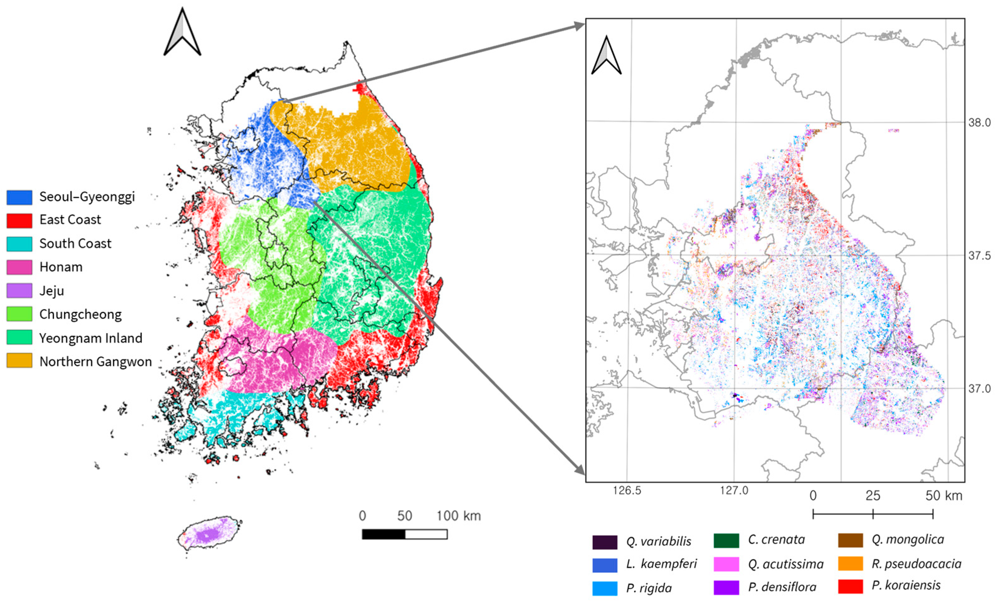
Before model development, the forest regions were delineated using the updated 2023 DFTM provided by the Korea Forest Service, to account for regional variations in species distribution resulting from climatic and environmental heterogeneity [28]. From the DFTM, 43 forest tree species classified as forest stands were selected as analytical targets. The nationwide spatial distribution of each species was estimated using kernel density estimation. The results were converted into density maps with a 100 × 100 m grid resolution. To restrict the study area, the derived density maps were clipped to the forest boundaries defined in the DFTM. We integrated kernel density maps of all species groups and performed cluster analyses to identify regions with similar forest tree species compositions. All the density maps were standardized before clustering, and an unsupervised k-means algorithm was then applied. The optimal number of clusters was evaluated based on the within-cluster sum of squares (WSS) for different cluster numbers [29,30]. We selected eight clusters at the elbow point where the reduction in WSS began to diminish.

2.1.2. Seoul–Gyeonggi Region

The Seoul–Gyeonggi region (37° N, 127° E) was selected as the pilot study region to develop a training-data optimization framework. The study area encompasses approximately 258,381 ha of temperate forests (Figure 2). This region has diverse forest types and topographic conditions, with elevations ranging from 3.2 to 906.4 m. Based on the DFTM, nine dominant forest tree species were selected for classification, focusing exclusively on single-species-dominated stands where the target species comprises at least 70% of the canopy cover. The selected species included four coniferous species (Pinus rigida, Pinus densiflora, Pinus koraiensis, and Larix kaempferi) and five deciduous species (Quercus acutissima, Quercus variabilis, Quercus mongolica, Robinia pseudoacacia, and Castanea crenata). Collectively, these nine species occupy 100,782.1 ha, representing approximately 39% of the total forest area in the Seoul–Gyeonggi region. The species distribution within the study area was as follows: P. rigida (23.3%), L. kaempferi (16.9%), P. densiflora (15.6%), P. koraiensis (15.1%), Q. acutissima (8.3%), R. pseudoacacia (6.3%), Q. variabilis (5.3%), Q. mongolica (4.6%), and C. crenata (4.7%).

2.2. Training Data Collection and Preprocessing

2.2.1. Training and Test Set Sampling Strategy

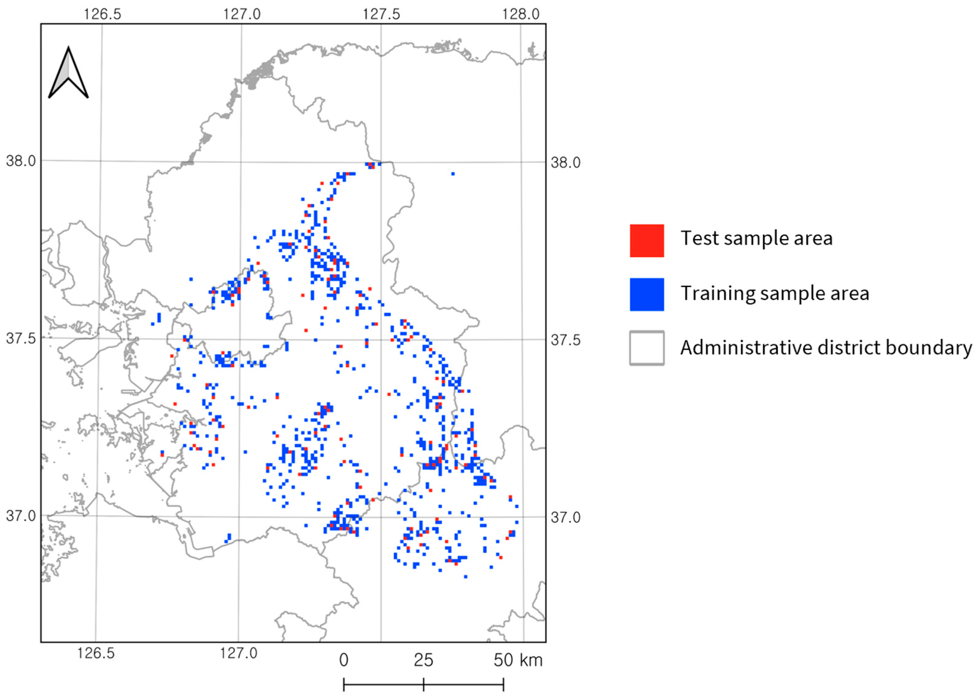
The study area was partitioned using a 1 × 1 km fish-net grid. Valid cells for analysis were selected based on two criteria: target species coverage exceeding 30% of the cell area and the absence of classification errors in the reference data, as determined through visual interpretation of high-resolution satellite imagery. To ensure spatial representativeness and avoid sampling bias toward particular regions, we systematically selected valid cells for the training and test sets. Each grid cell was treated as an independent spatial block to minimize spatial dependence between datasets [31]. The training samples comprised 29.17% of the total area of the nine species in valid cells. Test samples were then collected from the remaining cells, constituting 5.06% of the total nine species area, which enabled the evaluation of the relationship between training sample size and model performance (Figure 3).

2.2.2. Sentinel-2 Imagery

We acquired Sentinel-2 Level-2A atmospherically corrected imagery for 2022–2024 using the Google Earth Engine platform. We selected three periods representing distinct phenological stages. May imagery captures the leaf development stage when deciduous species begin greening, while avoiding March–April periods when high-elevation areas retain snow cover. September imagery represents the full-canopy development stage following the East Asian monsoon. November imagery captures the early leaf-off stage when spectral contrast between deciduous and evergreen species is maximized. Additional temporal acquisitions beyond three selected dates may provide redundant information with minimal accuracy improvements [32]. To ensure cloud-free coverage, we selected scenes with cloud coverage below 60% and applied cloud masking using the QA60 and Scene Classification Layer (SCL) bands. We then calculated the median value across all valid observations to create seamless composite images.
We used eight spectral bands, all of which were resampled to a 10-m spatial resolution. These included the visible blue (B2), green (B3), and red (B4) bands; the Red Edge band (B5); the near-infrared band (B8); and the shortwave infrared bands of water vapor (B9), SWIR1 (B11), and SWIR2 (B12). Bands originally at 20-m resolution (B5, B11, B12) and 60-m resolution (B9) were resampled using bilinear interpolation to maintain spatial consistency across all input features. While resampling may introduce some blurring of spectral signatures, the empirical evidence from Cha et al. (2023) suggests that the additional spectral information from these bands outweighs the potential loss from resampling [25].
Seven vegetation indices were computed from the collected satellite imagery for each seasonal composite data: normalized difference vegetation index (NDVI), green NDVI (GNDVI), ratio vegetation index (RVI), normalized difference Red Edge (NDRE), chlorophyll index Red Edge (CIre), modified chlorophyll absorption ratio index (MCARI), and soil-adjusted vegetation index (SAVI) [20,24,33,34,35].
N D V I = N I R R e d N I R + R e d
G N D V I = N I R G r e e n N I R + G r e e n
R V I = N I R R e d
N D R E = N I R R e d   E d g e N I R + R e d   E d g e
C I r e = N I R R e d   E d g e 1
M C A R I = R e d   E d g e R e d 0.2 R e d   E d g e G r e e n R e d   E d g e R e d  
S A V I = N I R R e d N I R + R E D + 0.5 1 + 0.5
Texture analysis was performed using the gray-level co-occurrence matrix (GLCM) method with the NIR band, which typically shows the highest contrast in forest vegetation. To determine the optimal window size, we conducted a comparative analysis using 3 × 3, 5 × 5, and 7 × 7 pixel windows, with GLCM features used as the sole input to the U-Net model. The results showed no significant differences in classification accuracy across the three window sizes (Table A1). Given these comparable results and considering that the 3 × 3 window size is widely adopted in vegetation classification studies for its effectiveness and computational efficiency [36,37], we selected the 3 × 3 window for our analysis. This small kernel preserves essential local textural information in our fragmented and topographically complex forest areas while minimizing over-smoothing. Therefore, the GLCM analysis in the final workflow used a 3 × 3 pixel window with a displacement of 1 pixel, calculated for four directions (0°, 45°, 90°, and 135°) and averaged to achieve rotation invariance. The NIR values were quantized to 16 gray levels to balance computational efficiency with texture detail preservation. Seven texture features were extracted from each GLCM: contrast, dissimilarity, homogeneity, energy, correlation, angular second moment, and entropy [38,39,40]. These features capture different aspects of the spatial patterns characteristic of the canopy structures of various forest species.
The feature stack comprised 66 channels, consisting of 22 features: 8 spectral bands, 7 vegetation indices, and 7 texture features, for each of the 3 seasonal periods. The final feature stacks were processed as 64 × 64 pixel patches extracted from each 1 × 1 km image. Four overlapping patches were extracted from the corners of each 100 × 100-pixel grid cell to ensure spatial coverage while maximizing data utilization. After excluding the separately sampled test sets, geometric augmentation was applied to capture the rotation-invariant nature of the forest patterns, including vertical flips, horizontal flips, and rotations (90° and 270°). Including the original orientation, this increased the training data by a factor of five. The augmented training dataset was divided into 80% training and 20% validation.

2.2.3. Label Data

In DFTM, areas are designated by species names when a single species constitutes 70% or more of the canopy cover. Meanwhile, mixed species stands or regions dominated by minor species are classified into broader categories, such as other broadleaf forests or other coniferous forests. Given our objective for species-level classification, we excluded these generalized categories from the analysis. To improve label purity, we further refined the DFTM by manually correcting or excluding polygons containing other species based on multiple high-resolution satellite imagery (Kakao Map, vWorld, and Google Satellite layers available in QGIS 3.40.5-1). This manual screening was particularly important in the Seoul–Gyeonggi region, where numerous restricted or unverified areas (e.g., military zones) are present. The refined map was then converted into a 10-m raster format to match the spatial resolution of the Sentinel-2 imagery, resulting in a label dataset comprising nine forest tree species and background pixels.
To evaluate the reliability of the final label dataset, we conducted a stratified random accuracy assessment using 68 validation pixels per species class, which represents a 90% confidence level with a 10% margin of error. The validation indicated species-specific label noise ranging from 1.47% to 8.82% (Table A2), demonstrating the overall reliability of the training data. Label noise was mainly observed in areas with complex species intermixing. Among all species, R. pseudoacacia exhibited the relatively high structural overlap with neighboring species.

2.3. Deep-Learning Model Implementation

2.3.1. U-Net Model Architecture

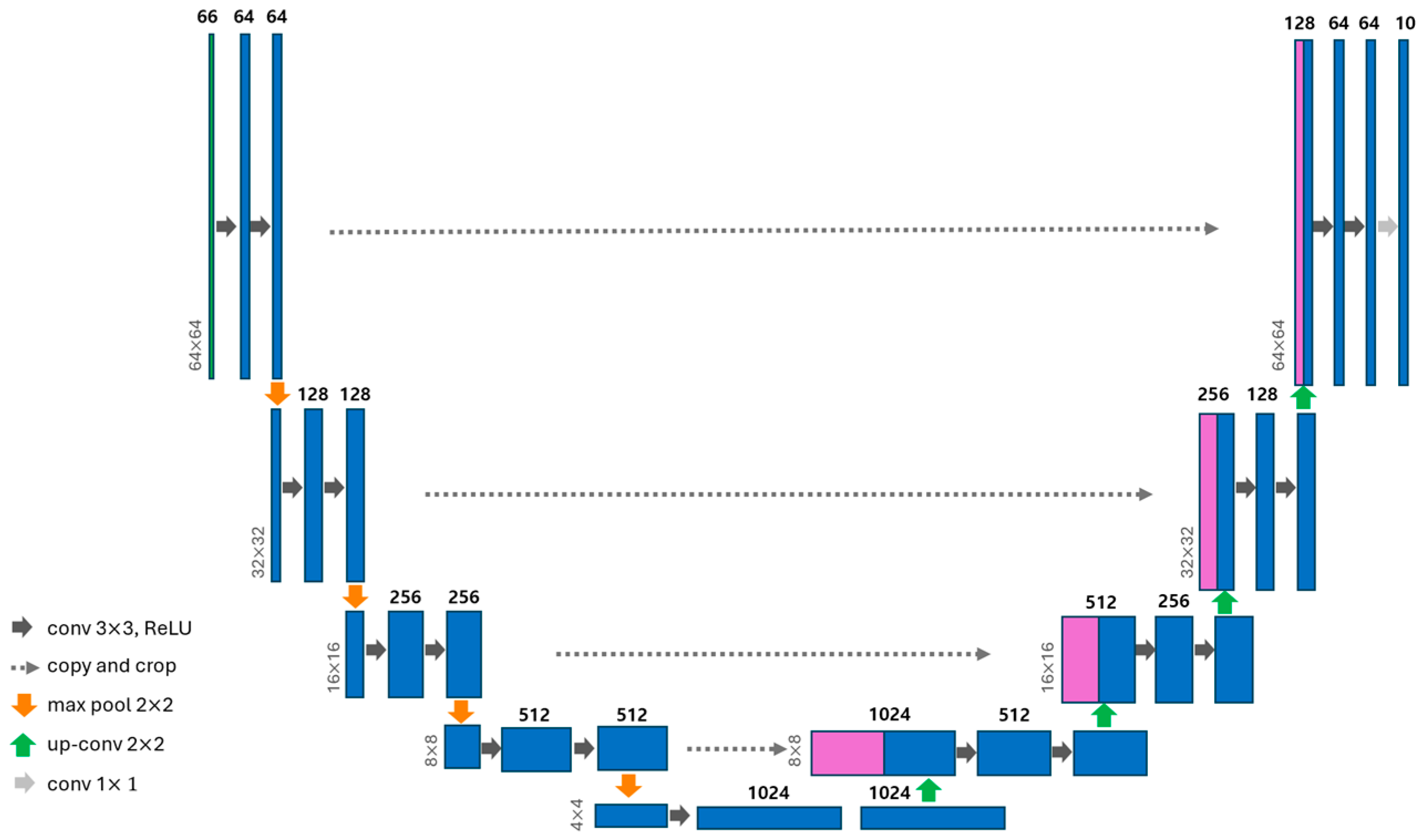
We implemented a U-Net model comprising a contracting encoder path and an expansive decoder path connected by skip connections (Figure 4). The encoder consisted of four downsampling stages, with channel dimensions ranging from 64 to 128, 256, and 512. Each stage consisted of two 3 × 3 convolutional blocks with batch normalization and ReLU activation, followed by 2 × 2 max pooling for spatial down-sampling. The bridge layer at the bottom was connected to the encoder and decoder by 1024 channels. The decoder path mirrored the encoder through four up-sampling stages using 2 × 2 transposed convolutions. Skip connections concatenate encoder features with up-sampled decoder features to preserve the fine-grained spatial information lost during down-sampling. The channel dimensions symmetrically decreased from 512 to 64. A final 1 × 1 convolution layer produced 10-class predictions, that is, nine forest tree species plus the background. The U-Net model was configured to output ten classes (0–9) to maintain consistent tensor dimensions across all patches, where class 0 represents background and classes 1–9 correspond to forest types.
During data preprocessing, all background and NoData pixels (label = 0) were assigned a value of −9999 and excluded from percentile-based normalization and global statistics. Before training, these background pixels were converted to −100 in the label arrays, which was set as the ignore_index parameter in the cross-entropy loss. Consequently, although the network outputs ten class probabilities, the loss and metric computations entirely ignore pixels labeled −100 (i.e., background), and optimization is driven only by valid forest classes (1–9).
Training utilizes a weighted cross-entropy loss function with class weights that are inversely proportional to species frequencies to mitigate class imbalance. We optimized the model using the Adam optimizer with an initial learning rate of 0.001. We implemented a learning rate scheduler that reduced the learning rate by 50% when the validation accuracy plateaued for five epochs, with a minimum learning rate threshold of 1 × 10⁻⁶. The model was trained for a maximum of 100 epochs, with early stopping (patience = 10) to prevent overfitting. The training was conducted with a batch size of eight.

2.3.2. Incremental Training Experiment Design

To evaluate the relationship between training sample size and model performance, we conducted incremental training experiments, progressively increasing the amount of data. The total number of cells available for training, representing 29.17% of the total study area with the target species coverage, was 728. For computational simplicity, we used an image-count-based sampling approach. The experiment began with minimal training samples (1, 5, 10, 20, 40, 60, 80, …, 200) to assess performance in limited data scenarios. To ensure robust results and account for variability in random sampling, we performed three independent runs with different random seeds for configurations up to 200 images. This resulted in a total of 50 training sample size configurations (1, 5, 10, 20, 40, 60, 80, 100, 120, 140, 160, 180, and 200 images × 3 seeds, plus additional configurations from 250 to 728 images in increments of 50).
We randomly selected these specific numbers of cells from a full pool of 728 training cells. Following each training iteration, we calculated the percentage distribution area for each of the nine species used for training relative to the total distribution area in the Seoul–Gyeonggi region, defined as the training sample size. Since each random ordering resulted in different combinations of cells with varying species coverage, the actual training area percentages differed across seeds. Rather than averaging these results, we treated each run as an independent data point, creating multiple area-performance observations. This approach provided a richer dataset for analyzing the relationship between training area percentage and model performance, with particularly dense sampling in the critical low-data regime (1–200 images).

2.3.3. Model Performance Evaluation

The model’s performance was evaluated using the test set and the following metrics: overall accuracy (OA), which measures the proportion of correctly classified pixels across all classes, as follows:
O A = i = 1 c T P i i = 1 c T P i + F P i + F N i + T N i
where C is the number of classes, TP is the true positive, FP is the false positive, FN is the false negative, and TN is the true negative of each class i.
The F1-score for each species was calculated as the harmonic mean of the precision and recall.
F 1 i = = 2 × P r e c i s i o n i × R e c a l l i P r e c i s i o n i + R e c a l l i
where P r e c i s i o n i = T P i T P i + F P i   and R e c a l l i = T P i T P i + F N i for each class i.
The Macro F1-score was then computed by averaging the species-specific F1-scores without weighting:
Macro   F 1   score =   1 C i = 1 c F 1 i
Confusion matrix analysis was performed on the best-performing model (with the highest overall accuracy, OA) to identify species-specific classification patterns and interspecific confusion.

2.3.4. Optimal Training Sample Size Analysis

To analyze the relationship between training sample size and model performance, we applied locally estimated scatterplot smoothing (LOESS) regression with a span parameter of 0.6 to the results from 50 different training sample sizes. LOESS was selected because of its ability to capture nonlinear relationships without assuming a specific functional form. This provides a smooth curve that reduces the influence of random sampling variations at individual training sizes.
From the fitted LOESS curve, we defined the optimal training sample sizes as the points achieving 90% and 95% of the maximum performance, representing efficient resource utilization with sufficient accuracy. These optimal points were assessed using both the Macro F1-score and overall accuracy (OA). Species-specific F1-scores were analyzed to examine the variations in optimal training sample sizes across different forest tree species. To examine how the fitted trend was different on the choice of functional form, several additional curve-fitting models (logarithmic, power-law, Michaelis–Menten, and exponential saturation) were also tested, as detailed in the Supplementary Materials.

3. Results

3.1. Optimal Training Sample Size and Maximum Accuracy

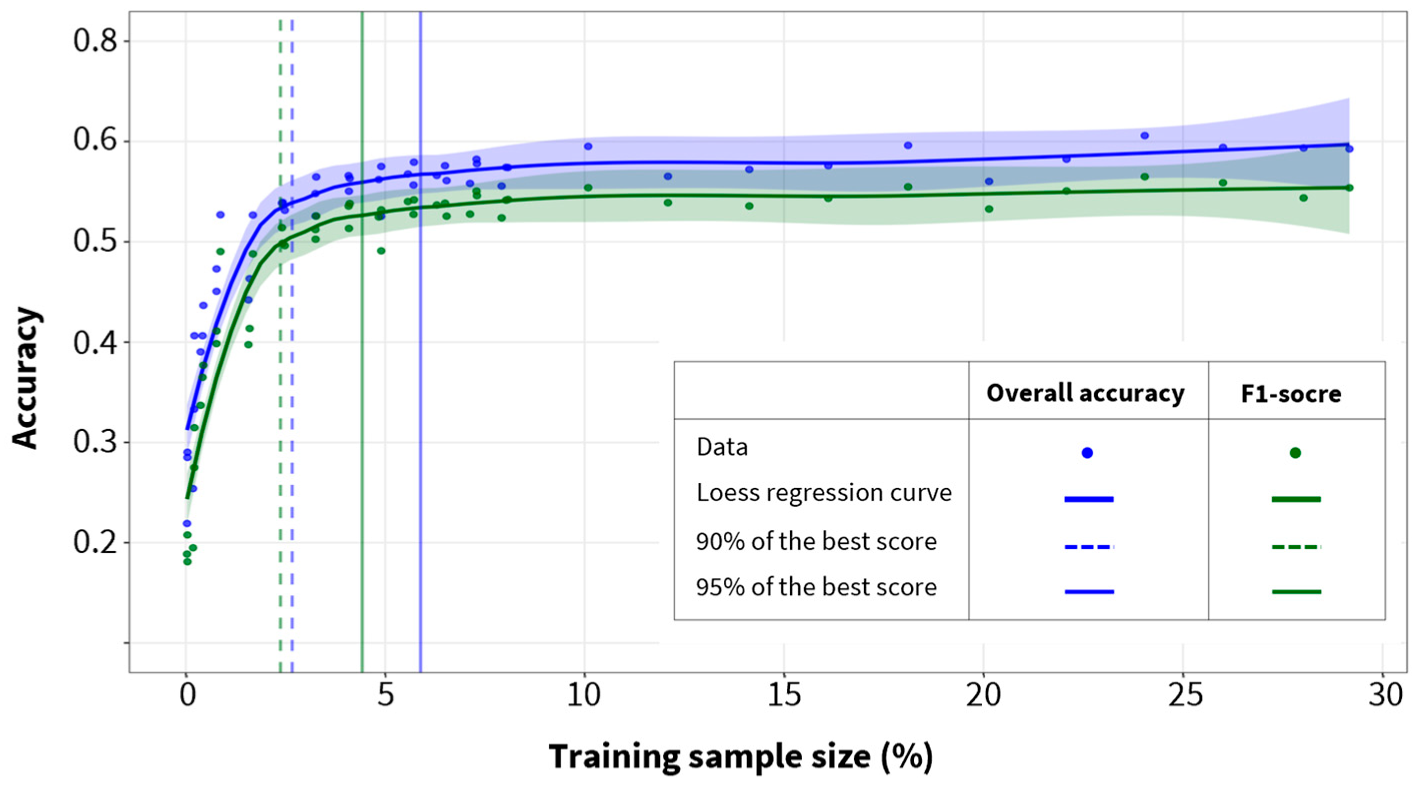
Three distinct stages characterize the relationship between the training data size and model performance: rapid improvement, gradual saturation, and plateau (Table A3, Table A4 and Table A5, Figure 5). Both the OA and macro F1-score metrics demonstrated diminishing returns as the training sample size increased. The maximum observed accuracy reached 61% (F1-score: 0.56) with a training sample size of 24.04% (600 images).
In the early stages, the model demonstrated rapid accuracy improvements with minimal training data. Based on random seed = 42 (Table A3), starting with a baseline OA of 22% and an F1-score of 0.19 (0.03% training sample size, one sample image), the performance improved rapidly. It achieved 45% accuracy (F1-score: 0.41) with a training sample size of 0.77% (20 images). The performance continued to increase substantially, reaching 55% accuracy (F1-score: 0.51) with a 3.25% training sample size (80 images). This stage demonstrates the highest efficiency in terms of performance gain per additional training sample.
In the saturation stage, the performance improvements began to decelerate despite the increase in training sample size. For overall accuracy, the model achieved 90% and 95% of its maximum performance at 2.67% (95% CI: 1.79%–3.40%) and 5.89% (95% CI: 2.96%–11.76%) of the training sample data, respectively. The macro F1-score reached similar saturation levels at slightly lower training sample sizes: 2.37% (95% CI: 1.79%–3.25%) for 90% of its maximum performance and 4.42% (95% CI: 2.52%–7.06%) for 95% of its maximum performance.
Beyond the optimal points, a performance plateau was observed where additional training data yielded negligible performance improvements. For example, increasing the training sample size by nearly fourfold from 5.45% to 24.04% only improved the OA by 3.65%. Throughout this plateau stage, performance fluctuated within narrow ranges: 56–61% for OA and 0.53–0.56 for the F1-score. To assess performance stability, we examined variability across the three stages (Appendix A Table A6). While variability was high for very small training sizes, dispersion became minimal in the plateau regime (SD ≤ 0.015), confirming that the learning curve had converged and that the performance ceiling is stable. The detailed numerical values can be found in Appendix A Table A3, Table A4 and Table A5, and the results fitted with alternative model types are presented in the Supplementary Materials.

3.2. Species-Specific Classification Accuracy and Confusion Patterns

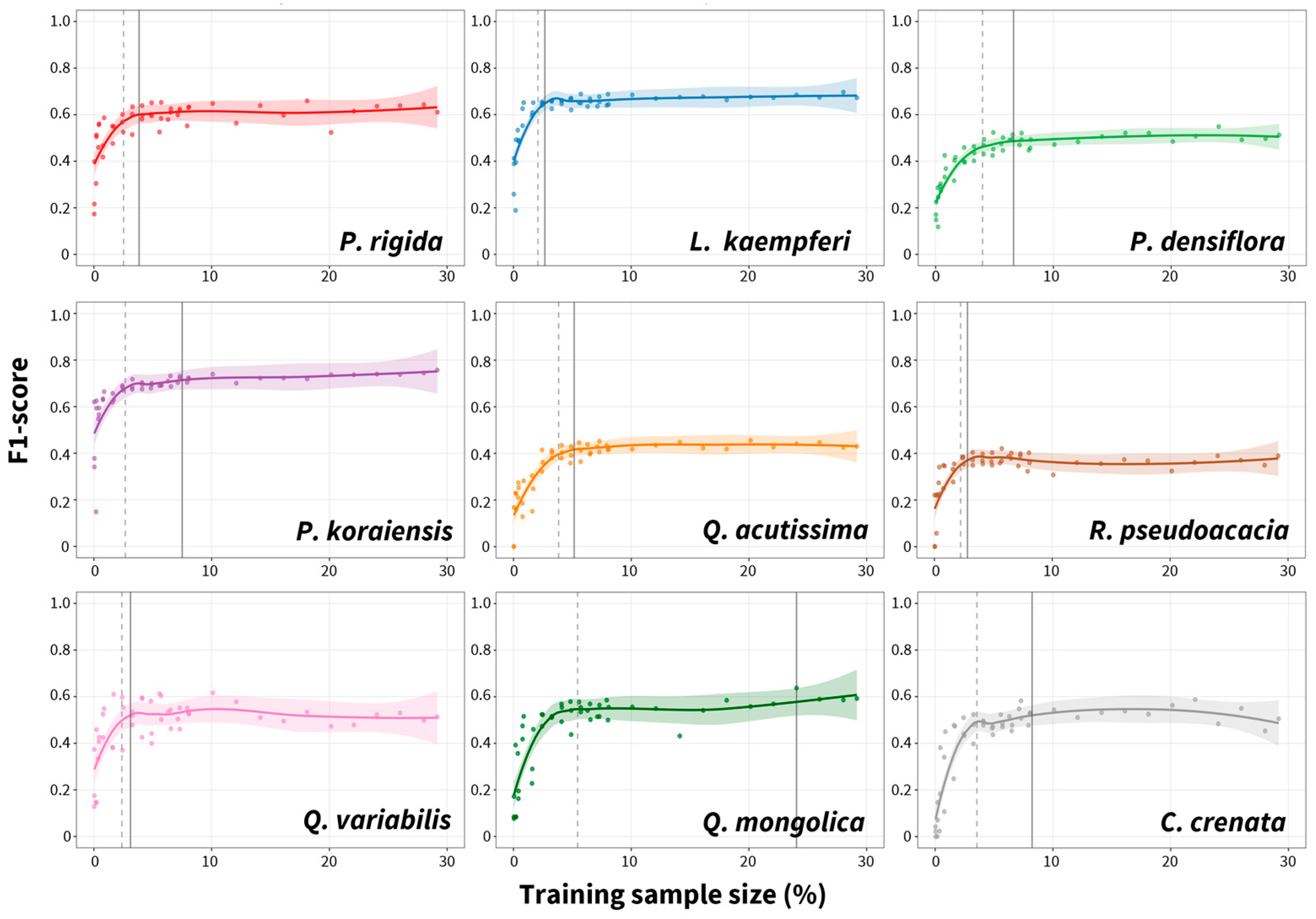
The species-specific performance curves showed generally consistent patterns across most species (Figure 6). The training sample size required to achieve 90% of the maximum performance ranged from 2.08% to 5.45% (mean: 3.19%; median: 2.67%). The 95% threshold exhibited greater variability, ranging from 2.67% to 24.04% (mean: 7.77%; median: 5.16%). Q. mongolica was a clear outlier, requiring 24.04% of the training area to reach 95% of the maximum performance. Excluding this outlier, the remaining eight species reached 95% of the maximum performance between 2.67% and 8.23% (mean: 5.37%). For most species, the difference between the 90% and 95% thresholds ranged from 0.58% to 4.83%.
The maximum F1 scores also varied notably among species. Based on their peak performance, species were categorized into three groups. High-performing species (F1 > 0.7) included P. koraiensis (0.75) and L. kaempferi (0.68), both achieving 90% performance with less than 3% of the training area. Medium-performing species (0.5 ≤ F1 ≤ 0.7) included P. rigida (0.63), Q. mongolica (0.61), Q. variabilis (0.55), C. crenata (0.55), and P. densiflora (0.51). Low-performing species (F1 < 0.5) were Q. acutissima (0.44) and R. pseudoacacia (0.39).
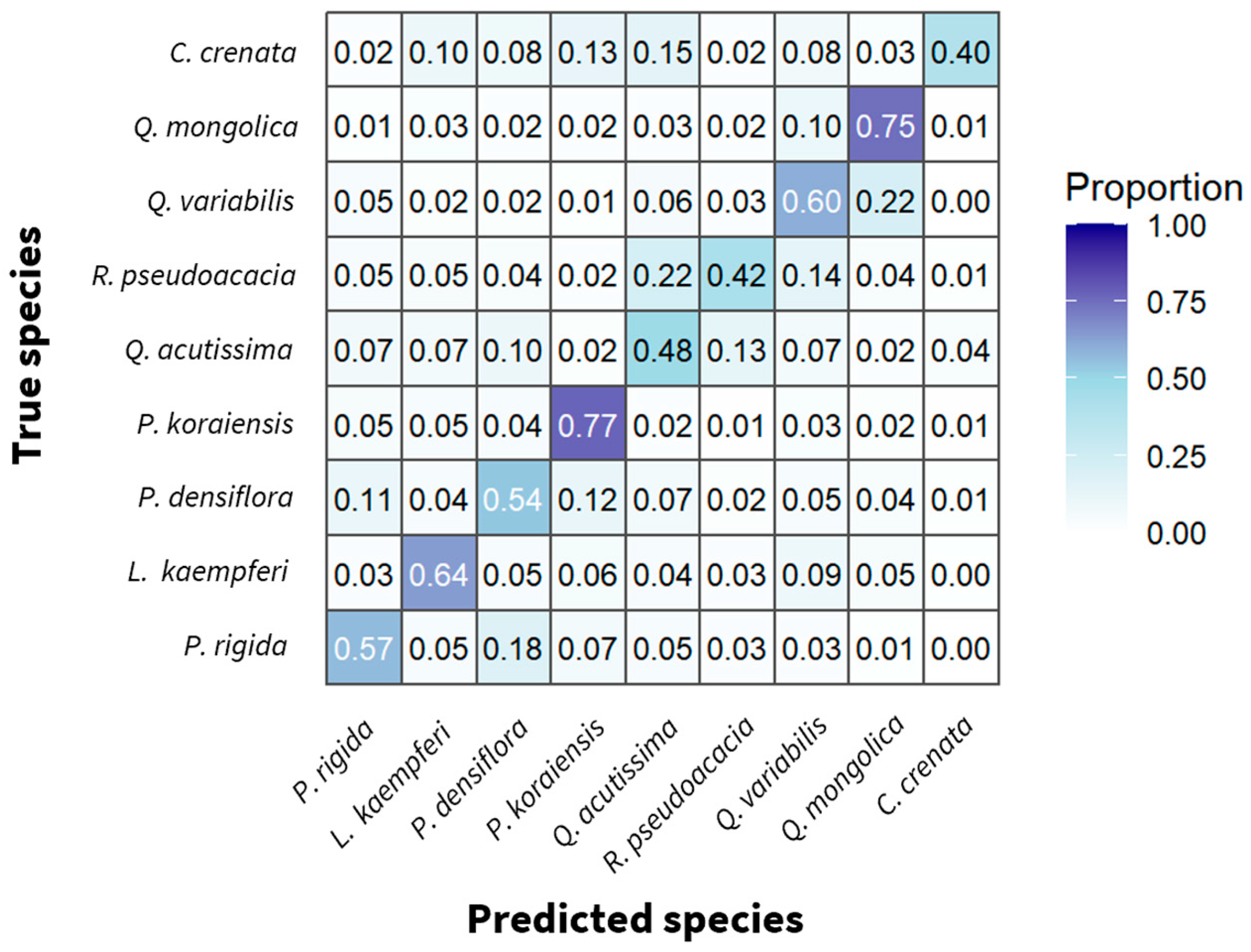
To identify misclassification patterns for low-performing species, we examined the confusion matrix of the best-performing model (600 training images, 61% OA; Figure 7). Major confusion patterns were observed between particular species pairs. The most substantial misclassification occurred between P. rigida and P. densiflora, with 18.3% of P. rigida reference pixels being incorrectly classified. P. densiflora was often confused with P. koraiensis (11.7%) and P. rigida (11.0%). This indicates high spectral similarity among these three coniferous species. Q. variabilis and Q. mongolica demonstrated bidirectional confusion, with 21.8% of Q. variabilis being misclassified as Q. mongolica, and 10.4% of Q. mongolica being misclassified as Q. variabilis. Q. acutissima and R. pseudoacacia exhibited mutual confusion patterns, with 13.2% of Q. acutissima misclassified as R. pseudoacacia and 22.0% of R. pseudoacacia misclassified as Q. acutissima. L. kaempferi showed a relatively balanced classification with 63.9% accuracy, although confusion occurred with Q. variabilis (misclassification of 8.8%). C. crenata presented the most dispersed misclassification pattern with substantial confusion across multiple species, where the highest confusion rates were observed in Q. acutissima (15.0%), P. koraiensis (12.7%), and L. kaempferi (9.9%).
Table 1 summarizes the per-species precision, recall, and F1-scores of the model trained with 24.04% of the available samples (random seed = 42). Among the nine target species, P. koraiensis achieved the highest F1-score (0.74) with both high precision (0.71) and recall (0.77). L. kaempferi and P. rigida also showed relatively balanced and moderate performance (F1 = 0.69 and 0.64, respectively). In contrast, Q. acutissima and R. pseudoacacia yielded the lowest F1-scores (0.44 and 0.39), mainly due to mutual confusion and low recall, consistent with the confusion patterns described in Figure 7. C. crenata exhibited low recall (0.39) and moderate precision (0.62). The remaining deciduous oaks (Q. variabilis and Q. mongolica) achieved intermediate F1-scores (0.52–0.64).

4. Discussion

4.1. Optimal Training Sample Size for Forest Tree Species Classification

Our results show that 90% of maximum accuracy is achieved with a training sample size of 2.37%–2.67%, with an increase of approximately 3% needed to reach 95% of the maximum accuracy at 4.42%–5.89%. Accordingly, we recommend a threshold of 4.42%–5.89% as the optimal training sample size for operational forest species mapping. The identified optimal point, approximately 5.5% of the total area for the 9 species, represents a critical threshold for regional forest species mapping, which can be translated to 554,301 pixels, excluding the background. This substantially exceeds the training sample sizes used in previous land cover classification studies. Zhu et al. (2016) achieved accuracy saturation at approximately 20,000 pixels when mapping land cover across the continental United States using Landsat imagery [11]. Ramezan et al. (2021) tested training sets ranging from 40 to 10,000 pixels across a 260,975 ha study area, finding minimal accuracy improvement for Random Forest but continued gains for support vector machine (SVM) at 10,000 pixels [12].
While previous studies have focused on land cover classification, the requirement for substantially higher pixel counts in our study may be attributed to the more complex nature of species-level differentiation. Species-level classification among spectrally similar forest tree species requires capturing more subtle spectral and textural variations than broad land cover categories, necessitating larger training datasets to represent both intra-species variability and inter-species differences adequately. Furthermore, the difference in model architecture contributes to increased data requirements. Previous studies have employed traditional machine learning models, such as RF and SVM, that classify individual pixels or small patches independently. In contrast, our U-Net model processes entire image tiles through its fully convolutional architecture, which requires a spatial context to learn hierarchical features across multiple scales.
Selecting the 95% threshold represents an optimal balance between accuracy and efficiency, with performance plateauing beyond this point. This plateau indicates that additional training data provide redundant information rather than new spectral signatures. These findings have critical operational implications for training data collection that can be optimized rather than maximized. The 5.5% training sample size provided a transferable benchmark for developing forest tree species classification models for other regions. Areas with small coverage would require proportionally fewer training samples, while extensive regions require correspondingly more training samples to achieve comparable classification accuracy. However, since this study focuses on a site-specific model developed for the Seoul–Gyeonggi region, the derived results reflect regional characteristics. Therefore, these relationships should be further validated to assess their transferability to other ecological regions.

4.2. Species Classification Performance and Limiting Factors

In this study, we achieved a maximum OA of 61% and an F1-score of 0.56, which aligns with previous national-scale forest classification efforts. Lee et al. (2023) reported a similar F1-score of 0.53 for nine species across South Korea using Sentinel-2 imagery [13]. In contrast, studies with fewer species have achieved considerably higher accuracies: 80–90% for five species across 1500 ha in Sweden [32], 87% for four species in southern Sweden [42], and 90% for four species in the Qilian Mountains, China [24]. This pattern suggests that classification complexity can increase with the number of species due to the compounding of spectral overlaps and within-species variability.
Confusion matrix analysis showed that spectral similarity among congeneric species was the primary factor limiting classification accuracy. The Pinus species complex (P. rigida, P. densiflora, P. koraiensis) exhibited the highest confusion rates, with substantial misclassification between P. rigida and P. densiflora (18.3%). The bidirectional confusion between Quercus species reached 21.8%. This high misclassification rate can be attributed to the inherent spectral similarities between species within the same genus and their comparable phenological patterns [13,43]. However, hyperspectral imagery substantially improves the species-level classification accuracy [5]. While multispectral imagery has inherent limitations in discriminating closely related species within the same genus, hyperspectral sensors can detect subtle spectral differences between species because of their numerous spectral bands [5,44,45,46]. Moreover, the classification accuracy can be further enhanced through integration with complementary data sources such as LiDAR and SAR [5,44,45,47].
Our three-date temporal composite approach, spanning May, September, and November, was designed to capture key phenological transitions while balancing classification performance with computational efficiency. However, the median compositing approach across 2022–2024, while necessary to ensure cloud-free coverage, may have further dampened these phenological signals. Additionally, alternative temporal combinations could potentially yield comparable results depending on local phenological timing and species composition. Future studies could explore different month combinations and denser temporal sampling to further improve species discrimination.
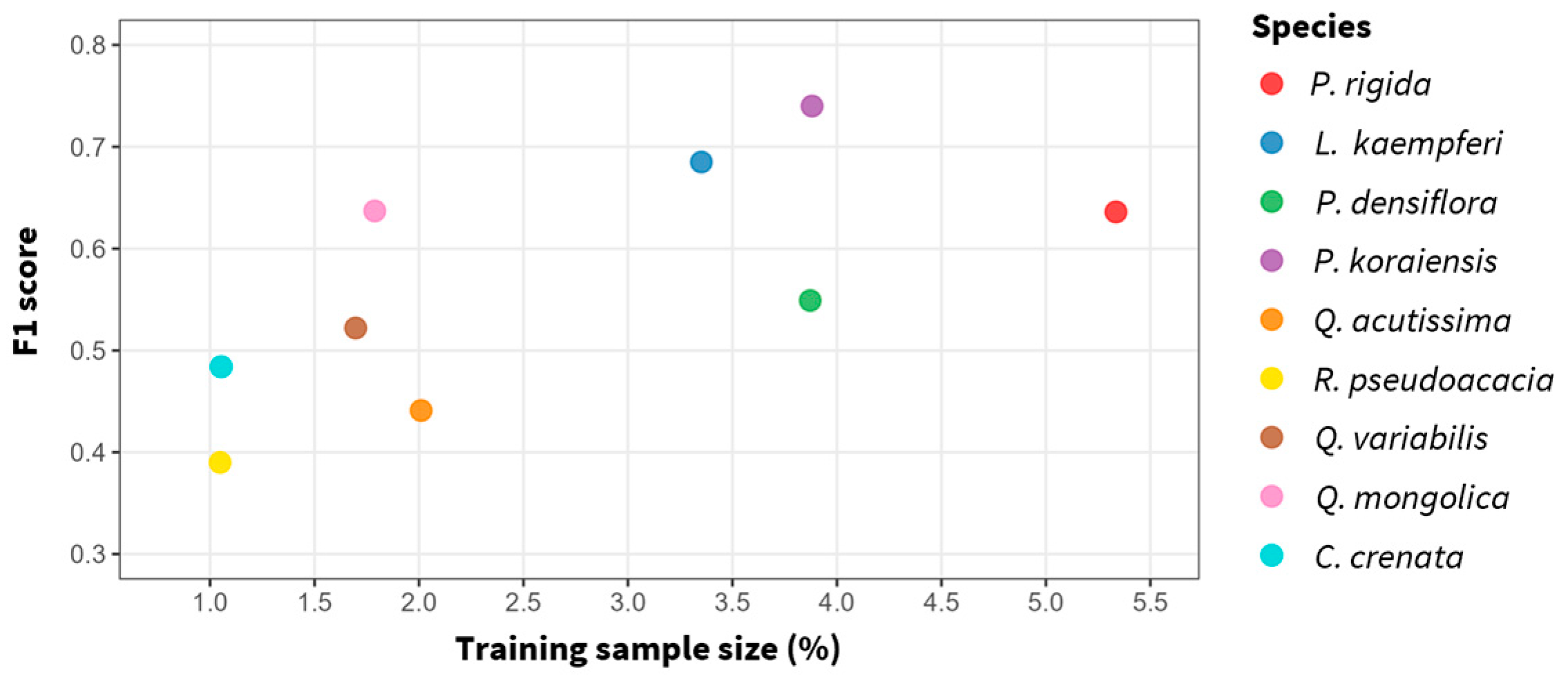
Species prevalence is another critical factor affecting classification accuracy. In Hemmerling et al. (2021), dominant species with >0.5% area coverage achieved accuracies of 66.8%–98.9%, whereas for minor species, accuracy fell to 14.8%–68.4% [46]. Our findings mirror this pattern, with C. crenata and R. pseudoacacia representing the smallest training areas in our dataset and achieving low maximum F1-scores: C. crenata (0.55) and R. pseudoacacia (0.40) (Figure 8). This suggests that a sufficient training sample size is a prerequisite for reliable species classification and that the imbalanced distribution of species in natural forests poses a fundamental challenge for remote sensing applications. These findings highlight the need for data augmentation techniques, such as geometric transformations, as implemented in our study, to balance the training datasets. However, more systematic sampling approaches, such as stratified equal random sampling, may further improve minority species classification [48].
Beyond methodological considerations, fundamental data might establish the observed performance ceiling. When the DFTM is created, polygons are labeled with the dominant species name when a single species comprises over 70% of the area, and field surveys are conducted to verify this 70% threshold criterion. However, to obtain clean training data, we modified the label data through visual interpretation to ensure each polygon unambiguously represents a single species class. Nevertheless, since our verification relied on satellite imagery interpretation, there remain areas where tree crowns overlap due to canopy structure, and locations where different species are intermixed. In addition, at the Sentinel-2 10-m resolution, individual pixels integrate spectral signatures from multiple tree crowns, further obscuring species-specific features. Variations in canopy density within the 10-m pixels result in different contributions from exposed soil and understory vegetation signals, which may further limit species differentiation [49].
While training samples were evenly distributed across the study region to capture diverse terrain and forest conditions, environmental factors such as stand age, topography, and forest origin (natural vs. planted) were not explicitly modeled in the analysis. The systematic sampling strategy may have indirectly incorporated some of this variability, but the unquantified effects of these factors on canopy structure, illumination conditions, and spectral purity represent an additional source of classification uncertainty beyond the inherent data limitations.
Topographic variation, in particular, can affect canopy reflectance and texture by altering illumination geometry and shadowing [50,51]. Although topographic variables were not explicitly included, the multi-temporal Sentinel-2 L2A imagery (May, September, and November) partially captures illumination variability caused by terrain effects. However, previous studies have shown that adding DEM-derived variables or applying topographic correction can improve forest species classification accuracy [52,53]. Future work should therefore consider integrating terrain-related predictors to enhance model robustness in complex terrain.
These inherent constraints, that is, spectral resolution limitations, temporal sampling density, mixed pixel effects arising from spatial resolution, and sampling strategy, suggest that the 61% accuracy achieved in this study represents a practical upper limit for regional-scale forest type mapping using medium-resolution satellite imagery, rather than a limitation of training data quantity or model capacity.

5. Conclusions

This study provides empirical evidence to guide the optimization of training data collection for operational mapping of forest species using the U-Net model with Sentinel-2 imagery. We evaluated 50 training sample sizes ranging from 0.03% to 29.17% of the species’ total distribution area. The optimal sample sizes for training were 2.37%–2.67% for 90% maximum accuracy and 4.42%–5.89% for 95% maximum accuracy, beyond which additional training data yielded minimal improvements in accuracy. Given this increment in the training sample size required to achieve 90%–95% maximum accuracy, a 95% threshold training sample size of approximately 5.5% is recommended for efficient model development. The maximum achieved accuracy was 61%, which represents a practical ceiling for regional-scale species classification using 10 m-resolution satellite imagery. These limitations are due to spectral, temporal, and spatial resolutions. Complementary approaches are required to address these constraints, such as hyperspectral sensor fusion for enhanced spectral discrimination, denser temporal acquisition for phenological characterization, and the use of data with finer spatial resolution to reduce mixed-pixel effects. Despite these accuracy limitations, the identified 5.5% threshold provided valuable practical guidance for operational forest monitoring. This information will help to prevent under-sampling and redundant data collection, enabling forest monitoring programs to prioritize methodological improvements over extensive training data collection beyond the optimal training sample size. Although our findings were derived from South Korean forests and require validation across diverse forest ecosystems to determine broader applicability, they represent an essential contribution toward optimizing deep-learning applications in forest tree species monitoring.

Supplementary Materials

The following supporting information can be downloaded at: https://www.mdpi.com/article/10.3390/f16111718/s1, Figure S1: Relationship between training sample size and model performance for four curve types (LOESS, logarithmic, power-law, Michaelis–Menten, and exponential saturation); Table S1: Model-fitting performance and estimated training sample size thresholds for four curve types.

Author Contributions

Conceptualization, H.L.; Methodology, H.L. and C.L.; Validation, H.L. and S.-E.C.; Formal analysis, H.L. and C.L.; Investigation, H.L.; Data curation, H.L.; Writing—original draft preparation, H.L. and C.L.; Writing—review and editing, S.-E.C. and H.W.; Visualization, H.L.; Supervision, S.-E.C.; Project administration, S.-E.C.; Funding acquisition, H.W. All authors have read and agreed to the published version of the manuscript.

Funding

This research was conducted with support from the National Institute of Forest Science research on forest-specific information based on the integration of CAS500-4 satellite data (FM0103-2021-04-2025).

Data Availability Statement

Data is contained within the article. The original codes used for Sentinel-2 image processing, U-Net model implementation, and dataset preparation are openly available at https://github.com/heejae0110/tree_species_classification_u-net.

Conflicts of Interest

The authors declare that they have no conflicts of interest. The funders had no role in the design of the study, in the collection, analysis, or interpretation of data, in the writing of the manuscript, or in the decision to publish the results.

Abbreviations

The following abbreviations are used in this manuscript:
CNNConvolutional neural network
DFTMDigital forest type map
LOESSLocally estimated scatterplot smoothing
GLCMGray-level co-occurrence matrix
WSSWithin-cluster sum of squares
NDVINormalized difference vegetation index
GNDVIGreen normalized difference vegetation index
RVIRatio vegetation index
NDRENormalized difference red edge
CIreChlorophyll index red edge
MCARIModified chlorophyll absorption ratio index
SAVISoil-adjusted vegetation index
OAOverall accuracy
TPTrue positive
FPFalse positive
FNFalse negative
TNTrue negative
NIRNear-infrared
SWIRShortwave infrared
SCLScene classification layer
QAQuality assessment

Appendix A

Table A1. Performance comparison of different GLCM window sizes (3 × 3, 5 × 5, 7 × 7) for U-Net tree species classification using 7 GLCM features only: 300 images randomly selected, divided into training, validation, and test sets with 7:2:3 ratio, trained for 50 epochs with three random seeds.
Window SizeTest Accuracy (Mean ± Std)
3 × 30.1827 ± 0.0264
5 × 50.1799 ± 0.0277
7 × 70.1848 ± 0.0245
Table A2. Species-specific label noise percentages derived from the stratified random accuracy assessment.
SpeciesLabel Noise (%)
Pinus rigida2.94
Larix kaempferi5.88
Pinus densiflora4.41
Pinus koraiensis1.47
Quercus acutissima2.94
Robinia pseudoacacia8.82
Quercus variabilis4.41
Quercus mongolica2.94
Castanea crenata4.41
Table A3. Model training results by number of images and training sample size of random seed = 42.
Number of ImagesTraining Sample Size (%)OA (%)Macro F1-Score
10.030.220.19
50.210.330.27
100.420.410.36
200.770.450.41
401.570.440.40
602.430.540.50
803.250.550.51
1004.090.550.51
1204.900.580.53
1405.720.580.54
1606.540.560.53
1807.290.580.55
2008.030.570.54
25010.090.600.55
30012.090.570.54
35014.130.570.54
40016.110.580.54
45018.110.600.55
50020.140.560.53
55022.080.580.55
60024.040.610.56
65026.000.590.56
70028.020.590.54
72829.170.590.55
Table A4. Model training results by number of images and training sample size of random seed = 73.
Number of ImagesTraining Sample Size (%)OA (%)Macro F1-Score
10.040.290.21
50.180.250.19
100.370.390.34
200.770.470.40
401.600.460.41
602.410.540.51
803.270.560.53
1004.110.560.54
1204.900.530.49
1405.710.560.53
1606.500.580.54
1807.300.580.55
2008.080.570.54
Table A5. Model training results by number of images and training sample size of random seed = 93.
Number of ImagesTraining Sample Size (%)OA (%)Macro F1-Score
10.040.290.18
50.220.410.31
100.440.440.38
200.870.530.49
401.680.530.49
602.480.530.50
803.250.530.50
1004.080.570.54
1204.840.560.52
1405.570.570.54
1606.290.570.54
1807.130.560.53
2007.920.560.52
Table A6. Variability of model performance across training-size regimes based on three random seeds.
MetricStageNumber of ImagesTraining Sample Size (%)MeanSDMinMax
Overall
Accuracy
Early1–800.03–3.270.440.1060.220.56
Saturation100–1404.08–5.720.560.0160.530.58
Plateau160–7286.29–29.170.580.0150.560.61
Macro
F1-score
Early1–800.03–3.270.390.1200.180.53
Saturation100–1404.08–5.720.530.0170.490.54
Plateau160–7286.29–29.170.540.0100.520.56

References

  1. Keenan, R.J. Climate Change Impacts and Adaptation in Forest Management: A Review. Ann. For. Sci. 2015, 72, 145–167. [Google Scholar] [CrossRef]
  2. Barbati, A.; Marchetti, M.; Chirici, G.; Corona, P. European Forest Types and Forest Europe SFM Indicators: Tools for Monitoring Progress on Forest Biodiversity Conservation. For. Ecol. Manag. 2014, 321, 145–157. [Google Scholar] [CrossRef]
  3. Kim, H.-S.; Lee, J.; Lee, S.J.; Son, Y. Methodologies for Improving Forest Land Greenhouse Gas Inventory in South Korea Using National Forest Inventory and Model. J. Clim. Change Res. 2024, 15, 427–445. [Google Scholar] [CrossRef]
  4. Lee, S.T.; Chung, S.H.; Kim, C. Carbon Stocksin Tree Biomass and Soils of Quercus Acutissima, Q. Mongolica, Q. Serrata, and Q. Variabilis Stands. J. Korean Soc. For. Sci. 2022, 111, 365–373. [Google Scholar]
  5. Pu, R. Mapping Tree Species Using Advanced Remote Sensing Technologies: A State-of-the-Art Review and Perspective. J. Remote Sens. 2021, 2021, 9812624. [Google Scholar] [CrossRef]
  6. Moraes, D.; Campagnolo, M.L.; Caetano, M. Training Data in Satellite Image Classification for Land Cover Mapping: A Review. Eur. J. Remote Sens. 2024, 57, 2341414. [Google Scholar] [CrossRef]
  7. Sarker, I.H. Machine Learning: Algorithms, Real-World Applications and Research Directions. SN Comput. Sci. 2021, 2, 160. [Google Scholar] [CrossRef]
  8. Hasmadi, M.; Pakhriazad, H.Z.; Shahrin, M.F. Evaluating Supervised and Unsupervised Techniques for Land Cover Mapping Using Remote Sensing Data. Geografia 2009, 5, 1–10. [Google Scholar]
  9. Ahmad, A.; Quegan, S. Comparative Analysis of Supervised and Unsupervised Classification on Multispectral Data. Appl. Math. Sci. 2013, 7, 3681–3694. [Google Scholar] [CrossRef]
  10. Kumar, M.D.; Bhavani, Y.L.; Sahithi, V.S.; Kumar, K.A.; Cheepulla, H. Analysing the Impact of Training Sample Size in Classification of Satellite Imagery. In Proceedings of the 2024 5th International Conference on Data Intelligence and Cognitive Informatics (ICDICI), Tirunelveli, India, 18–20 November 2024; IEEE: New York, NY, USA, 2024; pp. 879–884. [Google Scholar]
  11. Zhu, Z.; Gallant, A.L.; Woodcock, C.E.; Pengra, B.; Olofsson, P.; Loveland, T.R.; Jin, S.; Dahal, D.; Yang, L.; Auch, R.F. Optimizing Selection of Training and Auxiliary Data for Operational Land Cover Classification for the LCMAP Initiative. ISPRS J. Photogramm. Remote Sens. 2016, 122, 206–221. [Google Scholar] [CrossRef]
  12. Ramezan, C.A.; Warner, T.A.; Maxwell, A.E.; Price, B.S. Effects of Training Set Size on Supervised Machine-Learning Land-Cover Classification of Large-Area High-Resolution Remotely Sensed Data. Remote Sens. 2021, 13, 368. [Google Scholar] [CrossRef]
  13. Lee, J.; Yang, T.; Choi, C. Mapping Nine Dominant Tree Species in the Korean Peninsula Using U-Net and Harmonic Analysis of Sentinel-2 Imagery. Korean J. Remote Sens. 2025, 41, 243–260. [Google Scholar] [CrossRef]
  14. Korznikov, K.A.; Kislov, D.E.; Altman, J.; Doležal, J.; Vozmishcheva, A.S.; Krestov, P.V. Using U-Net-Like Deep Convolutional Neural Networks for Precise Tree Recognition in Very High Resolution RGB (Red, Green, Blue) Satellite Images. Forests 2021, 12, 66. [Google Scholar] [CrossRef]
  15. Sheeren, D.; Fauvel, M.; Josipović, V.; Lopes, M.; Planque, C.; Willm, J.; Dejoux, J.-F. Tree Species Classification in Temperate Forests Using Formosat-2 Satellite Image Time Series. Remote Sens. 2016, 8, 734. [Google Scholar] [CrossRef]
  16. Thapa, B.; Darling, L.; Choi, D.H.; Ardohain, C.M.; Firoze, A.; Aliaga, D.G.; Hardiman, B.S.; Fei, S. Application of Multi-Temporal Satellite Imagery for Urban Tree Species Identification. Urban For. Urban Green. 2024, 98, 128409. [Google Scholar] [CrossRef]
  17. Qi, T.; Zhu, H.; Zhang, J.; Yang, Z.; Chai, L.; Xie, J. Patch-U-Net: Tree Species Classification Method Based on U-Net with Class-Balanced Jigsaw Resampling. Int. J. Remote Sens. 2022, 43, 532–548. [Google Scholar] [CrossRef]
  18. Cao, K.; Zhang, X. An Improved Res-UNet Model for Tree Species Classification Using Airborne High-Resolution Images. Remote Sens. 2020, 12, 1128. [Google Scholar] [CrossRef]
  19. Schiefer, F.; Kattenborn, T.; Frick, A.; Frey, J.; Schall, P.; Koch, B.; Schmidtlein, S. Mapping Forest Tree Species in High Resolution UAV-Based RGB-Imagery by Means of Convolutional Neural Networks. ISPRS J. Photogramm. Remote Sens. 2020, 170, 205–215. [Google Scholar] [CrossRef]
  20. Cha, S.; Lim, J.; Kim, K.; Yim, J.; Lee, W.-K. Deepening the Accuracy of Tree Species Classification: A Deep Learning-Based Methodology. Forests 2023, 14, 1602. [Google Scholar] [CrossRef]
  21. Ecosystem, C.D.S. Sentinel-2|Copernicus Data Space Ecosystem. Available online: https://dataspace.copernicus.eu/data-collections/copernicus-sentinel-data/sentinel-2 (accessed on 1 October 2025).
  22. Liu, P.; Ren, C.; Wang, Z.; Jia, M.; Yu, W.; Ren, H.; Xia, C. Evaluating the Potential of Sentinel-2 Time Series Imagery and Machine Learning for Tree Species Classification in a Mountainous Forest. Remote Sens. 2024, 16, 293. [Google Scholar] [CrossRef]
  23. Ma, M.; Liu, J.; Liu, M.; Zeng, J.; Li, Y. Tree Species Classification Based on Sentinel-2 Imagery and Random Forest Classifier in the Eastern Regions of the Qilian Mountains. Forests 2021, 12, 1736. [Google Scholar] [CrossRef]
  24. Trong, H.N.; Nguyen, T.D.; Kappas, M. Land Cover and Forest Type Classification by Values of Vegetation Indices and Forest Structure of Tropical Lowland Forests in Central Vietnam. Int. J. For. Res. 2020, 2020, 8896310. [Google Scholar] [CrossRef]
  25. Cha, S.; Lim, J.; Kim, K.; Yim, J.; Lee, W.-K. Uncovering the Potential of Multi-Temporally Integrated Satellite Imagery for Accurate Tree Species Classification. Forests 2023, 14, 746. [Google Scholar] [CrossRef]
  26. Seeley, M.M.; Wiebe, B.C.; Gehring, C.A.; Hultine, K.R.; Posch, B.C.; Cooper, H.F.; Schaefer, E.A.; Bock, B.M.; Abraham, A.J.; Moran, M.E.; et al. Remote Sensing Reveals Inter- and Intraspecific Variation in Riparian Cottonwood (Populus spp.) Response to Drought. J. Ecol. 2025, 113, 1760–1779. [Google Scholar] [CrossRef]
  27. Zhang, J.; Rivard, B.; Sánchez-Azofeifa, A.; Castro-Esau, K. Intra- and Inter-Class Spectral Variability of Tropical Tree Species at La Selva, Costa Rica: Implications for Species Identification Using HYDICE Imagery. Remote Sens. Environ. 2006, 105, 129–141. [Google Scholar] [CrossRef]
  28. Forest Geographic Information Service. Available online: https://map.forest.go.kr/forest/ (accessed on 27 February 2025).
  29. MacQueen, J. Multivariate Observations. In Proceedings of the 5th Berkeley Symposium on Mathematical Statisticsand Probability, Berkeley, CA, USA, 21 June–18 July 1965; Volume 1, pp. 281–297. [Google Scholar]
  30. Pakgohar, N.; Rad, J.E.; Gholami, G.; Alijanpour, A.; Roberts, D.W. A Comparative Study of Hard Clustering Algorithms for Vegetation Data. J. Veg. Sci. 2021, 32, e13042. [Google Scholar] [CrossRef]
  31. Roberts, D.R.; Bahn, V.; Ciuti, S.; Boyce, M.S.; Elith, J.; Guillera-Arroita, G.; Hauenstein, S.; Lahoz-Monfort, J.J.; Schröder, B.; Thuiller, W.; et al. Cross-Validation Strategies for Data with Temporal, Spatial, Hierarchical, or Phylogenetic Structure. Ecography 2017, 40, 913–929. [Google Scholar] [CrossRef]
  32. Persson, M.; Lindberg, E.; Reese, H. Tree Species Classification with Multi-Temporal Sentinel-2 Data. Remote Sens. 2018, 10, 1794. [Google Scholar] [CrossRef]
  33. Vanguri, R.; Laneve, G.; Hościło, A. Mapping Forest Tree Species and Its Biodiversity Using EnMAP Hyperspectral Data along with Sentinel-2 Temporal Data: An Approach of Tree Species Classification and Diversity Indices. Ecol. Indic. 2024, 167, 112671. [Google Scholar] [CrossRef]
  34. Mao, Z.-H.; Deng, L.; Duan, F.-Z.; Li, X.-J.; Qiao, D.-Y. Angle Effects of Vegetation Indices and the Influence on Prediction of SPAD Values in Soybean and Maize. Int. J. Appl. Earth Obs. Geoinf. 2020, 93, 102198. [Google Scholar] [CrossRef]
  35. Jinguo, Y.; Wei, W. Identification of Forest Vegetation Using Vegetation Indices. Chin. J. Popul. Resour. Environ. 2004, 2, 12–16. [Google Scholar] [CrossRef]
  36. Zhou, J.; Guo, R.Y.; Sun, M.; Di, T.T.; Wang, S.; Zhai, J.; Zhao, Z. The Effects of GLCM Parameters on LAI Estimation Using Texture Values from Quickbird Satellite Imagery. Sci. Rep. 2017, 7, 7366. [Google Scholar] [CrossRef] [PubMed]
  37. Liu, J.; Zhu, Y.; Song, L.; Su, X.; Li, J.; Zheng, J.; Zhu, X.; Ren, L.; Wang, W.; Li, X. Optimizing Window Size and Directional Parameters of GLCM Texture Features for Estimating Rice AGB Based on UAVs Multispectral Imagery. Front. Plant Sci. 2023, 14, 1284235. [Google Scholar] [CrossRef] [PubMed]
  38. Lim, J.; Kim, K.-M.; Kim, M.-K. The Development of Major Tree Species Classification Model Using Different Satellite Images and Machine Learning in Gwangneung Area. Korean J. Remote Sens. 2019, 35, 1037–1052. [Google Scholar]
  39. Deur, M.; Gašparović, M.; Balenović, I. Tree Species Classification in Mixed Deciduous Forests Using Very High Spatial Resolution Satellite Imagery and Machine Learning Methods. Remote Sens. 2020, 12, 3926. [Google Scholar] [CrossRef]
  40. Hall-Beyer, M. Practical Guidelines for Choosing GLCM Textures to Use in Landscape Classification Tasks over a Range of Moderate Spatial Scales. Int. J. Remote Sens. 2017, 38, 1312–1338. [Google Scholar] [CrossRef]
  41. Ronneberger, O.; Fischer, P.; Brox, T. U-Net: Convolutional Networks for Biomedical Image Segmentation. In Proceedings of the Medical Image Computing and Computer-Assisted Intervention—MICCAI 2015, Munich, Germany, 5–9 October 2015; Navab, N., Hornegger, J., Wells, W.M., Frangi, A.F., Eds.; Springer International Publishing: Cham, Switzerland, 2015; pp. 234–241. [Google Scholar]
  42. Axelsson, A.; Lindberg, E.; Reese, H.; Olsson, H. Tree Species Classification Using Sentinel-2 Imagery and Bayesian Inference. Int. J. Appl. Earth Obs. Geoinf. 2021, 100, 102318. [Google Scholar] [CrossRef]
  43. Marconi, S.; Weinstein, B.G.; Zou, S.; Bohlman, S.A.; Zare, A.; Singh, A.; Stewart, D.; Harmon, I.; Steinkraus, A.; White, E.P. Continental-Scale Hyperspectral Tree Species Classification in the United States National Ecological Observatory Network. Remote Sens. Environ. 2022, 282, 113264. [Google Scholar] [CrossRef]
  44. Mäyrä, J.; Keski-Saari, S.; Kivinen, S.; Tanhuanpää, T.; Hurskainen, P.; Kullberg, P.; Poikolainen, L.; Viinikka, A.; Tuominen, S.; Kumpula, T. Tree Species Classification from Airborne Hyperspectral and LiDAR Data Using 3D Convolutional Neural Networks. Remote Sens. Environ. 2021, 256, 112322. [Google Scholar] [CrossRef]
  45. Qiao, Y.; Zheng, G.; Du, Z.; Ma, X.; Li, J.; Moskal, L.M. Tree-Species Classification and Individual-Tree-Biomass Model Construction Based on Hyperspectral and LiDAR Data. Remote Sens. 2023, 15, 1341. [Google Scholar] [CrossRef]
  46. Hemmerling, J.; Pflugmacher, D.; Hostert, P. Mapping Temperate Forest Tree Species Using Dense Sentinel-2 Time Series. Remote Sens. Environ. 2021, 267, 112743. [Google Scholar] [CrossRef]
  47. Udali, A.; Lingua, E.; Persson, H.J. Assessing Forest Type and Tree Species Classification Using Sentinel-1 C-Band SAR Data in Southern Sweden. Remote Sens. 2021, 13, 3237. [Google Scholar] [CrossRef]
  48. Shetty, S.; Gupta, P.K.; Belgiu, M.; Srivastav, S.K. Assessing the Effect of Training Sampling Design on the Performance of Machine Learning Classifiers for Land Cover Mapping Using Multi-Temporal Remote Sensing Data and Google Earth Engine. Remote Sens. 2021, 13, 1433. [Google Scholar] [CrossRef]
  49. Fassnacht, F.E.; Latifi, H.; Stereńczak, K.; Modzelewska, A.; Lefsky, M.; Waser, L.T.; Straub, C.; Ghosh, A. Review of Studies on Tree Species Classification from Remotely Sensed Data. Remote Sens. Environ. 2016, 186, 64–87. [Google Scholar] [CrossRef]
  50. Fan, W.; Li, J.; Liu, Q.; Zhang, Q.; Yin, G.; Li, A.; Zeng, Y.; Xu, B.; Xu, X.; Zhou, G.; et al. Topographic Correction of Forest Image Data Based on the Canopy Reflectance Model for Sloping Terrains in Multiple Forward Mode. Remote Sens. 2018, 10, 717. [Google Scholar] [CrossRef]
  51. Galvão, L.S.; Breunig, F.M.; Teles, T.S.; Gaida, W.; Balbinot, R. Investigation of Terrain Illumination Effects on Vegetation Indices and VI-Derived Phenological Metrics in Subtropical Deciduous Forests. GIScience Remote Sens. 2016, 53, 360–381. [Google Scholar] [CrossRef]
  52. Chiang, S.-H.; Valdez, M. Tree Species Classification by Integrating Satellite Imagery and Topographic Variables Using Maximum Entropy Method in a Mongolian Forest. Forests 2019, 10, 961. [Google Scholar] [CrossRef]
  53. Dong, C.; Zhao, G.; Meng, Y.; Li, B.; Peng, B. The Effect of Topographic Correction on Forest Tree Species Classification Accuracy. Remote Sens. 2020, 12, 787. [Google Scholar] [CrossRef]
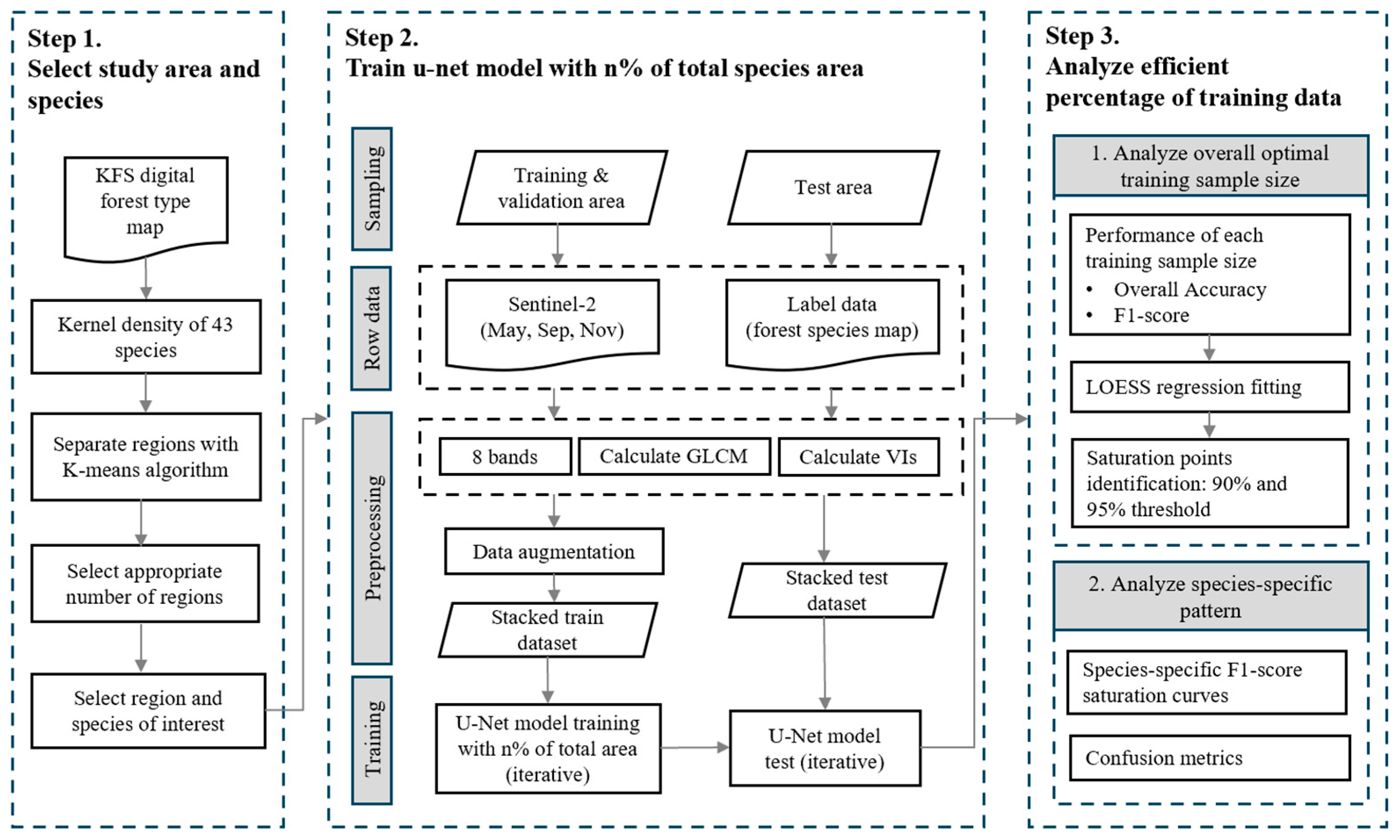
Figure 1. Research flow of this study.
Forests 16 01718 g001
Figure 2. Eight regions classified by kernel density for tree species (left) and spatial distribution of nine tree species in the Seoul–Gyeonggi region (right).
Forests 16 01718 g002
Figure 3. Training and test sample areas extracted from the Seoul–Gyeonggi region.
Forests 16 01718 g003
Figure 4. U-Net architecture for tree species classification. Each blue box represents a feature map layer with numbers above indicating channels and spatial dimensions shown below. Purple boxes denote encoder feature maps transferred via skip connections and concatenated with decoder features. Different operations are indicated by arrows and symbols as shown in the legend. The model takes 66-channel input and produces 10-class output through symmetric encoder–decoder paths with skip connections. Modified from Ronneberger et al. [41].
Forests 16 01718 g004
Figure 5. Model performance metrics as a function of training sample size. OA and F1-score with LOESS regression curves (span = 0.6). Shaded areas represent 95% confidence intervals of the fitted curves. Vertical dashed lines indicate the 90% optimal points of maximum performance, and solid lines indicate the 95% optimal points.
Forests 16 01718 g005
Figure 6. Species-specific F1-score performance curves as a function of training sample size. Each panel displays the performance trajectory for individual forest species, accompanied by LOESS regression curves (span = 0.6). Shaded areas represent 95% confidence intervals. Vertical dashed lines indicate 90% and solid lines indicate 95% of maximum performance for each species.
Forests 16 01718 g006
Figure 7. Confusion matrix for the best-performing model (random seed = 42, training sample size of 24.04%). Values represent the proportion of reference pixels (rows) classified as predicted species (columns). Diagonal values indicate correct classification rates for each species.
Forests 16 01718 g007
Figure 8. Relationship between training sample size and F1 score for nine tree species (random seed = 42, training sample size of 24.04%).
Forests 16 01718 g008
Table 1. Precision, recall, and F1-score for nine tree species classification (random seed = 42, training sample size of 24.04%). Values in parentheses represent 95% confidence intervals.
SpeciesPrecisionRecallF1-Score
Pinus rigida0.72 (0.720–0.723)0.57 (0.567–0.571)0.64 (0.635–0.638)
Larix kaempferi0.74 (0.736–0.740)0.64 (0.637–0.641)0.69 (0.683–0.686)
Pinus densiflora0.56 (0.554–0.559)0.54 (0.539–0.543)0.55 (0.547–0.551)
Pinus koraiensis0.71 (0.709–0.712)0.77 (0.771–0.774)0.74 (0.739–0.742)
Quercus acutissima0.41 (0.407–0.412)0.48 (0.475–0.481)0.44 (0.439–0.444)
Robinia pseudoacacia0.36 (0.358–0.365)0.42 (0.418–0.426)0.39 (0.387–0.393)
Quercus variabilis0.46 (0.460–0.464)0.60 (0.598–0.603)0.52 (0.520–0.524)
Quercus mongolica0.56 (0.552–0.557)0.75 (0.747–0.752)0.64 (0.635–0.640)
Castanea crenata0.63 (0.620–0.630)0.40 (0.391–0.399)0.48 (0.480–0.488)
Disclaimer/Publisher’s Note: The statements, opinions and data contained in all publications are solely those of the individual author(s) and contributor(s) and not of MDPI and/or the editor(s). MDPI and/or the editor(s) disclaim responsibility for any injury to people or property resulting from any ideas, methods, instructions or products referred to in the content.