Elevational Patterns of Plant Species Richness: Insights from Western Himalayas

Abstract

Understanding the patterns and drivers of species distribution has remained a central theme for biogeographical, conservation, and ecological research. This study aims to investigate the elevational patterns of plant species richness and compare the observed species richness with the predictions of the mid-domain effect (MDE) null model. By combining information from field observations and the published literature, we compiled a comprehensive database of the elevational distribution of plant species for three protected areas in the Western Himalayas. We used generalised linear model (GLM) and null model simulations to explore the elevational patterns of plant species richness. Our study revealed simple linear to complex non-linear patterns depending on the location and range of the elevational gradient. While non-linear unimodal patterns were common, a linear decreasing pattern was also observed. The observed species richness showed consistent deviations from the predictions of the mid-domain effect null model, suggesting that factors beyond the range constraints shape species richness patterns. These observations indicate that richness patterns are not solely generated by random processes, rather climatic gradients, ecological interactions, and topographic heterogeneity can shape these patterns. Understanding these factors can aid in predicting and managing the impacts of ongoing environmental changes on Himalayan biodiversity.

1. Introduction

More than two million living species have been scientifically documented and many more are yet to be discovered [1]. This enormous biodiversity is unevenly distributed on the planet and mountains harbour an unusually higher number of species than any other terrestrial region [2]. Even within mountain ranges, species number shows striking variation as one moves from valleys to mountaintops [3,4]. The change in the number and diversity of species along an elevation gradient is referred to as elevational patterns of species richness, which show how species richness varies as one moves up or down a mountain or hillside. This field of research investigates the patterns and environmental drivers of changes in species richness across elevational gradients. The distribution of species along elevational gradients has long intrigued ecologists [5] and remains a topic of active research in the fields of biogeography, conservation, and ecology [3,4,5]. Understanding these patterns is essential for unravelling the factors that shape biodiversity and ecological processes in different ecosystems. It is a pre-requisite for identifying high-diversity areas and has important implications for the conservation and sustainability of fragile mountain ecosystems like the Himalayas. Also, studying elevational patterns can inform conservation strategies in the face of ongoing environmental changes, such as climate change, which are expected to profoundly affect mountain ecosystems [2,6].

For a long time, it was believed that elevational gradients are mere reflections of latitudinal gradients [7,8] and the number of species (species richness) decreases monotonically towards mountain tops [4,5]. However, this decreasing pattern was challenged during the late 20th century and a unimodal (hump-shaped) pattern was suggested to be more common than the monotonic decline [4,9]. During the past few decades, numerous studies investigated the elevational patterns of species richness for different taxa and diverse mountain ranges [3,4,10]. These studies documented elevational patterns for bacteria [11], birds [12], bryophytes [13,14], pteridophytes [15,16,17,18], gymnosperms, angiosperms [19], vascular plants [20,21,22], trees [23,24], orchids [25], and other multiple taxa [26]. Across global mountains, these studies investigated elevational patterns for mountains of the central Balkans of Serbia [25], Crete [21], Ecuador [24], Himalayas [15,27,28,29], Mediterranean mountains [30], Myanmar [17,19], Mount Kilimanjaro of East Africa [26], Nepal [13,22,31], Panama [14], and the Rocky Mountains of Colorado [11].

The growing body of the literature suggests that the elevational patterns of species richness can be categorised into six major types: (i) unimodal, (ii) unimodal–decreasing, (iii) decreasing, (iv) unimodal–increasing, (v) increasing, and other [3,4,10,20]. These studies frequently documented a unimodal relationship, though some studies observed a decreasing pattern [19,21,27], a plateau [16], or even an increase [16,22] in species richness with elevation. The unimodal pattern is repeatedly reported from tropical and subtropical ecosystems, whereas the decreasing patterns are more common in temperate ecosystems [3,4,10]. Further, the unimodal pattern has been observed for a range of taxa, including plants [3,9,10]. However, birds [12] and ferns [16,17] showed highly variable patterns of elevational species richness. These variations indicate that the elevational patterns are not fully documented and understood yet [3,5].

While multiple biological, ecological, and historical processes can shape the elevational patterns of species richness [10,32,33], simple geometric constraints can also produce a unimodal pattern of species richness [34,35]. If random species with varying distribution ranges are placed in bounded domains, more species will overlap near the domains’ centre than the edges. Thus, a unimodal pattern of species richness can be achieved solely due to the random placement of species ranges [34]. This observation of richness peaks at intermediate elevations simply due to geometric constraints has been referred to as the mid-domain effect (MDE). The prediction of the MDE has been used as a null model because it operates solely due to random processes and does not consider any abiotic or biotic gradient [22,35]. The MDE null model assumes that species ranges are randomly distributed within the given domains, and predicts a unimodal pattern of species richness along an elevational gradient, with peak richness occurring at the midpoint of the gradient. This pattern arises due to the geometric constraints imposed by the boundaries of the elevational range [35]. Thus, the MDE model assumes that species richness is solely determined by the spatial constraints of the geographic range, independent of environmental factors [34]. The available literature indicates variable agreement between observed species richness and the MDE predictions [35,36], suggesting the influence of factors other than range constants in shaping the elevational patterns of species richness.

Despite the growing literature on elevational patterns, our knowledge remained limited. Firstly, the observed richness patterns seem to depend on the regional biogeographic context, taxonomic scope, and methodological approaches [10]. Secondly, available global syntheses highlight strong regional variation, but comparative datasets remain geographically biased towards Europe and the Americas, with underrepresentation of Asia and Africa [3,4,10]. Therefore, the investigating elevational patterns for multiple taxa across different biogeographic regions will be valuable. Thirdly, the observed species richness patterns can be influenced by the range and location of the elevational gradients, and the number of observed species. However, such aspects of methodological issues remained poorly investigated [37]. Fourthly, the observed unimodal patterns of species richness can be solely generated due to random processes. However, the contribution of these random processes remained debated. Therefore, comparing the observed richness patterns to the predictions of some null models will be insightful. These perspectives have been tested in mountain systems worldwide, yet their relative importance remains debated.

In the Himalayas, studies in central and eastern regions have shown both unimodal and monotonic patterns of plant richness [13,15,18,22,31,38], but equivalent analyses in the Western Himalayas remained limited [27,39,40]. Our study addresses this gap by compiling a comprehensive species database across three protected areas and explicitly comparing the observed elevational patterns with the predictions from the MDE null model. Specifically, the present study aims to (1) compare the plant species richness among different sites, (2) investigate the patterns of plant species richness across different elevational gradients, (3) compare the observed species richness with the predictions of the mid-domain effect null model across different elevational gradients, and (4) explore the elevational pattern of residual species richness (observed–predicted species richness). Our findings will contribute to enhancing our understanding of the elevational patterns of plant species richness. Further, this knowledge can inform conservation and management efforts and help us predict how plant communities will respond to future climate change.

2. Methodology

2.1. Study Sites

The Western Himalayas represent the prominent mountain ranges spanning Jammu and Kashmir, Himachal Pradesh, Uttarakhand, and parts of Punjab and Haryana in India. The present study focused on protected areas (wildlife sanctuaries) and their adjoining forested landscapes within the Western Himalayas. Specifically, we selected the Morni Hills (including Khol Hi-Raitan Wildlife Sanctuary), Chail Wildlife Sanctuary, and Churdhar Wildlife Sanctuary of the Western Himalayas based on their ecological significance and accessibility. The Morni Hills (300–1500 m) is located in the Panchkula district of Haryana, the Chail WLS (900–2100 m) is shared by the Solan and Shimla district of Himachal Pradesh, and the Churdhar WLS (1600–3600 m) is shared by the Sirmaur and Shimla districts of Himachal Pradesh (Figure 1). These three sites provided a broader elevational gradient ranging from 300 m in the lower foothills to over 3600 m at the Churdhar Peak. These sites’ diverse ecological zones and topographic variation offered us an ideal setting to investigate the elevational patterns of plant species richness in the Western Himalayas.

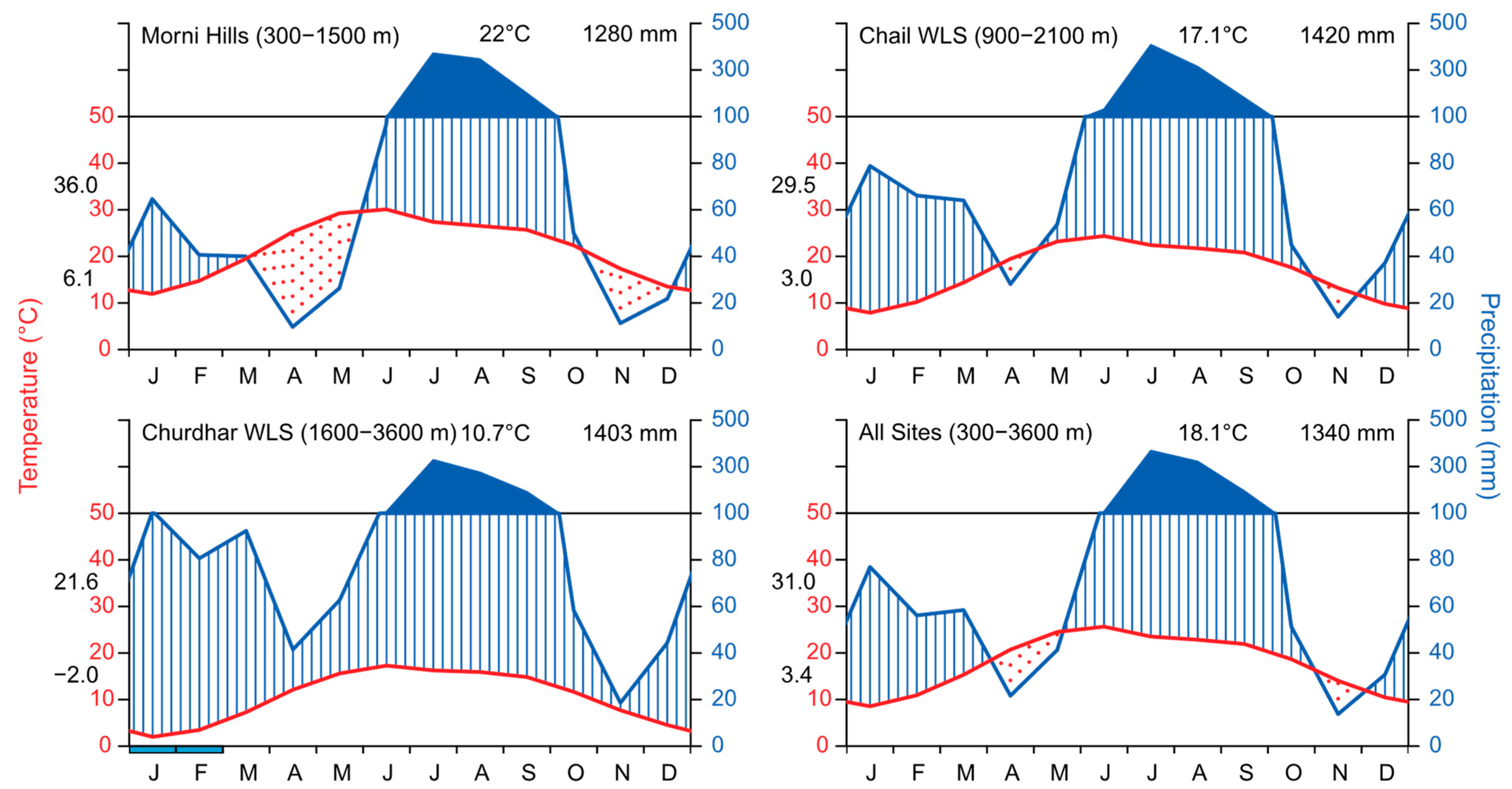
The selected study areas exhibit substantial variations in climate conditions due to significant variations in elevation and topography (Figure 2). Generally, the climate can be divided into three seasons, i.e., summer, monsoon, and winter. The climate varies from hot semi-arid (BSh) at the foothills to monsoonal warm-summer humid continental climate (Dwb) near Chur Peak. The Morni Hills represents the hot semi-arid (BSh) to monsoonal dry-winter humid subtropical climates (Cwa), the Chail WLS represents the monsoonal humid subtropical climate (Cwa) to monsoonal dry-winter subtropical highland climate (Cwb), and the Churdhar WLS represents the monsoonal dry-winter subtropical highland climate (Cwb) to monsoonal warm-summer humid continental climate (Dwb) near the Chur Peak [41].

The Morni Hills (300–1500 m) harbours the tropical mixed dry deciduous forests at lower elevations and Siwalik Chir Pine forests at higher elevations. The Chail WLS (900–2100 m) comprises subtropical Pine forests at lower elevations, followed by oak forests and moist Deodar forests at higher elevations with the occasional presence of Blue Pines. The Churdhar WLS (1600–3600) encompasses mixed coniferous forests at lower elevations, followed by Kharsu Oak forests and alpine pastures at higher elevations [42]. Thus, these sites represent diverse plant communities, ranging from temperate forests of oak and rhododendron to alpine meadows adorned with vibrant wild-flowers. These diverse forests are home to some Endangered (Aconitum heterophyllum Wall. ex Royle, Angelica glauca Edgew., Cypripedium himalaicum Rolfe, Dactylorhiza hatagirea (D.Don) Soó, Picrorhiza kurroa Royle ex Benth., Taxus wallichiana Zucc., and Trillium govanianum Wall. ex D.Don), Vulnerable (Cypripedium cordigerum D.Don, Malaxis muscifera (Lindl.) Kuntze, and Paris polyphylla Sm.), and Near Threatened (Abies spectabilis (D.Don) Mirb.) vascular plants according to the recent assessment [43]. Similarly, numerous endemic wild animals like Himalayan musk deer and Himalayan brown bears thrive in the study areas. The Chail WLS and Churdhar WLS are included in the Important Bird and Biodiversity Areas of BirdLife International [44] and provide a home to some threatened birds including the Cheer Pheasant (Catreus wallichii Hardwicke, 1827), Himalayan Monal (Lophophorus impejanus Latham, 1790), Indian Vulture (Gyps indicus Scopoli, 1786), Koklass Pheasant (Pucrasia macrolopha Lesson, 1829), Red-headed Vulture (Sarcogyps calvus Scopoli, 1786), and White-rumped Vulture (Gyps bengalensis Gmelin, JF, 1788).

Figure 2. Walter and Lieth [45] climate diagrams for Morni Hills (top-left), Chail WLS (top-right), Churdhar WLS (bottom-left), and All Sites (bottom-right) showing the variation in average monthly temperature (shown in red) and precipitation (shown in blue) for 1970 to 2000. The text in the (top-left) corner of each plot represents the name of the site with its elevation range in parenthesis and the period for which climate data is represented. Similarly, the text in the (top-right) corner of each plot shows the mean annual temperature (°C) and mean annual precipitation (mm). The x-axis denotes the months and likely frost months are filled with sky blue. The left y-axis represents the temperature in °C (with red text), whereas the right y-axis depicts the precipitation in mm (with blue text). The minimum average temperature of the coldest month and maximum average temperature of the hottest month are represented on the left y-axis with black text. Above 100 mm precipitation, the scale of the right y-axis is increased from 2 mm/°C to 20 mm/°C and this change in scale is marked by the black horizontal line in each plot. The area filled with red dots represents the dry period where the precipitation curve falls below the temperature curve. Similarly, the area filled with blue vertical lines shows the humid period where the precipitation curve falls above the temperature curve. The area filled in solid blue indicates the wet period where the precipitation curve falls above the black horizontal line, representing the precipitation above 100 mm. The climate data was accessed from WorldClim database [46].

Figure 2. Walter and Lieth [45] climate diagrams for Morni Hills (top-left), Chail WLS (top-right), Churdhar WLS (bottom-left), and All Sites (bottom-right) showing the variation in average monthly temperature (shown in red) and precipitation (shown in blue) for 1970 to 2000. The text in the (top-left) corner of each plot represents the name of the site with its elevation range in parenthesis and the period for which climate data is represented. Similarly, the text in the (top-right) corner of each plot shows the mean annual temperature (°C) and mean annual precipitation (mm). The x-axis denotes the months and likely frost months are filled with sky blue. The left y-axis represents the temperature in °C (with red text), whereas the right y-axis depicts the precipitation in mm (with blue text). The minimum average temperature of the coldest month and maximum average temperature of the hottest month are represented on the left y-axis with black text. Above 100 mm precipitation, the scale of the right y-axis is increased from 2 mm/°C to 20 mm/°C and this change in scale is marked by the black horizontal line in each plot. The area filled with red dots represents the dry period where the precipitation curve falls below the temperature curve. Similarly, the area filled with blue vertical lines shows the humid period where the precipitation curve falls above the temperature curve. The area filled in solid blue indicates the wet period where the precipitation curve falls above the black horizontal line, representing the precipitation above 100 mm. The climate data was accessed from WorldClim database [46].

2.2. Species Check-List

A comprehensive species check-list was compiled for each site by combining the information gathered from field surveys and literature surveys. We conducted 2–4 field visits of each site during 2018–2022 in pre-monsoon (March to July) and post-monsoon (September to November) seasons. We recorded the identifiable plant species encountered on the treks followed by us. Unknown plants were photographed and identified in the lab with the help of the literature and the herbarium (PAN) of the Panjab University, Chandigarh, and the Janaki Ammal Herbarium (RRLH) of the Indian Institute of Integrative Medicine, Jammu. On-line resources like eFlora of India and Flowers of India were also consulted for plant species identification [47,48]. Further, we conducted a systematic literature survey to identify the previously reported plant species from the selected sites following the earlier defined methodology [49]. Google Scholar was chosen for the identification of relevant studies for two reasons. Firstly, it can retrieve the most obscure sources, including studies published in local publication outlets and technical reports. Secondly, it can search within the full text of available articles. Considering these advantages, we searched Google Scholar using “Morni”, “Chail”, and “Churdhar” as keywords in September 2021 and the search was again updated in August 2022. We recorded all the plant species reported from the identified accessible studies for each selected site. To prepare a complete check-list of reported plant species for all the sites, we updated our check-list by adding plant species that were collected and reported by earlier studies for the Morni Hills [50,51,52,53,54], Chail Wildlife Sanctuary [55,56,57], and Churdhar Wildlife Sanctuary [58,59,60,61,62,63].

The World Checklist of Vascular Plants (WCVP) was followed to standardise all the botanical names and their authorities [64]. It is based on the International Plant Names Index (IPNI) and managed by the taxonomic experts at the Royal Botanic Gardens, Kew. It is considered superior to the traditionally used The Plant List (TPL v1.1) because it is expertly reviewed and most importantly, follows the International Code of Nomenclature [65]. Further, the WCVP follows the Angiosperm Phylogeny Group IV (APG IV) system of botanical classification [66]. The WCVP database is updated daily and is a taxonomic backbone for the Plants of the World Online [67]. We manually screened and standardised each record of plant species using the Plants of the World Online portal during 2021–2022 [67]. All records of taxonomic names were updated by assigning the recently accepted names, including the spelling variants and botanical authorities [67]. We generally accepted the infra-specific taxa (variety and subspecies) as species for the present analysis to maintain harmony among the taxa. Further, we recorded the distribution of each plant from the [67] and excluded all those taxa whose distribution was found outside of India for the Morni Hills and outside of Western Himalaya for the Chail WLS and Churdhar WLS. We manually corrected the known distribution of some species (Bauhinia variegata as Introduced to the Himalayas but Native to India). Recently, we updated the plant names and their families by matching them with a static copy of WCVP (version 10 dated 27 October 2022) using the package rWCVP version 1.2.4 [68].

2.3. Distribution Ranges

The elevational distribution of each catalogued species was recorded from the recently compiled Database of Vascular Plants of Himalaya published on GBIF [69,70]. This dataset comprises over 10,500 plant species compiled from published floras for the Himalayan region [69,70]. It included over 3300 plant species from Himachal Pradesh with elevational distribution for about 3000 species from the published floras [71,72,73]. We accessed this dataset on 6 August 2022 through GBIF using the package rgbif version 3.8.2 [74]. The plant names provided by the authors of this dataset were standardised by matching with a static copy of WCVP (version 10 dated 27 October 2022) using the package rWCVP version 1.2.4 [68]. We filtered the elevational distribution of plants in Himachal Pradesh and then joined these elevational distributions to our plant check-list. This procedure provided elevational distribution for more than 1000 plants. Similarly, elevational data for about ten species was extracted from another published study [75]. We excluded the remaining species (n = 228) whose elevational data was either unavailable or uncertain. Next, we manually screened the elevational data for each species. In the case of duplicates, we considered the maximum value for the upper limit and the minimum value for the lower limit [75]. Further, we preferred the data from Himachal Pradesh over the neighbouring states or the entire Himalayas because our sites broadly fall under this Indian state. However, some species had their elevational distribution extending beyond our sites’ elevational range (300–3600 m). Therefore, we adjusted the minimum lower limit of distribution to the minimum elevation of the study site, the minimum upper limit of distribution to the minimum elevation of the study site plus 100 m, and the maximum upper limit of distribution to the maximum elevation of the study site rounded to the nearest hundred. Thus, the elevational distribution limits represented ‘soft boundaries’ for each site [76].

2.4. Species Richness

We accessed the elevation data from the Amazon Web Services Terrain Tiles and the Open Topography global datasets API using the get_elev_raster() function from the elevatr package version 0.99.0 [77]. Then, we re-sampled the elevation to 30 arc-sec (~1 km) raster with bilinear interpolation using the resample() function from the terra package version 1.8.60 [78]. This re-sampling updated the elevational extents of the Morni Hills (300–1300 m), Chail WLS (900–2100 m), Churdhar WLS (1600–3400 m), and All Sites (300–3400 m). We divided each elevational gradient into 100 m elevational bands for each site to estimate species richness at different elevations. Such 100 m elevational bands have been previously used to study the elevational patterns of species richness in plants [18,29,75]. Thus, the species richness was estimated in 10 bands for the Morni Hills, 12 bands for the Chail WLS, 18 bands for the Churdhar WLS, and 31 bands for All Sites combined. Each elevational band is represented by the upper elevational limit in both text and figures.

We used the range interpolation approach to estimate the species richness for each elevational band, assuming that each species can be found everywhere between its elevational range [31]. The range interpolation method has been widely used to study the elevational patterns of plant species richness [37,75,79]. Although this approach can introduce bias in estimating species richness [37], it is commonly applied for compensating the sampling problems and overall methodological consistency. Therefore, we assigned each species to all elevational bands occurring wholly or partly within its known elevational range [18,31,75]. Then, the species richness was estimated as the total number of species present in each 100 m elevational band. Since this species richness corresponds to the whole elevational band, it represents the $\gamma$-diversity for each elevational band [5].

2.5. Data Analysis

Firstly, we aimed to compare species richness across different elevational gradients represented by our study sites. The number of unique and shared species among the study sites was summarised with a Venn diagram prepared using the ggVennDiagram package version 1.5.4 [80]. To compare the species richness across the study sites, we interpolated species richness with rarefaction to standardised sampling units and sample coverage [81,82,83,84]. This procedure allowed us to make a statistically fair comparison of richness and control for the differences in the elevational bands across the study sites [81]. Specifically, we estimated the expected species richness from the raw species-by-site incidence matrix and extrapolated to a maximum of 20 sampling units, i.e., number of elevational bands [81,82]. The mean, standard error, and 95% confidence intervals for species richness were estimated using bootstrap procedures (n = 100). The rarefaction analysis of species richness was implemented in the R statistical environment version 4.4.2 [85] using the iNEXT() function from the iNEXT package version 3.0.2 [86]. The differences in species richness were considered significant, if the estimated 95% confidence intervals did not overlap with each other [83].

Secondly, we aimed to explore the elevational patterns of plant species richness in the Western Himalayas. A generalised linear model (GLM) was used to examine the relationship between plant species richness as the response variable and elevation as the predictor variable. The GLM framework accommodates data with non-normal error distributions, models non-linear relationships, incorporates multiple predictors, and provides statistical inference [87]. Our response variable, plant species richness, was defined as the count of unique plant species observed within predefined elevation bands. We chose to use a Poisson distribution within the GLM due to the discrete and non-negative nature of our response variable. The Poisson distribution is commonly used when modelling count data, as it accounts for the inherent heterogeneity and overdispersion observed in such discrete data [87]. Therefore, we used the GLM framework with a Poisson distribution and logarithmic-link function, which ensures that the fitted values are always non-negative. The GLMs were implemented using the glm() function from the stats package in R programming environment version 4.4.2 [85].

We initially assessed the relationship between elevation and plant species richness using a scatter plot and calculated the Pearson’s correlation coefficient to explore the strength and direction of the association (Figure S1). To account for a unimodal or non-linear relationship between species richness and elevation [3,4], we included polynomial terms for elevation up to the fifth degree as predictors (Equation (1)).

$$S\sim Elev+Ele{v}^2+Ele{v}^3+Ele{v}^4+Ele{v}^5$$

(1)

We followed a forward model selection approach (Table S1) and evaluated a total of six models starting from an intercept-only null model (zero-degree) to a full model with fifth-degree polynomial elevation as predictor variables (Equation (1)). We measured the lack of fit of the model by calculating the deviance (D), which is the deviance of the fitted model from the perfectly saturated model (Table S1). A model’s deviance (D) is defined as twice the maximum log-likelihood ($\mathcal{L}$) of the model. Although there is no true $R^2$ statistic for GLMs, the pseudo-$R^2$ or the deviance-squared ($D^2$) of the model can be estimated by Equation (2):

$$D^2={\displaystyle \frac{D_{null}-D_{resid}}{D_{null}}}; D_{adj}^2=1-{\displaystyle \frac{\left(1-D^2\right)\times \left(n-1\right)}{n-k-1}}$$

(2)

where the $D_{null}$ is the deviance of the null model (model with only an intercept) and the $D_{resid}$ is the deviance of the model under study (saturated model). Thus, a smaller value of $D_{resid}$ will have higher explanatory power and, therefore, the model will be better. However, a smaller sample size can bias the deviance-squared; therefore, we adjusted the deviance-squared by applying a correction for a small sample size (Equation (2)). Additionally, we assessed the dispersion parameter ($\varphi$) since heterogeneous ecological data often has higher variance than the mean value of response (overdispersion), violating the assumption of Poisson GLM (Table S1). If there is overdispersion, then the quantity $D/\varphi$ will follow a ${\chi }^2$ distribution with $n-k$ degrees of freedom and the estimator for $\varphi$ will be the following:

$$\varphi ={\displaystyle \frac{D}{n-k}}$$

(3)

where $D$ is the residual deviance, $n$ is the total number of observations (sample size), and $k$ is the number of unknown parameters (predictors) in the fitted model. If the estimated values of $\varphi$ in Equation (3) are close to 1, we can assume there is little or no overdispersion [87].

We used the information theory-based model selection criteria to identify the best model from the candidate models (Table S1). Akaike’s Information Criterion (AIC) has been commonly used for model comparison in ecology and evolution [88]. However, it can bias model comparison when the sample size is small compared to the number of estimated parameters [89]. Therefore, we corrected the AIC by applying a sample size correction suggested by [90], which can be mathematically represented by Equation (4):

$$AIC=-2\mathcal{L}+2k; AICc=AIC+{\displaystyle \frac{2k\left(k+1\right)}{n-k-1}}$$

(4)

where $k$ is the number of parameters to be estimated by the model and $n$ is the total number of response observations in the model. The model with the lowest AICc value was considered the best and models with a difference of two AICc units were considered equally competitive [89]. Since our models are nested, we statistically compared the larger (more predictors) models with smaller (less predictors) models using a deviance-based Chi-squared test, also known as the likelihood ratio test (Table S1). A significant p-value (i.e., p < 0.05) suggests substantial improvement in model fit when additional predictors were included, i.e., the larger model is better than the smaller model.

Once the models were selected, a thorough evaluation of their performance was conducted to ensure the validity of the findings. Model evaluation involves assessing the assumptions of the selected models and diagnosing potential issues. We used simulated residuals (n = 1000) to visually determine the model fit by plotting residuals against the model predictions [91]. Then, the model was validated by analysing the dispersion and distributional assumptions of the fitted model. The simulated residuals from the defined distribution were tested against the residuals of the fitted model. Specifically, the uniformity was tested using the Kolmogorov–Smirnov (KS) test, dispersion was tested using the simulation-based dispersion test, and outliers were tested by generating a simulation-based expectation for the outliers using bootstrapping. If the dispersion test indicated significant over-/underdispersion, we assessed the variance in the observed raw residuals against the variance in the simulated residuals. The deviations in the model residuals were visually considered by plotting the simulation-based residuals against the model predictions. This residual analysis and model validation was implemented using the simulateResiduals() function from the DHARMa package version 0.4.7 [92]. Additionally, we performed the deviance-based Chi-squared goodness-of-fit test to assess the overall goodness of fit of the selected model. A non-significant p-value indicates that there is no significant difference between the predictions of the model and the observed data, i.e., the data is adequately fitted to the model. After assessing the goodness of fit for the selected models, we used Wald’s test to evaluate the significance of the estimated regression coefficients.

Our third aim was to compare the observed species richness with the predictions of a null model. A null model predicts the observed patterns solely due to the operation of random processes [93]. The geometric constraint hypothesis or the mid-domain effect is a commonly used null model to evaluate species richness patterns [31,76]. This hypothesis predicts that the species richness patterns emerge from a random distribution of species ranges. The elevational range of a species is defined as the difference between the highest and lowest elevation of its geographical distribution and the elevational midpoint as the mean of these two limits [8]. We randomly generated elevational ranges equal to the number of species in each site. The elevational ranges were generated by defining the geometric constraints of boundaries, i.e., the lower and upper elevational limits corresponding to each study site (Box 2 in Ref. [34]). These elevational limits were re-arranged so that the lower value should represent the lower limit, whereas the higher value should represent the upper limit of the elevational range. Then, the species richness was calculated by assuming that the species is continuously present within its elevational range. Next, we calculated the species richness in each 100 m elevational band starting from the minimum elevation to the maximum elevation. This process was repeated 10,000 times to estimate the minimum, maximum, mean species richness, and associated standard deviation for each elevational band. The mean species richness (S_null) predicted by this null model was compared with the observed species richness (S). We used linear regression analysis to compare the strength of the association between the observed species richness and predictions of the null models. If the observed species richness is well agreed with the predictions of the null model, then the slope value should be close to one.

Fourthly, we estimated the residual species richness (S_res), representing the difference between the observed (S) and predicted species richness (S_null) for each 100 m elevational band. The residual species richness (S_res) was calculated by subtracting the predicted species richness (generated by the mid-domain effect null model) from the observed species richness for each 100 m elevational band. Positive residuals indicated higher species richness than expected, while negative residuals indicated lower species richness than expected. We initially assessed the relationship between elevation and residual species richness using a scatter plot and calculated the Pearson’s correlation coefficient to explore the strength and direction of the association (Figure S2). We included quadratic and cubic elevation terms as predictors to account for the non-linear relationship between residual species richness and elevation. Then, we used polynomial linear regression to analyse the elevational pattern of residual species richness (S_res). The goodness of fit for the polynomial models was assessed using the adjusted coefficient of determination (R²_adj), with higher values indicating better model fit. The significance of the estimated regression coefficients was determined using the t-test and p-values less than 0.05 were considered significant.

Finally, we tested the effect of the total number of observed species (N_obs) on the elevational patterns of plant species richness. We re-calculated the species richness for each 100 m elevational band at different levels of the total number of species by randomly removing and adding 50 to 200 species to the total number of observed species for each site. To test the effect of further additions to the total observed species, we re-calculated species richness by adding randomly sampled elevational ranges for 50, 100, 150, and 200 virtual species. Similarly, we tested this effect in the reverse direction by randomly removing 50, 100, 150, and 200 observed species. Thus, we estimated species richness at nine levels (−200, −150, −100, −50, 0, 50, 100, 150, and 200) of the total number of observed species for each site. Further, we calculated the predicted species richness from the mid-domain effect null model (S_null) for these nine levels of the total species for each site. Then, we used linear regression analysis to measure the relationship between the observed species richness and predicted species richness for different levels of the total number of species. Specifically, we estimated the slope value by regressing the observed species richness (S) against the predictions of the null model (S_null) using the general linear model for different levels of total species for each site. Next, we used the Pearson’s correlation coefficient (r) to test how the total number of species (N_obs) affects the relationship between the observed species richness (S) and the predictions of the mid-domain effect null model (S_null). All analyses were implemented in R statistical environment version 4.4.2 [85] and the package tidyverse version 2.0.0 was used for general data wrangling and visualisation [94].

3. Results

3.1. Species Richness Across Sites

Our initial check-list included over 2500 records of plant species across the selected sites. The standardisation of botanical names revealed that over 1000 botanical names were synonyms and we were left with about 1400 unique botanical names. Further, screening for distribution showed that only 1385 were found within the study sites. These 1385 species belonged to 748 genera and 145 families (

Table 1. Summary of recorded vascular plant taxa from Morni Hills, Chail WLS, and Churdhar WLS.

Taxa	Morni	Chail	Churdhar	Total
Species	696	438	616	1385
Genus	471	322	346	748
Family	109	106	99	145
Introduced	120	45	16	142
Native	576	393	600	1243

The table includes the counts of unique taxa observed in each site, and the total number of unique taxa across all three sites. The taxa are categorised based on their taxonomic levels (species, genus, and family) and nativity (Introduced and Native).

).

According to the POWO distribution [67], 1243 species were found to be Native, whereas 142 species were Introduced to the region. The distribution of the three species differed between India and the Western Himalayas. For example, Bauhinia variegata L. and Impatiens balsamina L. are Native to India, but the distribution of the former is Doubtful or Introduced, whereas that of the latter is Introduced in the Western Himalayas. Similarly, Lysimachia arvensis (L.) U.Manns & Anderb. is Native to the Western Himalayas but Introduced in India.

A total of 696 species belonging to 471 genera and 109 families were recorded from the Morni Hills. Among these 696 species, 576 species were Native and 120 species were Introduced. In the Chail WLS, 438 species belonging to 322 genera and 109 families were recorded. Among these 438 species, 393 species were Native and 45 species were Introduced. The Churdhar WLS represented 616 species belonging to 346 genera and 99 families. Out of 616 species, this region had 600 Native and 16 Introduced species. Among all the selected sites, the Morni Hills recorded the maximum number of species, followed by the Churdhar WLS and Chail WLS (Table 1). Similarly, the number of Introduced species was maximum in the Morni Hills, whereas it was minimum in the Churdhar WLS.

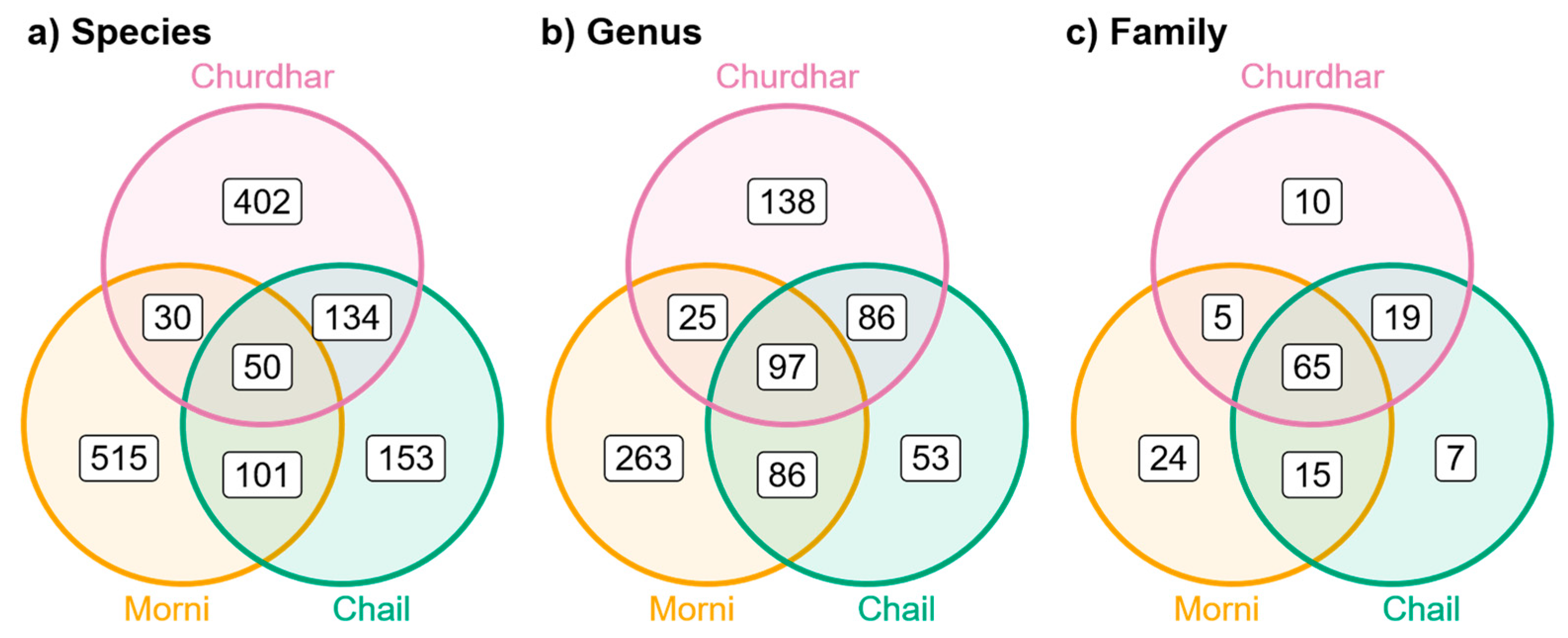
Out of 1385 species, 50 species were recorded from all the sites. The Morni Hills, Chail WLS, and Churdhar WLS had 515, 153, and 402 unique species, respectively. The Chail WLS and Churdhar WLS shared the highest number of plant species (n = 134), whereas the minimum species (n = 30) were shared by the Morni Hills and Churdhar WLS (Figure 3a). Similarly, about 97 genera were common to All Sites and the Morni Hills comprised the greatest number of unique plant genera (n = 263) followed by the Churdhar WLS (n = 138), whereas the Chail WLS had the lowest number of unique genera (n = 53). The Chail WLS shared the highest number of genera (n = 86) with the Morni Hills and Churdhar WLS, whereas only 25 were shared by the Morni Hills and Churdhar WLS (Figure 3b).

Taxa from 65 families were common to all the sites and the Morni Hills represents the highest number of unique families (Figure 3c). The Morni Hills, Chail WLS, and Churdhar WLS represented taxa from 24, 7, and 10 families, respectively. Generally, there was high similarity in taxa for the Chail WLS and Churdhar WLS, whereas the Morni Hills and Churdhar WLS exhibited unique taxonomic compositions of plants. Among the families of the recorded species (Table S2), Fabaceae was the most dominant with 133 species across All Sites, followed by Asteraceae (n = 109), Poaceae (n = 93), Lamiaceae (n = 58), and Rosaceae (n = 43).

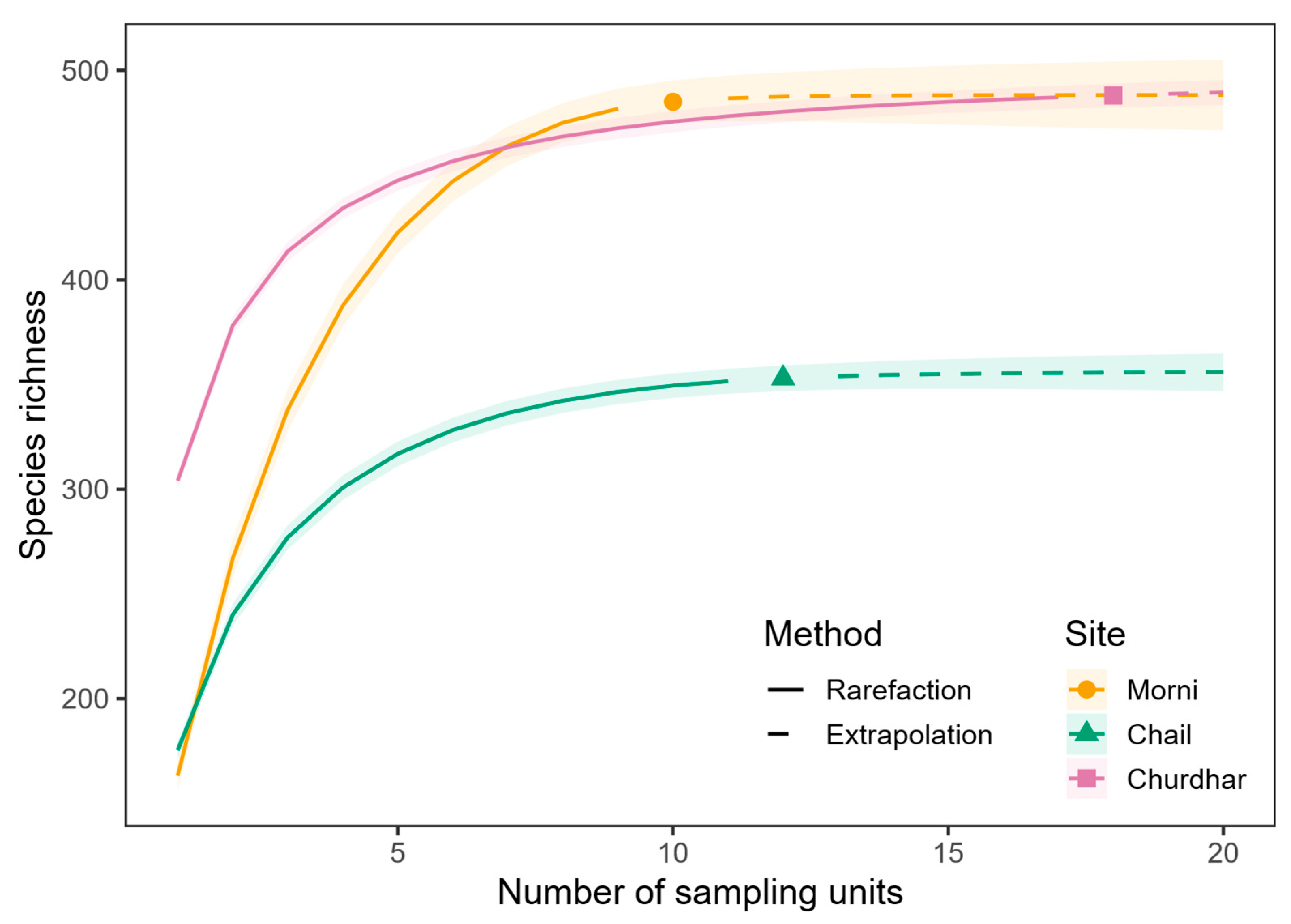
Further, we observed significant differences in plant species richness across the study sites along the elevational gradients (Figure 4). The estimated species richness was highest for the Morni Hills (mean = 485, 95% CI = 475–495), followed by the Churdhar WLS (mean = 476, 95% CI = 470–480) and it was lowest for the Chail WLS (mean = 349, 95% CI = 344–355) standardised at 10 sampling units, i.e., number of 100 m elevational bands. The 95% confidence intervals revealed that the species richness was significantly lower in the Chail WLS as compared to the Morni Hills and Churdhar WLS. However, the species richness was not significantly differed between the Morni Hills and Churdhar WLS (Figure 4). These results were also supported by the sample coverage-based rarefaction and extrapolation curves (Figure S3).

3.2. Elevational Patterns of Species Richness

We could not retrieve elevational data for all recorded species and, therefore, limited further analysis to only those whose distribution data was available. Thus, our analyses were based on a total of 1159 species from All Sites, including 568 from the Morni Hills, 377 from the Chail WLS, and 561 from the Churdhar WLS. Out of the six evaluated candidate models for each site (Table S1), the quadratic model was considered the best for the Chail WLS and Churdhar WLS to describe the elevational patterns. The cubic model was chosen for the Morni Hills, whereas the quartic (fourth-degree polynomial) model was selected for combined All Sites. Although the quadratic and cubic models were equally competitive for the Morni Hills, we selected the cubic model because it indicated better goodness of fit regarding the dispersion and residual diagnostics. Similarly, the quadratic model was chosen over the cubic model for the Churdhar WLS due to better model diagnostics for the quadratic model than the cubic model (Table S1). These selected models exhibited a good fit to the data as indicated by the goodness-of-fit measures (

Table 2. Summary of selected models to explain elevational patterns of species richness for each site.

Site	Model	D2	D2adj	$\mathit{\varphi }$	AICc	Dresid	dfresid	p
Morni	S ~ Elev + Elev2 + Elev3	0.97	0.94	1.07	91.00	6.39	6	0.381
Chail	S ~ Elev + Elev2	0.91	0.88	0.57	98.39	5.11	9	0.824
Churdhar	S ~ Elev + Elev2	0.98	0.98	0.94	156.64	14.06	15	0.521
All	S ~ Elev + Elev2 + Elev3 + Elev4	1.00	1.00	0.36	257.54	9.42	26	0.999

The plant species richness (S) was used as the response variable and elevation (Elev) as the predictor variable. Each model represents a generalised linear model (GLM) fitted using a Poisson distribution with the log-link function. The table presents the deviance explained (D²), adjusted deviance explained (D²_adj), dispersion parameter ($\varphi$), and corrected Akaike’s Information Criterion (AICc) for each model. The goodness of fit for each model was evaluated using a deviance-based Chi-squared goodness-of-fit test and the deviance (D_resid), degrees of freedom (df_resid), and associated p-values (p) are also reported.

). The quadratic, cubic, and quartic models explained over 90% of the total deviance for the selected sites. Additionally, the inspection of the model residuals also suggested an adequate model fit as indicated by the QQ plots (Figure S4) with the associated distribution tests and the residual plots to assess the deviation from the distribution assumptions (Figure S5). Although a significant underdispersion was observed for the All Sites data, the variance in the model residuals was not too large compared to that of the simulated residuals (Figure S6).

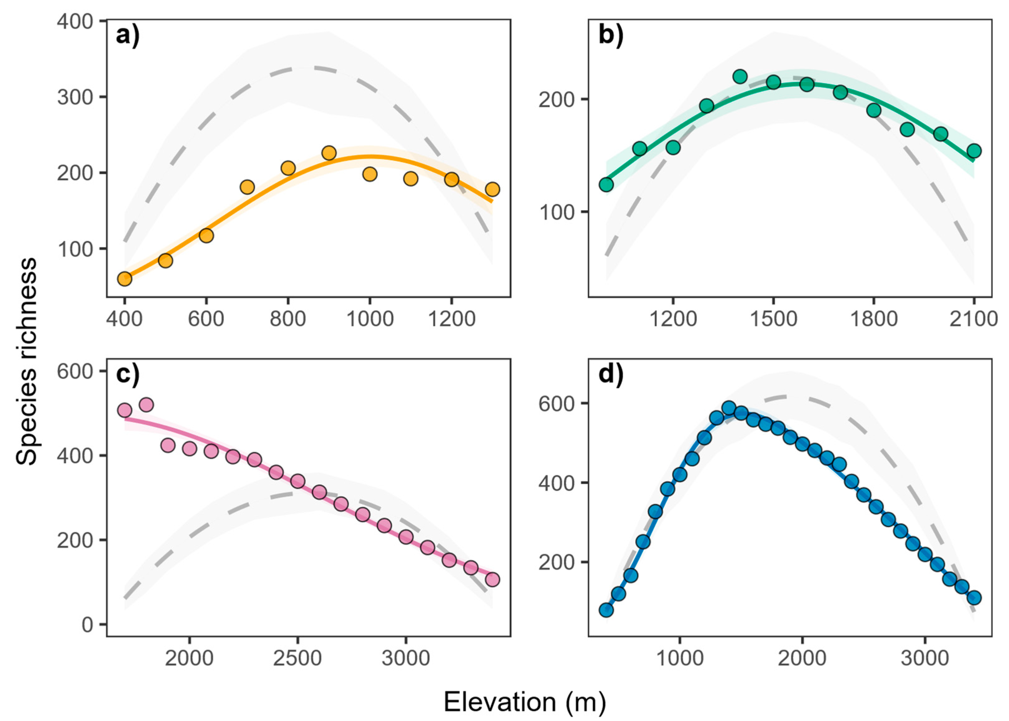
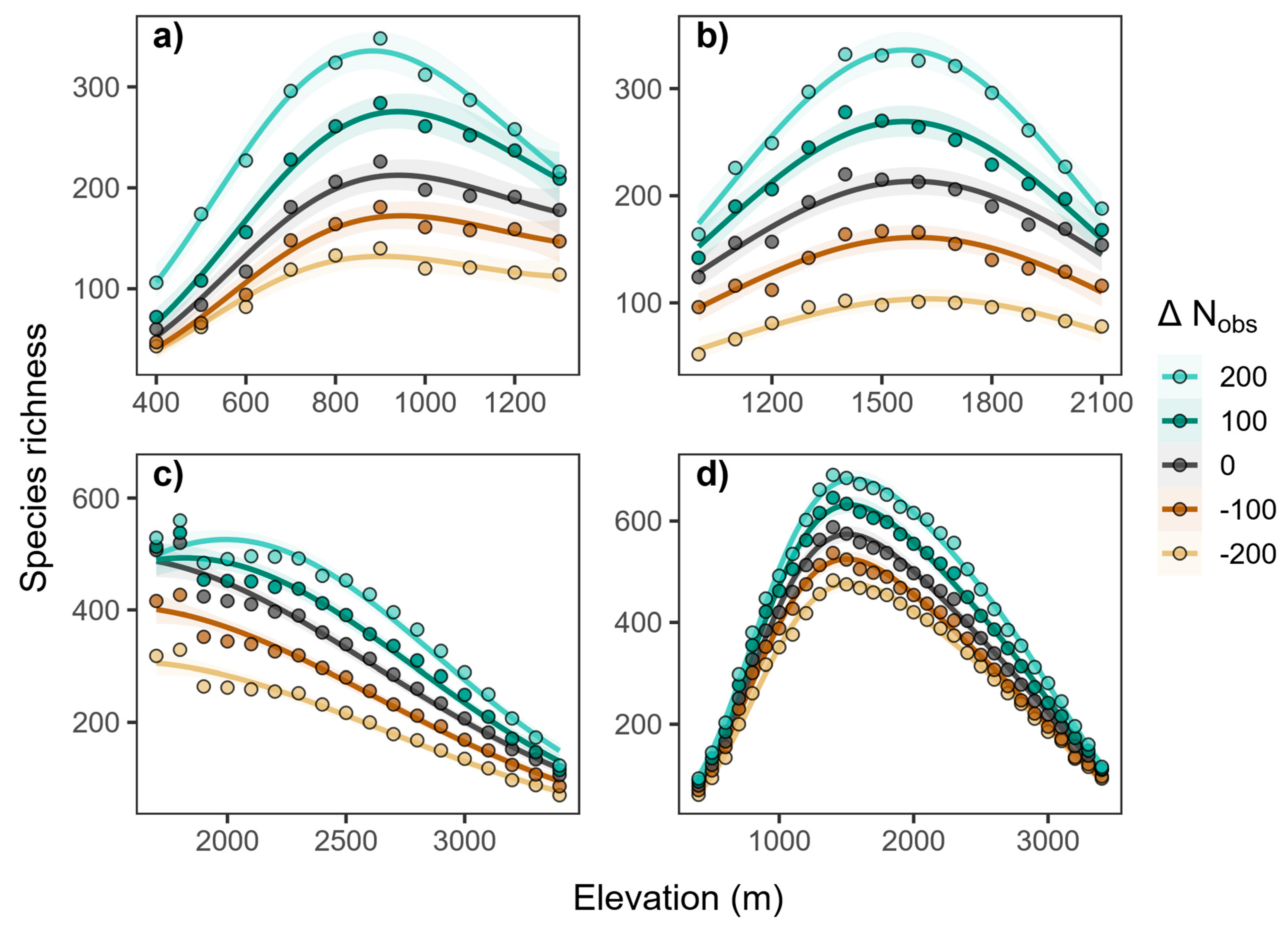
The species richness varied from 60 to 226 in the Morni Hills, 124 to 220 in the Chail WLS, 106 to 520 in the Churdhar WLS, and 79 to 588 across All Sites. The elevational patterns of plant species richness also differed among the selected sites. The elevational pattern of species richness followed a non-linear unimodal pattern for the Morni Hills, Chail WLS, and All Sites combined (Figure 5). This pattern showed an initial increase in plant species richness with the increasing elevation, reaching a peak and declining gradually at higher elevations. The species richness peaked around 800–900 m in the Morni Hills, 1300–1400 m in the Chail WLS, and 1300–1400 m in All Sites. However, the Churdhar WLS showed a decreasing elevational pattern of plant species richness and the richness peak was observed around 1700–1800 in the Churdhar WLS (Figure 5c).

Wald’s test suggested that elevation is indeed significantly associated with species richness. All estimated coefficients differed significantly from zero, except the Intercept for the Morni Hills (

Table 3. Summary of estimated coefficients (mean ± SE) from polynomial regression analysis of elevational patterns of plant species richness.

Site	Intercept	Elev	Elev2	Elev3	Elev4
Morni	−0.15 ± 0.92	14.95 ± 3.46 ***	−13.1 ± 4.12 **	3.65 ± 1.56 *	NA
Chail	1.65 ± 0.51 **	4.68 ± 0.67 ***	−1.47 ± 0.21 ***	NA	NA
Churdhar	5.32 ± 0.36 ***	1.19 ± 0.3 ***	−0.4 ± 0.06 ***	NA	NA
All	1.8 ± 0.23 ***	8.49 ± 0.61 ***	−5.69 ± 0.56 ***	1.65 ± 0.21 ***	−0.19 ± 0.03 ***

The generalised linear model (GLM) was fitted by specifying the Poisson distribution with the log-link function. The species richness was used as the response variable and elevation (Elev) as the predictor variable. The significance of estimated coefficients was determined with Wald’s test and the significance levels ***, **, and * correspond to the p-value of <0.001, <0.01, and <0.05, respectively. The elevation was transformed into kilometre units before modelling.

). The linear and cubic elevation terms were positively associated, whereas the quadratic and quartic elevation terms were negatively associated with species richness. The coefficient for linear elevation (Elev) was positive and highly significant for all the selected sites. However, the magnitude was highest for the Morni Hills and lowest for the Churdhar WLS, suggesting that the increase in species richness is expected to be higher in the Morni Hills than in the Churdhar WLS (Table 3). Similarly, the coefficient for quadratic elevation (Elev²) was negative and highly significant for all the sites, suggesting a significant decrease in species richness at higher elevations. The Chail WLS and Churdhar WLS included only quadratic elevation terms, suggesting that the pattern does not exhibit significant non-linear patterns beyond the quadratic term. However, the Morni Hills included a significant cubic elevation (Elev³) and All Sites quartic elevation (Elev⁴), suggesting a significant non-linear relationship between elevation and species richness.

3.3. Comparison with the Null Model

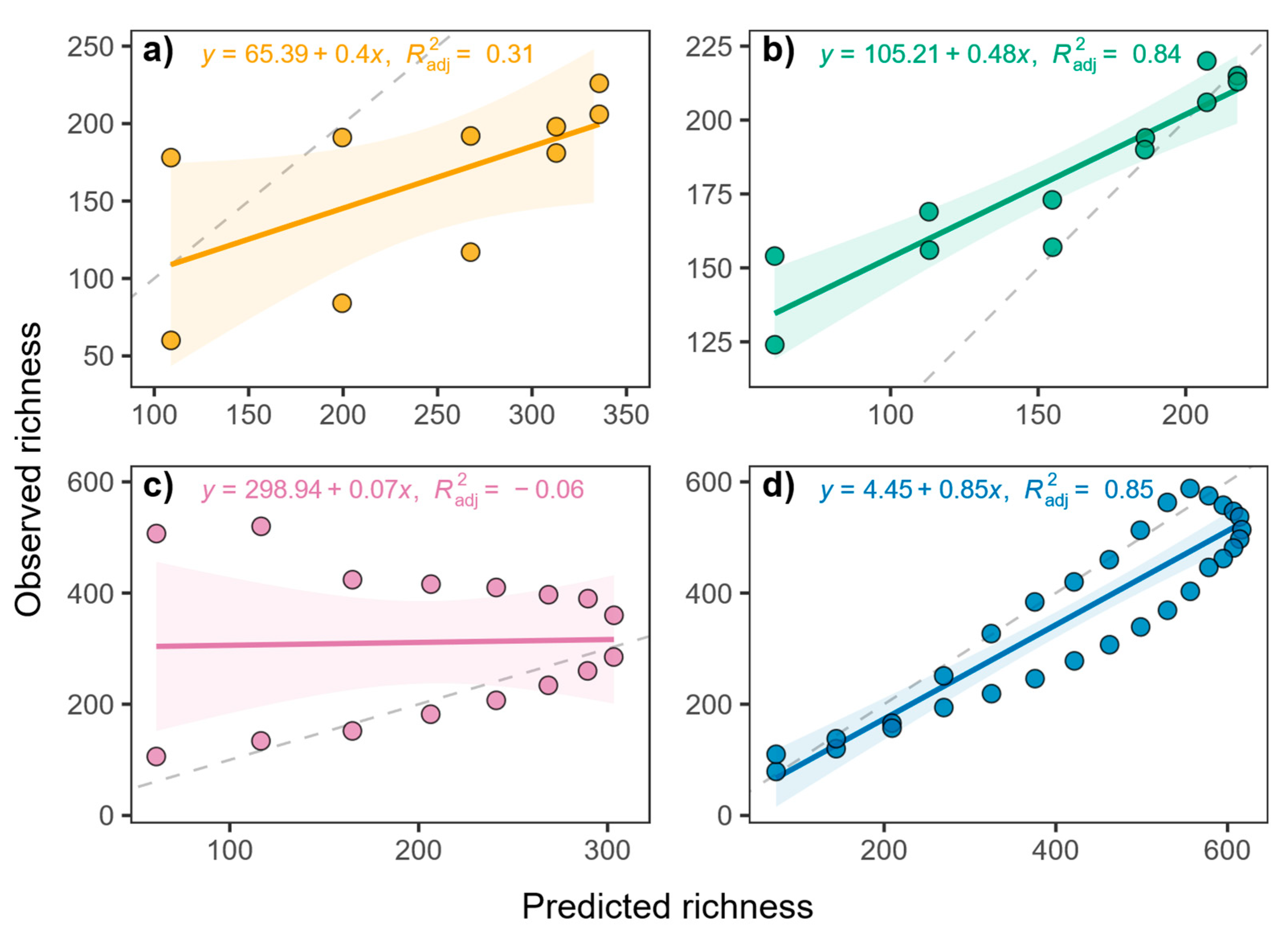
The comparison of the observed species richness (S) with the predicted species richness (S_null) from the mid-domain effect null model indicated substantial deviations (Figure 6). The results of the simple linear regression showed that the null species richness (S_null) did not fully explain the observed species richness (Table S3). The null species richness is significantly and positively associated with the observed species richness for the Chail WLS (F_1,10 = 58.96, p < 0.001) and All Sites combined (F_1,29 = 170.20, p < 0.001). However, it showed a non-significant relationship for the Morni Hills (F_1,8 = 5.00, p = 0.056) and Churdhar WLS (F_1,16 = 0.03, p = 0.862). The predicted null richness explained the 30.79%, 84.04%, and 84.94% variation in the observed species richness (S) for the Morni Hills, Chail WLS, and All Sites combined. On the other hand, the predicted species richness failed to explain any variation in the observed species richness for the Churdhar WLS (Table S3).

3.4. Elevational Patterns of Residual Species Richness

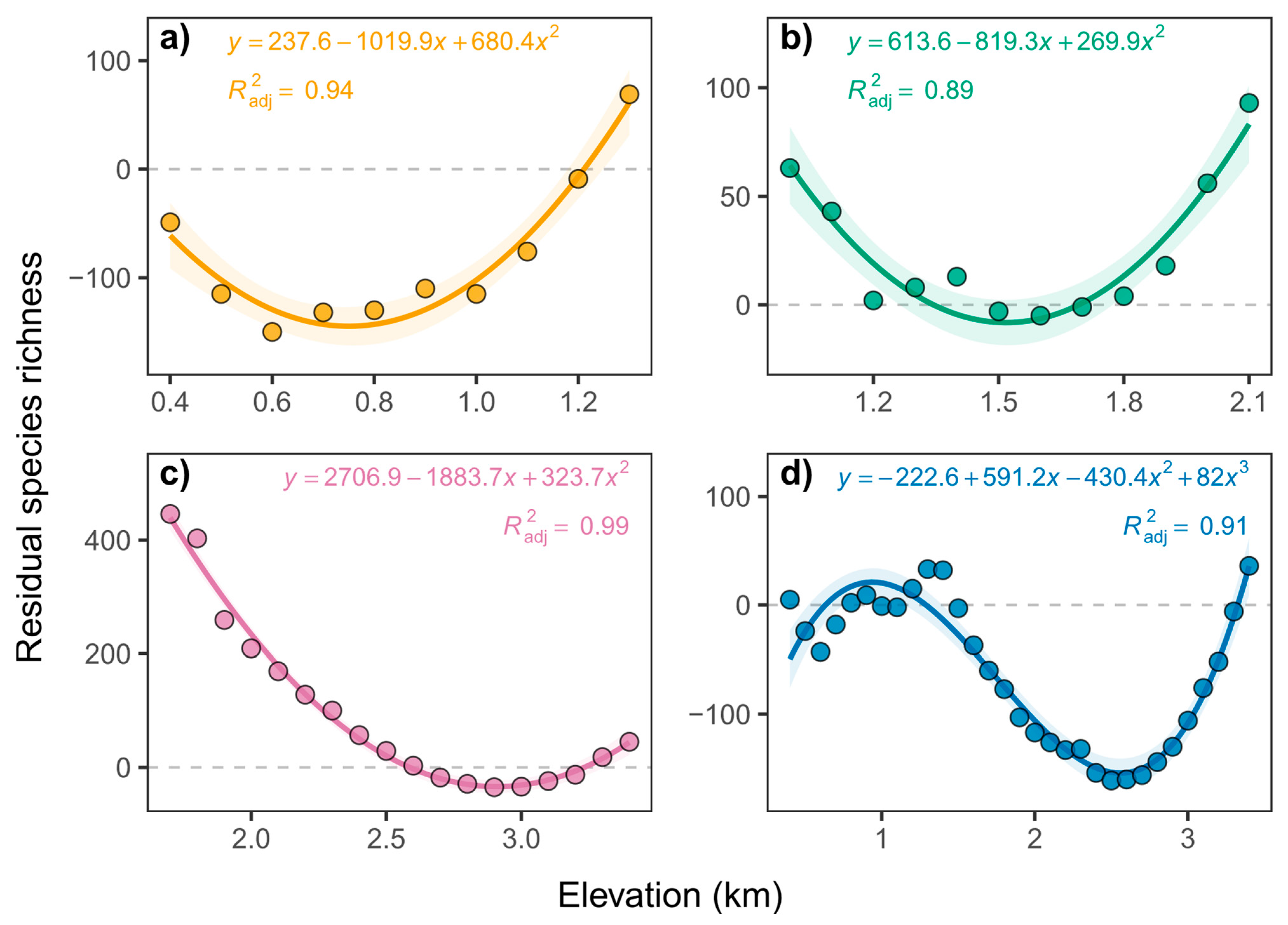
The residual species richness (the difference in the observed and predicted null richness) varied from 1 to 446 across all the selected sites. These differences ranged from 8 to 150 for the Morni Hills, 1 to 93 for the Chail WLS, 3 to 446 for the Churdhar WLS, and 1 to 161 for All Sites combined. The elevational pattern of the residual species richness followed a cubic relationship for All Sites and a quadratic relationship for the Morni Hills, Chail WLS, and Churdhar WLS (Table S4). The residual species richness tended to minimise towards lower elevations for All Sites, intermediate elevations for the Chail WLS, and higher elevations for the Morni Hills and Churdhar WLS. The residual species richness showed an increasing pattern for the Morni Hills and decreasing pattern for the Churdhar WLS with a rise in elevation. Overall, this quadratic linear model explained about 94%, 89%, and 99% of the variation in the residual species richness for the Morni Hills, Chail WLS, and Churdhar WLS, respectively (Figure 7). However, the residual species richness exhibited a strong cubic relationship with elevation for the pooled data from All Sites (Figure 7d). This cubic relationship indicated a slight increase in the residual species richness at lower elevations, then a substantial decrease at intermediate elevations and an increase at higher elevations. This cubic pattern of residual species richness suggests that the observed species richness substantially deviates from the predicted null richness at intermediate to higher elevations.

3.5. Influence of Observed Species

The elevational patterns of plant species substantially varied with the total number of observed plant species (Figure 8). The relationship between the species richness and elevation becomes steeper with the increasing number of total species across all sites. As the total number of species decreases, the richness patterns become flatter and species richness spreads across the elevational gradient. In general, the richness patterns tend to follow a unimodal distribution at higher numbers of total observed plant species for each site. For each site, the near mid-elevational richness peak (elevation with maximum species richness) showed higher sensitivity to the total number of observed species than the species richness at the lower or upper elevation limit of each study site (Figure 8). Further, the total number of observed species (N_obs) also seemed to affect the relationship between the observed richness (S) and predicted richness (S_null) by the mid-domain effect null model (Figure S7).

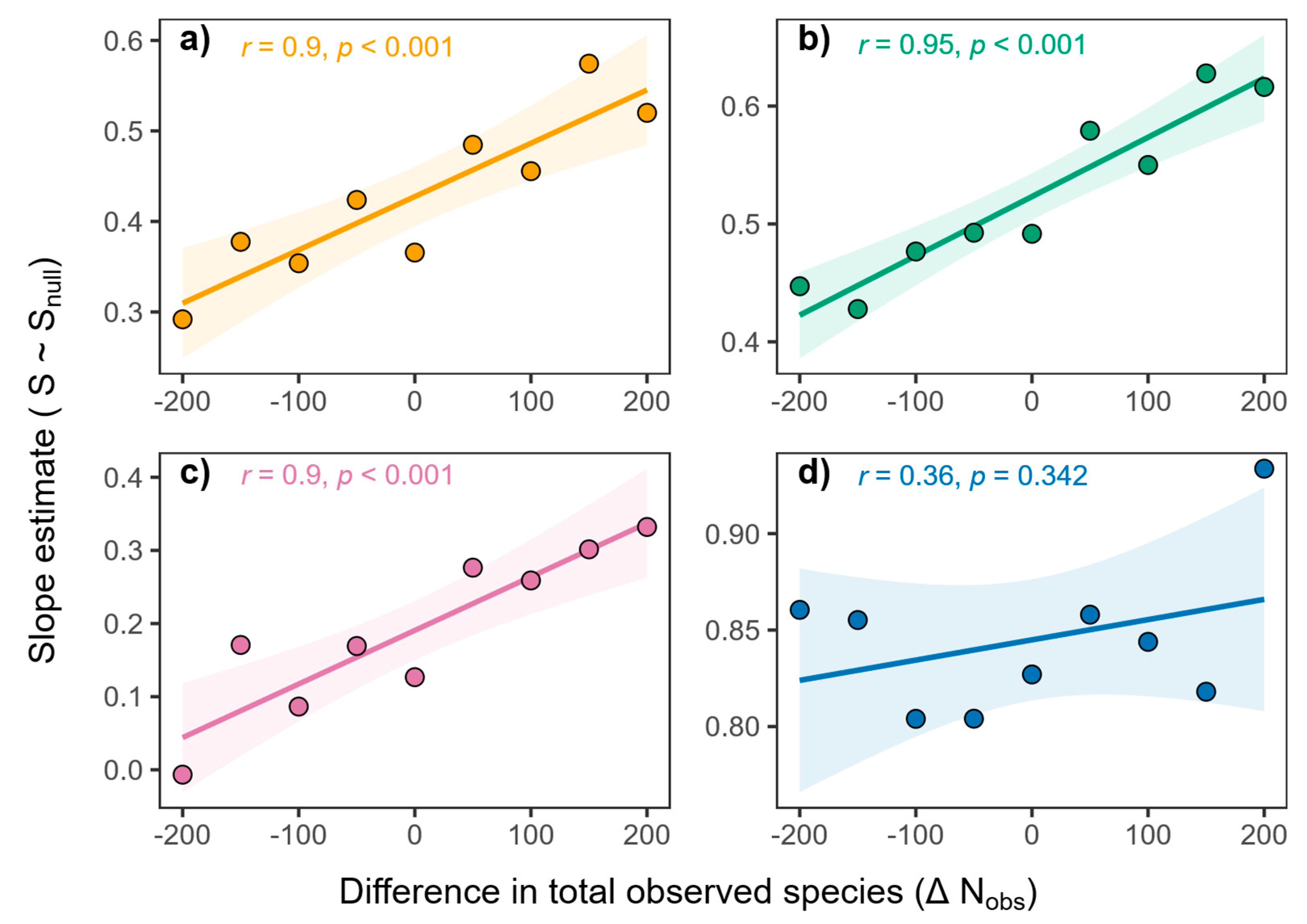
With the increase in the total number of species, the observed species richness tended to converge towards the predictions of the null model. The total number of species showed a significant positive association with the slope values estimated from the linear regression of the observed species richness against the predictions of the null model (Figure 9). These slope values showed a significant positive increase with the increase in the total number of plant species for the selected sites. The highest association was observed at intermediate elevations for the Chail WLS (r = 0.95, p < 0.001). However, the entire elevational gradient showed a non-significant positive Pearson’s correlation coefficient (r = 0.36, p = 0.342). Thus, the elevational patterns for the entire elevational gradient (All Sites) remained unaffected by the total number of plant species (Figure 9). Despite the convergence of the elevational patterns towards the predictions of the null model at a greater number of total species, the observed elevational pattern remained substantially different from the predictions of the null model (Figure S7).

4. Discussion

In this study, we aimed to explore the elevational patterns of plant species richness. Additionally, we sought to compare the observed pattern with the null predictions and examine the elevational patterns of residual plant species (i.e., the difference between observed and predicted values from the null model) to assess the influence of random processes on species richness. Our results indicated substantial variation in the observed plant taxa across sites along the elevational gradient (Question 1). Plant species richness generally exhibited a unimodal relationship with elevation, but a decreasing pattern was also observed (Question 2). Further, the observed species richness considerably deviated from the predictions of the null model across the sites (Question 3). The magnitude and direction of these deviations (residual species richness) varied along the elevation gradient. Furthermore, the residual species richness demonstrated non-linear relationships with the elevation (Question 4). Our findings provide valuable insights into the relationship between elevational gradients and plant species richness. Although the richness patterns for individual sites varied with the total number of observed species, our results for the entire elevational gradient (All Sites) showed little variation due to the total number of observed species (Figure 9). Thus, our findings for the entire elevational gradient are robust to the variation in the total number of observed species.

Our data indicated substantial differences in observed plant taxa across the three sites along the elevational gradient. We recorded a greater number of total and unique plant taxa at lower (Morni Hills) and upper (Churdhar WLS) elevations as compared to intermediate elevations (Chail WLS). Contrary to our expectations, we recorded a minimum number of total and unique plant taxa at intermediate elevations (Chail WLS). The lower records of taxa at intermediate elevations suggest the dominance of fewer plant taxa. Alternatively, this region may be under-explored and more plant taxa can be recorded in future surveys. This observation was further supported by the significantly lower species richness for the Chail WLS (intermediate elevations) than the Morni Hills (lower elevations) and Churdhar WLS (upper elevations) at standardised sampling units. Thus, our data suggests substantial variation in plant taxa across the elevational gradient in the Western Himalayas.

The primary aim of this study was to investigate the elevational patterns of plant species in the Western Himalayas, focusing on three distinct sites along an elevational gradient. The results obtained from this study revealed interesting patterns, with sites at lower (Morni Hills) and intermediate (Chail WLS) elevations displaying a unimodal distribution of plant species along the elevational gradient. In contrast, the third site (Churdhar WLS) at higher elevations exhibited a decreasing pattern. Furthermore, the entire elevational gradient (All Sites) also demonstrated a unimodal relationship between elevation and plant species richness. The unimodal pattern showed that the species richness initially increases to reach a maximum richness (mid-elevational peak) and then decreases along the elevational gradient [3,10]. This observed elevational pattern is consistent with previous research conducted in the Himalayas [28,38,40,79] and other mountain ecosystems [3,10]. In the case of plants, this pattern has been observed for bryophytes [13], pteridophytes [15,16], angiosperms [11,95], orchids [25], woody plants [28,40], and vascular plants [22,23,39,96]. Since three out of four studied elevational gradients observed this pattern, our analysis also supports the widespread unimodal relationship between elevation and species richness among plants [3,4,10].

One notable finding of the present study was the decreasing pattern of plant species richness at higher elevational gradients (Churdhar WLS). This finding aligns with earlier studies conducted in the Himalayas [19,27] and other mountain ecosystems [16,21,30]. Such a decreasing elevational pattern of species richness has also been observed for microbes [11], bryophytes [14], ferns [16], trees [19,24], and vascular plants [21,26,27]. These observations suggest that decreasing patterns of plant species richness are not uncommon, though the unimodal pattern is frequently observed [3,10]. Thus, plant species richness may not always exhibit a unimodal relationship with elevation and further studies along elevational gradients would be valuable for understanding the elevational patterns of species richness.

Another aim of the present study was to compare the observed species richness patterns to the null predictions using the mid-domain effect (MDE) null model [34]. Our results showed significant to substantial deviations in the observed species richness from the predictions of the MDE null model. Specifically, the species richness patterns at upper (Churdhar WLS) and lower (Morni Hills) elevational gradients significantly deviated from the predictions of the MDE model. This significant deviation might be due to small-ranged species because smaller ranges experience fewer geometric constraints than larger ranges [36]. Further, the observed species richness across the entire elevational gradient (All Sites) was closely matched with the predictions of the MDE model followed by the intermediate elevational gradient (Chail WLS). These close agreements with the predictions of the MDE model might be due to increased geometric constraints on species ranges. Large-ranged species at intermediate elevations and the extended scale for the entire elevational gradient might have contributed to the increased geometric constraints on species ranges. Despite variable agreement [35], we observed considerable deviations in the observed species richness from the predictions of the null model. Thus, our findings indicate that other factors beyond the range constraints may play a crucial role in shaping the elevational patterns of species richness.

In addition to comparing the observed patterns with the null predictions, we aimed to investigate the elevational pattern of residual species richness (the difference between observed species richness and predictions of the null model). The residual species richness represents the magnitude and direction of deviations from the predictions of the mid-domain effect (MDE) null model. We observed positive residual species richness for sites representing intermediate (Chail WLS) and upper (Churdhar WLS) elevational gradients. This positive deviation indicated higher observed species richness than the predictions under the null model of range constraints. On the other hand, we observed a general negative residual species richness for the entire elevational gradient (All Sites) and the site representing a lower elevation gradient (Morni Hills). This negative residual species richness suggested lower-than-expected species richness based on the range constraints alone. These deviations in the variable magnitude and directions indicate the presence of other factors driving species richness rather than the range constraints alone.

An important finding of the present study is that residual species richness showed significant quadratic relationships with elevation for the three individual sites and a significant cubic relationship for the entire elevational gradient. The significant quadratic relationships observed at the three individual sites suggest a complex pattern of species richness at smaller elevational gradients. This quadratic relationship indicates that the magnitude of deviation initially decreases with elevation, reaches a minimum, and then increases at higher elevations. Such a relationship between the elevation and magnitude of deviations indicates that the species richness patterns are shaped by the joint effects of different ecological processes along the elevational gradient. Further, the significant cubic relationship observed for the entire elevational gradient suggests a more complex and non-linear response of species richness to elevation. This cubic relationship indicates that the magnitude of deviation initially increases with elevation, reaches a peak, declines, and then potentially increases again at higher elevations. Such a pattern suggests the presence of additional factors or processes that influence species richness dynamics along the entire gradient. These factors could include large-scale climatic variables, historical and evolutionary processes, or interactions with other ecological variables that are not accounted for by the null model [32,33].

Our study revealed the influence of the total number of observed species on the elevational patterns of species richness. We showed that the richness patterns inferred from range interpolation are sensitive to the total number of observed plant species. The observed elevational patterns tend to follow a unimodal distribution with the increase in the total number of observed species. This convergence to unimodal distribution may be parallelly driven by the central limit theorem [97]. Further, our study indicated that the richness patterns varied with the total number of observed species for individual sites (N_obs < 600), but not for the entire elevational gradient (N_obs > 1000). This observation suggests that the effect of the total number of observed species is stronger at smaller scales of elevational gradients. Thus, our study indicated that a total number of species greater than 1000 and an elevational gradient of greater than 3000 metres might be useful to study the elevational patterns of species richness at larger spatial scales.

Apart from the richness patterns, the total number of observed species also influenced the relationship between the observed species richness and the predictions of the mid-domain effect null model. This relationship becomes progressively stronger with the increase in the total number of observed species. Thus, the observed richness patterns tend to fit the mid-domain effect null model with a larger number of total observed species. This convergence towards the null model may be driven by the increased proportion of large-ranged species, experiencing greater geometric constraints [34,36]. However, we showed that the effect of the total number of observed species was strongest at the intermediate elevational gradient (Chail WLS), but disappeared for the entire elevational gradient (All Sites). Thus, the magnitude of this effect seemed to also depend on the position and extent of the elevational gradient. While the effect of spatial scale (elevational extent) has been previously noted [36], our study also indicated variation due to the position of the elevational gradient. With the increase in the total number of observed species, the richness patterns tend to fit the mid-domain effect null model more rapidly at the intermediate elevational gradient than the lower or upper elevational gradient. Thus, our study highlights a complex interplay between the sample size, spatial scale, and elevational patterns of species richness.

The observed species richness showed significant deviations from the predictions of the null model and the residual species richness also demonstrated a significant quadratic or cubic relationship with elevation. These observations indicate that the observed species richness pattern cannot be achieved solely due to random processes. Our study highlights the limitations of the null model in fully capturing the observed elevational patterns of species richness. While null models provide a useful baseline for comparison and understanding broad-scale patterns, their assumptions and simplifications may not fully represent the complexity of ecological processes and interactions that shape elevational gradients. The observed deviations from the null model emphasise the need for considering additional environmental variables, biotic interactions, and historical factors when studying the elevational patterns of species richness [20,33].

Our findings have important practical implications for biodiversity conservation and management in the Western Himalayas. Firstly, the identification of mid-elevation richness peaks provides a scientific basis for prioritising conservation zones within protected areas. These habitats support the greatest diversity and should be prioritised for management and resource allocation. Secondly, the comprehensive species dataset generated in this study offers a valuable resource for long-term biodiversity monitoring, ecological restoration initiatives, and predictive species distribution modelling under future climate scenarios. Finally, by filling a regional knowledge gap in the Western Himalayas, our study contributes directly to supporting the formulation of biodiversity action plans and climate adaptation strategies in Himalayan biodiversity hotspots.

Despite the ecological significance of this study, it is important to note that the observed elevational patterns in this study are specific to the selected sites and the study area. The present study used the range interpolation method to study the elevational patterns. Although it is widely used for biogeographical and macroecological studies [22,31,37,38], it has been criticised for its assumptions of a continuous distribution of species [35,36]. Further, the data used in this study was derived from the published floral records that may contain inherent limitations. Biases may arise from incomplete species inventories and inaccurate estimations of distribution ranges, which could potentially distort the observed patterns of species richness. Nevertheless, such floristic datasets remain valuable for investigating large-scale ecological and biogeographical patterns [18,22,30]. Overall, our study highlights the importance of considering the specific characteristics and dynamics of each site when studying elevational patterns. Further, the present study underscores the importance of considering the entire elevational gradient to capture the full range of ecological dynamics and complexities involved in shaping the elevational patterns of species richness. Future studies should consider expanding the study area and incorporating additional environmental variables to gain a more comprehensive understanding of the drivers and mechanisms underlying the elevational patterns of plant species. Ecological factors, geographical context, and historical factors can significantly influence elevational patterns, and caution should be exercised when generalising these findings to other regions or ecosystems.

5. Conclusions

In conclusion, the findings of this study contribute to our understanding of biodiversity patterns along elevational gradients and have implications for biodiversity conservation and ecosystem management. The differences in the relationship between elevation and species richness across the elevational gradients emphasise the complexity of elevational patterns. Further, the deviation from the predictions of the null model highlights the importance of factors beyond range constraints (mid-domain effect) in shaping the elevational patterns of species richness. Furthermore, the quadratic or cubic relationship between elevation and residual species richness suggested the non-random distribution of plants influenced by multiple ecological processes. Climatic gradients, biotic interactions, evolutionary histories, and topographic heterogeneity can potentially contribute to generate richness patterns. Understanding these determinants is particularly important in the context of accelerating environmental change. Future research should unravel these determinants and specific mechanisms contributing to the observed richness patterns. Such studies will enhance our understanding of the ecological processes shaping biodiversity and assist in developing effective conservation strategies in the face of environmental changes.

References

1. Bánki, O.; Roskov, Y.; Döring, M.; Ower, G.; Vandepitte, L.; Hobern, D.; Remsen, D.; Schalk, P.; DeWalt, R.E.; Keping, M.; et al. Catalogue of Life Checklist (Annual Checklist 2023); Catalogue of Life: Leiden, The Netherlands, 2023. [Google Scholar] [CrossRef]
2. Rahbek, C.; Borregaard, M.K.; Colwell, R.K.; Dalsgaard, B.; Holt, B.G.; Morueta-Holme, N.; Nogues-Bravo, D.; Whittaker, R.J.; Fjeldså, J. Humboldt’s Enigma: What Causes Global Patterns of Mountain Biodiversity? Science 2019, 365, 1108–1113. [Google Scholar] [CrossRef] [PubMed]
3. Guo, Q.; Kelt, D.A.; Sun, Z.; Liu, H.; Hu, L.; Ren, H.; Wen, J. Global Variation in Elevational Diversity Patterns. Sci. Rep. 2013, 3, 3007. [Google Scholar] [CrossRef] [PubMed]
4. Rahbek, C. The Elevational Gradient of Species Richness: A Uniform Pattern? Ecography 1995, 18, 200–205. [Google Scholar] [CrossRef]
5. Lomolino, M.V. Elevation Gradients of Species-Density: Historical and Prospective Views. Glob. Ecol. Biogeogr. 2001, 10, 3–13. [Google Scholar] [CrossRef]
6. Steinbauer, M.J.; Grytnes, J.-A.; Jurasinski, G.; Kulonen, A.; Lenoir, J.; Pauli, H.; Rixen, C.; Winkler, M.; Bardy-Durchhalter, M.; Barni, E.; et al. Accelerated Increase in Plant Species Richness on Mountain Summits is Linked to Warming. Nature 2018, 556, 231–234. [Google Scholar] [CrossRef]
7. Von Humboldt, A.; Bonpland, A. Essai sur la Géographie des Plantes; Chez Levrault, Schoell et Compagnie: Paris, France, 1805; p. 274. [Google Scholar] [CrossRef]
8. Stevens, G.C. The Elevational Gradient in Altitudinal Range: An Extension of Rapoport’s Latitudinal Rule to Altitude. Am. Nat. 1992, 140, 893–911. [Google Scholar] [CrossRef] [PubMed]
9. Rahbek, C. The Role of Spatial Scale and the Perception of Large-Scale Species-Richness Patterns. Ecol. Lett. 2005, 8, 224–239. [Google Scholar] [CrossRef]
10. McCain, C.M.; Grytnes, J.A. Elevational Gradients in Species Richness. In Encyclopedia of Life Sciences (eLS); Wiley: Chichester, UK, 2010. [Google Scholar] [CrossRef]
11. Bryant, J.A.; Lamanna, C.; Morlon, H.; Kerkhoff, A.J.; Enquist, B.J.; Green, J.L. Microbes on Mountainsides: Contrasting Elevational Patterns of Bacterial and Plant Diversity. Proc. Natl. Acad. Sci. USA 2008, 105, 11505–11511. [Google Scholar] [CrossRef]
12. McCain, C.M. Global Analysis of Bird Elevational Diversity. Glob. Ecol. Biogeogr. 2009, 18, 346–360. [Google Scholar] [CrossRef]
13. Grau, O.; Grytnes, J.A.; Birks, H.J.B. A Comparison of Altitudinal Species Richness Patterns of Bryophytes with Other Plant Groups in Nepal, Central Himalaya. J. Biogeogr. 2007, 34, 1907–1915. [Google Scholar] [CrossRef]
14. Rodríguez-Quiel, E.E.; Kluge, J.; Mendieta-Leiva, G.; Bader, M.Y. Elevational Patterns in Tropical Bryophyte Diversity Differ Among Substrates: A Case Study on Baru Volcano, Panama. J. Veg. Sci. 2022, 33, e13136. [Google Scholar] [CrossRef]
15. Bhattarai, K.R.; Vetaas, O.R.; Grytnes, J.A. Fern Species Richness Along a Central Himalayan Elevational Gradient, Nepal. J. Biogeogr. 2004, 31, 389–400. [Google Scholar] [CrossRef]
16. Kessler, M.; Kluge, J.; Hemp, A.; Ohlemüller, R. A Global Comparative Analysis of Elevational Species Richness Patterns of Ferns. Glob. Ecol. Biogeogr. 2011, 20, 868–880. [Google Scholar] [CrossRef]
17. Khine, P.K.; Fraser-Jenkins, C.; Lindsay, S.; Middleton, D.; Miehe, G.; Thomas, P.; Kluge, J. A Contribution Toward the Knowledge of Ferns and Lycophytes from Northern and Northwestern Myanmar. Am. Fern J. 2017, 107, 219–256. [Google Scholar] [CrossRef]
18. Qian, H.; Kessler, M.; Vetaas, O.R. Pteridophyte Species Richness in the Central Himalaya Is Limited by Cold Climate Extremes at High Elevations and Rainfall Seasonality at Low Elevations. Ecol. Evol. 2022, 12, e8958. [Google Scholar] [CrossRef]
19. Nowak, P.; Khine, P.K.; Homeier, J.; Leuschner, C.; Miehe, G.; Kluge, J. A Plot-Based Elevational Assessment of Species Densities, Life Forms and Leaf Traits of Seed Plants in the South-Eastern Himalayan Biodiversity Hotspot, North Myanmar. Plant Ecol. Divers. 2020, 13, 437–450. [Google Scholar] [CrossRef]
20. Kumar, A. Climate-Driven Elevational Shifting of Plant Distributions in the Selected Sites of Siwaliks of North Western India. Ph.D. Thesis, Panjab University, Chandigarh, India, 2024; p. 259. Available online: http://hdl.handle.net/10603/607391 (accessed on 26 September 2025).
21. Trigas, P.; Panitsa, M.; Tsiftsis, S. Elevational Gradient of Vascular Plant Species Richness and Endemism in Crete—The Effect of Post-Isolation Mountain Uplift on a Continental Island System. PLoS ONE 2013, 8, e59425. [Google Scholar] [CrossRef]
22. Vetaas, O.R.; Grytnes, J.A. Distribution of Vascular Plant Species Richness and Endemic Richness Along the Himalayan Elevation Gradient in Nepal. Glob. Ecol. Biogeogr. 2002, 11, 291–301. [Google Scholar] [CrossRef]
23. Acharya, B.K.; Chettri, B.; Vijayan, L. Distribution Pattern of Trees Along an Elevation Gradient of Eastern Himalaya, India. Acta Oecol. 2011, 37, 329–336. [Google Scholar] [CrossRef]
24. Homeier, J.; Breckle, S.-W.; Günter, S.; Rollenbeck, R.T.; Leuschner, C. Tree Diversity, Forest Structure and Productivity Along Altitudinal and Topographical Gradients in a Species-Rich Ecuadorian Montane Rain Forest. Biotropica 2010, 42, 140–148. [Google Scholar] [CrossRef]
25. Djordjević, V.; Tsiftsis, S.; Kindlmann, P.; Stevanović, V. Orchid Diversity Along an Altitudinal Gradient in the Central Balkans. Front. Ecol. Evol. 2022, 10, 929266. [Google Scholar] [CrossRef]
26. Peters, M.K.; Hemp, A.; Appelhans, T.; Behler, C.; Classen, A.; Detsch, F.; Ensslin, A.; Ferger, S.W.; Frederiksen, S.B.; Gebert, F.; et al. Predictors of Elevational Biodiversity Gradients Change from Single Taxa to the Multi-Taxa Community Level. Nat. Commun. 2016, 7, 13736. [Google Scholar] [CrossRef]
27. Bisht, M.; Sekar, K.C.; Mukherjee, S.; Thapliyal, N.; Bahukhandi, A.; Singh, D.; Bhojak, P.; Mehta, P.; Upadhyay, S.; Dey, D. Influence of Anthropogenic Pressure on the Plant Species Richness and Diversity Along the Elevation Gradients of Indian Himalayan High-Altitude Protected Areas. Front. Ecol. Evol. 2022, 10, 751989. [Google Scholar] [CrossRef]
28. Khuroo, A.A.; Weber, E.; Malik, A.H.; Reshi, Z.A.; Dar, G.H. Altitudinal Distribution Patterns of the Native and Alien Woody Flora in Kashmir Himalaya, India. Environ. Res. 2011, 111, 967–977. [Google Scholar] [CrossRef]
29. Li, L.; Xu, X.; Qian, H.; Huang, X.; Liu, P.; Landis, J.B.; Fu, Q.; Sun, L.; Wang, H.; Sun, H.; et al. Elevational Patterns of Phylogenetic Structure of Angiosperms in a Biodiversity Hotspot in Eastern Himalaya. Divers. Distrib. 2022, 28, 2534–2548. [Google Scholar] [CrossRef]
30. Di Musciano, M.; Zannini, P.; Ferrara, C.; Spina, L.; Nascimbene, J.; Vetaas, O.R.; Bhatta, K.P.; D’Agostino, M.; Peruzzi, L.; Carta, A.; et al. Investigating Elevational Gradients of Species Richness in a Mediterranean Plant Hotspot Using a Published Flora. Front. Biogeogr. 2021, 13, e50007. [Google Scholar] [CrossRef]
31. Grytnes, J.A.; Vetaas, O.R. Species Richness and Altitude: A Comparison Between Null Models and Interpolated Plant Species Richness Along the Himalayan Altitudinal Gradient, Nepal. Am. Nat. 2002, 159, 294–304. [Google Scholar] [CrossRef]
32. Gaston, K.J. Global Patterns in Biodiversity. Nature 2000, 405, 220–227. [Google Scholar] [CrossRef] [PubMed]
33. Kumar, A.; Patil, M.; Kumar, P.; Singh, A.N. Determinants of Plant Species Richness Along Elevational Gradients: Insights with Climate, Energy and Water–Energy Dynamics. Ecol. Process. 2024, 13, 86. [Google Scholar] [CrossRef]
34. Colwell, R.K.; Lees, D.C. The Mid-Domain Effect: Geometric Constraints on the Geography of Species Richness. Trends Ecol. Evol. 2000, 15, 70–76. [Google Scholar] [CrossRef]
35. Colwell, R.K.; Rahbek, C.; Gotelli, N.J. The Mid-Domain Effect and Species Richness Patterns: What Have We Learned so Far? Am. Nat. 2004, 163, E1–E23. [Google Scholar] [CrossRef] [PubMed]
36. Dunn, R.R.; McCain, C.M.; Sanders, N.J. When Does Diversity Fit Null Model Predictions? Scale and Range Size Mediate the Mid-Domain Effect. Glob. Ecol. Biogeogr. 2007, 16, 305–312. [Google Scholar] [CrossRef]
37. Hu, W.; Wu, F.; Gao, J.; Yan, D.; Liu, L.; Yang, X. Influences of Interpolation of Species Ranges on Elevational Species Richness Gradients. Ecography 2016, 40, 1231–1241. [Google Scholar] [CrossRef]
38. Rana, S.K.; Gross, K.; Price, T.D. Drivers of Elevational Richness Peaks, Evaluated for Trees in the East Himalaya. Ecology 2019, 100, e02548. [Google Scholar] [CrossRef]
39. Chawla, A.; Rajkumar, S.; Singh, K.N.; Lal, B.; Singh, R.D.; Thukral, A.K. Plant Species Diversity Along an Altitudinal Gradient of Bhabha Valley in Western Himalaya. J. Mt. Sci. 2008, 5, 157–177. [Google Scholar] [CrossRef]
40. Oommen, M.A.; Shanker, K. Elevational Species Richness Patterns Emerge from Multiple Local Mechanisms in Himalayan Woody Plants. Ecology 2005, 86, 3039–3047. [Google Scholar] [CrossRef]
41. Beck, H.E.; Zimmermann, N.E.; McVicar, T.R.; Vergopolan, N.; Berg, A.; Wood, E.F. Present and Future Köppen-Geiger Climate Classification Maps at 1-Km Resolution. Sci. Data 2018, 5, 180214. [Google Scholar] [CrossRef]
42. Champion, H.G.; Seth, S.K. A Revised Survey of the Forest Types of India; Government of India: Delhi, India, 1968; p. 404. [Google Scholar]
43. IUCN. The IUCN Red List of Threatened Species; Version 2022-2. 2023. Available online: https://www.iucnredlist.org/ (accessed on 17 June 2023).
44. Rahmani, A.R.; Islam, M.Z.; Kasambe, R.M. Important Bird and Biodiversity Areas in India: Priority Sites for Conservation (Revised and Updated), 2nd ed.; Bombay Natural History Society and BirdLife International: Mumbai, India; Cambridge, UK, 2016; Volume 1, p. 1992. [Google Scholar]
45. Walter, H.; Lieth, H.H.F. Klimadiagramm-Weltatlas; G. Fischer: Jena, Germany, 1967. [Google Scholar]
46. Fick, S.E.; Hijmans, R.J. WorldClim 2: New 1-Km Spatial Resolution Climate Surfaces for Global Land Areas. Int. J. Climatol. 2017, 37, 4302–4315. [Google Scholar] [CrossRef]
47. eFI. eFlora of India: Database of Plants of Indian Subcontinent. 2023. Available online: https://efloraofindia.com/ (accessed on 17 April 2023).
48. FOI. Flowers of India. 2023. Available online: http://www.flowersofindia.net/ (accessed on 17 April 2023).
49. Kumar, A.; Patil, M.; Kumar, P.; Kumar, M.; Singh, A.N. Plant Ecology in Indian Siwalik Range: A Systematic Map and Its Bibliometric Analysis. Trop. Ecol. 2022, 63, 338–350. [Google Scholar] [CrossRef]
50. Balkrishna, A.; Srivastava, A.; Shukla, B.; Mishra, R.; Joshi, B. Medicinal Plants of Morni Hills, Shivalik Range, Panchkula, Haryana. J. Non-Timber For. Prod. 2018, 25, 1–14. [Google Scholar] [CrossRef]
51. Balkrishna, A.; Joshi, B.; Srivastava, A.; Shukla, B. Phyto-Resources of Morni Hills, Panchkula, Haryana. J. Non-Timber For. Prod. 2018, 25, 91–98. [Google Scholar] [CrossRef]
52. Dhiman, H.; Saharan, H.; Jakhar, S. Floristic Diversity Assessment and Vegetation Analysis of the Upper Altitudinal Ranges of Morni Hills, Panchkula, Haryana, India. Asian J. Conserv. Biol. 2020, 9, 134–142. [Google Scholar]
53. Dhiman, H.; Saharan, H.; Jakhar, S. Study of Invasive Plants in Tropical Dry Deciduous Forests—Biological Spectrum, Phenology, and Diversity. For. Stud. 2021, 74, 58–71. [Google Scholar] [CrossRef]
54. Singh, N.; Vashistha, B.D. Flowering Plant Diversity and Ethnobotany of Morni Hills, Siwalik Range, Haryana, India. Int. J. Pharma Bio Sci. 2014, 5, B214–B222. [Google Scholar]
55. Bhardwaj, A.; Verma, R.K.; Rana, J.C.; Thakur, K.; Verma, J. Orchid diversity at Chail Wild life Sanctuary, Himachal Pradesh, Northwest Himalaya. J. Orchid Soc. India 2014, 28, 67–74. [Google Scholar]
56. Bhardwaj, A. Study on Dynamics of Plant Bioresources in Chail Wildlife Sanctuary of Himachal Pradesh. Ph.D. Thesis, Forest Research Institute (Deemed) University, Dehradun, India, 2017; p. 342. Available online: http://hdl.handle.net/10603/175719 (accessed on 5 October 2019).
57. Kumar, R. Studies on Plant Biodiversity of Chail Wildlife Sanctuary in Himachal Pradesh. Master’s Thesis, Dr Yashwant Singh Parmar University of Horticulture and Forestry, Solan, India, 2013; p. 119. Available online: http://krishikosh.egranth.ac.in/handle/1/91126 (accessed on 4 October 2019).
58. Choudhary, A.K.; Punam; Sharma, P.K.; Chandel, S. Study on the Physiography and Biodiversity of Churdhar Wildlife Sanctuary of Himachal Himalayas, India. Tigerpaper 2007, 34, 27–32. [Google Scholar]
59. Choudhary, R.K.; Lee, J. A Floristic Reconnaissance of Churdhar Wildlife Sanctuary of Himachal Pradesh, India. Manthan 2012, 13, 2–12. [Google Scholar]
60. Gupta, H. Comparative Studies on the Medicinal and Aromatic Flora of Churdhar and Rohtang Areas of Himachal Pradesh. Master’s Thesis, Dr Yashwant Singh Parmar University of Horticulture and Forestry, Solan, India, 1998; p. 228. Available online: http://krishikosh.egranth.ac.in/handle/1/5810135063 (accessed on 11 August 2022).
61. Radha; Puri, S.; Chandel, K.; Pundir, A.; Thakur, M.S.; Chauhan, B.; Simer, K.; Dhiman, N.; Shivani; Thakur, Y.S.; et al. Diversity of Ethnomedicinal Plants in Churdhar Wildlife Sanctuary of District Sirmour of Himachal Pradesh, India. J. Appl. Pharm. Sci. 2019, 9, 48–53. [Google Scholar] [CrossRef]
62. Subramani, S.P.; Kapoor, K.S.; Goraya, G.S. Additions to the Floral Wealth of Sirmaur District, Himachal Pradesh from Churdhar Wildlife Sanctuary. J. Threat. Taxa 2014, 6, 6427–6452. [Google Scholar] [CrossRef]
63. Thakur, U.; Bisht, N.S.; Kumar, M.; Kumar, A. Influence of Altitude on Diversity and Distribution Pattern of Trees in Himalayan Temperate Forests of Churdhar Wildlife Sanctuary, India. Water Air Soil Pollut. 2021, 232, 205. [Google Scholar] [CrossRef]
64. Govaerts, R.; Lughadha, E.N.; Black, N.; Turner, R.; Paton, A. The World Checklist of Vascular Plants, a Continuously Updated Resource for Exploring Global Plant Diversity. Sci. Data 2021, 8, 215. [Google Scholar] [CrossRef]
65. Turland, N.; Wiersema, J.; Barrie, F.; Greuter, W.; Hawksworth, D.; Herendeen, P.; Knapp, S.; Kusber, W.-H.; Li, D.-Z.; Marhold, K.; et al. (Eds.) International Code of Nomenclature for Algae, Fungi, and Plants (Shenzhen Code); Regnum vegetabile; Koeltz Botanical Books: Glashütten, Germany, 2018; Volume 159, p. 254. ISBN 978-3-946583-16-5. [Google Scholar] [CrossRef]
66. APG, I.V. An Update of the Angiosperm Phylogeny Group Classification for the Orders and Families of Flowering Plants: APG IV. Bot. J. Linn. Soc. 2016, 181, 1–20. [Google Scholar] [CrossRef]
67. POWO. Plants of the World Online; Royal Botanic Gardens: Kew, UK, 2022; Available online: http://www.plantsoftheworldonline.org/ (accessed on 8 August 2022).
68. Brown, M.J.M.; Walker, B.E.; Black, N.; Govaerts, R.H.A.; Ondo, I.; Turner, R.; Lughadha, E.N. rWCVP: A Companion R Package for the World Checklist of Vascular Plants. New Phytol. 2023, 240, 1355–1365. [Google Scholar] [CrossRef]
69. Rana, S.K.; Rawat, G.S. Database of Himalayan Plants Based on Published Floras During a Century. Data 2017, 2, 36. [Google Scholar] [CrossRef]
70. Rana, S.K.; Rawat, G.S. Database of Vascular Plants of Himalaya, version 1.6; Wildlife Institute of India: Dehradun, India, 2019. [Google Scholar] [CrossRef]
71. Chowdhery, H.J.; Wadhwa, B.M. Flora of Himachal Pradesh; Botanical Survey of India: Calcutta, India, 1984; Volumes 1–3. [Google Scholar]
72. Collett, H. Flora Simlensis; Thacker, Spink & Co.: Simla, India, 1902. [Google Scholar] [CrossRef]
73. Duthie, J.F. Flora of the Upper Gangetic Plain, and of the Adjacent Siwalik and Sub-Himalayan Tracts; Superintendent of Government Printing: Calcutta, India, 1903–1915; Volumes 1–3. [Google Scholar] [CrossRef]
74. Chamberlain, S.; Barve, V.; Mcglinn, D.; Oldoni, D.; Desmet, P.; Geffert, L.; Ram, K. rgbif: Interface to the Global Biodiversity Information Facility API. CRAN. 2025. Available online: https://cran.r-project.org/web/packages/rgbif/index.html (accessed on 13 October 2025).
75. Rana, S.K.; Price, T.D.; Qian, H. Plant Species Richness Across the Himalaya Driven by Evolutionary History and Current Climate. Ecosphere 2019, 10, e02945. [Google Scholar] [CrossRef]
76. Colwell, R.K.; Hurtt, G.C. Nonbiological Gradients in Species Richness and a Spurious Rapoport Effect. Am. Nat. 1994, 144, 570–595. [Google Scholar] [CrossRef]
77. Hollister, J.; Shah, T.; Robitaille, A.L.; Beck, M.W.; Johnson, M. elevatr: Access Elevation Data from Various APIs; Zenodo: Geneva, Switzerland, 2021. [Google Scholar] [CrossRef]
78. Hijmans, R.J. terra: Spatial Data Analysis. CRAN. 2025. Available online: https://cran.r-project.org/web/packages/terra/index.html (accessed on 13 October 2025).
79. Manish, K.; Pandit, M.K.; Telwala, Y.; Nautiyal, D.C.; Koh, L.P.; Tiwari, S. Elevational Plant Species Richness Patterns and Their Drivers Across Non-Endemics, Endemics and Growth Forms in the Eastern Himalaya. J. Plant Res. 2017, 130, 829–844. [Google Scholar] [CrossRef]
80. Gao, C.; Chen, C.; Akyol, T.; Dusa, A.; Yu, G.; Cao, B.; Cai, P. ggVennDiagram: Intuitive Venn Diagram Software Extended. iMeta 2024, 3, e177. [Google Scholar] [CrossRef]
81. Chao, A.; Gotelli, N.J.; Hsieh, T.C.; Sander, E.L.; Ma, K.H.; Colwell, R.K.; Ellison, A.M. Rarefaction and Extrapolation with Hill Numbers: A Framework for Sampling and Estimation in Species Diversity Studies. Ecol. Monogr. 2014, 84, 45–67. [Google Scholar] [CrossRef]
82. Colwell, R.K.; Mao, C.X.; Chang, J. Interpolating, Extrapolating, and Comparing Incidence-based Species Accumulation Curves. Ecology 2004, 85, 2717–2727. [Google Scholar] [CrossRef]
83. Colwell, R.K.; Chao, A.; Gotelli, N.J.; Lin, S.-Y.; Mao, C.X.; Chazdon, R.L.; Longino, J.T. Models and Estimators Linking Individual-Based and Sample-Based Rarefaction, Extrapolation and Comparison of Assemblages. J. Plant Ecol. 2012, 5, 3–21. [Google Scholar] [CrossRef]
84. Kumar, A.; Kumar, P.; Patil, M.; Hussain, S.; Yadav, R.; Sharma, S.; Tokas, D.; Singh, S.; Singh, A.N. Disturbance and Vegetational Structure in an Urban Forest of Indian Siwaliks: An Ecological Assessment. Environ. Monit. Assess. 2024, 196, 691. [Google Scholar] [CrossRef]
85. R Core Team. R: A Language and Environment for Statistical Computing; R Foundation for Statistical Computing: Vienna, Austria, 2024; Available online: https://www.r-project.org/ (accessed on 31 October 2024).
86. Hsieh, T.C.; Ma, K.H.; Chao, A. iNEXT: An R Package for Rarefaction and Extrapolation of Species Diversity (Hill Numbers). Methods Ecol. Evol. 2016, 7, 1451–1456. [Google Scholar] [CrossRef]
87. Hilbe, J.M. Modeling Count Data; Cambridge University Press: Cambridge, UK, 2014. [Google Scholar] [CrossRef]
88. Johnson, J.B.; Omland, K.S. Model Selection in Ecology and Evolution. Trends Ecol. Evol. 2004, 19, 101–108. [Google Scholar] [CrossRef]
89. Burnham, K.P.; Anderson, D.R. (Eds.) Model Selection and Multimodel Inference, 2nd ed.; Springer: New York, NY, USA, 2002; p. 488. [Google Scholar] [CrossRef]
90. Hurvich, C.M.; Tsai, C.-L. Regression and Time Series Model Selection in Small Samples. Biometrika 1989, 76, 297–307. [Google Scholar] [CrossRef]
91. Dunn, P.K.; Smyth, G.K. Randomized Quantile Residuals. J. Comput. Graph. Stat. 1996, 5, 236–244. [Google Scholar] [CrossRef]
92. Hartig, F. DHARMa: Residual Diagnostics for Hierarchical (Multi-Level/Mixed) Regression Models. CRAN. 2024. Available online: https://cran.r-project.org/web/packages/DHARMa/index.html (accessed on 13 October 2025).
93. Gotelli, N.J.; Anderson, M.J.; Arita, H.T.; Chao, A.; Colwell, R.K.; Connolly, S.R.; Currie, D.J.; Dunn, R.R.; Graves, G.R.; Green, J.L.; et al. Patterns and Causes of Species Richness: A General Simulation Model for Macroecology. Ecol. Lett. 2009, 12, 873–886. [Google Scholar] [CrossRef] [PubMed]
94. Wickham, H.; Averick, M.; Bryan, J.; Chang, W.; McGowan, L.; François, R.; Grolemund, G.; Hayes, A.; Henry, L.; Hester, J.; et al. Welcome to the Tidyverse. J. Open Source Softw. 2019, 4, 1686. [Google Scholar] [CrossRef]
95. Manish, K. Species Richness, Phylogenetic Diversity and Phylogenetic Structure Patterns of Exotic and Native Plants Along an Elevational Gradient in the Himalaya. Ecol. Process. 2021, 10, 64. [Google Scholar] [CrossRef]
96. Thorne, J.H.; Choe, H.; Dorji, L.; Yangden, K.; Wangdi, D.; Phuntsho, Y.; Beardsley, K. Species Richness and Turnover Patterns for Tropical and Temperate Plants on the Elevation Gradient of the Eastern Himalayan Mountains. Front. Ecol. Evol. 2022, 10, 942759. [Google Scholar] [CrossRef]
97. Fischer, H. A History of the Central Limit Theorem: From Classical to Modern Probability Theory; Springer: New York, NY, USA, 2011; p. 402. [Google Scholar] [CrossRef]
Figure 1. Geographic location of Morni Hills, Chail WLS, and Churdhar WLS in Western Himalayas. The Khol Hi-Raitan (KHR) WLS is located in the western part of the Morni Hills. The inset map shows the northern states of India including Ladakh (LA), Jammu and Kashmir (JK), Himachal Pradesh (HP), Punjab (PB), and Uttarakhand (UK). The study sites are located in the southern part of Himachal Pradesh (HP) and shared by the northern part of Haryana state.
Forests 16 01591 g001
Figure 3. Venn diagram illustrating the distribution of taxa (a) species (n = 1385), (b) genera (n = 748), and (c) families (n = 145) across the study sites. Each circle represents a specific site and the overlapping areas represent shared taxa, while the non-overlapping regions indicate unique taxa for each site. The numbers represent the count of taxa for each shared or unique category across the study sites.
Forests 16 01591 g003
Figure 4. Comparison of sample size-based rarefaction and extrapolation curves of species richness for the lower (Morni Hills), intermediate (Chail WLS), and upper elevational gradient (Churdhar WLS). The points represent the observed species richness, the solid lines represent the rarefied species richness, the dashed lines represent the extrapolated species richness, and the shaded lines represent the 95% confidence intervals for the estimates based on bootstrap procedures (n = 100).
Forests 16 01591 g004
Figure 5. Elevational patterns of estimated species richness (solid line) plotted against the predictions of the null model (dashed line) for (a) Morni Hills, (b) Chail WLS, (c) Churdhar WLS, and (d) All Sites. The data points (filled circles) represent the estimated species richness for each 100 m elevational band. The smooth line for estimated richness was fitted using the polynomial Poisson generalised linear model (GLM) with log-link function. The shaded region around the fitted solid line represents the 95% confidence intervals. The null model predictions represent the mean (dashed line) with minimum and maximum (grey-shaded region) predicted species richness from 10,000 random simulations.
Forests 16 01591 g005
Figure 6. Scatter plot showing the relationship between observed and predicted species richness for (a) Morni Hills, (b) Chail WLS, (c) Churdhar WLS, and (d) All Sites. The coloured solid line represents the fitted regression line and the shaded region represents the 95% confidence intervals. The estimated regression coefficients are represented as a regression equation with the adjusted coefficient of determination (R2adj). The observed species richness was used as the response variable and the predicted species richness was used as a predictor variable. The grey dashed line indicates the 1:1 line.
Forests 16 01591 g006
Figure 7. Elevational patterns of residual species richness (Sres) for (a) Morni Hills, (b) Chail WLS, (c) Churdhar WLS, and (d) All Sites. The residual species richness (Sres) is calculated as the difference between the observed species richness (S) and null species richness (Snull). The null species richness (Snull) is the mean of the predicted species richness from 10,000 replications of the mid-domain effect null model. The data points (filled circles) represent the residual species richness for each 100 m elevational band. The smooth line was fitted using the polynomial linear regression with residual species richness (Sres) as the response variable and elevation as the predictor variable. The shaded region around the fitted line represents the 95% confidence intervals. The estimated regression equation and the adjusted coefficient of determination (R2adj) for each site are also presented. The grey dashed line indicates the zero residual species richness, i.e., observed species richness is perfectly identical to predicted species richness.
Forests 16 01591 g007
Figure 8. Influence of total number of observed species (Nobs) on elevational patterns of plant species richness for (a) Morni Hills, (b) Chail WLS, (c) Churdhar WLS, and (d) All Sites. The smooth line was fitted using the polynomial Poisson generalised linear model (GLM) with log-link function (see Table 2). The shaded region around the fitted solid line represents the 95% confidence intervals. The legend shows the difference in the total number of observed species for Morni Hills (Nobs = 568), Chail WLS (Nobs = 377), Churdhar WLS (Nobs = 561), and All Sites (Nobs = 1159).
Forests 16 01591 g008
Figure 9. Effect of total number of observed species (Nobs) on the relationship between observed richness (S) and predicted richness (Snull) by mid-domain effect null model for (a) Morni Hills, (b) Chail WLS, (c) Churdhar WLS, and (d) All Sites. The slope value was estimated using a general linear model with observed species richness (S) as the response variable and the predicted species richness (Snull) as the predictor variable. The total numbers of observed species (Nobs) for Morni Hills, Chail WLS, Churdhar WLS, and All Sites were 568, 377, 561, and 1159, respectively. The solid line represents the fitted linear regression line and the shaded region represents the 95% confidence intervals. The strength and direction of association was estimated using the Pearson’s correlation coefficient (r) and associated statistical significance (p-value).
Forests 16 01591 g009