Due Diligence for Deforestation-Free Supply Chains with Copernicus Sentinel-2 Imagery and Machine Learning

Abstract

At COP26, the Glasgow Leaders Declaration committed to ending deforestation by 2030. Implementing deforestation-free supply chains is of growing importance to importers and exporters but challenging due to the complexity of supply chains for agricultural commodities which are driving tropical deforestation. Monitoring tools are needed that alert companies of forest losses around their source farms. ForestMind has developed compliance monitoring tools for deforestation-free supply chains. The system delivers reports to companies based on automated satellite image analysis of forest loss around farms. We describe an algorithm based on the Python for Earth Observation (PyEO) package to deliver near-real-time forest alerts from Sentinel-2 imagery and machine learning. A Forest Analyst interprets the multi-layer raster analyst report and creates company reports for monitoring supply chains. We conclude that the ForestMind extension of PyEO with its hybrid change detection from a random forest model and NDVI differencing produces actionable farm-scale reports in support of the EU Deforestation Regulation. The user accuracy of the random forest model was 96.5% in Guatemala and 93.5% in Brazil. The system provides operational insights into forest loss around source farms in countries from which commodities are imported.

1. Introduction

At the COP 26 Climate Conference in Glasgow in 2021, world leaders endorsed the Glasgow Leaders Declaration on Forests and Land Use, which has the goal of halting and reversing deforestation and forest degradation by 2030. Chakravarty et al. [1] identify the expansion of farmland in the tropics as the primary cause of deforestation worldwide and review its effects and control strategies. To create transparency on the deforestation impacts of supply chains, large trading blocks, including the US, EU, and UK, are in the process of introducing legislation to tackle deforestation in food supply chains that will place due diligence requirements on various supply chain actors trading in certain deforestation related commodities [2,3,4].

The European Council and the European Parliament reached a provisional political agreement on an EU Regulation on deforestation-free supply chains on 6 December 2022 [2]. On 29 June 2023, the EU Regulation on deforestation-free products (EU) 2023/1115 entered into force. It aims to ensure that certain key goods on the EU single market will no longer contribute to deforestation and forest degradation. All relevant companies have to conduct strict due diligence if they import or export any product from the following list to/from the EU single market: palm oil, cattle, soy, coffee, cocoa, timber, and rubber as well as derived products such as beef, furniture, or chocolate [2]. Any trader wishing to sell listed commodities on the EU single market or export from within it must prove that the products do not originate from recently deforested land or have contributed to forest degradation.

Due to the inaccessibility and cost of inspecting distant and often large forest areas through field visits to meet the due diligence requirements of importers and exporters, Earth observation (EO) from space is required to allow companies to demonstrate that they meet the EU Deforestation Regulation. Ideally, businesses want to receive information on any possible violation of their zero-deforestation policies in source regions for these products as soon as practicable, so they can intervene in deforestation and degradation in a timely manner. Hence, near-real-time EO data streams from operational satellite missions can provide solutions towards enabling such a due diligence system.

In addition to legislative pressures, commodity traders, retailers and brands are voluntarily making deforestation-free commitments with their products and seeking to verify these claims. Accurate, scalable solutions are required to assist companies in removing deforestation from their supply chains both to meet these commitments and to assist in corporate responsibility reporting more broadly.

A number of different solutions towards operational deforestation monitoring have been developed [5,6,7]. Strictly speaking, EO provides only information on the loss of tree cover, but not on deforestation as defined in international laws. The United Nations Framework Convention on Climate Change (UNFCCC) has a definition of deforestation that was adopted in 2001 by its Conference of the Parties (COP) 7 (11/CP.7). According to the UNFCCC (Decision 11/CP.7, 2001), deforestation is ‘the direct human-induced conversion of forested land to non-forested land’ [8]. This definition implies that the conversion of forested land to non-forested land must be human induced. It excludes natural disturbances, for example. The UN Food and Agriculture Organisation (FAO), in the same year, defined deforestation as ‘The conversion of forest to another land use or the long-term reduction of the tree canopy cover below the minimum 10 percent threshold’ [8]. The inclusion of a minimum tree canopy cover is appealing from an operational point of view, but the 10 percent tree cover threshold is not universally accepted in national forest definitions—there is in fact a huge spread of definitions [9]. The FAO definition also includes a reference to a long-term reduction in tree cover, which, strictly speaking, excludes certain types of forest cover loss from the definition of deforestation, e.g., if a primary forest is logged and then replanted by other trees. A more precise terminology for EO-derived information services is, therefore, to use forest cover loss or tree cover loss to describe the observed loss of trees, without making any assumptions about the drivers of the loss (human or natural) and about the longevity of this loss.

Forest cover loss monitoring from EO data has been demonstrated from a variety of sensors and satellite platforms. The two primary sensor types are Synthetic Aperture Radar (SAR) and multispectral imaging sensors. The main SAR applications for detecting forest cover loss include the JJFAST algorithm (‘JICA-JAXA Forest Early Warning System in the Tropics’) [10] from the Advanced Land Observation Satellite (ALOS-2) Phased Array L-band Synthetic Aperture Radar (PALSAR-2) and the RAdar for Detecting Deforestation (RADD) alerts [11,12] based on Sentinel-1, a C-band radar satellite constellation by the European Space Agency under the Copernicus Programme. Multispectral forest cover loss applications include the Global Land Analysis and Discovery (GLAD) alert system by Global Forest Watch [7] based on Hansen et al.’s [13] global tree cover change monitoring method at 30 m resolution, and the Sentinel-2-based Python for Earth Observation (PyEO) forest alert system [14], which was developed by the UK National Centre for Earth Observation at the University of Leicester together with the Kenya Forest Service and the REDD+ Stakeholder Round Table in Kenya. PyEO has been adopted by the Government of Kenya under its National Forest Monitoring Programme. The PyEO forest alert system has also been applied in other countries including Mexico and Colombia [15] and Brazil and Guatemala (this paper). Recently, some authors have suggested the adoption of combined SAR/multispectral forest cover loss monitoring systems [16,17].

While many of the published forest cover loss detection systems described above aim at large-scale or global mapping, forest monitoring solutions from space are still lacking for many parts of the world (e.g., [18]). This is especially the case for farm-scale monitoring of forest cover loss. This study in the ForestMind project aimed to answer the research question of whether an adaptation of PyEO’s forest alerts system is usable for supply chain monitoring at the farm scale. The objectives of the study were to (i) train a random forest machine learning model of forest cover, (ii) enhance the quality of the forest loss detections from post-classification change detection by combining the algorithm with differential NDVI data, (iii) produce forest loss reports in an operational scenario, and (iv) assess the accuracy of the company reports provided by the system.

2. Materials and Methods

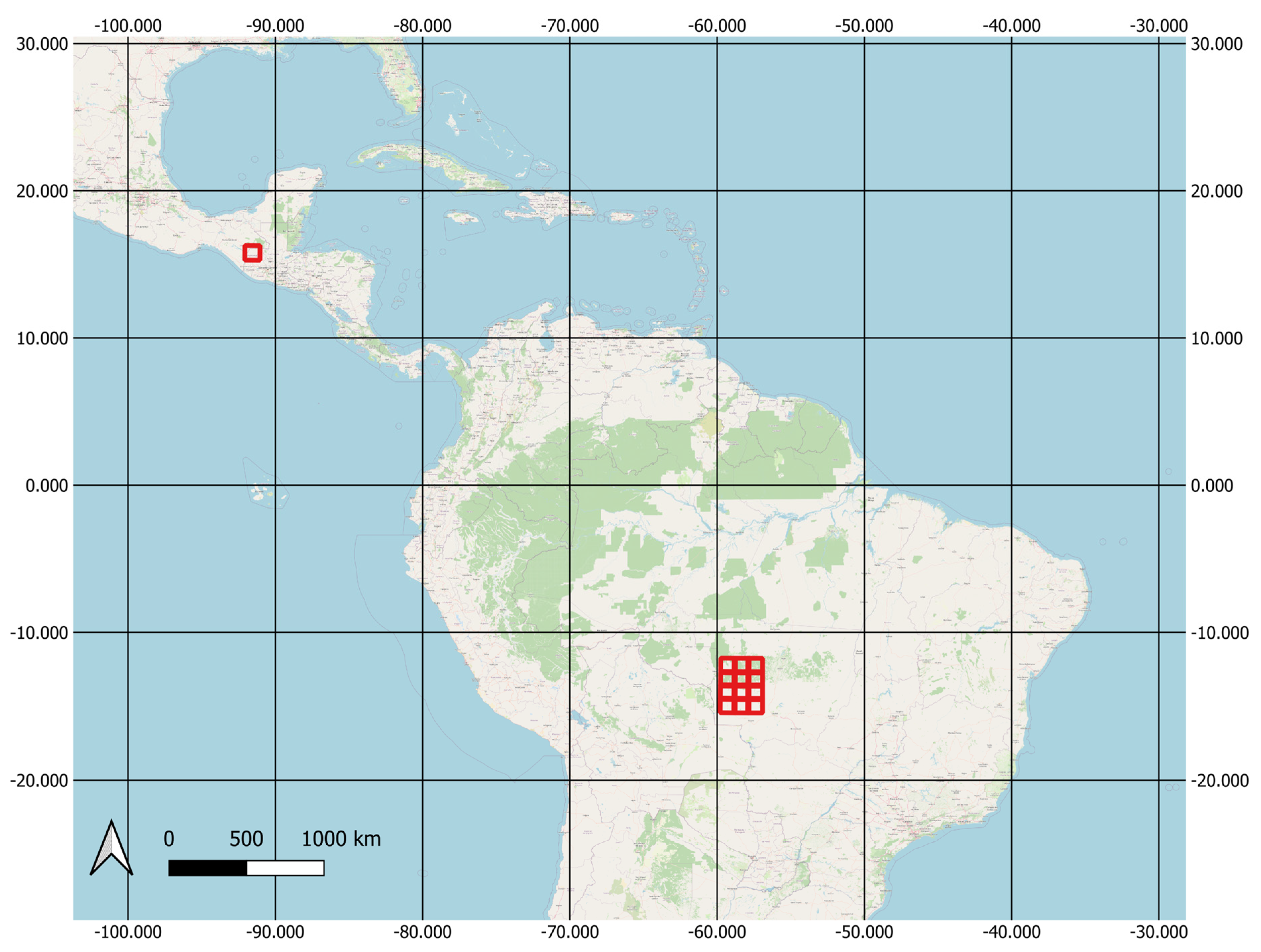
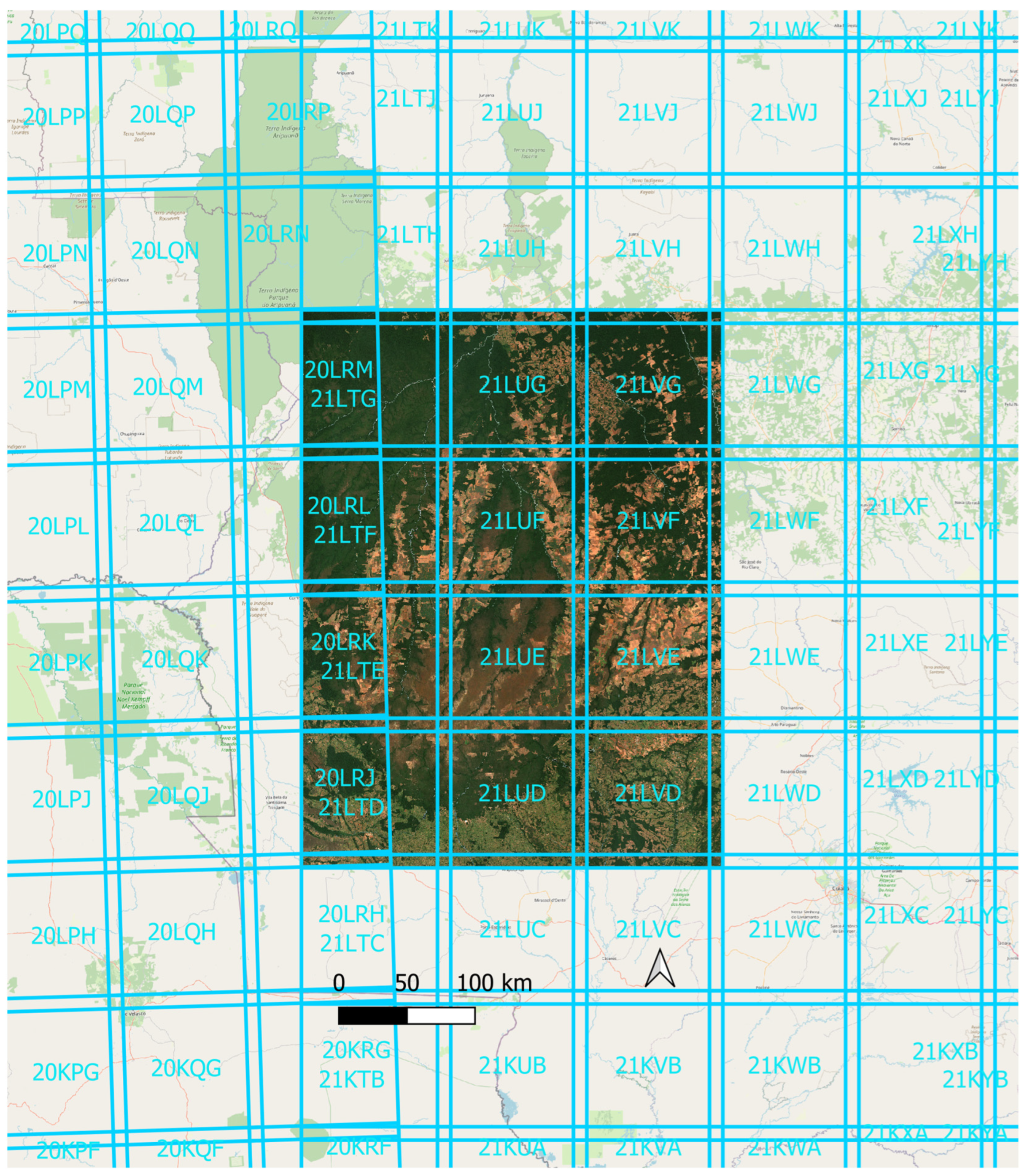
2.1. Study Areas

The study areas were located in nine Sentinel-2 tiles in Mato Grosso State in Brazil and in one 100 km × 100 km Sentinel-2 tile in Guatemala (Figure 1). Guatemala is a major coffee exporter. The State of Mato Grosso exports primarily soybeans, but also timber, meat, and cotton. Historically, forest clearance has served the expansion of cattle ranching and agricultural production, which constitutes the largest part of Mato Grosso’s economy.

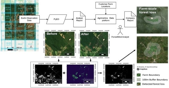
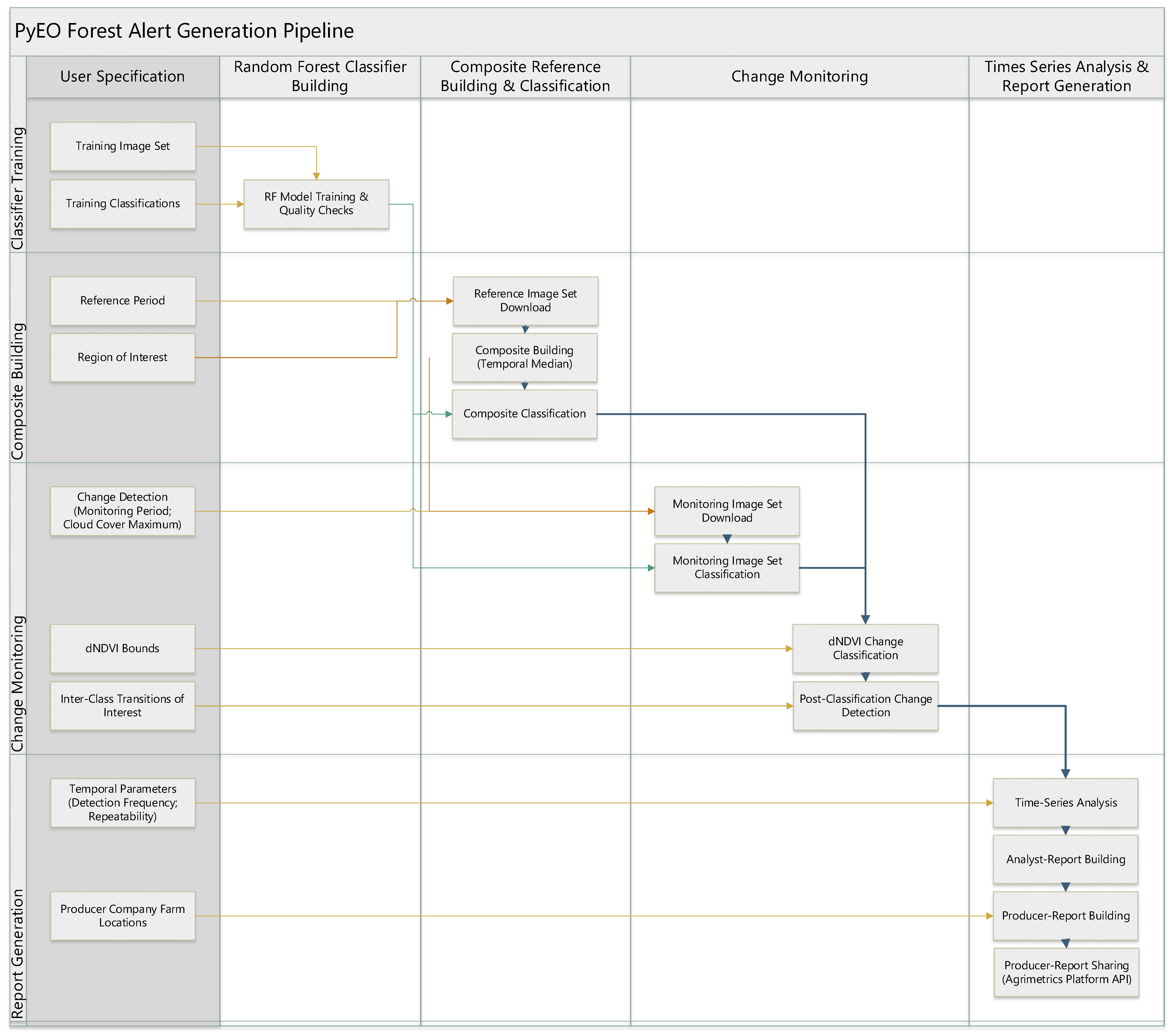
2.2. Software Development and Image Analysis

The software package developed in the ForestMind project for monitoring deforestation extends the capabilities of the Python for Earth Observation (PyEO) package [14,19]. PyEO was developed primarily as an implementation of automated near-real-time satellite image processing chains to provide timely forest alerts, which show forest cover loss detections based on two land cover maps that have been classified by a trained machine learning model. PyEO contains many useful generic functions that can also be used for other image analysis and change detection tasks. As a source of imagery, Sentinel-2 products are currently supported as the primary data source, but other satellite constellations such as Planet and Landsat have been used in past trials. Sentinel-1 Synthetic Aperture Radar (SAR) images could be accommodated within the same framework in future developments. Working from the Sentinel-2 image data stream, PyEO can deliver forest cover loss alerts every 5 days at 10 m spatial resolution, subject to possible occlusion by cloud cover and haze in the imagery.

A flowchart of the PyEO-based image processing pipeline is given in Figure 2. For ForestMind, we introduced several methodological developments to our earlier PyEO forest alerts algorithm [14] to meet the project’s requirements. These are described below. The version of PyEO in this paper has been released as the ‘ForestMind Extensions’ of PyEO, version 0.8.0 on GitHub (https://github.com/clcr/pyeo/releases/tag/v0.8.0, accessed on 27 November 2023) and Zenodo [20].

The machine learning approach taken in this work has evolved from earlier work [14]. Previously, change detection was based on direct, single-step differential detection of transitions between land cover classes by classifying forest change directly based on a vector of spectral reflectances from two time points from image pairs with a random forest classifier. The classifier was trained, pixel by pixel, on examples of inter-class land cover changes, such that a class label could be ‘forest cover to non-forest cover’ between the image pairs, for example. In practice, however, the relatively rare nature of the forest cover loss classes in some areas made it very difficult to collect consistent, high-quality training data to provide good coverage over all transitions of interest—ultimately limiting change detection capability. Creating a multi-temporal training dataset was challenging and time-consuming because it is harder to visually find areas of a particular type of change. A single image is much easier to understand by a human interpreter. Based on this experience, the PyEO forest alerts algorithm now adopts a direct classification of land cover classes (instead of land cover change classes), followed by post-classification change detection through cross-tabulation of land cover classes at times 1 and 2.

First, a baseline image composite is created over a user-defined reference period. The composite is then classified into a land cover baseline map. For the change detection, a sequence of more recent single Sentinel-2 images is downloaded and classified into single-date land cover maps using the same model. A post-classification change detection process then compares the land cover class of the baseline composite to those of each change detection image to detect land cover changes.

To provide robustness to the effect of clouds, the PyEO forest alerts algorithm masks out clouds and cloud shadows based on the Scene Classification Layer (SCL) provided as part of the Sentinel-2 product. The cloud mask can optionally be dilated by applying a morphological filter to mask out the fringes of clouds and cloud shadows in neighbouring pixels.

To support this revised machine learning approach, a standardised set of land cover classes were defined (

Table 1. Generic specification of land cover classes that can be used in the change detection algorithm. Classes shown in italics were not used in the model training for this specific application and are only shown for completeness.

Class Number	Description
1	Primary forest
2	Plantation forest
3	Bare soil
4	Crops
5	Grassland
6	Open water
7	Burn scar
8	Cloud
9	Cloud shadow
10	Haze
11	Sparse woodland
12	Dense woodland

) and used as the basis for training the machine learning model using manually defined polygons of known land cover types.

In the evaluation of the forest cover loss detections from the post-classification change detection with the random forest model, under certain circumstances, forest cover loss was confused with spectrally similar landscape features. An example is a case of hillsides illuminated by the sun. To improve the quality of the forest cover loss detections, an optional additional classification test was introduced to the change detection process. When a change between a single-date Sentinel-2 image and the baseline image composite is detected, the difference in their Normalised Difference Vegetation Index (dNDVI) is calculated for each pixel. dNDVI is a measure of the decrease in vegetation greenness, which is often related to the loss of vegetation cover. The resulting dNDVI image can then be classified into two classes based on a simple threshold to create a map of areas where forest loss is likely to have occurred. Based on visual histogram analysis of dNDVI images of forest and non-forest areas, a dNDVI threshold of −0.2 was adopted as a default for generating this map. The output from this step is a hybrid change detection. Switching on this hybrid change detection option combines the change detections from dNDVI with the machine learning outputs through a logical AND operation with the aim to produce fewer false positive forest loss detections and a higher-quality change map.

Once the hybrid post-classification change detection has been performed for each Sentinel-2 change detection image relative to the baseline composite, a time-series analysis of the resulting sequence of binary change images (forest loss/no forest loss) is performed to build the analyst report as a multi-layered GeoTIFF file. The analyst report layers are updated when a new monitoring image is processed by the pipeline and contain aggregated information for each pixel, including the date of the earliest change detection, the number of confirmed subsequent change detections, the consistency of any change detection over time, and, derived from these, a binarised output layer that can quickly guide the analyst to the most likely areas of forest loss.

Following the image analysis stage, Python interfacing with the API of the Agrimetrics agricultural data-sharing platform was used to disseminate the resulting analyst reports across the ForestMind project team to make them available for assessment by forest analysts. Figure 3 illustrates the overall workflow by showing how the PyEO forest alerts form a component of the wider system.

The report data uploaded to the Agrimetrics platform are queryable via a RESTful API, which allows the deforestation information surrounding each farm to be requested automatically by a Python script. Based on such queries from Agrimetrics, company reports were compiled using a series of Python scripts executed in a Jupyter notebook by the ForestMind Analysts. The company reports made use of point or polygon data which indicated the precise location of farms as shared by the particular company. The resulting company report for customers was presented at farm scale, i.e., a tabulated row for each of their farms providing an approximate measure of deforestation surrounding the farm in hectares, a summary of calculated statistics, and a created overview map.

2.3. Model Training

To train the machine learning model for the random forest classification of land cover types, Sentinel-2 image composites were created for 12 Sentinel-2 tiles (

Table 2. List of Tile IDs of the Sentinel-2 image composites used for training the random forest model ‘mato_rf_toby_1’. All image composites were made from the median bottom-of-atmosphere radiance of the RGB and NIR bands at 10 m resolution from the 30 least cloud-covered images acquired during the calendar year 2019.

Granule ID
T21LTD
T21LTE
T21LTF
T21LTG
T21LUD
T21LUE
T21LUF
T21LUG
T21LVD
T21LVE
T21LVF
T21LVG

) from the least cloud-covered images acquired in the calendar year 2019 over Mato Grosso (Figure 4). Each tile has an area of 100 km × 100 km = 10,000 km². To collect training data, polygons of known land cover types were visually delineated using the QGIS geographic information system [21] and a land cover class was assigned to the attribute table (Table 1).

The training polygons were saved in a shapefile for each Sentinel-2 image tile. During the model training step, all polygons from all Sentinel-2 image composites across the 12 tiles were read into a data table together with their assigned land cover class codes and rasterised to the Sentinel-2 spatial resolution of 10 m. Random forest model training was carried out for 500 decision trees with the scikit-learn library [22], and the trained model was saved to a Python standard pkl file.

In total, 75% of the training pixels were used for random forest model training, and 25% were held back for validation. An initial model training with all pixels from all polygons resulted in a low classification accuracy of 56% for the independent validation pixels, even though the accuracy of the 75% training pixels was 99.9%. The distribution of training pixels by class was found to be heavily unbalanced: class 1 had 1,708,257 training pixels, class 3 had 1,464,283, class 4 had 838,431, class 5 had 57,269, class 11 had 540,293, and class 12 had as few as 36,085 training pixels. To achieve a more balanced distribution of training pixels per class, a limit of a factor of 10 in the sample size ratios was introduced. From each land cover class that had more than 10 times the number of training pixels compared to the least frequent class, a random sample of pixels was drawn; in this case, 360,850 pixels. This more balanced random forest classification model achieved a validation accuracy of 92.8% when compared to the 25% of independent validation pixels, and 99.9% for the 75% of pixels that were used to train the model.

The feature importance f of the model shows that band 4 was the most important spectral band for discrimination of the land cover types (f₄ = 0.38), followed by band 8 (f₈ = 0.29), band 3 (f₃ = 0.19), and band 2 (f₂ = 0.13).

Table 3. Confusion matrix of the balanced random forest classification model from the comparison with the 25% of training pixels that were held back for the independent validation. UA = User Accuracy, PA = Producer Accuracy, OA = Overall Accuracy.

	Reference Class →
Predicted Class ↓	1	3	4	5	11	12	UA ↓
1	84,955	2	210	56	4650	9	94.5%
3	0	87,159	1092	109	1017	524	96.9%
4	73	1332	85,147	1977	611	1250	94.2%
5	53	93	2000	11,005	959	272	76.5%
11	4730	650	374	545	84,214	87	93.0%
12	53	871	2958	534	508	4110	45.5%
PA →	94.5%	96.7%	92.8%	77.4%	91.6%	65.7%	OA = 92.8%

shows the confusion matrix and

Table 4. Spectral signatures of the training classes for the four selected Sentinel-2 image bands derived from the random forest model ‘mato_rf_toby_1’. Sentinel-2 bands: 2 = B, 3 = G, 4 = R, 8 = NIR.

Class	Band	Min	Max	Mean	Stdev
1	2	74	668	207.49	31.83
	3	130	1130	398.40	57.63
	4	86	1352	229.00	49.20
	8	912	5144	2726.92	371.26
3	2	211	2113	477.09	216.21
	3	391	2655	741.56	279.71
	4	323	3348	1034.24	453.30
	8	1160	4087	2246.23	632.23
4	2	203	1872	415.48	97.21
	3	411	2334	724.29	145.90
	4	267	2837	621.16	241.67
	8	1723	5684	3644.23	646.96
5	2	184	771	429.65	106.77
	3	340	1129	771.52	154.28
	4	214	1393	746.34	237.52
	8	1742	4003	2813.10	311.96
11	2	146	626	300.66	55.23
	3	298	914	536.95	62.15
	4	176	1214	430.51	145.68
	8	1530	4324	2468.49	289.34
12	2	189	906	466.51	99.30
	3	361	1336	774.15	133.53
	4	225	1798	815.29	240.96
	8	1320	4628	2897.72	362.87

the spectral signatures of the classes from the training data. The achieved accuracy of 92.8% was considered sufficiently high to use this model in the due diligence application.

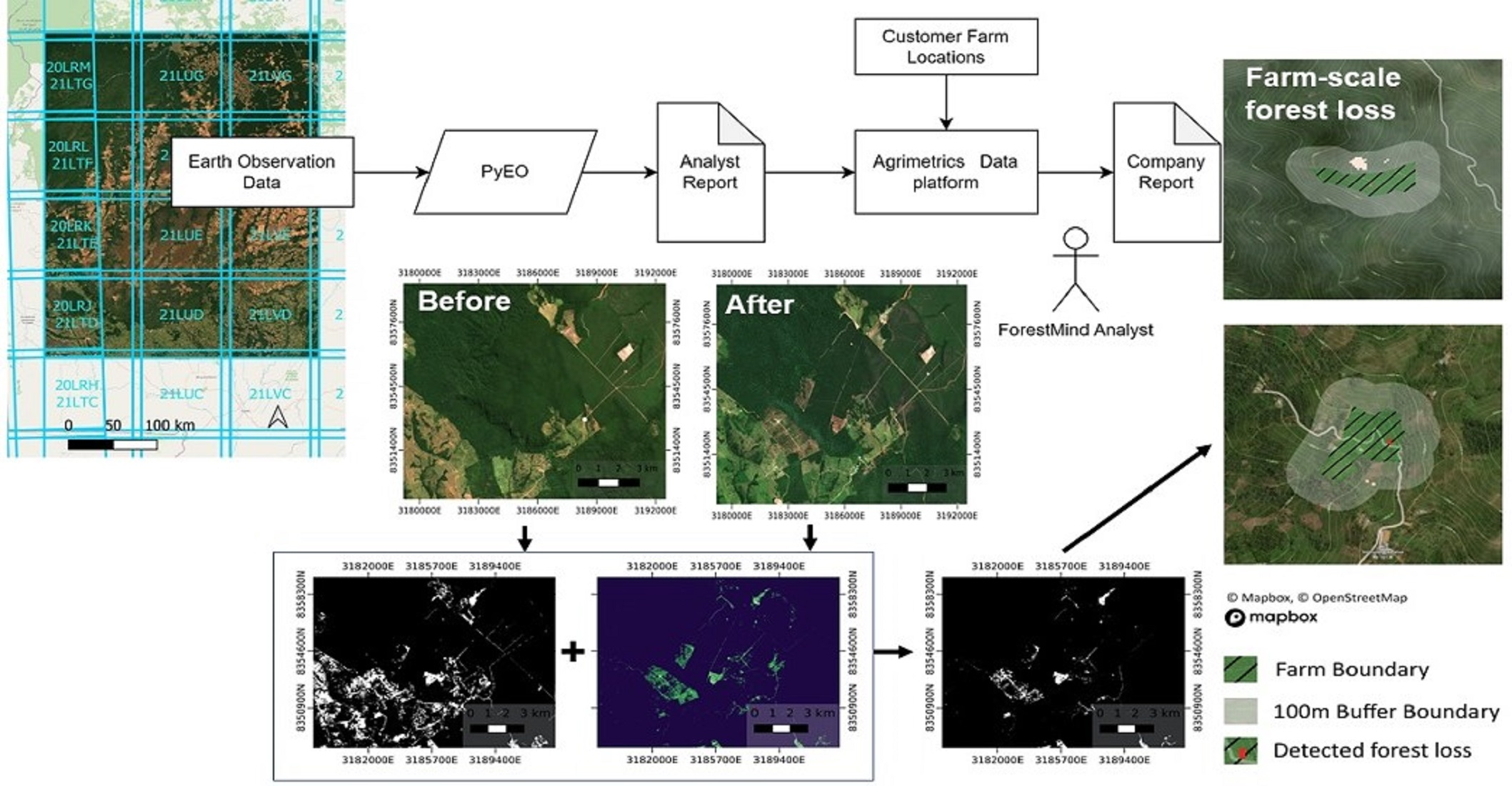
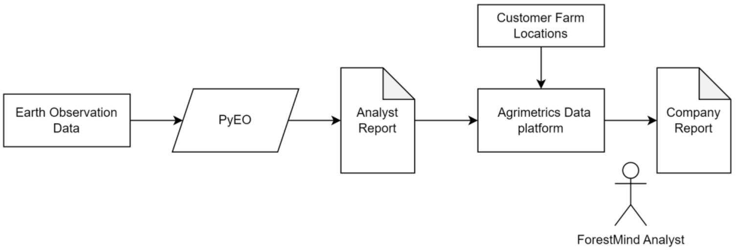
2.4. Pilot Operational Application

A pilot period was run in operational production mode from January to August 2022 during which company reports were generated monthly in step with the forest cover loss analyst reports being updated with the latest Sentinel-2 change detection images. These reports incorporate farm location data obtained from UK coffee importers with the aim of detecting and reporting on any forest cover loss happening in the vicinity of the farms as part of their environmental due diligence. The data supplied by the coffee importer were in the form of point locations, recorded by handheld GPS devices. Polygons for the farm extent were not available as the importers had not collected these data.

3. Results

This section reports on the forest cover loss detection results from Sentinel-2 for a region in the Huehuetenango Department, Guatemala, and another region in the State of Mato Grosso, Brazil. The presented forest cover loss maps were generated from a baseline image composite for the reference year 2019 compared to change detection images from Sentinel-2 acquired from January to August 2022. Multiple such change detections are aggregated into a raster file (the analyst report) incorporating a number of ‘report layers’ of spatial information about each pixel in the raster. These reports are designed to be easily understandable by non-experts and are intended to be used to demonstrate due diligence by importers and exporters to show that their trade does not inadvertently cause deforestation in the source regions of their produce.

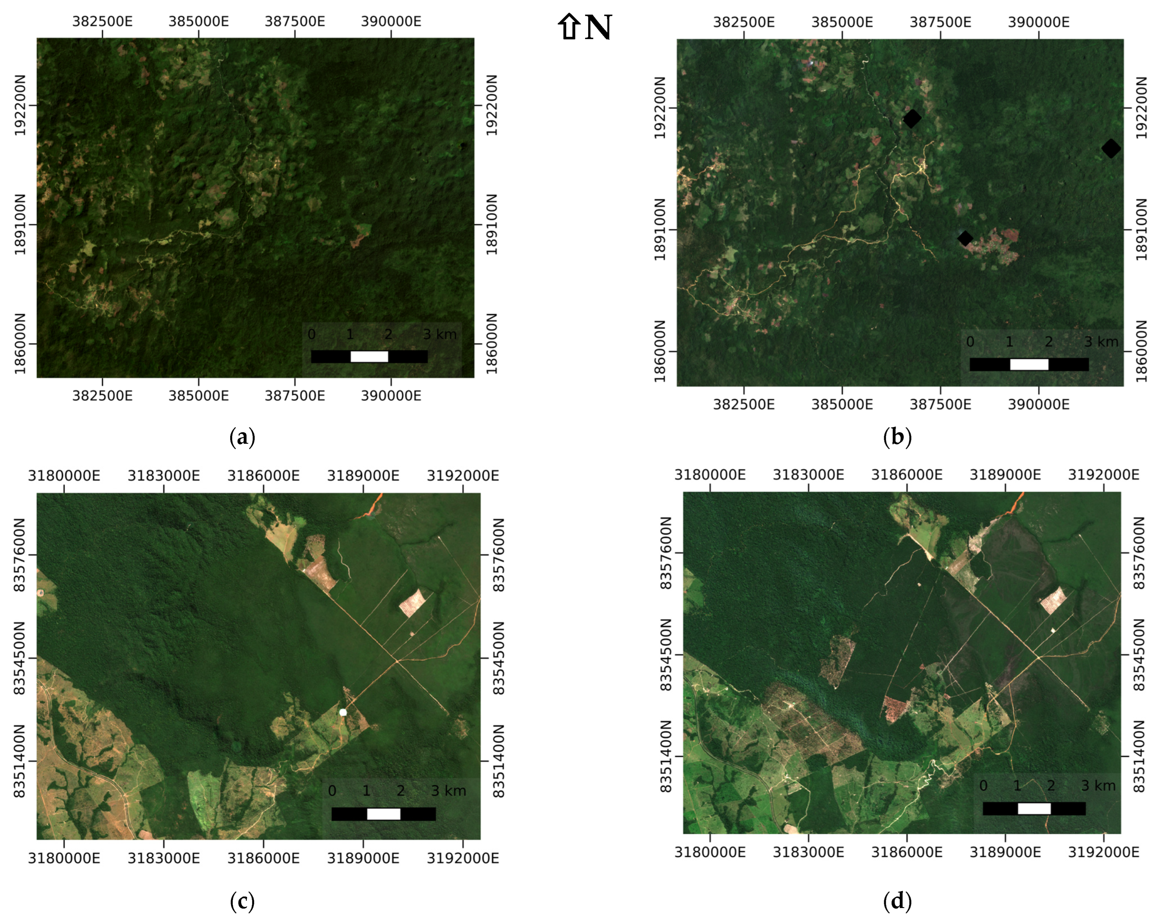
3.1. Median Image Composite Creation

Figure 5 shows the median composites for a Sentinel-2 tile in Guatemala and Mato Grosso derived from cloud-free images acquired in 2019 with cloud cover <10%, and the corresponding sample change detection images acquired in July 2022 for Guatemala and April 2022 for Mato Grosso.

The image composites were created by calculating the median of a stack of images (Sentinel-2 L2A products) of atmospherically corrected surface reflectance for each band, excluding missing values, cloud-masked pixels, and cloud-shadow-masked pixels. By comparing the composites on the left of Figure 5 to the sample images on the right, areas of forest loss are recognisable to a human observer given the change in colour of the RGB channels shown.

3.2. Near-Real-Time Image Query and Download Functionality

Images with more than 10% cloud cover were discarded from the download and change detection algorithm because visual inspection showed that their radiometric quality tends to be poor due to remaining cloud fragments, haze, and cloud shadow areas. Altogether, 30 images were downloaded for the Guatemala tile and 63 for the Mato Grosso tile. Where L2A surface reflectance images were available on the Copernicus Open Access Hub, they were downloaded. If only L1C top-of-atmosphere radiance image products were available, they were downloaded and atmospherically corrected with Sen2Cor as part of the PyEO workflow.

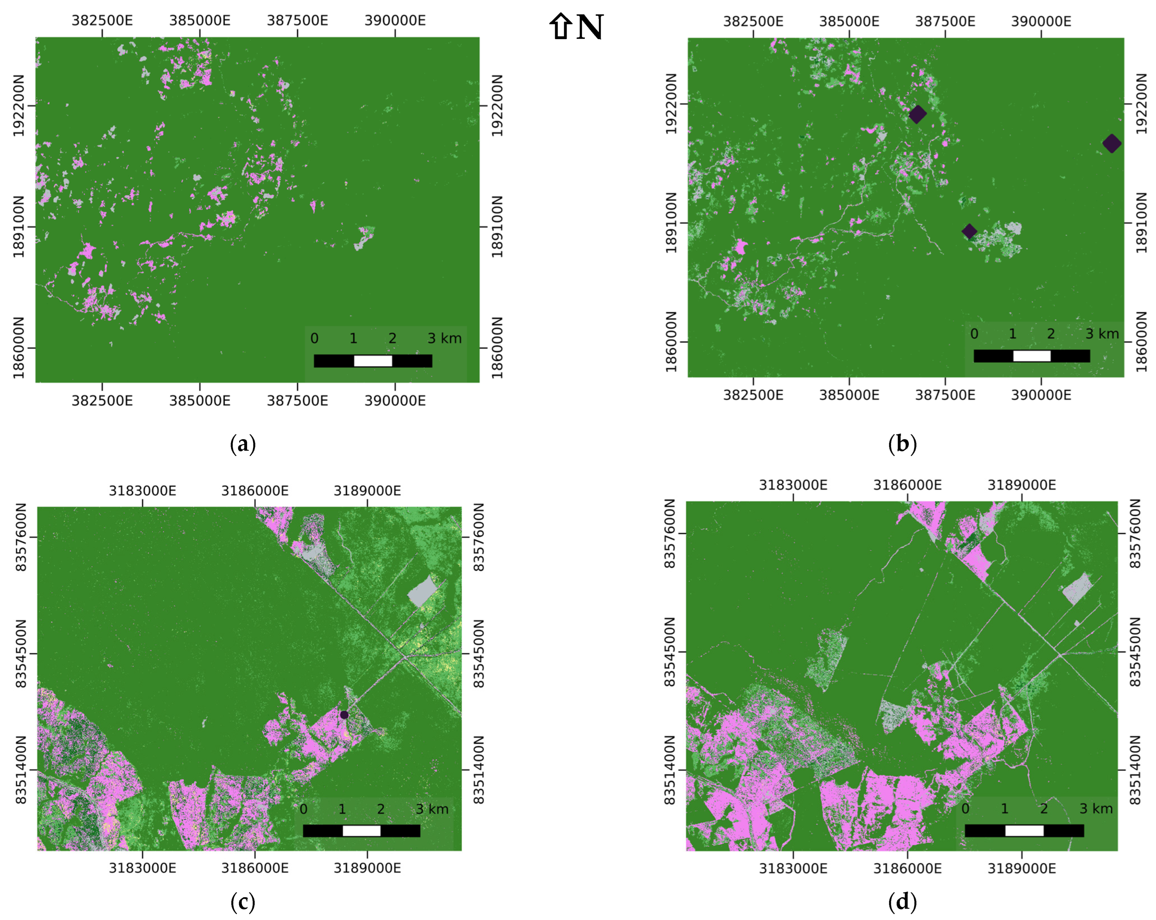
3.3. Random Forest Classifications

Figure 6 shows an example of a random forest classification of the land cover types in Table 1 for the Guatemala and Mato Grosso tiles. The same random forest model was applied consecutively to the baseline image composite from 2019 and all change detection images for the near-real-time change detection period between January and June 2022.

3.4. Post-Classification Change Detection

Figure 7 shows sample results of post-classification change detection for the Guatemala and Mato Grosso tiles. The change maps were derived by identifying all transitions from any of the forest classes 1 (primary forest), 11 (sparse woodland), and 12 (dense woodland) to any of the non-forest classes 3 (bare soil), 4 (crops), or 5 (grassland) using a purpose-built function from the PyEO library. Class 2 (plantation forest) was not included in the forest classes because rotation forestry was not a change of interest in the change detection step.

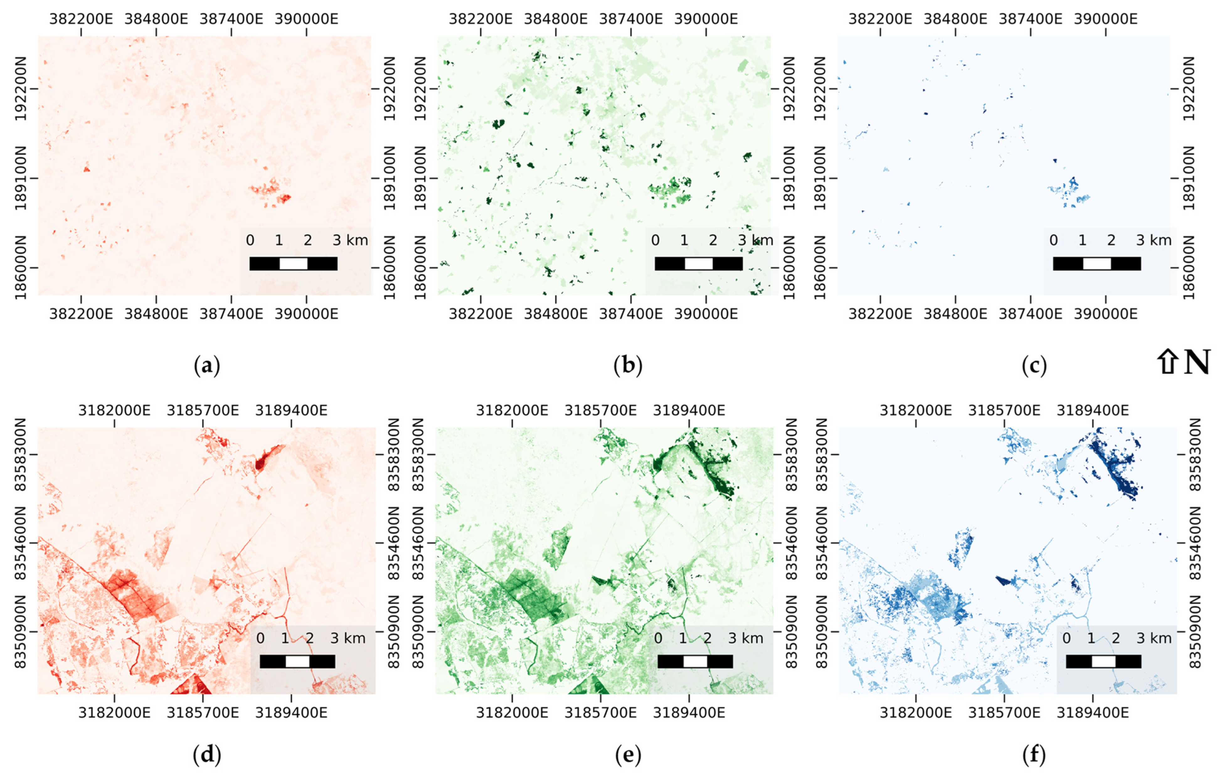
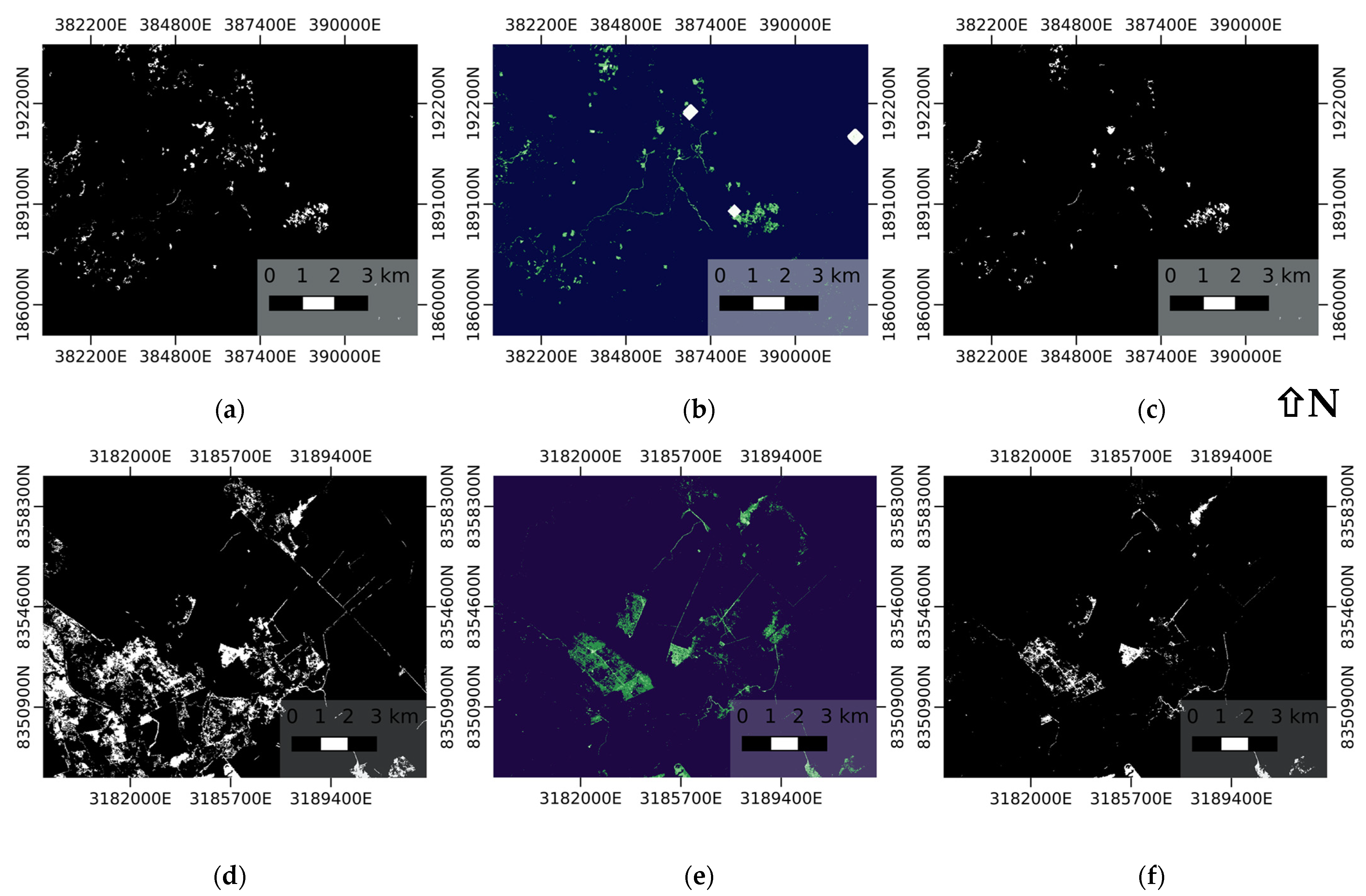
3.5. dNDVI Change Thresholding to Create Hybrid Change Detections

As described in the methodology section, a hybrid classification option was applied, whereby the random forest post-classification change detection was supported by a secondary classification of pixels as being potential areas of forest loss based on a measured change in NDVI of at least dNDVI < −0.2 relative to the baseline image composite.

Figure 8 shows the results of the post-classification change detection. The hybrid change detection method removes some agricultural areas that have been misclassified from the change detection maps and results in cleaner forest loss maps with less noise.

3.6. Time-Series Analysis and Aggregation into the Analyst Report

The analyst report consisted of a multi-layer GeoTIFF image (Figure 9) containing aggregated information extracted from the time series of hybrid change detection maps. It is updated whenever a new change map is created. The analyst report was uploaded to the Agrimetrics platform, which provided a centralised database for the ForestMind consortium. The analyst report product can be read by the QGIS software package to allow convenient viewing and analysis of the information layers (Here, QGIS version 3.28.15 was used). The reports comprise seven raster layers with information about each pixel:

• Layer 1 ‘First_Change_Date’: The acquisition date of the Sentinel-2 image in which a change of interest (i.e., forest loss) was first detected. This is expressed as the number of days since 1 January 2000;
• Layer 2 ‘Total_Change_Detection_Count’: The total number of times when a change was detected since the First_Change_Date for each pixel;
• Layer 3 ‘Total_NoChange_Detection_Count’: The total number of times when no change was detected since the First_Change_Date for each pixel;
• Layer 4 ‘Total_Classification_Count’: The total number of times when a land cover class was identified for each pixel, taking into account partial satellite orbit coverage and cloud cover;
• Layer 5 ‘Percentage_Change_Detection’: The computed ratio of Layer 2 to Layer 4 expressed as a percentage. This indicates the consistency of a detected change once it has first been detected and thus the confidence that it is a permanent change rather than, for example, seasonal agricultural variation or periodic flooding;
• Layer 6 ‘Change_Detection_Decision’: A computed binary layer that is set to 1 to indicate regions that pass a change detection threshold and so allows regions of significant change to be rapidly identified over the large spatial area of a tile. Currently, the decision criterion is that ((Layer 2 >= 5) and (Layer 5 >= 50)), i.e., that at least five land cover changes of interest were detected and that the change was present in at least 50% of the change detection images;
• Layer 7 ‘Change_Detection_Date_Mask’: A subset of First_Change_Date only showing those areas where the change decision criteria were met. It is the product of Layer 1 and Layer 6. This allows regions where land use change is expanding over time to be more easily identified over the large spatial area of a tile.

In practice, report image Layer 7 is used to provide information on areas that require rapid attention. Layers 2 and 5 provide additional information on the severity and timing of land cover change events to support decision making on whether to flag a forest loss for follow-up investigation.

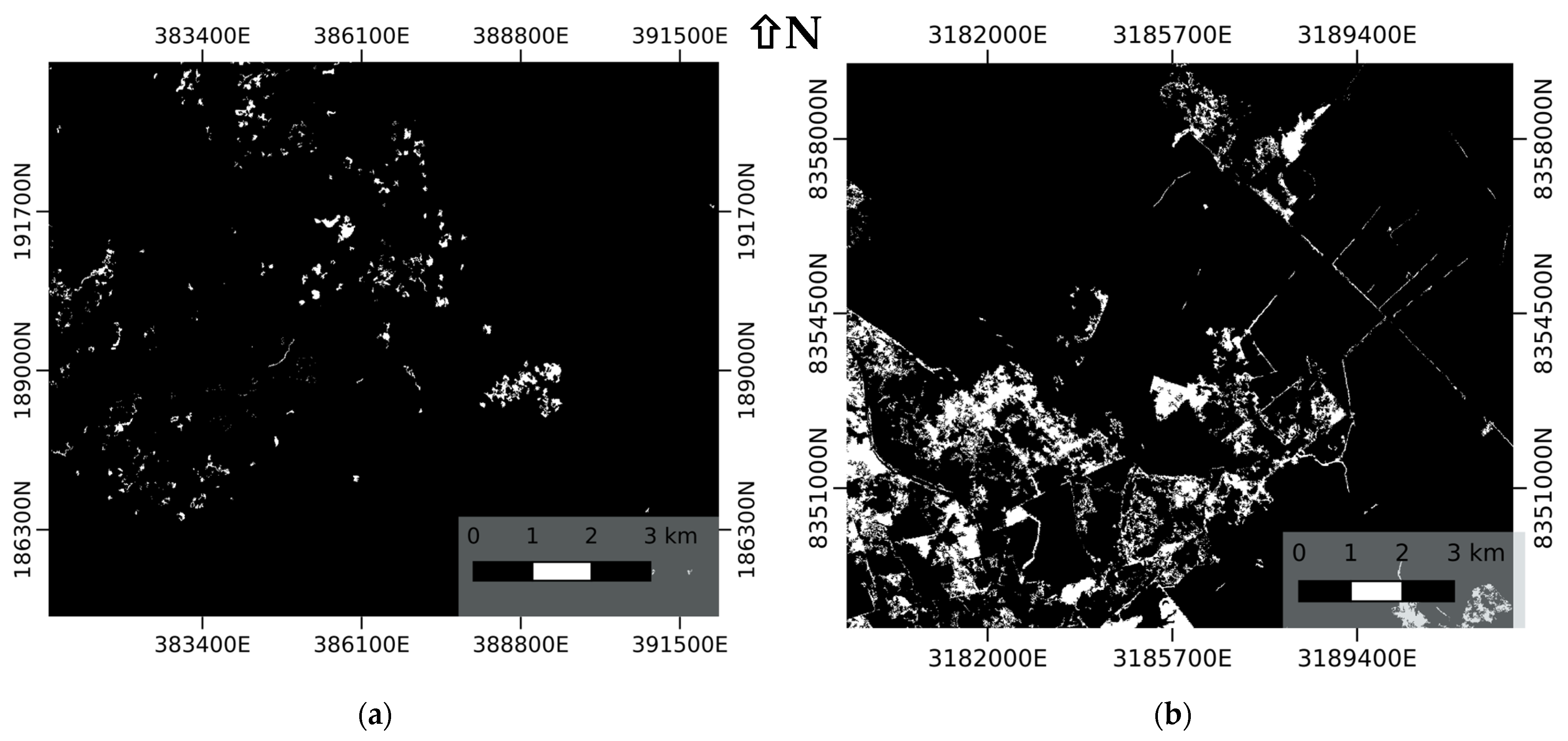
3.7. Validation of the Forest Loss Detections

To validate the observed forest loss detection in Guatemala and Mato Grosso, a stratified random sampling method was used, as described by Cochran [23], at the scale of the processed Sentinel-2 tiles. Two main strata were selected in Guatemala and Mato Grosso, comprising areas of forest cover loss and unchanged forest. In addition, a third stratum was defined that included areas of potential forest loss around the identified forest change. This zone serves to reduce omission errors that may occur in vegetative transition zones and around large strata [24,25,26]. An inner zone of potential forest loss of 20 m (i.e., 2 pixels) was defined around the areas of forest change to reduce omission errors during validation. A total of 600 stratified random points (200 points per stratum) per area were examined, and accuracy metrics, including Cohen’s Kappa [27], were calculated. Visual validation was carried out by interpreting a pair of before and after images around the time of the first detection of the forest loss, as well as for a stratified random sample of unchanged forest areas for comparison.

The accuracies of the forest loss detections in Guatemala and Mato Grosso for the period 2019 to 2022 were quantified as 86.3% and 85.5% overall accuracy, respectively (

Table 5. Confusion matrices showing the forest loss detection algorithm’s overall accuracy of the forest change detections and the areas of no detected change, stating user accuracy, and producer accuracy in Guatemala (top) and Mato Grosso, Brazil (bottom), between 2022 and a median image composite of 2019. OA = overall accuracy, κ = kappa coefficient.

Guatemala OA = 86.3% κ = 0.71	No Change	Change	User Accuracy
No Change	193	7	96.5%
Change	48	152	76%
Producer Accuracy	80.1%	95.6%
Mato Grosso, Brazil OA = 85.5% κ = 0.72	No Change	Change	User Accuracy
No Change	187	13	93.5%
Change	45	155	77.5%
Producer Accuracy	80.6%	92.3%

). About 229,140 ha of forest in Guatemala and 110,480 ha of forest in Mato Grosso were lost between 2019 and the first half of 2022, while about 442,196 ha and 295,927 ha of forest remained unchanged. Forest change patches were distributed throughout the areas of interest, with most patches concentrated along forest edges. The patch sizes of forest changes in Guatemala ranged from 0.01 ha to 7011.89 ha and for Mato Grosso from 0.01 ha to 12,846.41 ha.

The use of zones of potential forest loss around the forest loss detections increased the accuracy of the validation for Guatemala and Mato Grosso by 2.4% and 3.5%, respectively. These differences in accuracy reflect the importance and effectiveness of the buffer method and are consistent with previous findings that showed an increase in validation accuracy [25,28]. Finally, for Mato Grosso, the kappa coefficient was κ = 0.71, and for Guatemala, κ = 0.72, showing a ‘substantial agreement’ according to Cohen’s interpretation [27]. Cohen suggested that κ values ≤ 0 showed no agreement, 0.01–0.20 showed none to slight agreement, 0.21–0.40 a fair agreement, 0.41–0.60 a moderate agreement, 0.61–0.80 a substantial agreement, and 0.81–1.00 almost perfect agreement.

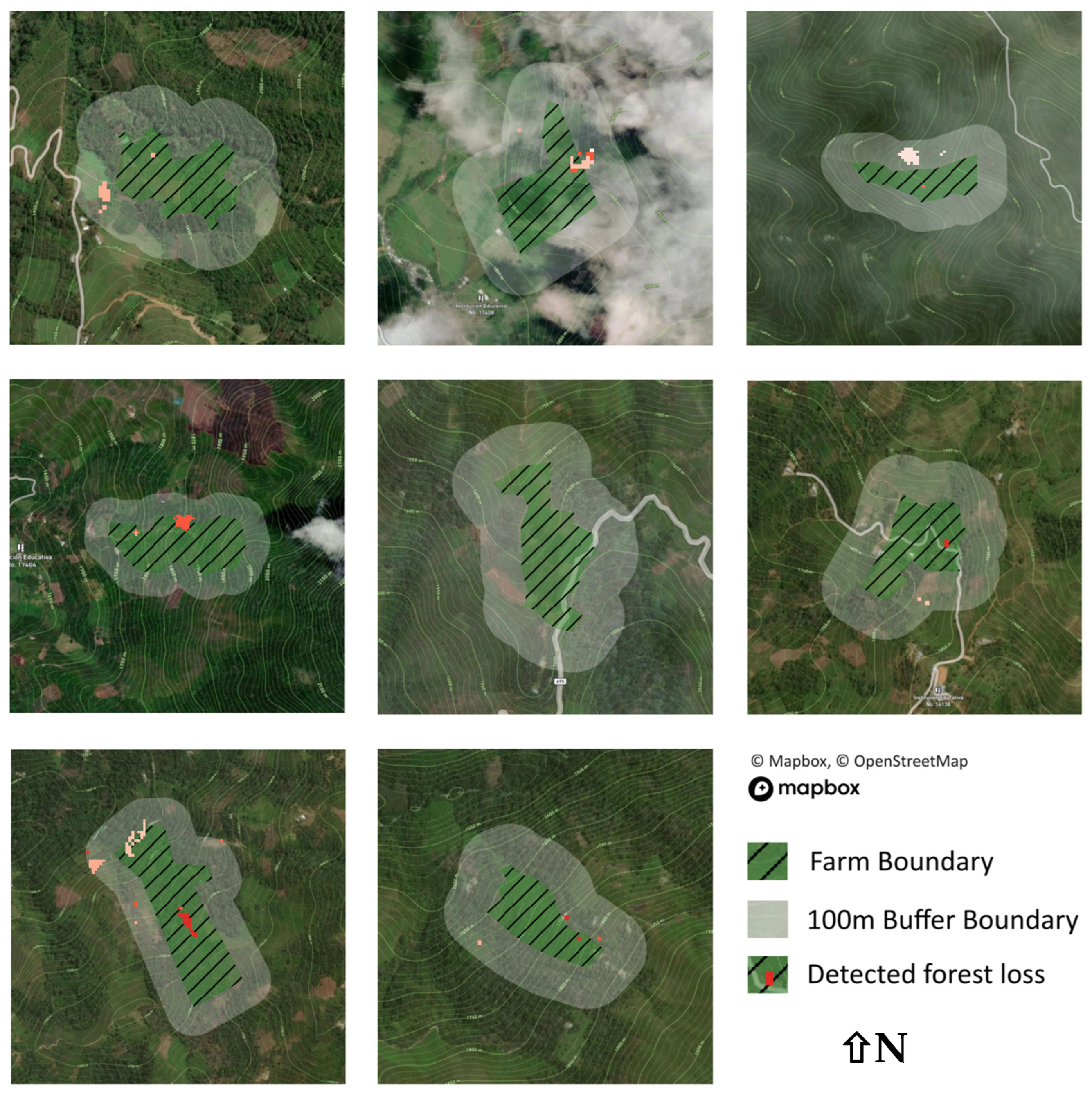
3.8. Independent Validation of Farm-Scale Change Detection Accuracy

In addition, a combination of Sentinel-2 imagery and monthly <5 m resolution data from Planet Norway’s International Climate and Forests Initiative (NICFI) was used to validate the points. For this purpose, an image before the forest loss detection and a second image after the detection were interpreted visually for evidence of forest loss. Validation of forest change in Guatemala was carried out using imagery from April 2022, and validation of forest change in Mato Grosso using imagery from August 2022. Validation of the deforestation detections was carried out at the Satellite Applications Catapult by visual inspection of the forest loss detections presented in this paper compared to the Global Forest Watch data [13]. Planet NICFI data were used for this purpose. These results are presented separately, as this was an independent validation by a team not involved in producing the forest loss dataset.

In order to gather feedback from users on the supply chain monitoring reports, forest loss detections from the PyEO algorithm were analysed for a set of real farms from which commodities are imported by one of the ForestMind user organisations. For every user organisation, a farm-scale map was created, showing data within 400 m of its location, together with information on the extent of forest cover loss (Figure 10,

Table 6. Forest cover loss detections in the areas of the real farms for the two reporting periods (the baseline and baseline update), and summarised for the whole monitoring period.

Period	Total Number of Farms	Deforestation-Free Farms	Farms with Deforestation < 0.1 ha	Farms with Deforestation > 0.1 ha
Jan 2020–Jan 2022 (Baseline Update)	263	155	94	14
Jan 2022–Aug 2022	263	149	113	1
Jan 2020–Aug 2022 (Whole Monitoring Period)	263	105	136	22

). In addition, statistics about the proximity of the farm to protected areas and/or rivers were made available to the users.

In total, 263 farms were examined through the ForestMind monitoring period from January 2020 to August 2022, of which 105 were reported as ‘deforestation-free’, 136 were found to have only minimal deforestation (<0.1 ha), and 22 were found to have larger areas of deforestation (>0.1 ha).

Throughout the project lifecycle, the datasets generated by ForestMind were assessed for accuracy. In the absence of regularly updated ground data for the region, a visual assessment was carried out using 3 m resolution Planet-NICFI (Norway’s International Climate and Forests Initiative) data, which are openly available, as well as a comparison with the existing annual dataset of forest loss, Global Forest Loss from the University of Maryland based on Landsat imagery, available via Global Forest Watch [13].

For each forest loss dataset, 100 points were randomly selected from two classes: those classified as having forest loss and those not classified as experiencing forest loss. The two datasets for assessment are as follows:

• PyEO Forest Loss—this study, University of Leicester (7 February 2019–22 February 2021);
• Global Forest Loss—University of Maryland (2017–2020).

Each dataset was visually inspected using the Planet-NICFI data, looking at a time series of imagery from before and after the date on which forest loss was detected. Statistics generated are commission (change detected when no change occurred) and omission error (change not detected when change occurred), as well as the overall accuracy percentage. In August 2022, a final accuracy review of the forest loss detections was carried out. The datasets were tested in the two different regions of Mato Grosso in Brazil, for which the random forest model had been trained, and Guatemala, as a study area to which the model was transferred to test its applicability elsewhere. The State of Mato Grosso in Brazil is known for the growth of soybeans and the area of Guatemala for coffee. The results are presented in

Table 7. Accuracy, commission, and omission rates for forest loss vs. visual assessment of Planet NICFI datasets at farm scale of the real farm locations. The producer accuracy is 100%, rate of omission, and the user accuracy is 100%, rate of commission.

Dataset	Overall Accuracy	Rate of Commission	Rate of Omission
PyEO forest loss— Soy Brazil	83%	18%	1%
PyEO forest loss— Coffee Guatemala	80%	21%	3%

.

4. Discussion

The technical algorithm of forest cover loss detections from the PyEO package has been described previously in the literature [14,15]. This study presents the ForestMind extensions of PyEO, which now includes an optional verification of detected forest loss pixels with a dNDVI threshold, which reduces the commission error greatly when run in entirely automatic mode.

Creating farm-scale company reports that clearly communicate farm forest cover loss rates for deforestation assessments to non-technical companies to provide actionable information was challenging. Feedback from the initial report indicated that the customer ‘felt unclear’ about the information provided and the next steps. Specific feedback included the structuring of the report to ensure that the most relevant data were easily understandable and accessible at a glance. Subsequent reports were improved by restructuring the text and providing clearer labelling, explanations, and legends. In the later versions of the report, the feedback ranged from ‘felt somewhat clear’ to ‘felt very clear’ (n = 3). The customer still experienced some difficulties interpreting the data in these reports. This was primarily because of the need to learn to interpret spatial data presented in the reports. Because the due diligence requirement is a new legal instrument, companies have yet to learn how to use evidence-based due diligence systems in their supply chains. Backdrop imagery greatly supported the visualisation of the change detections, but at the scale of a coffee farm (3–12 ha), 10 m resolution Sentinel-2 imagery is not suitable as a background map. The 3 m resolution imagery from Planet was also used, yet farm boundaries were still not clearly identifiable at this resolution. The final revision of the reports used a custom background map created in Mapbox Studio, which provides very-high-resolution commercial satellite imagery with additional contours, and streets overlain from OpenStreetMap, added by the analyst to support the visualisation. These data aided in the visual interpretation, though the background imagery suffered from misalignment, and was often out of date.

Whilst the accuracy of the forest loss detections allowed the production of a farm-level report based on an approximate point location for the farm without precise farm boundary data, the reports could not verify deforestation-free farm claims with high confidence. The reports communicated this limitation and suggested data collection exercises to improve the supply chain information held by importers and exporters. The customer companies considered these practical suggestions valuable, as they did not previously understand how the fidelity and precision of their supply chain information may impact their deforestation due diligence reporting. One customer responded, “At this stage whilst it brings important information and findings, and gives clear recommendations, these are currently known next steps for us as an organisation, albeit they are not easy next steps”.

The results of the two independent accuracy assessments at tile scale and at farm scale showed over 80% overall accuracy. Table 5 shows achieved user accuracies of the forest loss detections of 76% for Guatemala and 77.5% for Mato Grosso, and Table 7 shows 79% and 82% user accuracies for the two areas, respectively.

Previous studies have reported user accuracies of over 90% for the GLAD alerts from Landsat in a study in Peru [29], 97.6% for the RADD alerts from Sentinel-1 for disturbance events ≥0.2 ha in the Congo basin (but leaving a large number of small-scale forest losses undetected) [11], 71.1% (but only 53.3% for Latin America) for the JJFAST change detections [30], and over 97% for previous applications of PyEO forest alerts in Mexico and Colombia [15]. Differences in the spatial resolution of the satellite images, minimum mapping unit of the forest cover loss areas, study area characteristics, and detection methods complicate a direct comparison of the user accuracies of these previous studies. For example, the GLAD alerts have a 30 m × 30 m spatial resolution, which is an area nine times larger than the 10 m × 10 m presented here. Despite the GLAD alerts being a global system, the only published validation known to the authors is from Peru [29]. Pacheco et al. [15] compared the GLAD alerts with PyEO forest alerts for Mexico and Colombia and found that the GLAD alerts reported nearly four times more deforested area than PyEO for the site in Colombia, and missed a large number of small-scale forest loss areas in Mexico. The JJFAST validation [30] showed huge variations in users’ accuracies between study areas. In the context of previous forest loss detection studies, the results presented here are of acceptable accuracy for the purpose of automated change detection for ongoing due diligence reporting in the view of the authors.

In this study, we have presented two applications of the PyEO ForestMind reports to Guatemala and Mato Grosso State in Brazil. Could its application be scaled up to larger regions or continents, or a global scale? The forest types of the two regions studied here are similar enough for the random forest model that was trained on images from Brazil to work well in Guatemala. However, applying the same methodology to other forest types requires random forest models that were trained for specific forest conditions if their spectral reflectance properties are substantially different. A feasible approach might be to use a stratification of forests by ecoregion, as in Dinerstein et al. [31], and train ecoregion-specific models. The PyEO package already allows Sentinel-2 tile-based processing and can easily be scaled up to larger areas with sufficient computational resources. Hence, it has applicability in all forested or partially forested areas of the world. Its main strengths are that the customer can define their own land cover types and land cover change transitions of interest, train their own model, and receive change detections as often as desired, from the 5-day repeat cycle of Sentinel-2 to aggregated monthly or annual reports.

5. Conclusions

This paper introduces a technical solution to the due diligence obligations on importers and exporters to the EU single market under the EU Deforestation Regulation. It provides routine insights into forest cover loss around the areas of source farms in countries from which commodities are imported.

The analysis of the ForestMind reports from satellite imagery presented here demonstrates that automated forest loss detection algorithms can be customised by training a random forest model for the transition between land cover classes, or groups of classes, of interest and applied with very good accuracy.

The ForestMind farm-scale company reports on estimated deforestation rates offer a solution to suppliers of produce subject to the EU Deforestation Regulation and similar laws. While the data processing and visualisation are entirely automated with the help of the PyEO package, the farm-scale reporting does require human interpretation by a Forest Analyst to write a short narrative text about the data. However, AI solutions may in the future offer a means of automating this interpretation step.

References

1. Chakravarty, S.; Ghosh, S.; Suresh, C.; Dey, A.; Shukla, G. Deforestation: Causes, Effects and Control Strategies. Glob. Perspect. Sustain. For. Manag. 2012, 1, 1–26. [Google Scholar]
2. European Commission Green Deal: EU Agrees Law to Fight Global Deforestation and Forest Degradation Driven by EU Production and Consumption 2022. Available online: https://environment.ec.europa.eu/news/green-deal-new-law-fight-global-deforestation-and-forest-degradation-driven-eu-production-and-2023-06-29_en (accessed on 28 September 2023).
3. US Congress Forest Act of 2021. 2021. Available online: https://www.congress.gov/bill/117th-congress/senate-bill/2950 (accessed on 28 September 2023).
4. UK Government: Government Sets out Plans to Clean up the UK’s Supply Chains to Help Protect Forests. 2020. Available online: https://www.gov.uk/government/news/government-sets-out-plans-to-clean-up-the-uks-supply-chains-to-help-protect-forests (accessed on 28 September 2023).
5. Tucker, C.J.; Townshend, J.R. Strategies for Monitoring Tropical Deforestation Using Satellite Data. Int. J. Remote Sens. 2000, 21, 1461–1471. [Google Scholar] [CrossRef]
6. Herold, M.; Johns, T. Linking Requirements with Capabilities for Deforestation Monitoring in the Context of the UNFCCC-REDD Process. Environ. Res. Lett. 2007, 2, 045025. [Google Scholar] [CrossRef]
7. Finer, M.; Novoa, S.; Weisse, M.J.; Petersen, R.; Mascaro, J.; Souto, T.; Stearns, F.; Martinez, R.G. Combating Deforestation: From Satellite to Intervention. Science 2018, 360, 1303–1305. [Google Scholar] [CrossRef] [PubMed]
8. Schoene, D.; Killmann, W.; von Lüpke, H.; Wilkie, M.L. Definitional Issues Related to Reducing Emissions from Deforestation in Developing Countries. For. Clim. Chang. Work. 2007, 5. Available online: https://www.uncclearn.org/wp-content/uploads/library/fao44.pdf (accessed on 28 September 2023).
9. Wadsworth, R.; Balzter, H.; Gerard, F.; George, C.; Comber, A.; Fisher, P. An Environmental Assessment of Land Cover and Land Use Change in Central Siberia Using Quantified Conceptual Overlaps to Reconcile Inconsistent Data Sets. J. Land Use Sci. 2008, 3, 251–264. [Google Scholar] [CrossRef]
10. Watanabe, M.; Koyama, C.; Hayashi, M.; Kaneko, Y.; Shimada, M. Development of Early-Stage Deforestation Detection Algorithm (Advanced) with PALSAR-2/ScanSAR for JICA-JAXA Program (JJ-FAST). In Proceedings of the 2017 IEEE International Geoscience and Remote Sensing Symposium (IGARSS), Fort Worth, TX, USA, 23–28 July 2017; IEEE: Piscataway, NJ, USA, 2017; pp. 2446–2449. [Google Scholar]
11. Reiche, J.; Mullissa, A.; Slagter, B.; Gou, Y.; Tsendbazar, N.-E.; Odongo-Braun, C.; Vollrath, A.; Weisse, M.J.; Stolle, F.; Pickens, A.; et al. Forest Disturbance Alerts for the Congo Basin Using Sentinel-1. Environ. Res. Lett. 2021, 16, 024005. [Google Scholar] [CrossRef]
12. Portillo-Quintero, C.; Hernández-Stefanoni, J.L.; Reyes-Palomeque, G.; Subedi, M.R. The Road to Operationalization of Effective Tropical Forest Monitoring Systems. Remote Sens. 2021, 13, 1370. [Google Scholar] [CrossRef]
13. Hansen, M.C.; Potapov, P.V.; Moore, R.; Hancher, M.; Turubanova, S.A.; Tyukavina, A.; Thau, D.; Stehman, S.V.; Goetz, S.J.; Loveland, T.R.; et al. High-Resolution Global Maps of 21st-Century Forest Cover Change. Science 2013, 342, 850–853. [Google Scholar] [CrossRef]
14. Roberts, J.F.; Mwangi, R.; Mukabi, F.; Njui, J.; Nzioka, K.; Ndambiri, J.K.; Bispo, P.C.; Espirito-Santo, F.D.B.; Gou, Y.; Johnson, S.C.M.; et al. Pyeo: A Python Package for near-Real-Time Forest Cover Change Detection from Earth Observation Using Machine Learning. Comput. Geosci. 2022, 167, 105192. [Google Scholar] [CrossRef]
15. Pacheco-Pascagaza, A.M.; Gou, Y.; Louis, V.; Roberts, J.F.; Rodríguez-Veiga, P.; da Conceição Bispo, P.; Espírito-Santo, F.D.B.; Robb, C.; Upton, C.; Galindo, G.; et al. Near Real-Time Change Detection System Using Sentinel-2 and Machine Learning: A Test for Mexican and Colombian Forests. Remote Sens. 2022, 14, 707. [Google Scholar] [CrossRef]
16. Reiche, J.; Hamunyela, E.; Verbesselt, J.; Hoekman, D.; Herold, M. Improving Near-Real Time Deforestation Monitoring in Tropical Dry Forests by Combining Dense Sentinel-1 Time Series with Landsat and ALOS-2 PALSAR-2. Remote Sens. Environ. 2018, 204, 147–161. [Google Scholar] [CrossRef]
17. Doblas Prieto, J.; Lima, L.; Mermoz, S.; Bouvet, A.; Reiche, J.; Watanabe, M.; Sant Anna, S.; Shimabukuro, Y. Inter-Comparison of Optical and SAR-Based Forest Disturbance Warning Systems in the Amazon Shows the Potential of Combined SAR-Optical Monitoring. Int. J. Remote Sens. 2023, 44, 59–77. [Google Scholar] [CrossRef]
18. Chiteculo, V.; Abdollahnejad, A.; Panagiotidis, D.; Surovỳ, P.; Sharma, R.P. Defining Deforestation Patterns Using Satellite Images from 2000 and 2017: Assessment of Forest Management in Miombo Forests—A Case Study of Huambo Province in Angola. Sustainability 2018, 11, 98. [Google Scholar] [CrossRef]
19. Roberts, J.; Balzter, H.; Gou, Y.; Louis, V.; Robb, C. Pyeo: Automated Satellite Imagery Processing; Zenodo: Meyrin, Switzerland, 2020; Available online: https://zenodo.org/records/3689674 (accessed on 10 December 2020).
20. Balzter, H.; Roberts, J.F.; Robb, C.; Alonso Rueda Rodriguez, D.; Zaheer, U. Clcr/Pyeo: ForestMind Extensions (v0.8.0). 2023. Available online: https://zenodo.org/records/8116761 (accessed on 3 November 2023).
21. QGIS Development Team. QGIS Geographic Information System Version 3.28.15; QGIS Association: Bern, Switzerland, 2022; Available online: https://www.qgis.org/ (accessed on 20 September 2022).
22. Pedregosa, F.; Varoquaux, G.; Gramfort, A.; Michel, V.; Thirion, B.; Grisel, O.; Blondel, M.; Prettenhofer, P.; Weiss, R.; Dubourg, V.; et al. Scikit-Learn: Machine Learning in Python. J. Mach. Learn. Res. 2011, 12, 2825–2830. [Google Scholar]
23. Cochran, W.G. Sampling Techniques; John Wiley & Sons: Hoboken, NJ, USA, 1977. [Google Scholar]
24. Arévalo, P.; Olofsson, P.; Woodcock, C.E. Continuous Monitoring of Land Change Activities and Post-Disturbance Dynamics from Landsat Time Series: A Test Methodology for REDD+ Reporting. Remote Sens. Environ. 2020, 238, 111051. [Google Scholar] [CrossRef]
25. Olofsson, P.; Arévalo, P.; Espejo, A.B.; Green, C.; Lindquist, E.; McRoberts, R.E.; Sanz, M.J. Mitigating the Effects of Omission Errors on Area and Area Change Estimates. Remote Sens. Environ. 2020, 236, 111492. [Google Scholar] [CrossRef]
26. Bullock, E.L.; Woodcock, C.E.; Olofsson, P. Monitoring Tropical Forest Degradation Using Spectral Unmixing and Landsat Time Series Analysis. Remote Sens. Environ. 2020, 238, 110968. [Google Scholar] [CrossRef]
27. Cohen, J. A Coefficient of Agreement for Nominal Scales. Educ. Psychol. Meas. 1960, 20, 37–46. [Google Scholar] [CrossRef]
28. Olofsson, P.; Foody, G.M.; Stehman, S.V.; Woodcock, C.E. Making Better Use of Accuracy Data in Land Change Studies: Estimating Accuracy and Area and Quantifying Uncertainty Using Stratified Estimation. Remote Sens. Environ. 2013, 129, 122–131. [Google Scholar] [CrossRef]
29. Vargas, C.; Montalban, J.; Leon, A.A. Early Warning Tropical Forest Loss Alerts in Peru Using Landsat. Environ. Res. Commun. 2019, 1, 121002. [Google Scholar] [CrossRef]
30. Watanabe, M.; Koyama, C.; Hayashi, M.; Nagatani, I.; Tadono, T.; Shimada, M. Trial of Detection Accuracies Improvement for JJ-FAST Deforestation Detection Algorithm Using Deep Learning. In Proceedings of the 2021 IEEE International Geoscience and Remote Sensing Symposium IGARSS, Brussels, Belgium, 11–16 July 2021; IEEE: Piscataway, NJ, USA, 2021; pp. 2911–2914. [Google Scholar]
31. Dinerstein, E.; Olson, D.; Joshi, A.; Vynne, C.; Burgess, N.D.; Wikramanayake, E.; Hahn, N.; Palminteri, S.; Hedao, P.; Noss, R.; et al. An Ecoregion-Based Approach to Protecting Half the Terrestrial Realm. BioScience 2017, 67, 534–545. [Google Scholar] [CrossRef] [PubMed]
Figure 1. Overview map of the study areas in Guatemala and Brazil described in this paper. The red tiles (squares) are the Sentinel-2 tile footprints of the 100 km × 100 km area. The grid shows latitude and longitude coordinates. Background map © OpenStreetMap.
Forests 15 00617 g001
Figure 2. Overview of the ForestMind image processing pipeline for monitoring the extent of forest cover loss (‘deforestation’) in user-selected farm locations. Referencing a set of user specifications (left-hand column) the pipeline and tools enable a random forest classifier model to be built from user-supplied training data (second column), the generation of a temporal median over a chosen time period as a cloud-free composite reference image (third column), the use of the random forest model to classify incoming live imagery and compare it to the composite reference to detect changes (fourth column) and analysis of the time series of detected changes to generate reports for the analyst and company (righthand column).
Forests 15 00617 g002
Figure 3. High-level workflow from the Sentinel-2 Earth observation data through the PyEO algorithm, generating an analyst report. The report is uploaded to the Agrimetrics platform where it is merged with the farm location data by a customer, producing a company report with input from a ForestMind Analyst.
Forests 15 00617 g003
Figure 4. Overview map of the Sentinel-2 Tile IDs of the 100 km × 100 km granules used for training the random forest model on image composites of the 30 least cloud-covered images acquired in the year 2019 over Mato Grosso State, Brazil. Background map © OpenStreetMap.
Forests 15 00617 g004
Figure 5. Median image composite derived from cloud-free images acquired in 2019 with cloud cover <10%, and the corresponding sample change detection images. (a) Tile 15PXT, Guatemala, Composite 2019 formed from 22 images; (b) Guatemala change detection image 20220714 (black squares show dilated cloud-masked areas); (c) Tile 21LTD, Mato Grosso State, Brazil, Composite 2019 formed from 25 images; (d) Mato Grosso change detection image 20220419.
Forests 15 00617 g005
Figure 6. Random forest classifications of the baseline Sentinel-2 composites and sample change detection image. (a) Tile 15PXT Guatemala, Sentinel-2 baseline composite from 2019; (b) Guatemala, Sentinel-2, acquisition date 20220714; (c) Tile 21LTD, Mato Grosso State, Brazil, Sentinel-2 baseline composite from 2019; (d) Mato Grosso, Sentinel-2 acquisition date 20220419. Black areas are masked-out clouds or cloud shadows based on the Sentinel-2 Scene Classification Layer (SCL file) and a dilation algorithm.
Forests 15 00617 g006
Figure 7. Post-classification change detection between the random forest classifications of the baseline Sentinel-2 composite 2019, and the sample change detection images from Figure 5. (a) Tile ID 15PXT, Guatemala; (b) Tile 21LTD, Mato Grosso State, Brazil. White pixels show a change from one of the forest classes (1, 11, 12) to a non-forest class (3, 4, 5).
Forests 15 00617 g007
Figure 8. Hybrid change detection by random forest post-classification change detection and differential NDVI. (a) Tile 15PXT, Guatemala, forest loss from post-classification change detection; (b) Tile 15PXT, Guatemala, Sentinel-2 dNDVI image over the forest loss pixels (white squares show dilated cloud-masked areas); (c) Tile 15PXT, Guatemala, hybrid change detection image of confirmed forest loss based on combined random forest post-classification change detection and dNDVI thresholding; (d) Tile 21LTD, Mato Grosso State, Brazil, forest loss from random forest post-classification change detection; (e) Mato Grosso, Sentinel-2 dNDVI; (f) Tile 21LTD, Mato Grosso, hybrid change detection image of confirmed forest loss based on combined random forest post-classification change detection and dNDVI.
Forests 15 00617 g008
Figure 9. Aggregated analyst report image from the time series of hybrid change detection maps. (a) Tile 15PXT over Guatemala, Report Image Band 2 (ChangeDetectionCount); (b) Tile 15PXT, Report Image Band 5 (ChangePercentage); (c) Tile 15PXT, Report Image Band 7 (ChangeDecision and FirstChangeDate); (d) Tile 21LTD over Mato Grosso, Report Image Band 2 (ChangeDetectionCount); (e) Tile 21LTD, Report Image Band 5 (ChangePercentage); (f) Tile 21LTD, Report Image Band 7 (ChangeDecision and FirstChangeDate). Darker colours represent higher values.
Forests 15 00617 g009
Figure 10. A farm-scale presentation of the forest cover loss data from PyEO, as included in the company reports. In this example, synthetic farm boundary polygons (dashed green areas in the centres of the 8 locations) are shown with a 100 m detection buffer (light grey). Forest loss pixels are indicated in red, shaded from dark to light to indicate the date of first forest loss detection. Results are overlayed on higher-resolution optical imagery. The real farm locations are subject to data protection and cannot be disclosed.
Forests 15 00617 g010