Expanding the Associations between Landscape Characteristics and Aesthetic Sensory Perception for Traditional Village Public Space

Abstract

Traditional village landscapes have a cultural and regional significance, and the visual aesthetic quality of the landscape is widely regarded as a valuable resource to benefit the health and well-being of urban residents. Although the literature has analyzed the influential mechanism of landscape features on aesthetic senses, most were from a single dimension. To improve the precision of the landscape aesthetic evaluation method, this study expanded the indicators for landscape characteristics of public spaces in traditional villages by incorporating multiple dimensions, such as landscape visual attraction elements and landscape color. It explored their associations with sensory preferences in a case study in Dongshan (a peninsula) and Xishan (an island) of Taihu Lake. We used multi-source data, a semantic segmentation model, and R language to identify landscape characteristic indicators quantitatively. The research results indicated that the accuracy of the aesthetic sensory assessment model integrating multi-dimensional landscape characteristic indicators was significantly improved; in the open space of traditional villages, the public preferred a scenario with a high proportion of trees, relatively open space, mild and uniform color tones, suitability for movement, and the ability to produce a restorative and peaceful atmosphere. This study can provide a guarantee for the efficient use of village landscape resources, the optimization of rural landscapes, and the precise enhancement of traditional village habitat.

1. Introduction

In comparison to modern cities, there are rich natural and civilized resources in traditional villages, with important cultural and regional significance [1]. As an important part of urban and rural ecosystems, rural landscapes can provide a variety of ecosystem services, such as improving human mental, physical status, and well-being [2,3]. The aesthetic experience of rural landscapes can effectively relieve the psychological pressure of urban residents and provide them with the opportunity to escape the hustle and bustle of the city and enjoy the natural environment in the context of rapid urbanization and expansion [4,5]. Rural landscapes and urban landscapes complement each other. The interaction between the two helps to meet the needs of the growing population, protect the culture and natural resources of rural areas, and realize the sustainable development of both areas [6]. On the other hand, commercial development and industrialization have had fierce impacts on the traditional village landscape in the market economic environment [7]. As a result, the landscapes of traditional villages face a series of problems, such as regional recession, increased homogeneity, and separation of tradition and modernity [8]. The government and all walks of life are deeply concerned about improving the quality of the traditional village landscape environment. The public space of traditional villages, as an essential part of the village landscape, is a key part of the quality improvement of the traditional village landscape [9]. Public space can be interpreted as a gathering place that promotes and facilitates social interaction [9]. The traditional village public space refers mainly to the space where all villagers and tourists can freely enter for daily activities, communication, and relaxation, such as squares, ancient wells, piers, and other spaces [9,10]. The European Landscape Convention defined landscape as an area that is perceived by people, characterized by the interaction of natural and human factors or by the impact of one of them [11,12]. According to the definition of landscape, the core of it is people [13]. Therefore, human sensory perception is an important part of the landscape. Landscape aesthetic sensory perception means observers’ good and bad feelings towards the landscape after a series of perceptions, cognition, and some other psychological assessments [14]. The landscape aesthetic sensory judgment is an important tool to assist decision making in landscape planning [15]. Understanding people’s aesthetic sensory perception can help planners and designers create a more attractive, sustainable, and culturally appropriate rural landscape [16]. Meanwhile, it can help meet the expectations of residents and visitors and realize the multiple goals of environmental protection, sustainable development, community interaction, and so on [17,18,19]. Based on the study of the relationship between landscape aesthetic preferences, Arriaza et al., Hernández et al., and Yao et al. have effectively improved urban and rural landscapes and environments [19,20,21]. Therefore, understanding the spatial landscape elements in the public space of traditional villages that positively influence public aesthetic sensory perception, quantitatively identifying them, and understanding the influence mechanism can provide a basis for the protection and enhancement of the traditional village landscape and construction management.

There are four recognized academic schools for the judgement of landscape aesthetic preference: the expert school, the psychophysical school, the cognitive school, and the empirical school, of which the psychophysical school is the most widely used [9]. This study is based on the theory of the psychophysical school. They believe that landscape aesthetic activity is a visually oriented perception process in which the aesthetic object interacts with the aesthetic subject under the influence of the aesthetic psychological structure. Aesthetic values projected by a subject on an object are culturally conditioned and are subject to intergenerational change [22]. Therefore, aesthetic sensory perception is jointly influenced by the characteristics of the aesthetic subject, such as cultural background, psychological needs, mental state, emotional experience, and other factors, as well as the characteristics of the aesthetic object, such as form, architectural style, color, texture, and other factors [23,24,25]. Based on the psychophysical paradigm, the aesthetic preference judgment model is mainly divided into three steps: the first step is to construct the landscape feature characterization system; the second step is to evaluate and rate the landscape environment by the aesthetic subject; and the last step is to construct a functional relationship model between the landscape features and the aesthetic preference [26]. Therefore, the construction of a landscape feature characterization system is the premise and foundation of aesthetic preference judgment. The system contains two levels of content. On one hand, it is the identification of the types of elements in the environment. On the other hand, it is the description of the characteristics presented by the landscape elements. Studies by Qin et al. showed that the elements of mountains, trees, and water bodies had a positive impact on the aesthetic preference of road landscape, in which the green view rate (GVR) was significantly related to landscape preference [27]. Li et al. used eye-tracking technology to identify the significant influence of trees, water bodies, and hard paving on the public’s aesthetic preferences [28]. López-Martínez explored the public’s visual perceptual preferences for Mediterranean landscapes based on landscape photographs. The final results showed that water and vegetation fundamentally contributed to positive evaluation of the overall landscape scene. In summary, the category and type of landscape elements can influence public landscape preferences, with plant elements being a significant factor [29]. Actually, in the study of traditional villages, the plant landscape was not as typical in terms of its material appearance as historical buildings and buildings under the protection of cultural relics. So, the plant landscape was often neglected. At present, meso- and macro-scale landscape element recognition are mainly based on the use of high-resolution satellite images and remote sensing data [30,31]. Surface elements can be automatically selected based on color, texture, shape, edge, spectral reflectance, and other features combined with different classification algorithms [9,32,33]. The recognition accuracy of this method is affected by the resolution of remote sensing data, the selection of classification algorithms, and the accuracy of feature extraction methods [34,35]. The identification of microscale landscape elements is mainly performed by using machine learning and model training based on magnanimous photographs, such as micro-scale landscape element recognition which mainly uses machine learning and model training, such as supporting vector machine (SVM), decision tree, convolutional neural network (CNN), and other models to realize automatic extraction of element categories [36,37]. The recognition accuracy of this class of methods depends on the quality of the features, models, and applied training data.

The material elements of the landscape are the basis of the landscape environment. The attribute characteristics shown by different elements have different effects on landscape aesthetic sensory perception. According to environmental psychology, aesthetic sensory perception is a process in which human vision, hearing, touch, smell, and taste work together, among which the information obtained through vision reaches 87% [38]. Vision is the most direct and effective way of perceiving the landscape. Zhang et al. explored the relationship between four spatial visual attributes, including the openness of visual scale, the richness of composing elements, the orderliness of organization, the depth of view, and landscape preference through realistic photographs. The results showed that the public preferred landscape scenes with high openness and orderliness. Moreover, the high richness of composing elements could positively affect the preference when the landscape is in good order [39]. Rechtman explored the relationship between field size, lot shape, land texture, crop texture built elements, and visual sensory preference of agricultural farming landscape based on photographic works. The results showed that land textures, crop textures, and lot shapes could help explain the visual preference of agricultural farming landscapes [38]. Chen et al. investigated the relationship between public space patterns in traditional villages and landscape aesthetic preference based on radar point cloud data. The research showed that average contour upper height, solid-space ratio, vegetation cover, and comprehensive closure are four indicator factors that significantly correlated with aesthetic preference [9]. Huang et al. used eye-tracking technology to explore the relationship between landscape features, preference, and viewing behavior. Their results showed that more drastic hue variation and chromaticity were conducive to visual fixation. There was a close relationship between landscape preference and the number of gazes in mountainous, aquatic, and forest landscapes [40]. Cao et al. investigated the effect of color block patterns on landscape preference in suburban forests. The research showed that the average area of the color blocks was positively related to landscape preference, and the number of color blocks, maximum patch index, and standard deviation of patch size were negatively related to landscape preference [41]. These above studies showed that landscape color features and spatial form features had a significant effect on landscape aesthetic preference. In these cases, color and spatial form were mostly discussed separately, while the effect of object features on landscape aesthetic preference was explored from a single dimension. Currently, there is no unified standard for identifying plant colors. The previous research mainly focused on qualitative description. Color extraction technology is a method of processing images through computers to identify and extract specific color information. The basic principle is to map the pixels in the image to the color space and extract the colors of interest from it by setting thresholds, clustering algorithms, or color histograms [42]. With the development of color theory and color extraction technology, the colorimetric method, instrumental measurement method, and software extraction method have been widely used. The first colorimetric method is mainly based on the Royal Horticultural Society (RHS) color card, natural color system (NCS) color card, Munsell color card, etc., for color extraction, which is suitable for collecting a large amount of color data; the second instrumental extraction method is mainly performed by using a color measuring instrument such as colorimeter, chromameter, spectroradiometer, etc., which is suitable for color extraction of plant organs nearby; the third software extraction method is mainly based on photo images, using image processing software such as Colorimpact 4, Photoshop CC 2018, and other software for color identification, which are simple and easy to use [42]. Most of the existing studies were aimed at the quantitative identification of a single plant, and few of them involved the color extraction of plant landscape communities. The landscape of plant communities presented irregular three-dimensional spatial patterns. Existing studies generally used tools such as a tape measure, measuring tape, infrared rangefinder, and camera to map and record the sample plots and to describe the flat surface and elevation patterns of the sample plots with the help of AutoCAD 2016, Photoshop CC 2018, SketchUp 2018, and other drawing software [9]. It is difficult to quantitatively describe the three-dimensional spatial pattern indexes. It requires a lot of time and labor costs, and lacks timeliness as well. The Scenic Beauty Evaluation (SBE) proposed based on the psychophysical paradigm proposed by Daniel and Boster is currently the most common method for judging aesthetic preferences [43]. 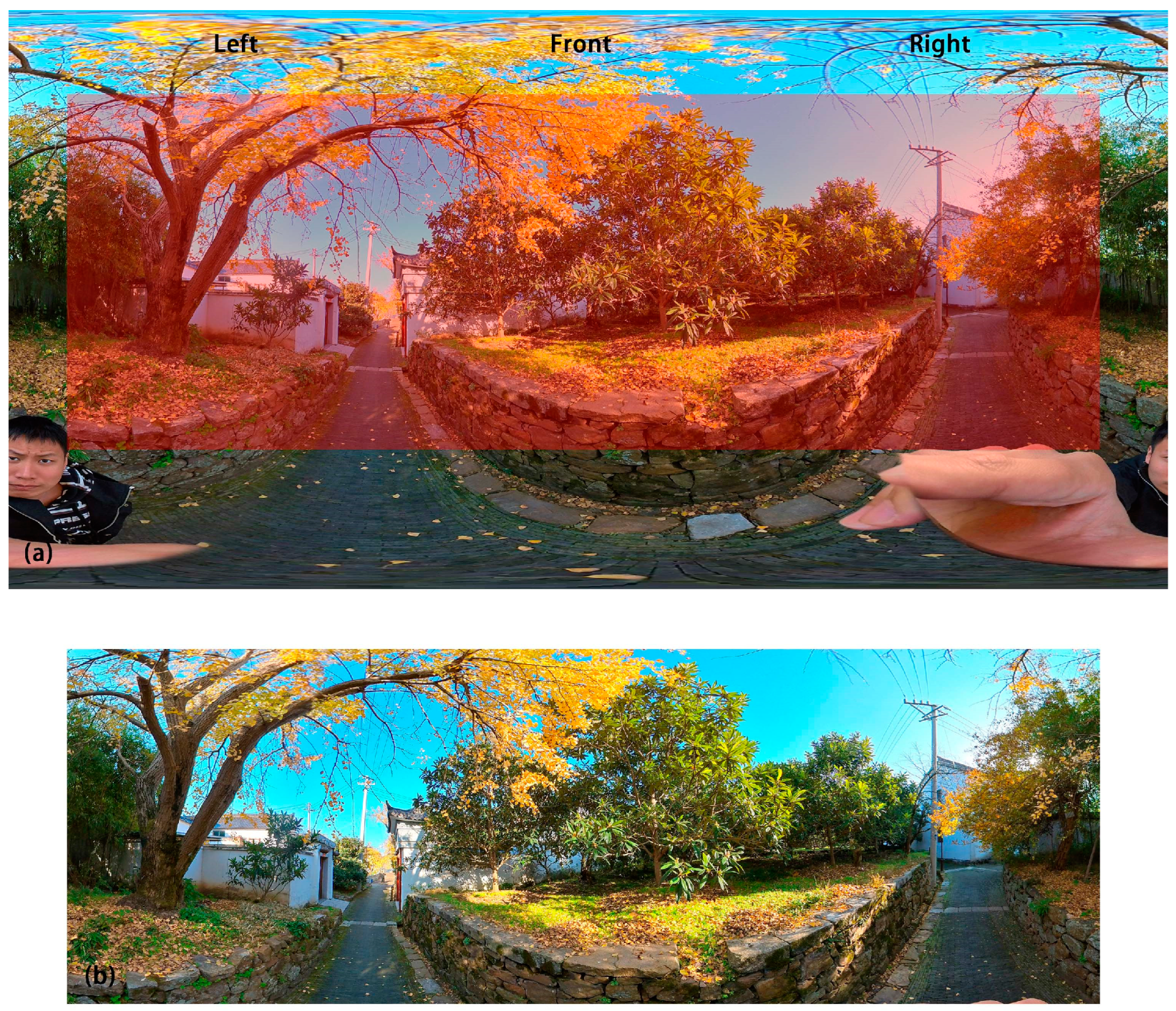It is widely applied in various types of landscapes, such as rural settlements, roads, waterfronts, settlements, national parks, and so on [19,44,45]. Taking into account time and economic costs, existing studies have mainly used landscape photographs as the evaluation medium, but the content of traditional photos was limited by the angle of view, making it difficult to show the panoramic view. Currently, judging the visual quality of landscapes based on the scenic beauty evaluation method mainly involves calculating the evaluator’s composite score for the scene’s environment, which is invariably limited by the sample data volume.

Based on the above analyses, landscape features in the three dimensions of landscape components, colors, and spatial forms of plant landscape all have an impact on public landscape aesthetic sensory perception. Existing studies mainly remain on the topic of qualitative description of landscape characteristics and explore the relationship between landscape characteristics and aesthetic preference from a single dimension, which often leads to a low prediction model of landscape aesthetic preference, and makes it difficult to effectively explain the main landscape feature indicators affecting aesthetic sensory perception.

To address these research gaps, this study aims to improve the accuracy of the landscape aesthetic sensory assessment methods from both the construction of the landscape characteristic index system and landscape preference judgment. First, based on the previous single dimension of spatial form features, landscape components and plant color features are added to expand the landscape special index system. A quantitative description of indicators is achieved with the help of digital technology. At the same time, the traditional beauty degree evaluation is improved, and the score of each evaluation subject for the scene environment is calculated, expanding the sample data volume. Finally, the relationship between multi-dimensional landscape characteristics and landscape aesthetic preference is constructed. It will provide a theoretical basis and references for the refined conservation and regeneration of the landscape of traditional villages.

2. Materials and Methods

2.1. Research Area

Dongshan and Xishan are located in the southwest of Suzhou, on the east bank of Taihu Basin, which is close to Shanghai. Suzhou is located in the southeast of Jiangsu Province, which belongs to the eastern coastal area of China. The region has a long history of congregation which can be traced back to the earliest Spring and Autumn Period in the Wuyue Kingdom. A dozen ancient villages are distributed in Dongshan and Xishan, and most of them lie in front of mountains and boast rivers around, showing distinguishing regional characteristics. Dongshan is a peninsula that extends into Taihu Lake, surrounded by water on three sides, with a total area of 96.6 square kilometers. The existing resident population of it is more than 5300. Xishan Island belongs to the islands in the lake, with an area of about 79.8 square kilometers, and the current population of it is about 45,000 people. Four representative traditional villages at national level with relatively well-preserved historical features, namely Yangwan Village, Wengxiang Village, Dongcun Village, and Zhili, were selected for this study. Yangwan has an area of about 11.86 square kilometers and a resident population of more than 3600; Wengxiang has an area of 3.77 square kilometers and a resident population of approximately 1000; Dongcun has an area of 0.07 square kilometers and a population of about 700; and Zhili covers an area of about 2.1 square kilometers and has a population of approximately 2000. The study selected 31 typical open outdoor spaces in villages where residents and visitors carry out daily communication, activities, and recreation based on field visits (Figure 1) [9], and the boundaries of the sample plots were limited to forest edges, road edges, or corner lines of building side walls.

2.2. Data Collection

To restore the true feelings of people in open space, this study was based on panoramic pictures to judge aesthetic preferences and to identify landscape elements and color features. Panoramic photographs were taken using a fixed standard of shooting to simulate the human point of view and comprehensively display the landscape features; the cameras were placed in the center of the scene at the height of 1.6 m; and the photographs were taken with the same Insta360 ONE X2, which was connected to the cell phone with the positioning enabled by Bluetooth. It helped to locate the geographic coordinates and the photographs were taken over 3 days from 23–25 November 2021, 9:30–11:30 a.m. and 2:00–4:00 p.m. During this period, the weather conditions were favorable and climatic conditions were similar.

A handheld 3D laser scanner, model GEOSLAM ZEB-HORIZON, collected spatial morphology data. The experimental staff member held the instrument in front of their chest, then started walking from the starting point around the field. Then, he returned to the origin to form a closed loop. Data collection was completed in this way. The spatial collection of morphology data was completed at the same time.

2.3. Research Methods

The research was structured into five steps. In the initial stage, a semantic segmentation model was employed to quantitatively identify visual attraction elements within traditional village public space landscapes, utilizing panoramic photos as the primary data source. Subsequently, in the second step, a combination of colorimetric and software methods was applied to extract the color information of plant communities through Colorimpact 4 software (Tiger Color, Akershus, Norway). The color characteristics were then quantitatively described based on the Munsell color card theory. Moving on to the third step, three-dimensional laser scanning technology was introduced. The irregular three-dimensional space of plant landscapes was characterized using the R language 4.1.0 (R Core Team, Vienna, Austria). The fourth step involved an enhancement of traditional beauty evaluation methods, integrating virtual reality technology to assess the aesthetic preferences of the landscape scenes. Lastly, predictive models for aesthetic sensory perception, tailored to different scenarios, were developed.

2.3.1. Identification of Visually Attractive Elements of the Landscape

• Image Pre-processing

With color panoramic photographs as a medium, we used the image analysis method during the research to evaluate the quality of rural plant landscapes. As a proxy for real-life scenes, pictures could effectively measure the psychological and aesthetic feedback of the visitors. In addition, with a wide field of view, panoramic images could comprehensively record the study site’s visual information and facilitate their quantitative analysis by computer vision techniques. About 28.8% of the periphery of the panoramic images had severe distortions. In contrast, the central portion of the camera lens with a vertical field of view spacing of ±30° had less distortion and better matched the visual range of human eyes [46,47]. We referred to the method of Li Yin and Zhenxin Wang to exclude the most distorted part of the image caused by the camera lens by cropping out part of the image. This method could retain the observation content closer to the human perspective [48]. The vision frame showed the view areas reflecting eyelevel equivalent pedestrian experience for three directions: front (A), left (B), and right (C) (e.g., Figure 2). Additionally, the content with the vision frame was low in degree of distortion.

2.

Scene elements identification and extraction

We used the deeplabv3 model trained on the ade20k dataset to extract the scene elements. Ade20k has strong generalization properties, and its extensive use in rural studies verifies its reliability for extracting elements of rural scenes [49]. In addition, the ade20k dataset can identify tree, grass, plant, and sky elements (

Table 1. Landscape element identification.

Index	Explanation
Percentage of structure (Structure)	Structure = (Swall + Sbuilding)/S. In the formula, Sstructure represents the pixel area of the structure, including walls and buildings; in the scene, S represents the total pixel area of the panoramic image.
Percentage of sky (Sky)	Sky = Ssky/S. In the formula, Ssky represents the pixel area of the sky; in the scene, S represents the total pixel area of the panoramic image.
Percentage of earth (Earth)	Earth = Searth/S. In the formula, Searth represents the pixel area of the earth; in the scene, S represents the total pixel area of the panoramic image.
Percentage of grass (Grass)	Grass = Sgrass/S. In the formula, Sgrass represents the pixel area of the grass; in the scene, S represents the total pixel area of the panoramic image.

), which meets the needs of this study. From the pre-experimental results, image segmentation trained by this dataset was more fine-grained and could accurately outline the countryside plants as well as other elements. As a result, we applied this method to extract each kind of element from all images (e.g., Figure 3).

2.3.2. Feature Identification of Landscape Colors

Color elements are quantitative indicators that condense most information in the color composition and the color space pattern. The usual means of recording color data in previous studies is to record the RGB values of colors [42]. But, the RGB triple values are in fact not regular. It is challenging to quantify colors from the perspective of the visual sensory characteristics of the human eye, making it difficult to apply the study’s results in practice. To solve the above problems, the HSV color model (Hue, Hue, H; Saturation, Saturation, S; Brightness, Value, V) is suitable for the visual characteristics of the human eye. This model was chosen to divide the color threshold interval, which was the one that most closely matched the human eye’s ability to perceive colors and can quantify colors non-isotropically and uniformly from the perspective of the human eye’s sensory perception of the color characteristics. In conducting this study, the researcher used the ColorImpact 4 software (Tiger Color, Akershus, Norway) to extract the colors present in plant elements. Following this, researchers utilized the quantification method to categorize the non-uniform colors in the HSB color model into intervals of H (Hue): S (Saturation): V (Brightness) = 8:4:4. This process successfully yielded a total of 128 distinct colors (e.g., Figure 4). Representative colors in the same interval range were used to divide the color intervals, which was convenient for quantifying and analyzing the color data in the later stage. The HSV color model was used to describe the detailed color characteristics of plants. According to the non-uniformly quantified color intervals, the colors were divided into different interval ranges, and the three color components were evaluated in a one-dimensional feature vector, that is, L = H × G s × G v + S × G v +V. In the formula, H, S, and V denote the hue, saturation, and luminance, respectively; Gs and Gv denote the number of quantization levels for S and V, which both have 4 levels. Therefore, the final expression was L = 16 H +4 S + V. It could be seen that the weight distribution of the hue is the largest. So, hue was the main factor to distinguish the color characteristics. The related derived indicators were calculated based on the three HSV indicators (e.g.,

Table 2. Landscape color recognition.

Index	Explanation
Number of Colors (NC)	NC = SUM(HaSbVc); HaSbVc ≥ 1%. NC represents the total number of extracted colors, excluding black, white, and gray, with a pixel percentage of more than 1%.
Main Hue Comparison (MHi)	MHi = NMHi/N × 100. NMHiis the pixel of primary color which occupies the largest pixel area in the scene; N is the total number of pixels of the image.
Adjacent Hue Comparison (NHi)	NHi = NHi/N × 100. NHi is the pixel of adjacent colors which are within 60 degrees of each other on the left and right of the primary color in the hue circle; N is the total number of pixels of the image.
Complementary Hue Comparison (CHi)	CHi = NCH/N × 100. NCH is the pixel of complementary colors which are within 180 degrees of the primary color; N is the total number of pixels in the image N is the total number of pixels of the image.
Warm and cool color tone contrast (THi)	THi = NHf/NHw × 100. NHf is the pixel of cool colors; NHw is the pixel of warm colors.
Color Diversity Index (H’)	$\mathrm{H}’={\displaystyle \sum }_{\mathrm{i}=1}^{\mathrm{S}}\mathrm{Pi}\ln \mathrm{Pi}$; Pi represents the percentage of color i; S represents the total number of extracted colors, S = NC.
Color Evenness Index (E’)	E’ = H’/lnS. H represents the color diversity index; S represents the total number of extracted colors, S = NC.

) [50].

2.3.3. Identification of the Spatial Morphology Characterization of the Landscape

• Data pre-processing

Firstly, the point cloud data were cropped, denoised, and ground points were extracted and normalized to retain the relevant point clouds in the study area while reducing the amount of data. Then, cropped and retained the necessary study objects and separated the hard surfacing point cloud and the tree canopy point cloud for subsequent analyses. Due to the influence of external factors such as human beings or animals, many outliers, namely noisy points, inevitably existed in the point cloud data. To improve the accuracy of subsequent data analysis, noise reduction processing was required. In this study, the distance between points was applied as the primary measure. On the basis of the experience of previous experiments, it was set to be 10 points in surroundings. Then, the median and standard deviation of the average distance of the points in the domain were calculated. Meanwhile, to improve computational efficiency, the box grid filer was set to 0.1 m for filtering based on satisfying the computational accuracy, and the sample point cloud was reduced from ten million orders of magnitude to less than 50 w.

2.

Construction of spatial morphology characterization indexes

This study utilized a traditional index system to characterize the spatial morphology of public areas in the village that have been previously constructed. The system is based on three-dimensions horizontal interface, vertical interface, and three-dimensional spatial level. It included various parameters such as accessible area ratio (AAR), eccentricity rate (E), Spatial Shape Index (SSI), Average Height of Upper Contour (hu), average height of lower contour (hl), solid-space ratio (SVR), contour fluctuation range (FR), fluctuation variance of upper contour (FVU), fluctuation variance of lower contour (FVL), vegetation coverage (VC), plant diversity index (PDI), three-dimensional green visibility (3D-GVI), enclosure degree (ED), and composite closure (CC) [9]. These 14 spatial morphology indicators were used.

3.

Quantitative identification of spatial morphological indicators

Indicators were mainly calculated using Lidar360 v3.2 software combined with R language. The area and length class indicators were calculated by projecting the point cloud of the study area to the XOY plane, and then carrying out edge extraction to identify the edge contour, thus calculating the area within the contour. The height metrics were calculated by outputting the point cloud data as raster data, thus calculating the edge height within the raster. The long and short axes in the site were calculated using the traversal method, which calculated the Euclidean distance from each point to each of the other points, with the maximum value being the long axis and the minimum value being the short axis. The 3D canopy volume was calculated using the α-shape method to construct convex packets and accumulate the volume of each convex packet to derive the 3D green volume.

2.3.4. Evaluation of Landscape Aesthetic Preference

This research has been approved by the Ethics Review Board of Nanjing Forestry University and the participants have given their informed consent. Scenic beauty estimation (SBE) is widely used to evaluate landscape quality, focusing on visitors’ aesthetic feelings for landscape scenes. Considering the evaluator’s ability to operate technological products and excluding the influence of utilitarian aesthetics, this study selected a total of 64 students and experts with landscape professional backgrounds, of which 40 were students, and 24 were experts, for scoring. The panorama photos were imported into the Baidu VR platform, and the images were converted to human perspective 360° autonomous rotating VR images, and the evaluators wore VR glasses with the VIVE-VR model for evaluation and scoring. The evaluation rating was divided into 5 levels, with corresponding scores from 1 to 5, indicating dislike very much, dislike, neutral, like, and like very much, respectively. The value of SBE was calculated based on scoring from multi-population for the scenes. In this study, the quality of the 31 rural landscape scenes was audited directly by the results of visitor scoring. As each visitor could be taken into account, compared to calculating the SBE, the method in this study effectively expands the sample size (64 times the SBE).

The validity of visitor scoring has been proved in previous studies related to SBE. This study used one-way ANOVA to test whether there is a difference in the scoring of different scenes. On this basis, this study used the ICC (intraclass correlation coefficient) to evaluate the reliability scale between expert and student scoring on the same scene.

2.3.5. Statistics Analysis

• Data pre-processing

The three types of indicators of the rural plant scene differ greatly in their scale due to their different sources as well as units of measurement. Therefore, they were subjected to maximum–minimum normalization to map the data features into the interval [0, 1] and remove the influence of the scale on the assessment results. The formula is as follows:

$$X_{mmx}=\frac{X-X_{min}}{X_{max}-X_{min}}$$

where $X$ is the original data, $X_{mmx}$ is the normalized data, and $X_{min}$ and $X_{max}$ are the minimum and maximum values of the original data, respectively.

2.

Assessment Model Establishment

In previous studies, the excellent assessment capability of a linear model for SBE grade evaluation was validated. This study utilized a multiple linear regression model to predict visitor scoring by selecting indicators such as spatial morphological characteristics, feature composition, and vegetation color characteristics of rural plant scenes as predictors. The parameters of the linear model were solved using the least squares method. The model formula is as follows:

$$\widehat{Y}={\beta }_1{X}_1+{\beta }_2{X}_2+\dots +{\beta }_n{X}_n+{\beta }_0$$

where $\widehat{Y}$ is the assessment of visitor scoring, $n$ is the number of predictors included in the model, $X_n$ is the $n$th predictor, and ${\beta }_n$ is the standardized regression coefficient of the $n$th predictor.

In addition to the full model with all indicators as predictors, the optimized model with streamlined indicators as predictors was established. Based on principal component analysis, indicators with a higher contribution rate were selected for all-subsets regression analysis. Adjusted R², Mallows’ Cp (Cp), and the Bayesian Information Criterion (BIC) were used to determine the optimized model.

3. Results

3.1. Result of Public Landscape Preference

Figure 5 illustrates the results of the scores from 40 students and 24 experts. The one-way ANOVA result (F = 147.005, Sig < 0.001) indicated that the difference in scoring across 31 scenes was statistically significant, while the ICC result (ICC = 0.969, p = 0.00107) indicated the agreement between experts and students in scoring. In other words, the difference in visitors’ aesthetic feelings for 31 scenes, and these differences were not affected by visitors’ professional background. Accordingly, this study treated experts’ and students’ scoring of scenarios consistently.

3.2. Quantitative Recognition Results of Landscape Features

3.2.1. Quantitative Results of Spatial Morphology

The quantitative result of spatial morphology is shown in

Table 3. Results of morphological quantification.

Spatial Composition	Morphological Characteristics Index	Minimum	Maximum	Mean Value	Standard Deviation
Horizontal interface	AAR	0.076	0.8563	0.3145	0.1819
	E	0.1455	2.7862	1.4489	0.5351
	SSI	29,816.11	1,381,168.18	257,269.50	302,740.87
	VC	0.2014	0.9202	0.6102	0.3519
Vertical interface	SVR	0.0015	0.0174,	0.0056	0.0033
	FR	0.4146	1.9128	0.9397	0.3339
	hu	4.2324	27.5353	11.9914	5.3382
	hl	0.4996	5.3626	2.2667	1.1749
Three-dimensional space	3D-GVA	0.0397	0.2608	0.1094	0.0548
	ED	0.0037	0.2161	0.0731	0.0484
	CC	0.0753	0.5337	0.2365	0.1301
	PDI	0.1732	1.8919	1.105	0.4049

. The value of the variance of the upper and lower contour fluctuations was in the range of 10–16 levels, indicating that the drastic degree of upper and lower contour fluctuations of traditional villages in the Dongshan and Xishan regions was extremely small. So, the data in the table were not shown. The average of the accessible area ratio (AAR) value of the sample plots in the horizontal interface indicator (HII) reached 31.45%, and the average value of the eccentricity of bottom surface morphology (E) of the sample plots was 1.4489. Most of the sample plots showed a narrow and elongated morphology. The average spatial shape index (SSI) value was 257,269.50, and the standard deviation reached 302,740.87, indicating that the bottom surface morphology of the sample plots was more complex. The vegetation coverage (VC) of the sample plots was generally high, with a mean value of 60%. The average height of the upper layer of vegetation (hu) ranged from 4.23 m to 27.54 m. The average height of the lower layer of vegetation (hl) ranged from 0.50 m to 5.36 m, which indicated that the vegetation in the villages was generally higher, and the lower layer of shrubs was lower. The solid-to-void ratio (SVR) of vertical interface ranges from 0.0015 to 0.0174, with a mean value of 0.0056, indicating that the vertical interface was more open. The three-dimensional morphology index enclosure (ED) indicator ranged from 0.0037–0.2161 with a mean value of 0.0731, and the composite closure (CC) ranged from 0.0753–0.5337 with a mean value of 0.2365, with both indicators indicating high spatial openness. The three-dimensional spatial green visibility (3D-GVA) ranged from 0.0397 to 0.2608, with a mean value of 0.1094. Meanwhile, the plant diversity index revealed that the selection of tree species in villages was relatively unified.

3.2.2. Results of Landscape Element Identification

The results of the identification of landscape elements are shown in

Table 4. Results of landscape element identification.

Landscape Elements	Minimum	Maximum	Mean Value	Standard Deviation
structure	0.0084	0.5693	0.3114	0.1987
sky	0.0236	0.4923	0.2892	0.1205
earth	0	0.1881	0.0539	0.0556
tree	0.0155	0.4382	0.1448	0.1035
grass	0	0.1488	0.0194	0.0398

below. Vegetation and structure were the leading landscape elements that constituted the open space of traditional villages. The structure proportion ranged from 0.84% to 56.93%, with a mean value of 31.14% and a standard deviation of 0.1147. The proportion of bare land in the sample space was low, and the mean value was 5.39%, which indicates that the open space of traditional villages in the region had a high green coverage rate, except for hard paving. The mean value of the proportion of trees in the scene environment reached 14.48%, and the interval range was 1.55%–43.82%, while the proportion of the lower ground cover was lower, with a mean value of 1.94%. The data indicated that the vegetation level in the sample space is more homogeneous, with fewer shrubs in the middle layer.

3.2.3. Results of Landscape Color Recognition

The results of the identification of scene landscape color features are shown in

Table 5. Results of landscape color recognition.

Landscape Color Characteristic Index	Minimum	Maximum	Mean Value	Standard Deviation
Number of Colors (NC)	3	8	5	1
Main Hue Comparison (MHi)	0.0057	0.2252	0.0853	5.6911
Adjacent Hue Comparison (NHi)	0.0022	0.1712	0.0496	4.3807
Complementary Hue Comparison (CHi)	0	0.0024	0.0041	0.582
Warm and cool color tone contrast (THi)	0	0.6223	0.0757	0.1256
Color Diversity Index (H’)	0.0444	0.884	0.4244	0.2119
Color Evenness Index (E’)	0.0404	0.5493	0.2456	0.121

below. The number of colors ranged between 3–8, with an average of 5 colors per scene. The main hue of the scene environment was reddish, with low saturation and low value. The distribution of hues in the scene was more dispersed, with fewer neighboring colors, the range of the main hue was 0.57%–22.52%, and the proportion of neighboring colors was 0.22%–17.12%. The scene had almost no complementary colors, and the proportion of complementary colors tended to be 0. The scene environment mainly showed warm tones, and the proportion of warm and cold colors ranged from 0 to 62.23%. The mean value of the color diversity index reached 0.42, with a wide range of colors. However, the color index was not high, with a mean value of 0.25 and a range of 0.04–0.55.

3.3. Landscape Preference Assessment

3.3.1. Indicator Screening

To reduce the parameters and dimensions of the calculation, this study conducted a principal component analysis of the indicators. It calculated the contribution of each indicator in different principal components. Significantly, the first seven principal components and the second principal component presented more than 75% of the information (

Table 6. Total variance explained.

Component	Initial Eigenvalues			Extraction Sums of Squared Loadings
	Total	% of Variance	Cumulative %	Total	% of Variance	Cumulative %
1	5.843	22.475	22.475	5.843	22.475	22.475
2	3.774	14.515	36.99	3.774	14.515	36.99
3	3.335	12.826	49.815	3.335	12.826	49.815
4	2.452	9.429	59.244	2.452	9.429	59.244
5	1.96	7.539	66.783	1.96	7.539	66.783
6	1.755	6.749	73.532	1.755	6.749	73.532
7	1.373	5.281	78.813	1.373	5.281	78.813
8	1.22	4.692	83.505	1.22	4.692	83.505

) [9]. Therefore, we only took the index contribution rates in the first seven principal components into consideration. Descriptions of the contribution rate of each indicator are in the figure below (Figure 6). Indicators that contributed more than 50% were screened: AAR, VC, FR, hu, hl, FVu, 3D-GVA, CC, structure, tree, MHi, Nhi, CHi, THi, H’, and C’.

The 16 screened indicators were adopted in the all-subsets regression (Figure 7). When the predictors were seven, adjusted R² peaks, and Cp and BIC were minimized, indicating that the model with streamlined indicators was optimal, and the corresponding predictors were AAR, FR, CC, tree, NHi, CHi, and THi.

3.3.2. Result of Public Landscape Preference Assessment

All indicators as predictors were included in the multiple linear regression to build Model 1; the streamlined 7 predictors were included in the multiple linear regression model to build Model 2. As shown in

Table 7. Model summary.

Model	R	R2	Adjusted R2	Std. Error of the Estimate	Durbin-Watson
1	0.813	0.661	0.656	0.812	0.586
2	0.702	0.493	0.491	0.988	0.389

, the adjusted R² = 0.656 for Model 1 indicated that all indicators explain 65.6% of the variation in visitor scoring. The adjusted R² = 0.491 for Model 2 indicated that the 8 streamlined indicators explain 49.1% of the variation in the visitor scoring. The Durbin–Watson values for Model 1 and Model 2 were 0.586 and 0.389, respectively, and were both consistent with independence. The two models’ residual histograms and P-P plots were as follows (Figure 8 and Figure 9). The residual histograms obeyed the normal distribution, the mean was close to 0, and the standard deviation was close to 1 (standard normal distribution), which meant that the linear regression was attained at the condition of normality. At the same time, the P–P plots also indicated that the model matches the condition of normality, which thoroughly explained the validity of the models.

Table 8. Model coefficients.

Model	Predictors	B	β	t	p
1	(Constant)	0.362		0.416	0.678
	AAR	2.657	0.44	11.531	0
	E	−1.93	−0.278	−10.088	0
	SSI	0.738	0.117	2.475	0.013
	VC	0.766	0.142	1.846	0.065
	SVR	5.005	0.735	15.308	0
	FR	1.774	0.281	2.428	0.015
	hu	−3.222	−0.524	−4.124	0
	hl	2.827	0.485	10.427	0
	FVu	−0.531	−0.072	−1.837	0.066
	FVl	2.245	0.298	7.731	0
	3D-GVA	−2.106	−0.371	−9.438	0
	DOE	−0.942	−0.152	−2.417	0.016
	CC	−1.312	−0.265	−4.416	0
	PDI	−1.859	−0.283	−9.696	0
	Structure	0.181	0.046	0.918	0.359
	Sky	1.41	0.247	4.347	0
	Earth	−1.108	−0.233	−7.882	0
	Tree	2.081	0.364	4.209	0
	Grass	0.341	0.065	0.696	0.486
	NC	0.662	0.063	0.676	0.499
	MHi	1.258	0.232	3.531	0
	NHi	−0.735	−0.135	−1.559	0.119
	CHi	−3.13	−0.551	−15.23	0
	THi	1.978	0.343	5.849	0
	H’	−6.68	−1.198	−1.863	0.063
	C’	8.66	1.464	2.811	0.005
2	(Constant)	1.545		24.825	0
	AAR	2.801	0.464	21.084	0
	FR	2.433	0.385	17.638	0
	CC	−4.062	−0.819	−29.062	0
	Tree	1.811	0.317	11.063	0
	NHi	2.173	0.4	15.429	0
	CHi	−2.578	−0.454	−21.334	0
	THi	3.451	0.598	31.891	0

shows the coefficients for Model 1 and Model 2. VC, FVu, structure, grass, NC, Nhi, and H’ in Model 1 were not significant at 95% confidence intervals. This indicated that VC, FVu, structure, grass, NC, Nhi, and H’ hardly predict visitor scoring. Based on the beta coefficients, the accessible area ratio (AAR), spatial shape index (SSi), solid vacancy ratio (SVR), contour fluctuation variance (FVl), sky, tree, main hue percentage (MHi), warm and cool color tone contrast (THi), and color index (C’) can be entered into the Model 1 had a positive effect on landscape aesthetic preferences. Eccentricity (E), upper contour mean height (hu), three-dimensional green volume (3D-GVA), degree of enclosure (DOE), composite closure (CC), plant diversity index (PDI), earth, and complementary color ratio (CHi) had adverse effects on landscape aesthetic preferences. The final model expression for Model 2 was:

$$\widehat{Y}=0.464\mathrm{AAR} +0.385\mathrm{FR}-0.819\mathrm{CC}+0.317\mathrm{TREE}+0.4\mathrm{NHi}-0.454\mathrm{CHi}-0.598\mathrm{THi}+1.545$$

4. Discussion

To advance the regional and cultural significance of landscape resources in urban-rural areas and promote the sustainable development of villages, tourism, and cultural exchanges, we needed to understand the connection between aesthetic sensory perception and the landscape environment and identify which landscape characteristics could contribute to human mental and physical status and well-being. Many studies have explored landscape characteristics and public aesthetic preferences from a single dimension. However, studies integrating multidimensional features to explore the factors that influence landscape preferences were still scarce. There were many limitations, such as insufficient quantification of landscape feature indicators and low accuracy of landscape preference assessment models. This study aimed to compensate for these deficiencies in two aspects. First, based on the existing landscape spatial morphology dimensions, this study expanded the landscape feature characterization system by introducing two dimensions, namely, landscape visual attraction elements and plant landscape color. At the same time, the traditional beauty degree evaluation was improved and the score of each evaluation subject for the scene environment was calculated, expanding the sample data volume. We focus on two main research questions: (1) identifying the main features that influence landscape aesthetic preference and analyzing the influencing mechanisms; (2) how to improve the progress of the landscape aesthetic preference assessment model. The following discussion will focus on these two aspects.

4.1. Expanding the Dimensions of Landscape Characteristics Influencing Aesthetic Sensory Perception

The results of the study showed that seven landscape feature indicators, namely, accessible area ratio (AAR), fluctuating range of contour (FR), comprehensive closure (CC), tree, neighboring color ratio (NHi), complementary color ratio (CHi) and warm and cool color tone contrast (THi), had a significant effect on aesthetic preference. The influence of trees on landscape preference at the level of landscape elements was significantly higher than that of other elements, and it was a positive factor that affected aesthetic sensory perception. Trees were the primary type of vegetation in the public space of traditional villages, and in line with previous studies, an aesthetically pleasing environment was associated with plants [51,52,53]. The positive influence of plants, as the leading natural element of landscape composition, could be explained by ecological and evolutionary theories. They could create an environment where the provision of nature allowed for humans to retain an affinity for the original natural ecological dynamics and humans could enjoy the natural environment and the relaxing atmosphere [54]. The previous study’s explanation for the Chinese people’s fondness for village plants was that urbanization in China over the past few decades had caused severe ecological damage and that economic development had intensified the demand for green space, thus making lush vegetation the ideal image of the village landscape for tourists [54]. The type of village vegetation (herbaceous vs. tree) in the study by Arriaza et al. did not produce a statistically significant effect in the regression analysis of the variables, while the percentage of vegetation in the picture was considered an important attribute of the village landscape [20]. Whereas the vegetation cover type trees had a statistically significant effect in this study, herbaceous trees did not provide an adequate explanation for the public aesthetic preference, which may be related to the monoculture vegetation composition of traditional villages because the percentage of herbaceous was relatively low there and was dominated by tall trees and crops, excluding the bare land.

Accessible area ratio (AAR) and contour fluctuation range (FR) in the spatial form dimension were positive factors that significantly affect landscape aesthetic preference. Comprehensive closure (CC) negatively affected landscape aesthetic sensory perception. Accessible area ratio (AAR) somehow indicates the space available to the public per unit of area. The description of popular landscape scene environments in previous studies was large landscape spaces that were naturally open and suitable for transportation and activities, giving a sense of nature [55,56]. It suggested that the accessibility of landscape spaces and the social and recreational activities that they accommodated had a positive effect on landscape preferences. This was consistent with landscape sensory restoration theory, where one of the four characteristics of restorative environments was compatibility. It suggested that good landscape spaces had sufficient content and structure to provide activities that were relatively consistent with individual purposes and preferences, thus satisfying the activity needs of different users [57]. Previous studies have shown that people preferred scenic environments that were open in scale and organized, which was different from the results of this study [58,59]. The contour fluctuation range (FR) indicated the size of the fluctuation range of the highest point of the plant canopy line at the vertical interface, which to some extent destroyed the orderliness of the vertical interface. The study by Zhang et al. showed that the interactions between visual attributes could lead to inconsistencies in the interpretation of the main influences on landscape preference [39]. After careful analysis, it was be found that the range of contour fluctuation (FR) and the variance of upper contour fluctuation (FVu) together reflected the orderliness of the contour on the vertical interface. In this study, the upper contour fluctuation variance (FVu) was infinitely close to 0, which indicated that the intensity of contour fluctuation on the vertical interface in the 31 scene environments was very small. It had already possessed good order in itself, while the increase in the fluctuation range was to strengthen the richness of the whole map surface. Thus, the landscape preference of the scene was enhanced, which validated previous research that richness showed an unstable effect on people’s preference, and that richness had a positive effect only if the sense of order was high [60]. Berlyne’s study also explained this phenomenon by suggesting that there was an inverted U-shaped functional relationship between scene richness and landscape preference, where landscape preference was initially positively related to scene richness, and then negatively related when a certain threshold was reached [61]. The composite closeness index (CC) measured the degree of closeness of the whole scene environment. It was negatively correlated with landscape aesthetic preference but in line with the explanation of people’s preference for scenes with open visual scales in previous studies, while it seemed to contradict the explanation of people’s preference for scenes with a high proportion of tree elements. Prospect-refuge theory can provide a reasonable explanation for this: people want to be able to observe others but not be seen by others [62]. The openness of the line of sight provides a good viewing experience, and the increase in the proportion of trees enriches the depth of the field of view, while providing a certain degree of shading.

The proportion of neighboring hues (NHi) and the proportion of warm and cool hues (THi) at the dimension of landscape color characteristics were positively correlated with landscape perceptual preference, and the proportion of complementary hues (CHi) was negatively correlated with it. Previous related studies have shown that large areas of warm-colored plants in autumn can create a warm and peaceful feeling, and the combination of adjacent red and yellow colors makes it more likely to form a harmonious color combination [63]. With a softer and more fluid excess between colors, it helps the public to process visual information more easily, and at the same time creates an emotional experience of calmness, gentleness, and serenity, which is thus preferred by the public [64]. These results explained the positive effect of the proportion of neighboring hues (NHi) on landscape preference in this study, where panoramas were also collected in autumn, and the color of the foliage trees were dominated by reddish-yellow tones. Zhuang et al. showed that increasing the proportion of cool colors and green vegetation in the urban floristic mirror can enhance aesthetic preference [40], which was in line with the results of the present study but contrary to the findings of Luo et al., which were consistent with the results of this study but contrary to the results of Luo et al. A possible explanation for this was that based on the theory of color psychology, warm colors are more likely to produce physiological stimulation than cool colors, and rural landscapes are considered to be rejuvenating or tranquil environments [51,65,66]. The proportion of cool-colored vegetation in the 31 scenes was generally small. Scenes in which the proportion of cool-colored evergreens was slightly higher were more likely to create an atmosphere of calmness, gentleness, and serenity, thus enhancing people’s aesthetic preference. Luo et al. showed that the number of experimental colors is between 5 and 7. Among them the color leaf index was high, and the large area of uniform fall warm colors were easily preferred by the public [64]. This can be used to explain why the complementary hue ratio (CHi) hurt landscape aesthetic sensory perception in this study. The sample sites selected in this study had relatively few plant species, of which were colorful foliage plants of similar hues. And the whole picture was relatively uniform, so the increase in complementary colors would destroy the sense of order of the whole picture and make it difficult to obtain uniformity. The study by Kuper showed that attentional restoration was positively correlated with landscape sensory perception, and according to the theory of attentional restoration, exposure to warmer colors was more likely to be preferred by the public [67]. According to the theory of attention restoration, exposure to restorative environments will cause fascination or effortless attention, which can also explain people’s preference for scene environments with low complementary hue ratios and relatively uniform hues.

Based on the above analysis, we can describe the ideal public space scene environment of traditional villages, where people can enjoy a wide view, a high proportion of trees, and mild and uniform color tones. The ideal public space is suitable for passages and activities and can produce a restorative and peaceful atmosphere. The way people pay attention to the landscape and the attractiveness of landscape features differs in different landscape sensory perceptions, and landscape features are directly affected by the sensory process, so these sensory perceptions can be strengthened by artificial landscape feature design. Although landscape preference is influenced by many aspects, the most important factor affecting the landscape preference of traditional villages is related to the ideal image of the countryside in people’s minds, which is based on the symbolic experience of the perceiving subject for the space. In the subsequent renewal and protection of traditional villages, government authorities and planning and design departments should encourage public participation, considering the physical structure of the landscape in conjunction with its value and meaning, to create a more inclusive environment, thus promoting the sustainable development of rural habitat.

4.2. Improvement of the Effectiveness of the Aesthetic Sensory Assessment

Compared with previous studies, this study mainly improved the accuracy of model assessment accuracy from in various aspects. On the one hand, we analyzed the previous landscape scores and the scores of each evaluation subject separately. The sample number was expanded to 64 times of that of the original, which helped to obtain more stable assessment results. On the other hand, based on the previous spatial morphology single-dimension indicators, two-dimensional feature indicators of landscape visual elements and landscape color were introduced, which helped refine the influence dimensions of aesthetic sensory perception. The conditions were conducive to a more comprehensive understanding of the landscape characteristics of the public space of traditional villages. Previous studies have shown that the multiple linear regression model was more advantageous in the assessment of landscape rating, with the coefficient of determination R² = 33.2% and root mean square error RMS = 64.774, but only four significantly related morphology index factors were selected to participate in the construction of the model, making it difficult to understand the influence of other index factors on the assessment of landscape preference. In this study, the multiple linear regression model was also chosen to predict landscape preference, and all indicators of the three dimensions were included in the construction of the model, with the adjusted R² reaching 65.6%. The study streamlined the indicators based on the comprehensive indicator multiple linear regression model, screening seven significantly related indicators through principal component analysis and full subset regression analysis to participate in the model construction, and the R² of the streamlined model reached 49.1%, which was also higher than that of 33.2% in the previous study. Both models demonstrated the scientific rationality of the increase in indicator dimensions, and the assessment accuracy of landscape preference was effectively improved based on the previous single dimension. At the same time, the two models could be adapted to different scenarios. The full-indicator assessment model contains all the available indicators, comprehensively considers the landscape characteristics, and better captures the diversity and comprehensiveness. They paid attention to the interrelationships between the indicators of different dimensions, which contributed to the fine management and enhancement of the landscape of the public space of traditional villages. The streamlined predictive model was suitable for rapid judgment of environmental aesthetic sensory perception and could quickly improve the quality of spatial landscape environment in a short period.

4.3. Limitations and Future Work

Aesthetic sensory perception is a multidimensional perception process, which is jointly influenced by the aesthetic object and the perception subject. Although this study added two dimensions of landscape visual attraction elements and landscape color characteristics based on previous studies, the influence of other dimensions of landscape characteristics cannot be excluded. Subsequent studies should further improve the indicator system of landscape features and explore how the mutual combinations of visual attributes affect aesthetic sensory perception, as well as how to better control confounding factors to facilitate inter-comparisons between studies. Moreover, the morphological and color characteristics of plant landscapes are time-sequential. The landscape characteristics show great differences in different seasons or different periods of the same season. Therefore, subsequent research should further strengthen the identification of landscape characteristics at different times. At the same time, in the study, buildings, walls, and some other artificial facilities, including poles, were uniformly classified into structures without making further distinctions. Follow-up research will subdivide the composition of the structure and explore the impact of various visual attraction elements on aesthetic sensory perception. Although visual sensory perception is the main way of landscape aesthetics, the role of auditory, tactile, olfactory, and gustatory senses in the process of aesthetic sensory perception should not be ignored [68,69]. As a result, subsequent research should comprehensively consider the influence of human perceptual organs on aesthetic sensory perception. In addition, this study was based on the construction of aesthetic sensory perception assessment model for 31 scenarios of traditional villages in Dongshan and Xishan of Taihu Lake, Suzhou, and the values of each index have a certain range. Therefore, it is difficult to explore the relationship between landscape features and landscape preference beyond the range of the values, and the subsequent study needs to further increase the sample capacity to reveal the general pattern of the public’s aesthetic preference for the landscapes of the traditional villages. The following research needs to further increase the sample volume to reveal the general public aesthetic sensory perception of traditional village landscape.

5. Conclusions

This study expanded the landscape characterization system for the public space of the traditional village by integrating multiple dimensions: landscape spatial form, visually attractive elements of the landscape, and their colors. It quantitatively identified each index feature based on machine learning and LiDAR scanning technology. The traditional scenic beauty evaluation (SBE) method was improved to construct the aesthetic sensory perception assessment model with all indicators and indicators of significant influence. The accuracy of the full-indicator aesthetic sensory assessment model (R² = 65.6%) is higher than that of the significant influence indicator aesthetic sensory assessment model (49.1%). The assessment accuracy of both models is greatly improved compared with that of the assessment model of the previous study (R² = 33.2%). The results showed that the accessibility area ratio (AAR), spatial shape index (SSI), $\mathrm{solid} \mathrm{vacancy} \mathrm{ratio}$ (SVR), contour fluctuation range (FR), the average height of lower contour (hl), variance of lower contour fluctuation (FVl), sky, tree, main color hue (MHI), warm/cold hue (THi), and color index (C’) were able to enhance the public’s preference for public space in traditional villages. Eccentricity (E), average height of upper contour (hu), three-dimensional green volume (3D-GVA), degree of enclosure (DOE), comprehensive closure (CC), plant diversity index (PDI), earth, and complementary colors (CHi) reduced the public’s aesthetic preferences for the public space in traditional villages. Among them, the significant impact factors were AAR, FR, CC, tree, NHi, Chi, and THi. The study revealed the public aesthetic sensory perception of the public space of traditional villages, providing scientific and theoretical guidance and a basis for relevant decision-making departments and planning and design companies. Thus, it promoted the sustainable development of the rural living environment and provided a good relaxation environment for the physical and mental health of urban and rural residents.

References

1. Gao, J.; Wu, B. Revitalizing Traditional Villages through Rural Tourism: A Case Study of Yuanjia Village, Shaanxi Province, China. Tour. Manag. 2017, 63, 223–233. [Google Scholar] [CrossRef]
2. Grêt-Regamey, A.; Altwegg, J.; Sirén, E.A.; Van Strien, M.J.; Weibel, B. Integrating Ecosystem Services into Spatial Planning—A Spatial Decision Support Tool. Landsc. Urban Plan. 2017, 165, 206–219. [Google Scholar] [CrossRef]
3. Gebre, T.; Gebremedhin, B. The Mutual Benefits of Promoting Rural-Urban Interdependence through Linked Ecosystem Services. Glob. Ecol. Conserv. 2019, 20, e00707. [Google Scholar] [CrossRef]
4. Van Zanten, B.T.; Verburg, P.H.; Scholte, S.S.K.; Tieskens, K.F. Using Choice Modeling to Map Aesthetic Values at a Landscape Scale: Lessons from a Dutch Case Study. Ecol. Econ. 2016, 130, 221–231. [Google Scholar] [CrossRef]
5. Tveit, M.S. Indicators of Visual Scale as Predictors of Landscape Preference; a Comparison between Groups. J. Environ. Manag. 2009, 90, 2882–2888. [Google Scholar] [CrossRef] [PubMed]
6. Almeida, M.; Loupa-Ramos, I.; Menezes, H.; Carvalho-Ribeiro, S.; Guiomar, N.; Pinto-Correia, T. Urban Population Looking for Rural Landscapes: Different Appreciation Patterns Identified in Southern Europe. Land Use Policy 2016, 53, 44–55. [Google Scholar] [CrossRef]
7. Ecological Landscape Resource Management and Sustainable Development of Traditional Villages-All Databases. Available online: https://webofscience.clarivate.cn/wos/alldb/full-record/WOS:000588763500039 (accessed on 31 December 2023).
8. Park, J.J.; Selman, P. Attitudes Toward Rural Landscape Change in England. Environ. Behav. 2011, 43, 182–206. [Google Scholar] [CrossRef]
9. Chen, G.; Sun, X.; Yu, W.; Wang, H. Analysis Model of the Relationship between Public Spatial Forms in Traditional Villages and Scenic Beauty Preference Based on LiDAR Point Cloud Data. Land 2022, 11, 1133. [Google Scholar] [CrossRef]
10. Qi, L.; Liang, W.; Xi, M. The Public Space Pattern Research of Guangfu Traditional Villages Based on Spatial Syntax: A Case Study of Huangpu Village in Guangzhou City, China. IOP Conf. Ser. Earth Environ. Sci. 2019, 267, 062033. [Google Scholar] [CrossRef]
11. Déjeant-Pons, M. The European Landscape Convention. Landsc. Res. 2006, 31, 363–384. [Google Scholar] [CrossRef]
12. de la O Cabrera, M.R.; Marine, N.; Escudero, D. Spatialities of Cultural Landscapes: Towards a Unified Vision of Spanish Practices within the European Landscape Convention. Eur. Plan. Stud. 2020, 28, 1877–1898. [Google Scholar] [CrossRef]
13. Zeller, K.A.; McGarigal, K.; Cushman, S.A.; Beier, P.; Vickers, T.W.; Boyce, W.M. Sensitivity of Resource Selection and Connectivity Models to Landscape Definition. Landsc. Ecol. 2017, 32, 835–855. [Google Scholar] [CrossRef]
14. Nohl, W. Sustainable Landscape Use and Aesthetic Perception–Preliminary Reflections on Future Landscape Aesthetics. Landsc. Urban Plan. 2001, 54, 223–237. [Google Scholar] [CrossRef]
15. Kalivoda, O.; Vojar, J.; Skřivanová, Z.; Zahradník, D. Consensus in Landscape Preference Judgments: The Effects of Landscape Visual Aesthetic Quality and Respondents’ Characteristics. J. Environ. Manag. 2014, 137, 36–44. [Google Scholar] [CrossRef] [PubMed]
16. Lee, C.-H. Understanding Rural Landscape for Better Resident-Led Management: Residents’ Perceptions on Rural Landscape as Everyday Landscapes. Land Use Policy 2020, 94, 104565. [Google Scholar] [CrossRef]
17. Wang, R.-H.; Zhao, J.-W. Evaluation on Aesthetic Preference of Rural Landscapes and Crucial factors. J. Shandong Agric. Univ. (Nat. Sci. Ed.) 2016, 47, 231–235. [Google Scholar]
18. Wang, R.; Jiang, W.; Lu, T. Landscape Characteristics of University Campus in Relation to Aesthetic Quality and Recreational Preference. Urban For. Urban Green. 2021, 66, 127389. [Google Scholar] [CrossRef]
19. Yao, Y.; Zhu, X.; Xu, Y.; Yang, H.; Wu, X.; Li, Y.; Zhang, Y. Assessing the Visual Quality of Green Landscaping in Rural Residential Areas: The Case of Changzhou, China. Environ. Monit. Assess. 2012, 184, 951–967. [Google Scholar] [CrossRef]
20. Arriaza, M.; Cañas-Ortega, J.F.; Cañas-Madueño, J.A.; Ruiz-Aviles, P. Assessing the Visual Quality of Rural Landscapes. Landsc. Urban Plan. 2004, 69, 115–125. [Google Scholar] [CrossRef]
21. Hernández, J.; García, L.; Ayuga, F. Integration Methodologies for Visual Impact Assessment of Rural Buildings by Geographic Information Systems. Biosyst. Eng. 2004, 88, 255–263. [Google Scholar] [CrossRef]
22. Spennemann, D.H.R. The Shifting Baseline Syndrome and Generational Amnesia in Heritage Studies. Heritage 2022, 5, 2007–2027. [Google Scholar] [CrossRef]
23. Li, X.; Zhang, X.; Jia, T. Humanization of Nature: Testing the Influences of Urban Park Characteristics and Psychological Factors on Collegers’ Perceived Restoration. Urban For. Urban Green. 2023, 79, 127806. [Google Scholar] [CrossRef]
24. Van Den Berg, A.E.; Jorgensen, A.; Wilson, E.R. Evaluating Restoration in Urban Green Spaces: Does Setting Type Make a Difference? Landsc. Urban Plan. 2014, 127, 173–181. [Google Scholar] [CrossRef]
25. Li, S.-Y.; Chen, Z.; Guo, L.-H.; Hu, F.; Huang, Y.-J.; Wu, D.-C.; Wu, Z.; Hong, X.-C. How Do Spatial Forms Influence Psychophysical Drivers in a Campus City Community Life Circle? Sustainability 2023, 15, 10014. [Google Scholar] [CrossRef]
26. Misthos, L.-M.; Krassanakis, V.; Merlemis, N.; Kesidis, A.L. Modeling the Visual Landscape: A Review on Approaches, Methods and Techniques. Sensors 2023, 23, 8135. [Google Scholar] [CrossRef] [PubMed]
27. Qin, X.; Fang, M.; Yang, D.; Wangari, V.W. Quantitative Evaluation of Attraction Intensity of Highway Landscape Visual Elements Based on Dynamic Perception. Environ. Impact Assess. Rev. 2023, 100, 107081. [Google Scholar] [CrossRef]
28. Li, J.; Zhang, Z.; Jing, F.; Gao, J.; Ma, J.; Shao, G.; Noel, S. An Evaluation of Urban Green Space in Shanghai, China, Using Eye Tracking. Urban For. Urban Green. 2020, 56, 126903. [Google Scholar] [CrossRef]
29. López-Martínez, F. Visual Landscape Preferences in Mediterranean Areas and Their Socio-Demographic Influences. Ecol. Eng. 2017, 104, 205–215. [Google Scholar] [CrossRef]
30. García-Ayllón, S.; Martínez, G. Analysis of Correlation between Anthropization Phenomena and Landscape Values of the Territory: A GIS Framework Based on Spatial Statistics. ISPRS Int. J. Geo-Inf. 2023, 12, 323. [Google Scholar] [CrossRef]
31. Schüpbach, B.; Kay, S. Validation of a Visual Landscape Quality Indicator for Agrarian Landscapes Using Public Participatory GIS Data. Landsc. Urban Plan. 2024, 241, 104906. [Google Scholar] [CrossRef]
32. Loro, M.; Arce, R.M.; Ortega, E. Identification of Optimal Landforms to Reduce Impacts on the Landscape Using LiDAR for Hosting a New Highway. Environ. Impact Assess. Rev. 2017, 66, 99–114. [Google Scholar] [CrossRef]
33. Zhu, B. Garden Landscape Planning Based on Digital Feature Recognition. Phys. Chem. Earth Parts A/B/C 2023, 130, 103372. [Google Scholar] [CrossRef]
34. Li, Z.; Cheng, Y. Spatial Structure Optimization Model of Island Port Landscape Pattern. J. Coast. Res. 2019, 93, 404. [Google Scholar] [CrossRef]
35. Peng, J.; Wang, Y.; Zhang, Y.; Wu, J.; Li, W.; Li, Y. Evaluating the Effectiveness of Landscape Metrics in Quantifying Spatial Patterns. Ecol. Indic. 2010, 10, 217–223. [Google Scholar] [CrossRef]
36. Hu, B. Deep Learning Image Feature Recognition Algorithm for Judgment on the Rationality of Landscape Planning and Design. Complexity 2021, 2021, 9921095. [Google Scholar] [CrossRef]
37. Chen, Y.; Chen, L.; Li, Y. Recognition Algorithm of Street Landscape in Cold Cities with High Difference Features Based on Improved Neural Network. Ecol. Inform. 2021, 66, 101395. [Google Scholar] [CrossRef]
38. Rechtman, O. Visual Perception of Agricultural Cultivated Landscapes: Key Components as Predictors for Landscape Preferences. Landsc. Res. 2013, 38, 273–294. [Google Scholar] [CrossRef]
39. Zhang, G.; Yang, J.; Wu, G.; Hu, X. Exploring the Interactive Influence on Landscape Preference from Multiple Visual Attributes: Openness, Richness, Order, and Depth. Urban For. Urban Green. 2021, 65, 127363. [Google Scholar] [CrossRef]
40. Zhuang, J.; Qiao, L.; Zhang, X.; Su, Y.; Xia, Y. Effects of Visual Attributes of Flower Borders in Urban Vegetation Landscapes on Aesthetic Preference and Emotional Perception. Int. J. Environ. Res. Public Health 2021, 18, 9318. [Google Scholar] [CrossRef]
41. Cao, Y.; Li, Y.; Li, X.; Wang, X.; Dai, Z.; Duan, M.; Xu, R.; Zhao, S.; Liu, X.; Li, J.; et al. Relationships between the Visual Quality and Color Patterns: Study in Peri-Urban Forests Dominated by Cotinus coggygria var. cinerea Engl. in Autumn in Beijing, China. Forests 2022, 13, 1996. [Google Scholar] [CrossRef]
42. Shen, S.; Yao, Y.; Li, C. Quantitative Study on Landscape Colors of Plant Communities in Urban Parks Based on Natural Color System and M-S Theory in Nanjing, China. Color Res. Appl. 2022, 47, 152–163. [Google Scholar] [CrossRef]
43. Daniel, T.C. Measuring Landscape Esthetics: The Scenic Beauty Estimation Method; Department of Agriculture, Forest Service, Rocky Mountain Forest and Range Experiment Station: Fort Collins, CO, USA, 1976. [Google Scholar]
44. Clay, G.R.; Daniel, T.C. Scenic Landscape Assessment: The Effects of Land Management Jurisdiction on Public Perception of Scenic Beauty. Landsc. Urban Plan. 2000, 49, 1–13. [Google Scholar] [CrossRef]
45. Clay, G.R.; Smidt, R.K. Assessing the Validity and Reliability of Descriptor Variables Used in Scenic Highway Analysis. Landsc. Urban Plan. 2004, 66, 239–255. [Google Scholar] [CrossRef]
46. Tsai, V.J.D.; Chang, C. Three-dimensional Positioning from Google Street View Panoramas. IET Image Process. 2013, 7, 229–239. [Google Scholar] [CrossRef]
47. Ki, D.; Lee, S. Analyzing the Effects of Green View Index of Neighborhood Streets on Walking Time Using Google Street View and Deep Learning. Landsc. Urban Plan. 2021, 205, 103920. [Google Scholar] [CrossRef]
48. Yin, L.; Wang, Z. Measuring Visual Enclosure for Street Walkability: Using Machine Learning Algorithms and Google Street View Imagery. Appl. Geogr. 2016, 76, 147–153. [Google Scholar] [CrossRef]
49. Wang, C.; Zou, J.; Fang, X.; Chen, S.; Wang, H. Using Social Media and Multi-Source Geospatial Data for Quantifying and Understanding Visitor’s Preferences in Rural Forest Scenes: A Case Study from Nanjing. Forests 2023, 14, 1932. [Google Scholar] [CrossRef]
50. Kaufman, A.J.; Lohr, V.I. Does plant color affect emotional and physiological responses to landscapes? Acta Hortic. 2004, 229–233. [Google Scholar] [CrossRef]
51. Rogge, E.; Nevens, F.; Gulinck, H. Perception of Rural Landscapes in Flanders: Looking beyond Aesthetics. Landsc. Urban Plan. 2007, 82, 159–174. [Google Scholar] [CrossRef]
52. Wilson, J.L. The Influence of Individualist-Collectivist Values, Attitudes Toward Women, and Proenvironmental Orientation on Landscape Preference. Master’s Thesis, University of North Florida, Jacksonville, FL, USA, 2009. [Google Scholar]
53. Kaplan, A.; Taşkın, T.; Önenç, A. Assessing the Visual Quality of Rural and Urban-Fringed Landscapes Surrounding Livestock Farms. Biosyst. Eng. 2006, 95, 437–448. [Google Scholar] [CrossRef]
54. Ren, X. Consensus in Factors Affecting Landscape Preference: A Case Study Based on a Cross-Cultural Comparison. J. Environ. Manag. 2019, 252, 109622. [Google Scholar] [CrossRef] [PubMed]
55. Cai, K.; Huang, W.; Lin, G. Bridging Landscape Preference and Landscape Design: A Study on the Preference and Optimal Combination of Landscape Elements Based on Conjoint Analysis. Urban For. Urban Green. 2022, 73, 127615. [Google Scholar] [CrossRef]
56. Grahn, P.; Stigsdotter, U.K. The Relation between Perceived Sensory Dimensions of Urban Green Space and Stress Restoration. Landsc. Urban Plan. 2010, 94, 264–275. [Google Scholar] [CrossRef]
57. Berto, R.; Massaccesi, S.; Pasini, M. Do Eye Movements Measured across High and Low Fascination Photographs Differ? Addressing Kaplan’s Fascination Hypothesis. J. Environ. Psychol. 2008, 28, 185–191. [Google Scholar] [CrossRef]
58. Palmer, J.F. Using Spatial Metrics to Predict Scenic Perception in a Changing Landscape: Dennis, Massachusetts. Landsc. Urban Plan. 2004, 69, 201–218. [Google Scholar] [CrossRef]
59. Kotabe, H.P.; Kardan, O.; Berman, M.G. The Order of Disorder: Deconstructing Visual Disorder and Its Effect on Rule-Breaking. J. Exp. Psychol. Gen. 2016, 145, 1713–1727. [Google Scholar] [CrossRef]
60. Stamps, A.E. Mystery, Complexity, Legibility and Coherence: A Meta-Analysis. J. Environ. Psychol. 2004, 24, 1–16. [Google Scholar] [CrossRef]
61. Swartz, P. Berlyne on Art: A Review of D. E. Berlyne’s Aesthetics and Psychobiology. Can. Psychol./Psychol. Can. 1973, 14, 297–303. [Google Scholar] [CrossRef]
62. Mumcu, S.; Düzenli, T.; Özbilen, A. Prospect and Refuge as the Predictors of Preferences for Seating Areas. Sci. Res. Essays 2010, 5, 1223–1233. [Google Scholar]
63. Jang, H.S.; Kim, J.; Kim, K.S.; Pak, C.H. Human Brain Activity and Emotional Responses to Plant Color Stimuli. Color Res. Appl. 2014, 39, 307–316. [Google Scholar] [CrossRef]
64. Luo, Y.; He, J.; Long, Y.; Xu, L.; Zhang, L.; Tang, Z.; Li, C.; Xiong, X. The Relationship between the Color Landscape Characteristics of Autumn Plant Communities and Public Aesthetics in Urban Parks in Changsha, China. Sustainability 2023, 15, 3119. [Google Scholar] [CrossRef]
65. Lei, Z.; Fuzong, L.; Bo, Z. A CBIR Method Based on Color-Spatial Feature. In Proceedings of the IEEE Region 10 Conference. TENCON 99. “Multimedia Technology for Asia-Pacific Information Infrastructure” (Cat. No.99CH37030), Cheju Island, Republic of Korea, 15–17 September 1999; Volume 1, pp. 166–169. [Google Scholar]
66. Natori, Y.; Chenoweth, R. Differences in Rural Landscape Perceptions and Preferences between Farmers and Naturalists. J. Environ. Psychol. 2008, 28, 250–267. [Google Scholar] [CrossRef]
67. Kuper, R. Preference and Restorative Potential for Landscape Models That Depict Diverse Arrangements of Defoliated, Foliated, and Evergreen Plants. Urban For. Urban Green. 2020, 48, 126570. [Google Scholar] [CrossRef]
68. Hong, X.-C.; Cheng, S.; Liu, J.; Guo, L.-H.; Dang, E.; Wang, J.-B.; Cheng, Y. How Should Soundscape Optimization from Perceived Soundscape Elements in Urban Forests by the Riverside Be Performed? Land 2023, 12, 1929. [Google Scholar] [CrossRef]
69. Guo, L.-H.; Cheng, S.; Liu, J.; Wang, Y.; Cai, Y.; Hong, X.-C. Does Social Perception Data Express the Spatio-Temporal Pattern of Perceived Urban Noise? A Case Study Based on 3,137 Noise Complaints in Fuzhou, China. Appl. Acoust. 2022, 201, 109129. [Google Scholar] [CrossRef]
Figure 1. Thirty-one sample sites in four traditional villages.
Forests 15 00097 g001
Figure 2. Example of Google Street View image and image preprocessing; (a) original image (panorama), (b) cropped image.
Forests 15 00097 g002
Figure 3. Semantic segmentation based on PSPNet. (a) Original image before semantic segmentation; (b,c) the results of semantic segmentation.
Forests 15 00097 g003
Figure 4. Example of color extraction.
Forests 15 00097 g004
Figure 5. Result of visitor scoring.
Forests 15 00097 g005
Figure 6. PCA component matrix.
Forests 15 00097 g006
Figure 7. All-subsets regression analysis.
Forests 15 00097 g007
Figure 8. Model 1 (a) Regression standardized residual. (b) Observed cum prob.
Forests 15 00097 g008
Figure 9. Model 2 (a) Regression standardized residual. (b) Observed cum prob.
Forests 15 00097 g009