Abstract
In this article, we propose a Fourier–Legendre (FL) polynomial forest height estimation algorithm based on low-frequency single-baseline polarimetric interferometric synthetic aperture radar (PolInSAR) data. The algorithm can obtain forest height with a single-baseline PolInSAR configuration while capturing a high-resolution vertical profile for the forest volume. This is based on the consideration that the forest height remains constant within neighboring pixels. Meanwhile, we also assume that the coefficients of the FL polynomials remain unchanged within neighboring pixels, except for the last polynomial coefficient. The idea of using neighboring pixels to increase the observations provides us with the possibility to obtain high-order FL polynomials. With this approach, it is possible to obtain a high-resolution vertical profile that is suitable for forest height estimation without losing too much spatial resolution. P-band PolInSAR data acquired in Mabounie in Gabon and Krycklan in Sweden were selected for testing the proposed algorithm. The results show that the algorithm outperforms the random volume over ground (RVoG) model by 18% and 16.7% in forest height estimation for the Mabounie and Krycklan study sites, respectively.
1. Introduction
Forest height, as an important vertical profile parameter, is vital information for forest stock estimation and forest management. Rapid access to forest canopy height over a wide area is important and positive for obtaining the vertical structure of the forest and thus inferring the biomass accumulation in the area. In this article, we focus on polarimetric interferometric synthetic aperture radar (PolInSAR). PolInSAR has already been demonstrated to be a useful technique for estimating forest height [1,2,3,4,5,6,7,8].
The random volume over ground (RVoG) model, which was proposed by Treuhaft in 1996, is a common model in forest height estimation from PolInSAR [9,10,11,12,13,14]. Under the framework of the RVoG model, the forest layer is considered to be a homogeneous volume, and the scatterers are assumed to be uniformly distributed. It is thus easy to understand that the RVoG model is no longer applicable when the forest scatterers are anisotropically distributed along the vertical direction. In order to address this problem, models based on a vertically varying mean extinction coefficient [15,16,17] and models based on the presumption of a backscattered power distribution following a Gaussian law in the vertical direction [16,18,19] have been proposed. However, these two approaches still only describe the vertical profile of the specific forest volume [20]. In fact, the vertical profile of the forest volume is complex, and it is difficult to express in terms of a definite function.
In view of this, tomographic SAR (TomoSAR) has been used to estimate the vertical profile without depending on a scattering model [11,21,22,23,24]. However, TomoSAR requires a large number of SAR images characterized by uniformly distributed baselines. In addition, Cloude and colleagues [11,25,26] proposed polarization coherence tomography (PCT) technology. In a single-baseline configuration, PCT uses a second-order Fourier–Legendre (FL) polynomial to describe the vertical profile of the forest volume, with the prior information of the forest height and ground phase. In order to obtain a more refined vertical profile for the forest volume, i.e., more terms in the FL polynomials, increasing the number of observations is necessary. Under the PCT framework, Ghasemi et al. [27,28] combined FL polynomials with the random motion over ground (RMoG) model. Similarly, multi-baseline PolInSAR data are required when using high-order FL polynomials to estimate forest height. Recently, a forest height inversion model based on FL polynomials has been proposed [20]. Forest height can be estimated by this model, without any prior information. Nevertheless, the model-based forest estimation needs to be performed in a multi-baseline multi-polarization PolInSAR configuration. Caicoya et al. [29] demonstrated that a third-order FL polynomial is required for forest biomass estimation. However, due to the insufficient observation information of single-pixel in a single-baseline configuration, the above algorithms cannot be expanded up to a third-order polynomial in a single-baseline configuration, which becomes the limitation of forest canopy height estimation based on a single-baseline PolInSAR configuration.
In this paper, we propose an FL polynomial forest height estimation algorithm based on a single-baseline configuration. The main objective of this algorithm is to obtain the forest height with a single-baseline PolInSAR configuration while capturing a high-resolution vertical profile for the forest volume. In other words, to obtain a high-order FL polynomial in the single-baseline configuration. For a single-baseline PolInSAR configuration, it is considered that the forest height and the ground height remain constant within the neighboring pixels. Meanwhile, it is also assumed that the coefficients of the FL polynomials remain unchanged within the neighboring pixels, except for the last polynomial coefficient. This idea increases the number of observations, and a high-order FL polynomial can be obtained. Consequently, without losing too much spatial resolution, a high-resolution vertical forest profile can be obtained.
The rest of this article is organized as follows. Section 2 introduces the scattering model of PolInSAR forest height estimation, and Section 3 introduces the FL polynomial forest height estimation algorithm based on a single-baseline configuration. The P-band PolInSAR experimental results are introduced and analyzed in Section 4. In Section 5, we discuss the effectiveness of the proposed forest height inversion method in forest height inversion and the contribution of different Fourier orders to forest height inversion, as well as the limitations of the study. Finally, our conclusions are provided in Section 6.
2. The Scattering Model of PolInSAR Forest Height Estimation
2.1. Complex Coherence Observations of PolInSAR
The complex coherence observations of PolInSAR are the basic observations in model-based forest height inversion. The polarimetric interferometric coherences in different polarization channels can be expressed as follows [11,12,13,30]:
where s1 and s2 denote the polarimetric radar signal from two SAR images, w represents the polarization channel, E() means the mathematical expected value, represents the combined transpose and conjugate operations, and denotes the polarimetric complex coherence at the given polarization.
As is well known, can be expressed as a multiplicative combination of different decorrelations [11,12,30]. After system calibration and pretreatment, the polarimetric interferometric coherence is mainly composed of the following four components:
where i refers to the imaginary part of the complex numbers; denotes the ground phase; represents the loss of coherence due to the associated processing errors; represents the temporal decorrelation mainly caused by the difference of the scatterers in the two SAR images; represents the signal-to-noise decorrelation, which is mainly due to additive white noise in the SAR signals; and denotes the volume decorrelation. In a forest scene, mainly originates from the vertical distribution of the forest volume scatterers, and represents the volume-only coherence. With a variation of scatterers distributed with given by a vertical structure function and the height of the forest volume (forest height) , the expression of is as shown in Equation (3):
where represents the effective vertical wavenumber [7,25], and is a function related to the vertical baseline length , incidence angle , slant range R, and wavelength :
Note that the volume decorrelation is a complex coherence observation and contains information on the vertical structure of the forest volume, i.e., forest height. Furthermore, the function represents the variation of the scattering power with the microwave penetration depth.
2.2. RVoG Model
In practice, a specific case is often used to describe the vertical structure function . For a forest scene, a widely used structure function is the exponential function, which can depict the physical effects of SAR signal propagation through the homogeneous forest volume layer [9,11,12,13]. In this situation, the contribution from the top of volume scatterers is stronger in the complex coherence estimation than the contribution from the bottom of volume scatterers, because the deeper scatterers lead to a weakly incident SAR signal, due to the wave extinction. The effect of the wave extinction can be represented by a power loss extinction coefficient .
In a forest scene, by assuming a random layer for the forest volume and assuming that the second layer acts as a hard boundary behind the volume, the vertical structure function f(z) can be expressed as follows [9,11]:
where denotes the effective volume scattering, represents the effective ground scattering, and is the Dirac delta function. By assuming that , , and can be ignored, Equations (3) and (5) can be combined into Equation (2) [9,11,12,13]:
where denotes the effective ground-to-volume scattering ratio (GVR), which can be expressed as follows [9,31]:
represents the volume-only decorrelation, and the expression of is [9,31]:
As it is well known, Equation (6) is the expression of the RVoG model.
2.3. Forest Height Inversion Model Based on Fourier–Legendre Polynomials
In Section 2.2, a specific case for the vertical structure function was described. Nevertheless, the vertical structure function changes with the polarization channels because the polarimetric SAR signals are sensitive to the dielectric characteristics, the orientation of the forest scatterers, etc. [18,20,21,26]. According to the description in Section 2.1, the vertical structure function is a crucial factor for accurate forest height estimation.
However, due to the complexity of the distribution of forest volume scatterers, it is difficult to be described by a specific function. To solve this problem, FL polynomials are a good approach because of their flexibility and the fact that they are related to the polarimetric complex interferometric coherence.
In the framework of the forest height inversion model based on FL polynomials, the polarimetric SAR interferometric coherence modeled by the FL series can be expressed by the following (9) [9,11,20,25,26]:
where hg represents the ground surface height; and , , and are the unknown coefficients of the FL polynomials. By justifying the coefficients, the vertical structure profile will be fitted in an arbitrary structure function.
In the forest height inversion model based on FL polynomials (FL model), the forest height, ground height, and the coefficients of the FL polynomials are unknown and computed simultaneously. In such a case, the single-pixel forest inversion method cannot provide sufficient observations to support forest height retrieval with a single-baseline configuration. Therefore, we need a new forest height estimation algorithm based on the FL model in a single-baseline configuration to solve the problem.
3. The FL Polynomial Forest Height Estimation Algorithm Based on a Single-Baseline Configuration
In order to describe the vertical profile of the forest volume accurately in a single-baseline PolInSAR configuration, we introduce neighboring pixels to solve the problem. The expression of the unknowns in Equation (9), then, is as follows:
- (1)
- Forest height in the neighboring region: According to Tobler’s first law of geography “everything is related to everything else, but near things are more related than distant things” [32]. We can extend this to the assumption that, within a certain range of small space, things have similar characteristics. In this article, without loss of generality, we assume that the forest height is consistent within the neighboring pixels, as shown in Figure 1. Meanwhile, maps of large-scale forest biomass are mainly produced using the average forest height [33]. This assumption is also reasonable for large-scale and even global-scale forest height mapping.
- (2)
- Ground height (i.e., ground phase) in the neighboring pixels: The ground height is considered to be different for each pixel. Meanwhile, it is considered that the single-pixel single-baseline PolInSAR configuration cannot provide enough observations for the forest height estimation based on the FL polynomial model, we make a compromise in this article: The ground phase can be calculated by the line-fit method in a three-stage inversion process for each pixel [30,34], and can then be removed from the PolInSAR observations. However, the line-fit method cannot be used to estimate a high-precision ground phase. The residual ground height error will also affect the accuracy of the forest height estimation. It should be noted that the three-stage inversion process has been shown to be relatively robust. In other words, the magnitude of the residual ground height error may not be very large. Therefore, in this article, we assume that the residual ground height is the same within the neighboring pixels, as shown in Figure 1b–c. In addition, the ground phase can be removed by the use of an external digital elevation model (DEM) (e.g., the Shuttle Radar Topography Mission (SRTM) DEM) in the InSAR configuration.
- (3)
- The coefficients of the FL polynomials in neighboring pixels: In a single-pixel algorithm, all the coefficients of each pixel are likely to be different. Nevertheless, in this article, we assume that the coefficients remain unchanged within the neighboring pixels, except for the last polynomial coefficient. The reason for making such an assumption is the following: (1) As Figure 1b shows, it is considered that although the forest height in the neighboring region is unchanged, the details of the vertical structure profile cannot be exactly the same. In addition, the lower-order terms of the FL polynomials are used to describe the forest trunk, and the higher-order terms describe the detail of the vertical profile of the forest volume [9,20]. (2) For spaceborne SAR imagery, the values of stay constant along the azimuth. If the coefficients of the FL polynomials are all the same, no difference will be found on the right-hand side of Equation (1) for any pixel. However, there may be errors during the SAR data collection, and the left-hand side is different for each pixel. In order to avoid this contradiction, it is necessary to introduce an adjusting factor to balance the variation of the complex observations. Meanwhile, our previous work showed that the vertical profile of the forest volume is different with different polarizations [20], and we keep this view in this article.
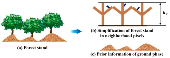
Figure 1.
Simplification of a forest stand in the neighborhood pixels.
We summarize the above description with the following assumptions:
(1) The forest height remains unchanged within neighboring pixels; (2) the residual ground height can be considered consistent within neighboring pixels; (3) the coefficients of the FL polynomials remain unchanged within neighboring pixels, except for the last polynomial coefficient; and (4) the vertical profile of the forest volume is different with different polarizations.
The polarimetric complex interferometric coherence can be related to the FL polynomials of Equation (3) in the framework of single-baseline full polarization. Here, we take the third-order FL polynomials as an example:
where w = 1, 2, ..., m; hg represents the ground height; p is the p-th row in the neighboring pixels, where p = 1, 2, ..., P; and q is the q-th column in the neighboring pixels, where q = 1, 2, ..., Q. In this case, the number of unknowns is 2 + m(n − 1) + PQm.
Determining the order of the FL polynomials is an important step for forest height estimation. The order of the FL polynomials determines the ability to describe the resolution of the vertical profile of the forest volume. In this study, we estimated the forest height by the use of the neighboring pixels and multi-polarizations under the framework of single-baseline PolInSAR data. Thus, the order of the FL polynomials can be calculated by (4) the following:
where m represents the number of polarizations.
According to Equation (11), the number of polarizations in forest height estimation is also worth investigating. The polarization selection has been described in [20], but we still suggest the use of phase diversity (PD)-optimized polarizations for the forest height estimation. By maximizing the phase difference between polarizations, PDHigh represents the volume-dominated scattering polarization, and PDLow represents the ground-dominated scattering polarization.
At the same time, with the increase in the pixel number, the order of the FL polynomials can also increase. That is to say, there can be a very high resolution for the vertical profile function of the forest volume. For instance, we can obtain ninth-order FL polynomials at most with m = 2 and PQ = 9, which is far beyond the third-order FL polynomials required for forest biomass estimation [14,19]. Nevertheless, with the increasing pixel numbers, the ability for the reconstruction of the forest volume vertical structural details is improved, while we lose the spatial resolution. How to balance the resolution of the forest volume reconstruction and the spatial resolution of the interferogram is a problem that is worthy of investigation. However, in this article, we do not pay too much attention to this contradiction, and the forest height is estimated with the 3 × 3 neighboring pixels.
Finally, the unknown parameters can be calculated by a non-linear least-squares optimization algorithm, and the corresponding objective function is
In order to obtain satisfactory forest height estimation results by the non-linear least-squares optimization algorithm, we need to provide reliable initial values and reasonable upper and lower bounds. In this study, the initial values were calculated as follows:
- (1)
- Forest height: The forest height of every pixel can be obtained by the three-stage inversion algorithm under the framework of the RVoG model [34]. The mean forest height is then calculated as the approximate values of the forest height within p × q pixels.
- (2)
- Ground height: According to Section 2.3, we set the initial value of the ground height to 0.
- (3)
- Coefficients of the FL polynomials: The coefficients of the FL polynomials can be obtained by the method proposed in [9,20].
- (4)
- Upper and lower bounds of the forest height: The bounds of the forest height are set to 0.5h0 ≤ hv ≤ 1.5h0, where h0 represents the approximate value of the forest height [17,20,30].
4. Results
In order to validate the performance of the proposed forest canopy height inversion model, we selected the Mabounie region of Gabon in Africa as the first study area. The area is about 180 km away from the airport of Libreville, the capital city of Gabon, and the main vegetation types in the Mabounie experimental area are mature primary tropical forests and some degraded tropical rainforests, of which the mature forests mainly have tree heights of 40–60 m, and the degraded forests mainly have tree heights of 20 m. The Mabounie experimental area is an important experimental site for tropical rainforest research, and the ground survey data and LiDAR data are complete, which can provide sufficient data guarantee for the experimental validation of the algorithm proposed in this paper. We selected two airborne P-band multi-polarization SAR images obtained in the AfriSAR campaign in 2016 to verify the accuracy of the proposed method. The main details of the interferometric pair are listed in Table 1. Moreover, in this study area, LiDAR data have also been collected by the National Aeronautics and Space Administration Land, Vegetation, and Ice Sensor (LVIS), and were used to validate the forest height estimation results [35].

Table 1.
The main details of the Mabounie interferometric pair.
Polarimetric SAR images 1 and 2 formed an interferometric pair. For the interferometric pair, a series of PolInSAR preprocessing steps were executed, including image co-registration, flat-earth removal, and multi-look processing [9]. We then used the PD optimization method to estimate the polarimetric coherences. The scale of the multi-look processing was set to 4 × 2 (azimuth/range), and the window size for the coherence estimation was set to 11 × 11. Finally, we obtained the PDHigh polarimetric coherences and PDLow polarimetric coherences.
In this study, we estimated the forest height by the FL model within the 3 × 3 neighboring pixels, and the number of complex observations was 18. Meanwhile, the number of unknown parameters was 24. Concretely, the unknown parameters were the forest height hv, the ground height hg, and the coefficients of the FL polynomials: a10(PDHigh), a20(PDHigh), , a10(PDLow), a20(PDLow), and .
Figure 2a shows the forest height estimated from the RVoG model, Figure 2b shows the forest height estimated by the third-order FL model with neighboring pixels, and Figure 2c shows the LiDAR forest height product. It can be seen that the forest height estimated by the third-order FL model is closer to the LiDAR product. The results also show a left-to-right trend. The main reason for this trend is the variation of kz along the range direction since the incidence angle increases along the range direction for an airborne system [36].
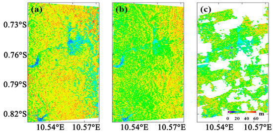
Figure 2.
(a) RVoG model forest height estimation results in the the Mabounie region. (b) The forest height results estimated by the third-order FL model with 3 × 3 neighboring pixels in the the Mabounie region. (c) The LiDAR forest height product in the the Mabounie region.
The root-mean-square error (RMSE) is widely used for accuracy assessment in tasks such as forest canopy height inversion [31]. In order to further analyze the performance of the different models, the root-mean-square error (RMSE) was calculated with respect to the LiDAR forest height product. A total of 1170 forest stands were uniformly selected, where the size of each stand was 51 × 51 pixels [20,30,31]. The RMSE of the RVoG model is 5.28 m, and the RMSE of the third-order FL model with 3 × 3 neighboring pixels is 4.32 m, which are shown in Figure 3. The accuracy of the forest height estimation by the third-order FL model is improved by 18% when compared with the RVoG model. According to the RMSE, it can be stated that the third-order FL model is superior to the RVoG model in forest height estimation. The tree species in the Mabounie area are mainly tropical species, and the vertical distribution of the canopy scatterers can be complicated. Meanwhile, in the field of low-frequency radar, the forest scatterers are branches with anisotropy. In this configuration, the hypothesis of a uniform canopy, as required by the RVoG model, may no longer be appropriate. In contrast, the forest vertical profile described by the third-order FL polynomials is more consistent with the forest at Mabounie.
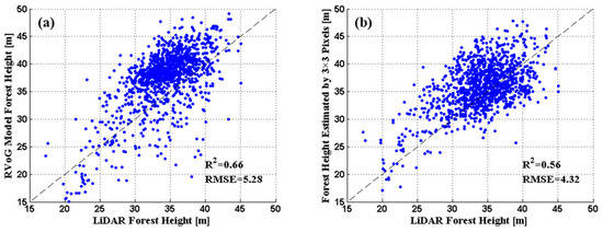
Figure 3.
(a) Mabounie area RVoG model forest height estimation results cross-validated with the LiDAR product. (b) Cross-validation plot of the forest height estimation results of the third-order FL model with the LiDAR product for the Mabounie area.
5. Discussion
In this section, we describe the experiments conducted to evaluate the generalizability of the proposed forest canopy height inversion model in different types of forest canopy height inversion tasks. The second point of discussion is constructed based on the FL polynomial forest height estimation algorithm based on a single-baseline configuration, as described in Section 4 and is used to discuss the effect of different orders of FL polynomials on forest canopy height inversion. Finally, in Section 5.3, we describe the limitations of the model proposed in this study and potential future research.
5.1. Inversion of Forest Canopy Height in a Boreal Forest Area by the Model Proposed in This Article
As was demonstrated in Section 3, the proposed FL polynomial forest height estimation algorithm based on a single-baseline configuration can obtain more accurate inversion results in the forest canopy height inversion task than the RVoG model. It is worth noting that the first study area was a tropical rainforest region, where the vertical structure of the forest is easier to characterize, the forest area is more homogeneous, and because of the flat understory topography of the area, there are fewer surface phases remaining after removing the surface phases, which makes the inversion of the forest canopy height easy. In order to study the performance of the model in forest canopy height inversion in different types of forest areas, the model proposed in this article was used as a model for forest canopy height inversion in a different forested area. We chose the Krycklan region of Sweden, located at a high latitude in the Northern Hemisphere, as a study area (64°14′N, 19°46′E). The predominant forest type in this area is boreal forest. The average forest height in this area is about 18 m. Two P-band polarization SAR images acquired during the BioSAR 2008 campaign were used to verify the effectiveness of the proposed algorithm. The main forest types in the study area are mixed coniferous and broadleaf forests, with Scots pine and Norway spruce as the main species of coniferous forests and a few birches as the main species of broadleaf forests and the highest forest height of about 35 m. The Krycklan River basin belongs to the mountainous-hilly region, with a moderately varying topographic gradient and a ground level that ranges from 150 m to 380 m above sea level. The main details of the Interferometric pair are listed in Table 2. The LiDAR forest height product for this area was used to analyze the performance of the algorithm proposed in this article.
Table 2.
The main details of the Krycklan interferometric pair.
For the interferometric pair, the preprocessing steps were the same as for the Mabounie SAR data, except that the scale of the multi-look processing was set to 2 × 1.
Figure 4a shows the RVoG model forest height estimation results, Figure 4b shows the results of the third-order FL model with 3 × 3 neighboring pixels, and Figure 4c shows the LiDAR forest height product, which was used for the accuracy verification. According to Figure 4, it is apparent that the RVoG model and third-order FL model show the same trend of forest height estimation results, but the third-order FL model is closer to the LiDAR forest height product.
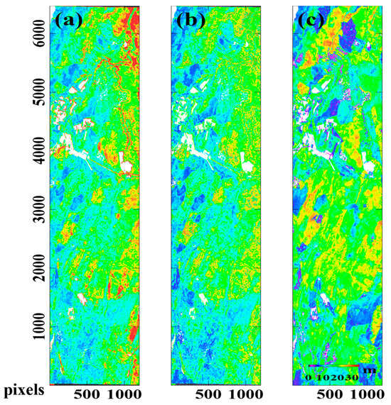
Figure 4.
(a) RVoG model forest height estimation in the the Krycklan region. (b) The forest height results estimated by the third-order FL model with 3 × 3 neighboring pixels in the the Krycklan region. (c) The LiDAR forest height product in the the Krycklan region.
Moreover, the RMSE was calculated with respect to the LiDAR forest height product, for which we selected 1318 forest stands in this area [20,30,31]. Firstly, we note that the RMSE of the RVoG model is 4.67 m, and the RMSE of the third-order FL model is 3.88 m. The results of the cross-validation show that the performance of the single-baseline algorithm proposed in this article is improved by 16.7% when compared to the RVoG model. However, it can be seen from Figure 4 and Figure 5 that the algorithm proposed in this article shows overestimation in the low forest areas and underestimation in the high forest areas.
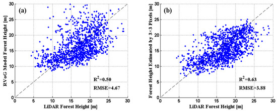
Figure 5.
(a) Cross-validation plot of the RVoG model forest height estimation results with the LiDAR product. (b) Cross-validation plot of the third-order FL model forest height estimation results with the LiDAR product.
5.2. Effects of Fourier–Legendre Polynomials of Different Orders on Forest Canopy Height Inversion
Although the previous experiments proved that the use of third-order FL polynomials can satisfy the vertical distribution of forest scatterers, which in turn meets the needs of forest biomass estimation, theoretically, when the FL polynomials are used to describe the vertical distribution of forest canopy scatterers, the polynomials should be set to a high order as much as possible. This is because the higher-order FL polynomial functions are more complex and can more accurately describe the details of the forest vertical structure while accurately describing the main body of the forest vertical structure. This detailed information on the vertical structure of forests, including trunks, branches, etc., is positively useful for obtaining information on the vertical structure and biomass of forests on a large scale. Therefore, in this section, in order to investigate the effect of different orders of FL polynomials in forest canopy height inversion, we describe the forest canopy height inversion experiments conducted for the Mabounie rainforest experimental area and the Krycklan boreal forest experimental area by using FL polynomials of the third order, the fourth order, and the fifth order. In this article, based on a spatial domain of 9 pixels (3 × 3 pixels, with a spatial resolution of about 4.5 m in Mabounie and 11.0 m in Krycklan), we briefly attempt to describe the vertical distribution of the forest canopy scatterers using fourth-order FL polynomials and fifth-order FL polynomials. Based on this, PolInSAR height inversion was conducted, taking into account the non-uniform distribution of branches in the forest canopy, as shown in Figure 6 and Figure 7.
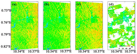
Figure 6.
PolInSAR forest height inversion results based on third-, fourth-, and fifth-order Fourier–Legendre (FL) polynomials describing the vertical distribution of the forest canopy scatterers and the LiDAR forest height product covering part of the Mabounie area. (a) The forest height inversion results based on third-order FL polynomials describing the vertical distribution of the forest canopy scatterers. (b) The forest height inversion results describing the vertical distribution of the forest canopy scatterers based on fourth-order FL polynomials. (c) The forest height inversion results describing the vertical distribution of the forest canopy scatterers based on fifth-order FL polynomials. (d) The LiDAR forest height product covering a part of the experimental area.
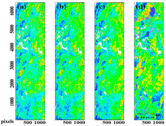
Figure 7.
PolInSAR forest height inversion results based on third-, fourth-, and fifth-order FL polynomials describing the vertical distribution of the forest canopy scatterers, as well as the LiDAR forest height product covering a portion of the Krycklan region. (a) The forest height inversion results based on third-order FL polynomials describing the vertical distribution of the forest canopy scatterers. (b) The forest height inversion results describing the vertical distribution of the forest canopy scatterers based on fourth-order FL polynomials. (c) The forest height inversion results describing the vertical distribution of the forest canopy scatterers based on fifth-order FL polynomials. (d) The LiDAR forest height product covering part of the experimental area.
On the whole, based on the region of 9 pixels, the trend of the PolInSAR forest height inversion results are basically the same when FL polynomials of different orders are used to describe the vertical structure of the scatterers in the forest canopy. The main reason for this phenomenon is that the FL polynomials are orthogonal, and the addition and deletion of one term have no effect on the other terms, i.e., when the coefficients of the higher-order FL polynomials are zero or tend to zero, the higher-order polynomials can degenerate into lower-order FL polynomials.
In order to quantitatively characterize the accuracy of the forest height inversion, based on the 1170 forest stands selected as described in Section 4 and 1318 forest stands selected as described in Section 5.1, the RMSE and correlation coefficient (R2) were used as the measures of accuracy for the forest height inversion results, as shown in Figure 8 and Figure 9.
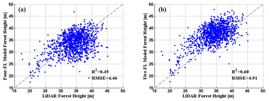
Figure 8.
Cross-validation plots of the cross-validation results of the PolInSAR forest height inversion results with the sample plots of the LiDAR forest height product covering part of the Mabounie area. (a) Cross-validation plot of the forest height inversion results based on fourth-order FL polynomials describing the vertical distribution of the forest canopy scatterers with sample plots of the LiDAR forest height product. (b) Cross-validation plot of the forest height inversion results based on fifth-order FL polynomials describing the vertical distribution of the forest canopy scatterers with sample plots of the LiDAR forest height product.
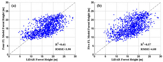
Figure 9.
Cross-validation plots of the cross-validation results of the PolInSAR forest height inversion results with sample plots of the LiDAR forest height product covering part of the Krycklan area. (a) Cross-validation plot of the forest height inversion results based on fourth-order FL polynomials describing the vertical distribution of the forest canopy scatterers with sample plots of the LiDAR forest height product. (b) Cross-validation plot of the forest height inversion results based on fifth-order FL polynomials describing the vertical distribution of the forest canopy scatterers with sample plots of the LiDAR forest height product.
From the results, it can be seen that the RMSEs corresponding to the forest height inversion results of single-baseline PolInSAR are 4.46 m and 4.91 m in the Mabounie region and 3.90 m and 4.08 m in the Krycklan region, respectively. Although the RMSEs are at the same level of accuracy, the accuracy of the forest height inversion decreases as the order of the FL polynomial increases. The main reason for this phenomenon is that, when the higher-order FL polynomials are used, although the vertical structure of the forest vegetation can be described more accurately, the value of the higher-order expansion term fi tends to be close to 0, and the number of observation matrix conditions associated with the higher-order expansion term fi is larger. This makes the parameter inversion process more sensitive to observation errors (e.g., temporal decoherence, spatial decoherence, etc.), which ultimately leads to a decrease in the accuracy of the forest height inversion.
5.3. Limitations and Future Research
In this article, we have proposed the use of FL polynomials to model the expression for the distribution of forest canopy scatterers in the vertical direction. We conducted experiments based on different forest types and obtained more accurate inversion results for forest canopy height. However, the proposed method still has some limitations. Firstly, the most suitable Fourier polynomials cannot be determined at present. Although we obtained third-, fourth-, and fifth-order FL polynomial inversion results according to the different forest types in the study areas, the errors of these results were convergent due to the fact that the propagation process of electromagnetic waves inside the forest canopy is complex. Furthermore, at the same time, the vertical structure of the forest canopy is lacking in a priori information. Therefore, it is not possible to determine the optimal FL polynomial order. Secondly, choosing the optimal number of neighborhood pixels is also very difficult. As the number of neighborhood pixels increases, the ability to reconstruct the details of the vertical structure of the forest volume improves. For example, when the neighborhood region consists of 3 × 3 pixels, the highest order can be extended to the ninth order, even if only two polarization methods are applied for the forest height inversion. However, the spatial resolution will be lost. At the same time, the ninth-order FL coefficient is not necessarily optimal. In future studies, we will use LiDAR to analyze and test data from different types of forest areas, and use the results as a priori information to determine the optimal Fourier polynomial order and the most appropriate number of neighborhood pixels. Thirdly, there may be differences in the vertical structure of different tree species, and the types of trees within the coverage of neighboring pixels may be different, which was not taken into account in this study. In addition, when constructing the single-baseline Fourier polynomial forest canopy height inversion model, we will use principal component analysis (PCA) to consider the information of the dominant species in the neighboring pixels and divide the neighboring pixel areas according to the different species for forest height inversion.
6. Conclusions
In this article, we have proposed an FL polynomial forest height estimation algorithm based on a single-baseline configuration. The main idea is that it is possible to estimate the forest height without losing the spatial resolution. This is based on the assumption that the forest height, the ground height, and the vertical profile of the forest volume remain unchanged within the neighboring pixels. The P-band experimental results showed that the method proposed in this article is feasible and effective.
A square area is typically used to carry out sub-area experiments. However, the ground height and the vertical profile of the forest volume may be different in this sub-area. Therefore, which shapes are appropriate to distinguish the sub-area needs to be investigated in the future. Meanwhile, the temporal decorrelation cannot be ignored in the repeat-pass configuration, so how to compensate for the influence of the temporal effect also needs to be investigated.
Author Contributions
Conceptualization, B.Z. and H.Z.; methodology, B.Z.; software, X.C. and W.X.; validation, W.S., J.Z. and B.Z.; formal analysis, B.Z.; investigation, B.Z.; writing—original draft preparation, B.Z.; writing—review and editing, H.Z.; visualization, J.Z.; supervision, S.X.; project administration, B.Z.; funding acquisition, B.Z. All authors have read and agreed to the published version of the manuscript.
Funding
This work was supported in part by the National Natural Science Foundation of China under Grant 42204031 and a project funded by the China Postdoctoral Science Foundation (2022MD723791).
Data Availability Statement
The data presented in this study are available on request from the corresponding author.
Acknowledgments
We are very grateful to all the reviewers, institutions, and researchers for their help and advice on our work.
Conflicts of Interest
The authors declare no conflict of interest.
References
- Pan, Y.; Birdsey, R.A.; Fang, J.; Houghton, R.; Kauppi, P.E.; Kurz, W.A.; Phillips, O.L.; Shvidenko, A.; Lewis, S.L.; Canadell, J.G.; et al. A large and persistent carbon sink in the world’s forests. Science 2011, 333, 988–993. [Google Scholar] [CrossRef] [PubMed]
- Houghton, R.A.; Hall, F.; Goetz, S.J. Importance of biomass in the global carbon cycle. J. Geophys. Res. Biogeosci. 2015, 114, G00E03. [Google Scholar] [CrossRef]
- Solberg, S.; Astrup, R.; Gobakken, T.; Næsset, E.; Weydahl, D.J. Estimating spruce and pine biomass with interferometric X-band SAR. Remote Sens. Environ. 2010, 114, 2353–2360. [Google Scholar] [CrossRef]
- Fu, H.; Zhu, J.; Wang, C.; Li, Z. Underlying topography extraction over forest areas from multi-baseline PolInSAR data. J. Geod. 2018, 92, 727–741. [Google Scholar] [CrossRef]
- Huang, H.; Liu, C.; Wang, X.; Biging, G.S.; Chen, Y.; Yang, J.; Gong, P. Mapping vegetation heights in China using slope correction ICESat data, SRTM, MODIS-derived and climate data. ISPRS J. Photogramm. Remote Sens. 2017, 129, 189–199. [Google Scholar] [CrossRef]
- Liao, Z.; He, B.; Shi, Y. Improved forest biomass estimation based on P-band repeat-pass PolInSAR data across different forest sites. Int. J. Appl. Earth Obs. Geoinf. 2022, 115, 103088. [Google Scholar] [CrossRef]
- Schlund, M.; Baron, D.; Magdon, P.; Erasmi, S. Canopy penetration depth estimation with TanDEM-X and its compensation in temperate forests. ISPRS J. Photogramm. Remote Sens. 2019, 147, 232–241. [Google Scholar] [CrossRef]
- Zhang, Q.; Ge, L.; Hensley, S.; Metternicht, G.I.; Liu, C.; Zhang, R. PolGAN: A deep-learning-based unsupervised forest height estimation based on the synergy of PolInSAR and LiDAR data. ISPRS J. Photogramm. Remote Sens. 2022, 186, 123–139. [Google Scholar] [CrossRef]
- Treuhaft, R.N.; Madsen, S.N.; Moghaddam, M.; van Zyl, J.J. Vegetation characteristics and underlying topography from interferometric radar. Radio Sci. 1996, 31, 1449–1485. [Google Scholar] [CrossRef]
- Freeman, A.; Durden, S.L. A three-component scattering model for polarimetric SAR data. IEEE Trans. Geosci. Remote Sens. 1998, 36, 963–973. [Google Scholar] [CrossRef]
- Cloude, S.R. Polarisation Applications in Remote Sensing; Oxford University Press: New York, NY, USA, 2009. [Google Scholar]
- Cloude, S.R.; Papathanassiou, K.P. Polarimetric SAR interferometry. IEEE Trans. Geosci. Remote Sens. 1998, 36, 1551–1565. [Google Scholar] [CrossRef]
- Papathanassiou, K.P.; Cloude, S.R. Single-baseline polarimetric SAR interferometry. IEEE Trans. Geosci. Remote Sens. 2001, 39, 2352–2363. [Google Scholar] [CrossRef]
- Freeman, A. Fitting a two-component scattering model to polarimetric SAR data from forests. IEEE Trans. Geosci. Remote Sens. 2007, 45, 2583–2592. [Google Scholar] [CrossRef]
- Kugler, F.; Lee, S.-K.; Papathanassiou, K.P. Estimation of forest vertical structure parameter by means of multi-baseline Pol-InSAR. In Proceedings of the IEEE International Geoscience and Remote Sensing Symposium, Cape Town, South Africa, 12–17 July 2009; pp. 721–724. [Google Scholar]
- Garestier, F.; Le Toan, T. Forest modeling for height inversion using single-baseline InSAR/Pol-InSAR data. IEEE Trans. Geosci. Remote Sens. 2010, 48 Pt 2, 1528–1539. [Google Scholar] [CrossRef]
- Fu, H.; Wang, C.; Zhu, J.; Xie, Q.; Zhang, B. Estimation of Pine Forest Height and Underlying DEM Using Multi-Baseline P-Band PolInSAR Data. Remote Sens. 2016, 8, 820. [Google Scholar] [CrossRef]
- Garestier, F.; Le Toan, T. Estimation of the Backscatter Vertical Profile of a Pine Forest Using Single Baseline P-Band (Pol-)InSAR Data. IEEE Trans. Geosci. Remote Sens. 2010, 48, 3340–3348. [Google Scholar] [CrossRef]
- Fu, W.; Guo, H.; Song, P.; Tian, B.; Li, X.; Sun, Z. Combination of PolInSAR and LiDAR techniques for forest height estimation. IEEE Geosci. Remote Sens. Lett. 2017, 14, 1218–1222. [Google Scholar] [CrossRef]
- Zhang, B.; Fu, H.; Zhu, J.; Peng, X.; Xie, Q.; Lin, D.; Liu, Z. A Multibaseline PolInSAR Forest Height Inversion Model Based on Fourier-Legendre Polynomials. IEEE Geosci. Remote Sens. Lett. 2021, 18, 687–691. [Google Scholar] [CrossRef]
- Tebaldini, S.; Rocca, F. Multibaseline Polarimetric SAR Tomography of a Boreal Forest at P- and L-Bands. IEEE Trans. Geosci. Remote Sens. 2012, 50, 232–246. [Google Scholar] [CrossRef]
- Peng, X.; Li, X.; Du, Y. Forest Height Estimation from a Robust TomoSAR Method in the Case of Small Tomographic Aperture with Airborne Dataset at L-Band. Remote Sens. 2021, 13, 2147. [Google Scholar] [CrossRef]
- Peng, X.; Wang, Y.; Long, S.; Pan, X.; Zhu, J.; Li, X. Underlying Topography Inversion Using TomoSAR Based on Non-Local Means for an L-Band Airborne Dataset. Remote Sens. 2021, 13, 2926. [Google Scholar] [CrossRef]
- Wang, Y.; Xie, Q.; Li, X.; Luo, X.; Du, Y.; Zhang, B. Underlying topography and forest height estimation from SAR tomography based on a nonparametric spectrum estimation method with low sidelobes. Int. J. Digit. Earth 2022, 15, 2184–2201. [Google Scholar] [CrossRef]
- Cloude, S.R. Dual-Baseline Coherence Tomography. IEEE Geosci. Remote Sens. Lett. 2007, 4, 127–131. [Google Scholar] [CrossRef]
- Cloude, S.R. Polarization coherence tomography. Radio Sci. 2016, 41, 1–27. [Google Scholar] [CrossRef]
- Ghasemi, N.; Tolpekin, V.; Stein, A. A modified model for estimating tree height from PolInSAR with compensation for temporal decorrelation. Int. J. Appl. Earth Obs. Geoinf. 2018, 73, 313–322. [Google Scholar] [CrossRef]
- Ghasemi, N.; Tolpekin, V.A.; Stein, A. Estimating Tree Heights Using Multibaseline PolInSAR Data with Compensation for Temporal Decorrelation, Case Study: AfriSAR Campaign Data. IEEE J. Sel. Top. Appl. Earth Obs. Remote Sens. 2018, 11, 3464–3477. [Google Scholar] [CrossRef]
- Caicoya, A.T.; Kugler, F.; Papathanassiou, K.; Biber, P.; Pretzsch, H. Biomass estimation as a function of vertical forest structure and forest height. Potential and limitations for Radar Remote Sensing. In Proceedings of the 8th European Conference on Synthetic Aperture Radar (EUSAR 2010), Aachen, Germany, 7–10 June 2010; pp. 901–904. [Google Scholar]
- Zhang, B.; Fu, H.; Zhu, J.; Peng, X.; Lin, D.; Xie, Q.; Hu, J. Forest Height Estimation Using Multi-Baseline Low-Frequency PolInSAR Data Affected by Temporal Decorrelation. IEEE Geosci. Remote Sens. Lett. 2021, 19, 99. [Google Scholar] [CrossRef]
- Xie, Q.; Zhu, J.; Wang, C.; Fu, H.; Lopez-Sanchez, J.M.; Ballester-Berman, J.D. A modified dual-baseline PolInSAR method for forest height estimation. Remote Sens. 2017, 9, 819. [Google Scholar] [CrossRef]
- Tobler, W.R. A Computer Movie Simulating Urban Growth in the Detroit Region. Econ. Geogr. 1970, 46, 234–240. [Google Scholar] [CrossRef]
- Avitabile, V.; Camia, A. An assessment of forest biomass maps in Europe using harmonized national statistics and inventory plots. For. Ecol. Manag. 2018, 409, 489–498. [Google Scholar] [CrossRef]
- Cloude, S.R.; Papathanassiou, K.P. Three-stage inversion process for polarimetric SAR interferometry. IEEE Proc.-Radar Sonar Navig. 2003, 150, 125–134. [Google Scholar] [CrossRef]
- Disclaim Fatoyinbo, T.; Armston, J.; Simard, M.; Saatchi, S.; Denbina, M.; Lavalle, M.; Hofton, H.; Tang, H.; Marselis, S.; Pinto, N.; et al. The NASA AfriSAR campaign: Airborne SAR and LiDAR measurements of tropical forest structure and biomass in support of current and future space missions. Remote Sens. Environ. 2021, 264, 112533. [Google Scholar] [CrossRef]
- Kugler, F.; Lee, S.K.; Hajnsek, I.; Papathanassiou, K.P. Forest Height Estimation by Means of Pol-InSAR Data Inversion: The Role of the Vertical Wavenumber. IEEE Trans. Geosci. Remote Sens. 2015, 53, 5294–5311. [Google Scholar] [CrossRef]
Disclaimer/Publisher’s Note: The statements, opinions and data contained in all publications are solely those of the individual author(s) and contributor(s) and not of MDPI and/or the editor(s). MDPI and/or the editor(s) disclaim responsibility for any injury to people or property resulting from any ideas, methods, instructions or products referred to in the content. |
© 2023 by the authors. Licensee MDPI, Basel, Switzerland. This article is an open access article distributed under the terms and conditions of the Creative Commons Attribution (CC BY) license (https://creativecommons.org/licenses/by/4.0/).