Forest Carbon Density Estimation Using Tree Species Diversity and Stand Spatial Structure Indices

Abstract

The forest spatial structure and diversity of tree species, as the important evaluation indicators of forest quality, are key factors affecting forest carbon storage. To analyze the impacts of biodiversity indices and stand spatial structure on forest carbon density, five tree diversity indices were calculated from three aspects of richness, diversity and evenness, and three indices (Reineke’s stand density index, Hegyi’s competition index and Simple mingling degree) were calculated from stand spatial structure. The relationships between these eight indices and forest carbon density were explored using the Structural Equation Model (SEM). Then, these eight indices were used as characteristic variables to predict the aboveground carbon density of trees (abbreviated as forest carbon density) in the sample plots of the National Forest Resources Continuous Inventory (NFCI) in Shaoguan City in 2017. Multiple Linear Regression (MLR) and four typical machine learning models of Random Forest (RF), Tree-based Piecewise Linear Model (M5P), Artificial Neural Network (ANN) and Support Vector Regression (SVR) were used to predict the forest carbon density. The results show that: (1) Based on the analysis results of the structural equation model (SED), the species diversity and forest stand spatial structure have greater impacts on carbon density. (2) The R² of all the five prediction models is greater than 0.6, among which the random forest model is the highest. (3) Based on the calculation results of optimal model of RF, the mean forest carbon density of Shaoguan city in 2017 was 43.176 tC/ha. The forest carbon density can be accurately estimated based on the species diversity index and stand spatial structure with machine learning algorithms. Therefore, a new method for the prediction of forest carbon density and carbon storage using species diversity indices and stand spatial structure can be explored. By analyzing the impacts of different biodiversity indices and stand spatial structure on forest carbon density, a scientific reference for the making of management measures for increasing forest carbon sinks and reducing emissions can be provided.

1. Introduction

With the intensification of human activities’ impacts on the environment, greenhouse gas concentrations are increasing, the ozone layer is being damaged, global warming is occurring, and extreme weather events are occurring frequently. To address the issue of global climate change, the United Nations formulated the United Nations Framework Convention on Climate Change in 1992 to comprehensively control CO₂ emissions [1]. The Intergovernmental Panel on Climate Change’s sixth assessment report further confirms the impact of human activities on the atmosphere, oceans and land, which is contributing to climate change [2]. With ongoing global warming, climate change is expected to intensify further. Global carbon cycles have become one of the core issues of global climate change research [3]. The primary component of terrestrial ecosystems is forest ecosystems [4,5] which fix around two-thirds of the terrestrial ecosystems’ carbon every year, making them the largest carbon pool on land. Since the carbon sequestration capacity of forests is essential for reducing atmospheric CO₂ concentrations and mitigating global warming, forest ecosystems play an important role in the global carbon cycle [6,7].

As a crucial component of forest ecosystems, species diversity is the material basis for maintaining the function and stability of forest ecosystems and providing ecological services [8]. Since trees are the main component of the forest ecosystem, tree species diversity largely represents the level of forest biological diversity at the stand scale. Tree species diversity is a key factor affecting stability, productivity and carbon storage [9]. Yin et al. [10] studied the driving factors of subtropical forest carbon storage, and the results showed that biodiversity was one of the influencing factors. Huang et al. [11] conducted experiments in subtropical forest area and found that tree species diversity could influence forest productivity and carbon storage. Con et al. [12] investigated the relationship between aboveground biomass and the multiple indices of biodiversity in tropical forests of Vietnam and found that aboveground biomass was positively correlated with species richness, Shannon diversity index, and evenness. Vance et al.’s [13] research determined aboveground biomass was positively correlated with measures of species diversity (i.e., species richness, Shannon diversity index and Simpson diversity index) in subtropical forests of Puerto Rico. Shahid et al.’s [14] research showed that species richness and the Shannon–Weiner index were correlated with carbon stocks. Kumar et al. [15] analyzed the relationship between species richness and aboveground carbon stocks and concluded that preserving species richness was crucial for maintaining aboveground carbon stocks in forest ecosystems.

In addition, in forests with high tree species richness, the growth competition among tree species is more intense, leading to more active absorption and fixation of CO₂ by trees. The species diversity can also improve the fertility and water conservation capacity of forest soil, promoting plant growth and carbon sequestration further. Compared with forest ecosystems with relatively low species diversity, those with high species diversity not only have a faster carbon cycle rate, but also can store more carbon in both the aboveground and underground [16]. Canopy density and species diversity show a significant positive correlation, and tree height and diameter at breast height (DBH) show a significant correlation with species diversity of the tree [17]. The height and DBH of the tree directly determine the aboveground biomass of the forest and further determine the aboveground carbon density of the forest. Because species diversity affects tree photosynthesis, reflects soil fertility and water status, and is significantly related to the DBH and height of trees, it may be feasible to estimate forest carbon density based on species diversity, but there are still gaps in current research on the prediction of carbon density using species diversity indices.

The forest carbon density is a comprehensive reflection of forest structure, which determines the competitive potential and spatial ecological niche of trees. To a large extent, forest structure determines the stability, succession direction and management space of the forest stand. Forest structure and inherent patterns influence and constrain the carbon sequestration function of the forest. Forest structure consists of spatial and non-spatial structures, in which forest spatial structure mainly refers to the degree of distribution, intermixing, and competition of trees within a forest ecosystem. Hall et al. [18] incorporated forest structure into a forest aboveground biomass model and found that this model was more accurate than models based solely on empirical data. Zheng et al. [19] developed a polynomial model that combined spectral variables from land satellite imagery with forest age, which improved the prediction accuracy of forest aboveground biomass. Ou et al. [20] improved the accuracy of forest aboveground biomass estimation in high-mountain pine forests by including dummy variables of age classes in their model. Subtropical forests, due to their favorable hydrothermal conditions, diverse tree species, and complex forest spatial structure, are a major source of errors and uncertainties in estimating forest carbon density. Therefore, incorporating forest spatial structure into estimation models can improve the estimation accuracy of forest carbon density to some extent.

The subtropical forest has a special status in the global ecological environment and plays an important role in the carbon cycle of the global terrestrial ecosystem. China’s subtropical forest is a unique global forest ecosystem at the same latitude, with multiple forest types, various species and high forest productivity [21]. As an important component of the collective-owned forest region in Southern China, the forest in Shaoguan has the characteristics of high forest coverage and rich biodiversity. Although the forest resources in Shaoguan have been in a steady state of growth, due to frequent human activities, the accelerating process of urbanization and industrialization and related forestry policies, there are still some problems existing in regional forests, such as uneven spatial distribution of forest, low unit stock volume, unreasonable forest types and age class structure. The study of forest carbon density predication and its influencing factors has important practical significance to the making of regional management measures for increasing forest sinks and reducing emissions.

Although there are many factors included in the NFCI sample investigation, many of which are closely related to biodiversity and forest structure, the investigation does not include biomass or carbon density. Currently, most research on the prediction of forest carbon density at or above the county level is based on remote sensing images, with few studies on the relationship between species diversity, stand spatial structure and forest carbon density, not to mention carbon density predictions based on diversity indices or stand spatial structure indices. This paper calculates five tree species diversity indices which include the Patrick index (S), Shannon index (H), Simpson index (D), Inverse Simpson index (D₀), Pielou’s Evenness index (J) and three stand spatial structure factors including Reineke’s stand density index (SDI), Hegyi’s competition index (CI) and Simple mingling degree (M) from NFCI data in Shaoguan in 2017, and builds MRL and four typical machine learning models, RF, M5P, ANN and SVR models, so as to predict forest carbon density with eight indies as the independent variable. The primary objectives of this paper are: (1) to analyze the impacts of biodiversity indices and stand spatial structure factors on forest carbon density; (2) to explore and propose a method for predicting forest carbon density based on forest tree species diversity indices and stand spatial structure factors; and (3) to put forward several suggestions on forest management for increasing carbon sequestration and reducing emission.

2. Materials and Methods

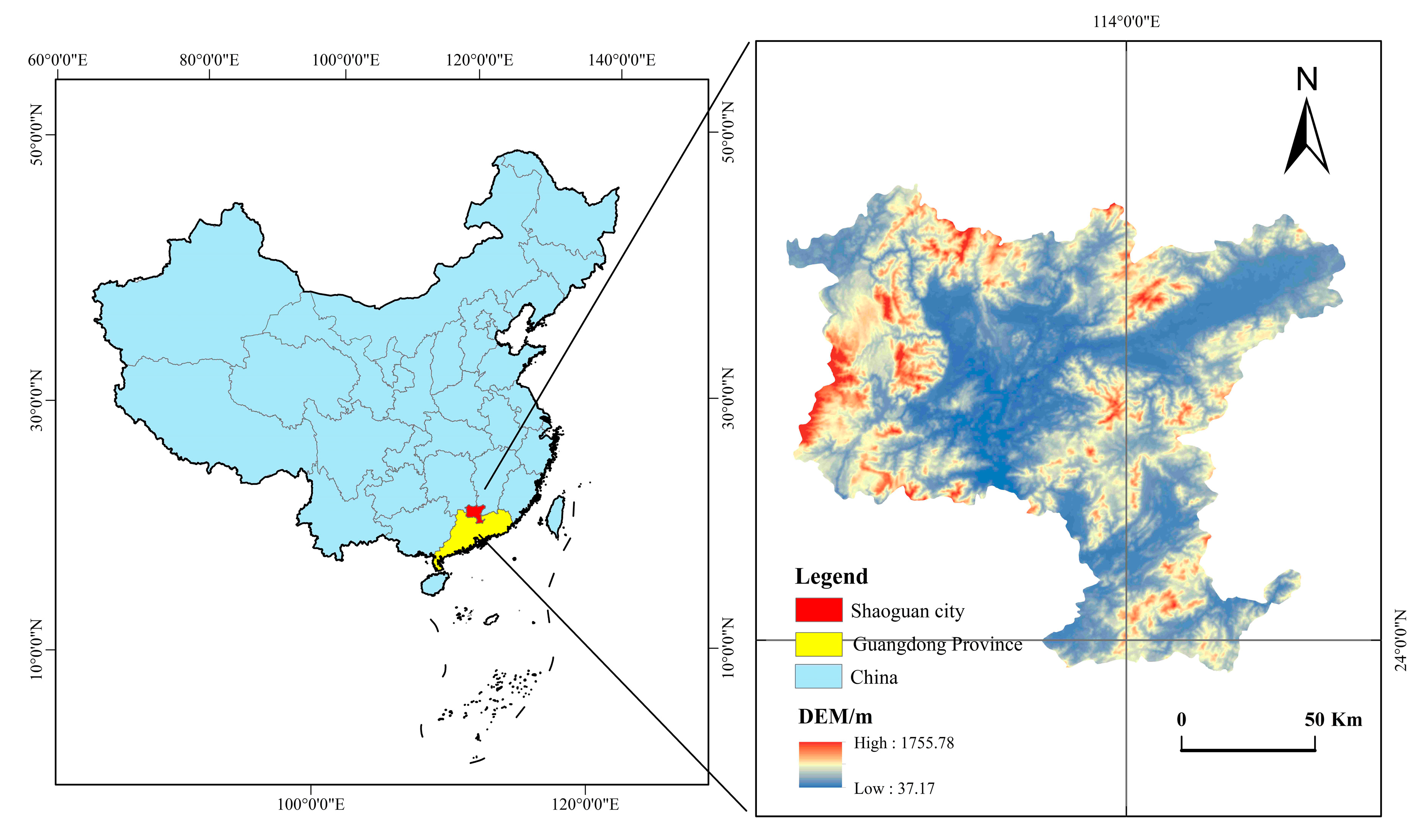
2.1. Study Area

Shaoguan city is located in the northeast part of Guangdong Province, China. The whole territory is located between 23°53′–25°31′ N and 112°53′–114°45′ E (Figure 1). The types of landform in Shaoguan are complex and diverse, including mountains, hills, tablelands and plains. The terrain is generally high in the north and low in the south, with many mountains and high hills in the north. The spatial and temporal distribution of water resources in Shaoguan city is uneven, with frequent floods in summer and autumn, drought in winter and spring. The city’s annual average precipitation is 1700 mm, and annual average temperature is 21 °C.

The dominant tree species of Shaoguan forests are mainly Quercus, Eucalyptus robusta, Cinnamomum camphora, Pinus massoniana and Cunninghamia lanceolata. Shaoguan is a national key forest area and a crucial hub for timber, water source and moso bamboo. It serves as the biological gene pool of South China and acts as the ecological shield of the Pearl River Delta, Guangdong Province. Up to 2021, the city boasts a forested area of 1,277,300 ha with an impressive forest coverage rate of 74.43%, a forest greening rate of 74.90%, and a stock volume of 96.52 million m³, ranking the first in Guangdong Province. This area is renowned as ‘The World’s Most Complete Oasis Preserved on the Same Latitude as the Tropic of Cancer’.

2.2. Data and Preprocessing

The NFCI aims to master the current status and dynamic changes of forest resources in a macro way and can objectively reflect the quantity, quality, structure and function of forests at the spatial scale of province or key state-owned forest district administration [22]. As an important part of the national forest resources and ecological status comprehensive monitoring system, NFCI is a forest resource survey method that mainly sets fixed sample plots for periodical survey of every five years. The distance between fixed sample plots in Shaoguan city is 6 km × 8 km, 0.06 ha for each sample plot. The attributes of each sample plot include more than 60 survey factors such as topography, landform, soil name, dominant tree species, average DBH, average tree height and age group, etc. The attributes of each sample tree include more than 10 survey factors, such as sample tree number, tree type, tree species code and individual tree DBH, etc.

The biomass of the sample plot is the sum of all recorded tree biomass in the sample plot. In this paper, Zeng’s [23] univariate aboveground biomass model is used to calculate the single tree biomass. The model is:

$$M_a=0.3\times p\times D^{\frac{7}{3}}$$

(1)

where $M_a$ is the biomass of single wood (kg), $p$ is the density of wood (g/cm³,

Table 1. The mean wood density for tree species or types [23].

Tree Species or Types	Wood Density (p)	Tree Species or Types	Wood Density (p)
Pinus massoniana	0.448	Schima superba	0.556
Pinus elliottii	0.412	Liquidambar formosana	0.504
Cunninghamia lanceolata	0.310	Populus	0.418
Cryptomeria	0.349	Other cedars	0.394
Cupressus	0.597	Other pine	0.450
Quercus	0.576	Other hard width	0.625
Cinnamomum	0.460	Other soft and broad	0.443

) and $D$ is the DBH (cm). The biomass unit of the sample plot is converted into t/ha.

The forest aboveground carbon density is obtained by multiplying the aboveground biomass of the sample plot by the carbon content coefficient [24], and the calculation formula is as follows:

$$C_{\rho }=B\times C_c$$

(2)

where $C_{\rho }$ is the forest carbon density, i.e., carbon storage per unit area (tC/ha); $B$ is biomass per unit area (t/ha); and $C_c$ is the carbon content coefficient [24].

2.3. Research Method

2.3.1. Calculation of Species Diversity Index

Richness represents the number of tree species. The more species, the higher the richness of tree species. The evenness index is to calculate the average distribution of species in a region. The higher the proportion of species types with evenness index above 0.5, the more uniform the distribution of species. The diversity index can reflect the number, variety and spatial distribution of species in a region [25,26].

The tree species diversity of each sample plot in Shaoguan city is calculated according to the species diversity evaluation index specified in Technical Regulations for Continuous Forest Inventory [22,27].

(1)

Richness index

$$\mathrm{Patrick} \mathrm{index}:S=\mathrm{T}\mathrm{o}\mathrm{t}\mathrm{a}\mathrm{l} \mathrm{n}\mathrm{u}\mathrm{m}\mathrm{b}\mathrm{e}\mathrm{r} \mathrm{o}\mathrm{f} \mathrm{t}\mathrm{r}\mathrm{e}\mathrm{e} \mathrm{s}\mathrm{p}\mathrm{e}\mathrm{c}\mathrm{i}\mathrm{e}\mathrm{s}$$

(3)

(2)

Diversity index

$$\mathrm{Shannon} \mathrm{index}: H=-\sum P_i\mathit{ln}{P}_i$$

(4)

$$\mathrm{Simpson} \mathrm{index}: D=1-\sum P_i^2$$

(5)

$$\mathrm{Inverse} \mathrm{Simpson} \mathrm{index}: D_0=\frac{1}{1-\sum P_i^2}$$

(6)

where $P_i$ is the proportion of the number species i to the total; $i=1,2,3,\dots ,S$ and ln is the natural logarithm.

(3)

Evenness index

$$\mathrm{Pielou}’\mathrm{s} \mathrm{Evenness} \mathrm{index}: J=\frac{H}{lnS}$$

(7)

where H is Shannon index and S is total number of tree species in a sample plot.

2.3.2. Calculation of Stand Spatial Structure Index

(1)

Reineke’s stand density index (SDI)

Reineke’s SDI [28] is a measure of the degree of crowding or density of trees in a forest stand. The significance of Reineke’s SDI lies in its ability to help forest managers make informed decisions about thinning, harvesting, and other management practices that can improve the health and productivity of the forest. The index of stand density for a forest, proposed by Reineke in 1933, refers to the number of trees that should exist per unit area at the standard average DBH of a forest stand [29]. Reineke used a standard average DBH of 25.4 cm.

$$SDI=N{\left(\frac{D}{D_0}\right)}^{\beta }$$

(8)

where SDI represents the Reineke’s stand density index; N represents the tree per unit area; D represents the mean quadratic stand diameter; $D_0$ represents the average DBH; and $\beta$ is a coefficient.

(2)

Hegyi’s competition index (CI)

The competition index reflects, in form, the relationship between individual tree growth and its survival space. However, its essence lies in the relationship between tree resource demand and actual resource occupation in the environment. Therefore, it can serve as an ideal indicator for studying intra-specific and inter-specific competition. Hegyi’s competition index model [30], which is distance-dependent, effectively reflects the relationship between demand and occupation for both intra- specific and inter-specific competition. It is the most effective in describing the relationship between forest growth and survival space and has been widely applied. The calculation formula is:

$$CI=\frac{1}{N}{\sum }_i^N({\sum }_{j=1}^n{D}_j{D}_i^{-1}{d}_{ij}^{-1})$$

(9)

where n represents the number of competitive trees with the radius; N represents the number of competitive trees in the sample plot; $D_j$ represents the DBH of competitive trees; $D_i$ represents the DBH of the target tree; and $d_{ij}$ represents the distance between competitive trees and the target tree.

(3)

Simple mingling degree (M)

Spatial segregation degree of tree species is an important content in the study of stand spatial structure, which is usually described by the mingling degree. The mingling degree of a forest stand is determined by considering each individual tree within the stand as a target tree. A spatial structure unit containing the four nearest trees is constructed around each target tree, and the mixing degree of the target tree is calculated based on this unit. The average mixing degree of the forest stand is then obtained by taking the mean of the mixing degrees of all individual trees within the stand [31]. The calculation formula is:

$$M_i=\frac{1}{n}{\sum }_{j=1}^n{v}_{ij}i\hspace{1em}0\le M_i\le 1$$

(10)

$$M=\frac{1}{N}{\sum }_{i=1}^N{M}_i$$

(11)

where $M_i$ represents the mingling degree at point i in the forest stand; n represents the number of nearest neighboring trees; M represents the stand-level mingling degree; and N represents the total number of trees within the stand. When the nearest neighboring trees i and j belong to a different tree species, $v_{ij}=1$; otherwise, $v_{ij}=0$.

2.3.3. Structural Equation Model (SEM)

The SEM [32,33] is an advanced and robust multivariate statistical method that combines factor analysis and regression analysis. It allows for the hypothesis testing of complex path relationship networks, analyzing the relationships between measured variables and latent variables (unmeasurable variables), as well as analyzing the relationships between various latent variables. The SEM model consists of a measurement model and a structural model. The former is used to analyze the relationships between measured variables and latent variables, while the latter is used to analyze the relationships between latent variables.

2.3.4. Prediction Model of Forest Carbon Density

Parametric models and machine learning methods have been applied to predict forest biomass and carbon density in previous studies. Among them, MLR, M5P, RF, ANN and SVM models are the most widely used with high prediction accuracy [34,35,36]. Therefore, this paper chooses these five models to predict the carbon density of sample plots in Shaoguan city.

(1)

Multiple Linear Regression Model (MLR)

The MLR model takes the species diversity and stand spatial structure index as the independent variable and the forest carbon density of the sample plots as the dependent variable and establishes a liner relationship to estimate the forest carbon density [37]. The selection of independent variables of MLR is stepwise regression. The basic idea is to introduce variables into the MLR model one by one, conduct an F-test every time a new variable is introduced, and conduct a t-test for the selected independent variables one by one. When the originally introduced variable is no longer significant due to the introduction of later variables, it will be deleted until no significant variable is included in the regression equation, and no insignificant variable is removed from the regression equation. At this time, the variables in the regression model are significantly correlated with dependent variables.

(2)

Tree-based Piecewise Linear Model (M5P)

The M5P is a decision tree-based algorithm used for regression problems [38]. It was introduced as an extension of the M5 algorithm, which uses decision trees for both regression and classification tasks. M5P builds decision trees in a way that each terminal node represents a linear regression model. This allows for a piecewise linear approximation of the target function, where each piece is approximated by a linear model. The algorithm uses a divide-and-conquer approach to recursively partition the input space based on the predictor variables. At each node of the decision tree, M5P selects the predictor variable that provides the best split of the data based on a metric such as mean squared error. The algorithm then creates a split in the data based on the selected variable and continues recursively building the tree until a stopping criterion is met. The M5P algorithm has the ability to handle missing data and to provide interpretable models.

(3)

Random Forest Model (RF)

RF is a combination classifier [39]. It uses a bootstrap method to extract multiple samples from the original samples, conducts decision tree modeling for each bootstrap sample, and then combines the decision trees to obtain the final prediction result through voting. A large number of theoretical and practical studies have proved that the accuracy of RF prediction is high, and it has good tolerance for outliers and noise [40]. Since the sample of decision tree generated by RF is randomly selected, overfitting can be reduced. In this paper, the RF model is executed by the randomForest function in the randomForest data package of R language [41].

(4)

Artificial Neural Network Model (ANN)

ANN simulates neuronal activities with mathematical models and is an information processing system based on the imitation of the structure and function of a human’s brain neural network [42]. In this paper, a three-layer BP neural network model with an input layer, a hidden layer and an output layer is used. The BP neural network model is constructed with the R language neuralnet function package. Firstly, a BP model is established using the default number of nodes and hidden layers of the system. Then, according to the error of the result, the number of hidden layers is further increased to improve the accuracy of the model.

(5)

Support Vector Regression (SVR)

SVR [43] is a machine learning algorithm used for regression analysis. It is a variation of the Support Vector Machine algorithm used for classification. In SVR, the goal is to find a function that approximates the relationship between the input variables and the target variable. The function is represented as a hyperplane in a high-dimensional space. The objective of the SVR algorithm is to find the hyperplane that maximizes the margin between the estimated values and the actual values. The SVR algorithm works by transforming the data into a higher-dimensional space using a kernel function. The transformed data is then used to find the hyperplane that best separates the data into two classes. The distance between the hyperplane and the closest data points is known as the margin. The larger the margin, the better the performance of the model. It is particularly useful when the number of features is larger than the number of samples, and when the data has a nonlinear relationship between the input and target variables. SVR also works well with noisy data and can handle outliers.

2.3.5. Boruta Algorithm

Feature selection is frequently a crucial step in the implementation of machine learning methods. A variable that does not affect the performance of a model can be said to be unhelpful in reducing the cost function of the model, which does not fully indicate the lack of relationship between the variable and the response variable. The purpose of Boruta [44] is to select all features that are related to the response variable, rather than selecting the feature set that minimizes the model cost function, such as residual sum of squares in linear regression. Boruta provides unbiased and stable selection of important and non-important attributes from an information system.

The Boruta is to introduce randomness into the system and obtain results from a set of random samples to reduce the misleading effects of random fluctuations and correlations. The core steps of Boruta’s feature selection are divided into two parts: constructing shadow features and voting with random forests. Shadow features are copies of the original features, and their values are randomly shuffled row-wise to eliminate the correlation between the shadow features and the outcome variable. The shadow features are merged with the original features to create a new extended information dataset, and a random forest is built using this new dataset to determine the importance of each feature, including the original features and shadow features. In the Boruta algorithm, the Z-Score is used as the measure of importance. The random permutation of attribute values among objects leads to a decrease in classification accuracy, and the average accuracy loss divided by its standard deviation is the Z-score. Each feature can produce a corresponding accuracy loss value through a decision tree, and a random forest can produce a Z-score for each feature, including the original and shadow features. The Z-score of each original feature is compared with the maximum Z-score among shadow attributes (MZSA). Original features with Z-scores significantly lower than the MZSA of shadow features are considered unimportant variables (rejected variables) and are permanently removed from the data set (simplified dataset after noise elimination can improve the accuracy of the random forest classifier); original features with Z-scores significantly higher than the MZSA of shadow features are considered important variables (confirmed variables); for features whose importance cannot be determined (undetermined variables), a statistical two-sided test is performed with MZSA. All shadow features are then removed, and a new iteration is performed until all attributes have been assigned importance or until the algorithm reaches the set number of runs.

2.3.6. Model Accuracy Evaluation

After the model is established, it is necessary to test the goodness of fit and applicability of the model or compare different models to determine the merits and disadvantages of the models, and finally select the optimal one. In this paper, 10-fold cross validation is used to verify the prediction accuracy of the model [45].

There are many evaluation indicators of the prediction model, such as the Coefficient of Determination (R²), Root Mean Square Error (RMSE), Mean Absolute Error (MAE), etc. [46]. These indicators are usually determined by comparing the estimated value with the observed value. In this paper R², RMSE and MAE are used to evaluate the model. R² reflects the proportion of the total variation in the dependent variable that can be explained by the independent variable through the regression relationship. The interval of R² is always between (0, 1). The larger the value of R², the higher the proportion of the total variation of the dependent variable that can be explained by the independent variable through the regression relationship. RMSE is the mean of the square root error between the estimated value and the observed value. The smaller the RMSE, the better the prediction performance of the model. MAE is the average of absolute error. It can better reflect the actual situation of prediction error. When the estimated value is completely consistent with the observed value, it is equal to 0. The greater the error, the greater the MAE.

The specific calculation formula of evaluation indicators is as follows:

$$R^2=1-\frac{\sum _{i=1}^n(y_i-{\widehat{y}}_i{)}^2}{\sum _{i=1}^n(y_i-\stackrel{-}{y}{)}^2}$$

(12)

$$RMSE=\sqrt{\frac{\sum _{i=1}^n{\left(y_i-{\widehat{y}}_i\right)}^2}{n-1}}$$

(13)

$$MAE=\frac{1}{n}{\sum }_{i=1}^n|{\widehat{y}}_i-\left.y_i\right|$$

(14)

where $y_i$ is the observed value, ${\widehat{y}}_i$ is the estimated value of the model, $\stackrel{-}{y}$ is the average of the observed values, and $n$ is the number of samples.

2.3.7. Co-Kriging Interpolation

Kriging interpolation [47] is a statistical interpolation method, also known as spatial local interpolation method. The principle of kriging is to use the regionalized variable as the basis and the variogram function as the basic tool to perform linear and optimal unbiased estimation of unknown sample points. It mainly includes four steps: calculating the sample variogram function, modeling the estimated data according to the variogram function, using the established model to estimate the unknown sample and calculating the variance. Co-kriging [48] is a method that is improved upon kriging in handling multivariable problems, in which the random field to be modeled is called the main variable, and other random fields involved in modeling are called covariates. Co-kriging can incorporate multiple covariates, but the main variables and covariates must have correlation and are inherently stationary random fields that satisfy the isotropic assumption. Co-kriging can improve the estimation accuracy of the main variables by studying the spatial relationship between the main variable and covariates and by using the sample information of the auxiliary variables. In this paper, co-kriging interpolation method is used with DEM [49] as the covariate to interpolate and the estimated carbon density of the sample area.

3. Results

3.1. Numerical Distribution of Species Diversity and Stand Spatial Structure Indices

The statistical results of tree diversity and spatial structure indices are shown in

Table 2. Statistics of tree diversity and spatial structure indices.

Indices	Max	Min	Mean	SD	Percent below Average (%)
S	12.000	1.000	4.932	2.712	45.631
J	1.000	0.051	0.634	0.222	41.500
H	2.450	0.000	1.021	0.709	47.500
D	0.840	0.000	0.511	0.221	43.700
D0	8.696	1.000	2.511	1.139	56.300
SDI	6655.673	30.665	1530.739	1084.584	56.284
CI	95.893	0.280	4.578	10.428	83.060
M	1.000	0.000	0.517	0.262	46.448

. The maximum value of S is 12, indicating that there are up to 12 tree species in the 0.067 ha sample plot. It is generally considered that the SDI is normal between 1200 and 1600 [50], and the proportion of sample plots within this range is 17.962%. The proportion of sample plots with densities below 1200 is 47.087%, and the proportion of sample plots with densities above 1600 is 34.9%. Therefore, thinning adjustments should be made to the tree density in the study area. Under the condition that the competition radius between trees is 5 m, the mean value of the CI in the study area is 4.578. The proportion of plots with competition radii greater than 5 m is 22.330%, and these plots will require thinning in the later stages. The mean value of the M in the study area is 0.517, indicating a relatively low mixing degree.

Therefore, although the forest coverage in the study area is relatively high, the tree species are relatively single. In the later management process, tree species diversity should be paid more attention, and the proportion of mixed forests should be increased to improve the forest carbon sequestration capacity.

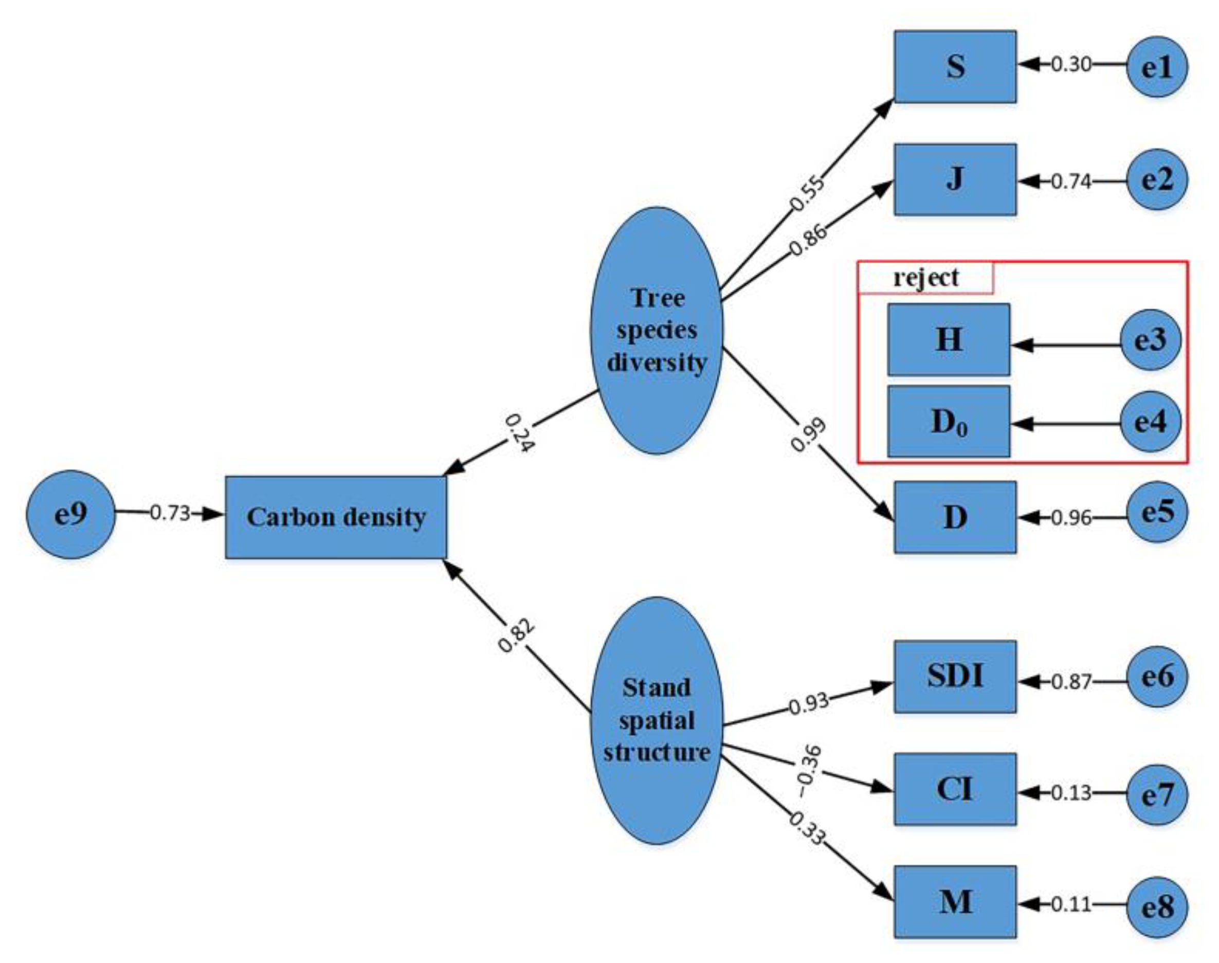
3.2. Impacts of Species Diversity and Stand Spatial Structure on Carbon Density

The Pearson correlation between eight indices and carbon density was analyzed. According to the Pearson correlation coefficients ranked in descending order, SDI (0.781 **) > S (0.564 **) > M (0.523 **) > H (0.491 **) > D₀ (0.466 **) > D (0.446 **) > J (0.256 **) > CI (−0.258 **), with all indices showing significant correlations at the 0.01 level. Due to the serious issue of collinearity between D₀ and H, which caused the model to be unstable and poorly fitted, these two factors were removed from the final structural equation modeling (SEM) analysis (Figure 2).

The $x^2/df$ value of the final model is 2.13, with a CFI of 0.927 and an RMSEA of 0.058, indicating that the model is good. Among the two latent variables, the path coefficient of forest spatial structure is as high as 0.82, while the path coefficient of tree species diversity is 0.24. In the forest stand spatial structure indices, SDI has the highest path coefficient of 0.93, followed by M with a path coefficient of 0.33, and CI with a path coefficient of −0.36, which is mainly due to the high competition intensity among tree species in the study area. In the tree species diversity indices, D has the highest path coefficient of 0.99, followed by J (0.86) and S (0.55).

3.3. Carbon Density Prediction Based on Tree Species Diversity and Stand Spatial Structure Indices

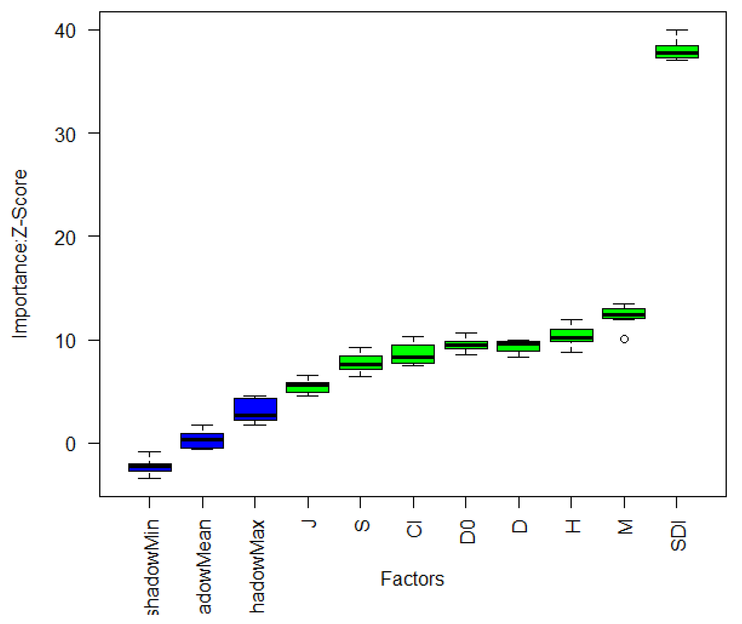
3.3.1. Feature Factor Selection

Boruta variable selection method determines the importance of each feature by comparing its importance with that of randomly generated “shadow features”. The results of Boruta variable selection indicate eight factors were considered to have a significant impact on the target variable (Figure 3). The results can serve as a basis for feature selection to build simpler and more interpretable models.

Based on the variable screening results, it can be concluded that all eight factors exhibit a strong correlation with forest carbon density. Among them, the importance of SDI is significantly higher than that of the other factors. The higher the density of forest stands, the stronger the photosynthesis and carbon fixation capacity of the forest stands. However, when the density of forest stands is too high, the trees will compete for limited light and nutrients, which can have a negative impact on carbon fixation [51]. The CI of forest stands reflects the intensity of competition between tree species within the forest stand. A higher competition index indicates more intense competition between tree species, which affects their access to resources and growing space, ultimately affecting the carbon fixation capacity of the forest stands [52]. A higher degree of mixing of tree species (M) within forest stands results in greater species richness, allowing for better utilization of the ecological niche differences between different tree species, and more efficient utilization of spatial resources within the forest stands, leading to a more stable forest ecosystem and an increase in carbon fixation capacity [53]. Different tree species have different nutrient absorption and production capabilities, and an increase in tree species richness (S) can enhance the overall nutrient absorption capacity, thus promoting forest growth and carbon sequestration. Improving tree species evenness (J) can create a more balanced competition environment for different tree species in a forest stand, thereby promoting the overall forest growth rate and carbon sequestration [54]. An increase in tree species diversity (H, D and D₀) can reduce the dependence of the forest stand on a particular tree species and enhance the stability of the whole forest ecosystem [55]. Therefore, improving species richness, evenness and diversity can enhance the health and stability of the forest ecosystem, thereby improving the forest growth and carbon fixation capacity.

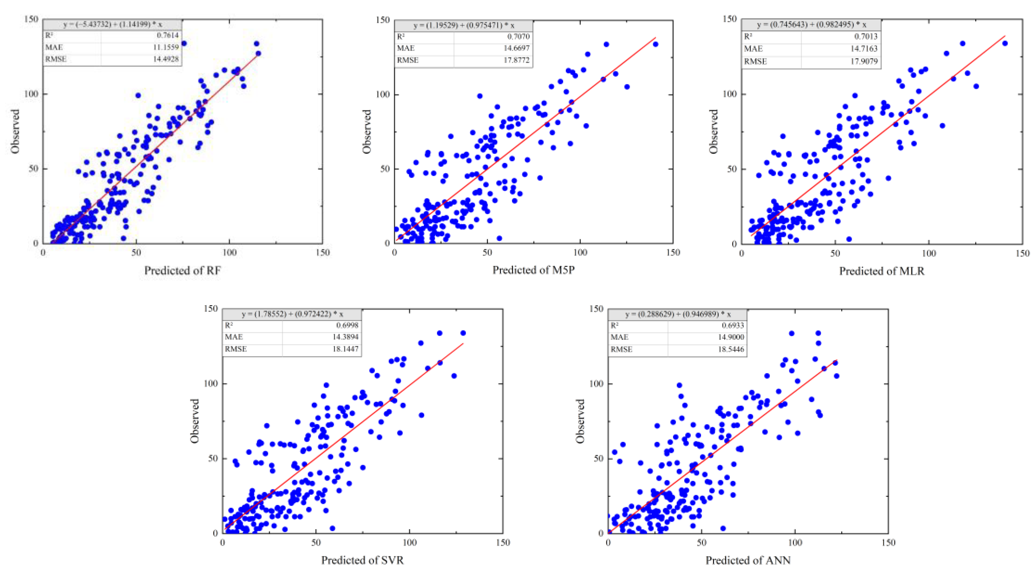
3.3.2. Model Accuracy Evaluation

The six indices were added into the RF, MLR, M5P, ANN and SVR models, respectively, to establish the forest carbon density estimation model, which was verified using 10-fold cross validation. The model accuracy evaluation results are shown in Figure 4.

Among the five estimation models, the prediction accuracy of RF is the highest (R² = 0.7614), followed by M5P (R² = 0.7070), MLR (R² = 0.7013), SVR (R² = 0.6998) and ANN (R² = 0.6933). The predictive performances of the M5P, MLR, SVR and ANN models exhibit minimal differences, while the RF model outperforms the other models in terms of prediction accuracy. When RF model is built, the model uses unbiased training data. The larger the training set of the RF model, the better the model can capture patterns and correlations in the data, resulting in increased accuracy and generalization capability of the model. M5P can capture non-linear relationships between input and output variables, making M5P more flexible in modeling complex data. M5P provides an interpretable model in the form of decision trees, which can help in understanding the relationship between input and output variables. On the other hand, M5P provides a mathematical formula that may be difficult to interpret. Overall, the M5P model is more flexible, efficient and interpretable than the MLR model, so the prediction accuracy is higher. The performance of ANN model may be limited by variables and data volume in this paper, and its accuracy is lowest.

3.3.3. Carbon Density Estimation Based on RF Model

As shown in Figure 5, the mean forest carbon density estimated by RF is 43.176 tC/ha. The regions with higher carbon density are primarily located in the central and southern areas with higher elevations, while lower-density forests are mainly distributed in the western and northeastern regions with lower elevations in hilly river valleys. The mountainous regions with higher elevations have lower population densities and higher forest cover rate, resulting in higher carbon density. In contrast, the hilly river valleys with lower elevations have higher population densities, lower forest cover and greater human interference, leading to poor forest quality. Thus, the spatial distribution of carbon density aligns with the topographical and socio-economic conditions of the study area.

The Guangdong province has divided its forest management plan into seven primary zones, with the northwestern region of Shaoguan falling under zone NO. 1 and the southeastern region falling under zone NO. 2. A statistical study was conducted to compare the forest carbon densities between these two management zones (

Table 3. Statistics of carbon density by forest management sub-region in Shaoguan.

Zone	Forest Management Sub-Region	Mean (tC/ha)	Min (tC/ha)	Max (tC/ha)	SD (tC/ha)
NO. 1	Evergreen Broad-leaved and Coniferous Broad-leaved Mixed Forest Management Sub-region	40.004	4.654	109.069	25.058
NO. 2	Water Conservation Forest and General Timber Forest Management Sub-region	43.178	4.453	109.650	25.419

). The mean forest carbon density of the NO. 2 is the higher, with 43.178 tC/ha. This is mainly related to high altitude, inconvenient traffic, less human disturbance, high forest coverage and a high proportion of public welfare forests. The mean forest carbon density of the NO. 1 is 40.004 tC/ha. The forest coverage in this sub-region is high, but the proportion of young and middle-aged forests is high, leading to lower forest carbon density.

3.4. Suggestions on Management Measures to Improve Forest Carbon Density

Forest carbon density of different forest types based on RF model data is shown in

Table 4. Carbon density of different forest types.

Forest Type	Carbon Density (tC/ha)				Percentage of Sample Plots (%)
	Min	Max	Mean	SD
Coniferous pure forest	2.312	133.896	24.047	19.623	29.677
Broad-leaved pure forest	1.430	64.539	28.879	22.262	8.387
Coniferous mixed forest	17.495	74.512	42.454	20.555	3.226
Broad-leaved mixed forest	45.500	133.762	77.414	20.883	47.097
Coniferous and Broad-leaved mixed forest	14.415	81.303	36.492	22.410	11.613

. The results showed that the ranking of forest types based on carbon density, from highest to lowest, was as follows: broad-leaved mixed forest (77.414 tC/ha), coniferous mixed forest (42.454 tC/ha), coniferous and broad-leaved mixed forest (36.492 tC/ha), broad-leaved pure forest (28.879 tC/ha) and coniferous pure forest (24.047 tC/ha). According to the proportion of different forest types in the total forest sample plots, the broad-leaved mixed forest is the highest. The carbon fixing capacity of Coniferous pure forest is the lowest, but the proportion of sample plots is the second.

Forest carbon density of different age groups based on RF model data is shown in

Table 5. Carbon density of different age groups [27].

Age Group	Carbon Density (tC/ha)				Percentage of Sample Plots (%)
	Min	Max	Mean	SD
Young forest	2.313	83.781	33.459	22.877	44.118
Middle aged forest	4.402	116.629	56.235	33.636	44.117
Near-mature forest	21.5436	79.006	57.399	35.082	8.824
Mature forest	25.227	133.762	73.915	38.737	1.765
Over-mature forest	9.675	133.896	69.325	50.771	1.176

. The carbon density of young and middle-aged forests is low in different age groups. According to the proportion of different age groups in the total forest sample plots, the young and middle-aged forest is up to 88.235%. The carbon fixing capacity of mature forest is the highest, but the proportion of sample plots is less than 2%.

It can be seen from Table 4 that although Shaoguan city has increased the proportion of planting area of broad-leaved mixed forests in recent years, the high proportion of pure coniferous forest in the forest indicates an urgent need for continued efforts to increase the percentage of regeneration area with mixed tree species. It can be seen from Table 5 that the age structure of forest stands in Shaoguan city is seriously unbalanced, and the age group structure need to be adjusted.

Since the carbon density of broad-leaved mixed forest is much higher than that of coniferous pure forest and broad-leaved pure forest, two or more tree species should be selected for afforestation to increase the proportion of mixed forest. The forest age class structure in the study is irrational, and the proportion of young and middle-aged forests with low unit stock volume is large. Therefore, the forest carbon density can be increased by extending the harvesting age of the timber forests to increase the proportion of near-mature and mature forests. Forest protection should be further strengthened to prevent human disturbances such as illegal cutting and conversion of forest land to farms and buildings. When harvesting trees, selective cutting and shelter wood cutting methods instead of clear cutting should be selected to keep forest land with vegetation coverage and increases species diversity. When clear cutting is necessary, the logging residues should be retained on the cutting site to prevent degradation of forest land.

4. Discussion

The NFCI data of Shaoguan city in 2017 were used to calculate five species diversity indices which include Patrick index, Shannon index, Simpson index, Inverse Simpson index, Pielou’s Evenness index, and three stand spatial structure indices including Reineke’s stand density index, Hegyi’s competition index and Simple mingling degree. Five models of RF, MRL, M5P, SVR and ANN, were established to estimate the forest carbon density. The purpose of this paper is exploring a new approach to carbon intensity prediction based on commonly used species diversity indices and stand spatial structure indices. The analysis results of relationship between the species diversity index, stand spatial structure indices and carbon density, together with the analysis on the causes of carbon density differences in different management sub-regions, can provide a scientific basis for the formulation of forest management measures to increase forest carbon sinks and reduce emissions.

The results of this paper show that there is a significant difference in the carbon density of different forest types or age groups in Shaoguan city. The forest carbon density (77.414 tC/ha) and the proportion (47.097%) of sample plots of broad-leaved mixed forest are the highest. The carbon density of coniferous pure forest (24.047 tC/ha) is the lowest, but the proportion of sample plots of this type of forest (29.677%) is the second highest. It can be seen that although the adjustment of forest types in Shaoguan city has achieved initial results in recent years, there is still room for further improvement. The forest carbon density of young and middle-aged forest is lower, but the proportion of sample plots of these two kinds of forest types is as high as 88.235%, indicating that there is an imbalance in the age structure of Shaoguan City. In this paper, five machine learning models which were used to predict forest carbon density based on eight indices have higher precision with R² above 0.690. The accuracy of RF model is the highest, with R² of 0.7614. The average forest carbon density based on the optimal prediction model of RF in Shaoguan is 43.176 tC/ha, which is higher than the forest carbon density of Guangdong Province (32.200 tC/ha) [56]. The forest carbon density of Shaoguan city is higher than that of other surrounding areas, such as Hunan Province (25.000 tC/ha) [57], and is slightly higher than other regions at the same latitude, such as Guangxi Province (42.340 tC/ha) [58]. The average forest carbon density in China is 43.95 tC/ha [59], and Shaoguan city is slightly below the average. The average carbon density of forests in the United States and Russia is 61.000 tC/ha and 36.000 tC/ha [60], respectively. Shaoguan city is higher than Russia, but lower than the United States. The subtropical forests carbon density of dominant forest stands varied from 107.930 to 274.150 t/Cha in Central Himalaya [61]. Total carbon stock in the forests of the Khyber Pakhtunkhwa province of Pakistan was estimated with an average of 127.660 +/− 9.320 tC/ha [62]. The carbon density of subtropical forests in South America was measures at 123.250 tC/ha [63]. It is worth mentioning that the carbon density of subtropical forests in these countries or regions is two to three times that of the study area.

Since species diversity and stand spatial structure affects tree photosynthesis, soil fertility and water status, and is significantly related to tree DBH and height, using species diversity indices and stand spatial structure to estimate forest carbon density could be a feasible method with higher accuracy. However, forest structure is complex, and forest carbon density is influenced by both spatial and non-spatial structures. This paper only used five species diversity indices and three stand spatial structure indices to predict forest carbon density without considering the effect of forest non-spatial structure. Therefore, the prediction results may be affected to some extent. The prediction of forest carbon density based on biodiversity index, spatial structure index and non-spatial structure index will be the direction of our further research.

5. Conclusions

Forest carbon density is strongly influenced by forest types, age structure, site conditions and management levels, which can be reflected by the tree species diversity index and stand spatial structure indices. By using the tree species diversity index, stand spatial structure and machine learning models, it is possible to accurately predict forest carbon density, as well as to quickly obtain the distribution maps of forest carbon storage in the study area. In addition, the analysis on relationship between the species diversity index, stand spatial structure and carbon density, and the carbon density differences in forests of different types and age classes can provide a scientific basis for the making of strategies to increase carbon sink and reduce emissions. The method proposed in this paper can be extended to other subtropical regions of China for efficient prediction and analysis of forest carbon density.

References

1. Winkler, H. Climate change and developing countries. S. Afr. J. Sci. 2005, 101, 355–364. [Google Scholar]
2. Kikstra, J.S.; Nicholls, Z.R.J.; Smith, C.J.; Lewis, J.; Lamboll, R.D.; Byers, E.; Sandstad, M.; Meinshausen, M.; Gidden, M.J.; Rogelj, J.; et al. The IPCC Sixth Assessment Report WGIII climate assessment of mitigation pathways: From emissions to global temperatures. Geosci. Model Dev. 2022, 15, 9075–9109. [Google Scholar] [CrossRef]
3. Stocker. Climate Change 2013; Cambridge University Press: Cambridge, UK, 2014. [Google Scholar]
4. Kramer, P.J. Carbon Dioxide Concentration, Photosynthesis, and Dry Matter Production. Bioscience 1981, 31, 29–33. [Google Scholar] [CrossRef]
5. Zedaker, S.M. Forest ecosystems: Concepts and management. For. Sci. 1986, 3, 841–842. [Google Scholar] [CrossRef]
6. Dixon, R.K.; Solomon, A.M.; Brown, S.; Houghton, R.A.; Trexier, M.C.; Wisniewski, J. Carbon Pools and Flux of Global Forest Ecosystems. Science 1994, 263, 185–190. [Google Scholar] [CrossRef] [PubMed]
7. Kurz, W.A.; Apps, M.J. Contribution of Northern Forests to the Global C Cycle: Canada as a Case Study; Springer: Dordrecht, The Netherlands, 1993; pp. 163–176. [Google Scholar] [CrossRef]
8. Mi, X.C.; Feng, G.; Zhang, J.; Hu, Y.; Zhu, L.; Ma, K. Review on biodiversity science in China. Bull. Chin. Acad. Sci. 2021, 36, 384–398. [Google Scholar] [CrossRef]
9. Liang, J.; Crowther, T.W.; Picard, N.; Wiser, S.; Zhou, M.; Alberti, G.; Schulze, E.-D.; McGuire, A.D.; Bozzato, F.; Pretzsch, H.; et al. Positive biodiversity-productivity relationship predominant in global forests. Science 2016, 354, aaf8957. [Google Scholar] [CrossRef]
10. Yin, L.; Bao, W.; Bongers, F.; Chen, B.; Chen, G.; Guo, K.; Jiang, M.; Lai, J.; Lin, D.; Liu, C.; et al. Drivers of tree carbon storage in subtropical forests. Sci. Total Environ. 2019, 654, 684–693. [Google Scholar]
11. Huang, Y.; Chen, Y.; Castro-Izaguirre, N.; Baruffol, M.; Brezzi, M.; Lang, A.; Li, Y.; Härdtle, W.; Von Oheimb, G.; Yang, X.; et al. Impacts of species richness on productivity in a large-scale subtropical forest experiment. Science 2018, 362, 80–83. [Google Scholar] [CrossRef]
12. Van Con, T.; Thang, N.T.; Ha, D.T.T.; Khiem, C.C.; Quy, T.H.; Lam, V.T.; Van Do, T.; Sato, T. Relationship between aboveground biomass and measures of structure and species diversity in tropical forests of Vietnam. For. Ecol. Manag. 2013, 310, 213–218. [Google Scholar] [CrossRef]
13. Vance-Chalcraft, H.D.; Willig, M.R.; Cox, S.B.; Lugo, A.E.; Scatena, F.N. Relationship Between Aboveground Biomass and Multiple Measures of Biodiversity in Subtropical Forest of Puerto Rico. Biotropica 2009, 42, 290–299. [Google Scholar] [CrossRef]
14. Shahid, M.; Joshi, S.P. Relationship between Tree Species Diversity and Carbon Stock Density in Moist Deciduous Forest of Western Himalayas, India. J. For. Environ. Sci. 2017, 33, 39–48. [Google Scholar] [CrossRef]
15. Kumar, B.M. Species richness and aboveground carbon stocks in the homegardens of central Kerala, India. Agric. Ecosyst. Environ. 2011, 140, 430–440. [Google Scholar] [CrossRef]
16. Liu, X.; Trogisch, S.; He, J.-S.; Niklaus, P.; Bruelheide, H.; Tang, Z.; Erfmeier, A.; Scherer-Lorenzen, M.; Pietsch, K.A.; Yang, B.; et al. Tree species richness increases ecosystem carbon storage in subtropical forests. Proc. R. Soc. B Boil. Sci. 2018, 285, 20181240. [Google Scholar] [CrossRef]
17. Yang, S.; Zou, W.; Yin, G.; Li, R.S.; Yang, J.C. Species diversity and influencing factors of artificial forest communities in Shunde. Guangdong. Ecol. Sci. 2010, 29, 427–431. [Google Scholar]
18. Hall, R.; Skakun, R.; Arsenault, E.; Case, B. Modeling forest stand structure attributes using Landsat ETM+ data: Application to mapping of aboveground biomass and stand volume. For. Ecol. Manag. 2006, 225, 378–390. [Google Scholar] [CrossRef]
19. Zheng, G.; Chen, J.M.; Tian, Q.J.; Ju, W.M.; Xia, X.Q. Combining remote sensing imagery and forest age inventory for biomass mapping. J. Environ. Manag. 2007, 85, 616–623. [Google Scholar] [CrossRef]
20. Ou, G.L.; Li, C.; Lv, Y.Y.; Wei, A.C.; Xiong, H.X.; Xu, H.; Wang, G.X. Improving aboveground biomass estimation of Pinus densata forests in Yunnan using Landsat 8 Imagery by incorporating age dummy variable and method comparison. Remote Sens. 2019, 11, 738. [Google Scholar] [CrossRef]
21. Li, Z.; Huang, H.; Zhang, Y.; Meng, Y. Subtropical evergreen broad-leaved forest: The most diverse subtropical forest in the world. For. Hum. 2022, 008, 66–71. [Google Scholar]
22. Xie, X.; Wang, Q.; Dai, L.; Su, D.; Wang, X.; Qi, G.; Ye, Y. Application of China’s National Forest Continuous Inventory Database. Environ. Manag. 2011, 48, 1095–1106. [Google Scholar] [CrossRef]
23. Zeng, W. Establishment of a univariate tree biomass model for 34 tree species based on wood density. For. Resour. Manag. 2017, 6, 41–46. [Google Scholar] [CrossRef]
24. Zhang, H. Measurement and analysis of carbon content rates of eight tree species in Guangdong province. For. Resour. Manag. 2018, 1, 148–154. [Google Scholar]
25. Solow, A.R.; Polasky, S. Measuring biological diversity. Environ. Ecol. Stat. 1994, 1, 95–103. [Google Scholar] [CrossRef]
26. Jost, L. Entropy and diversity. Oikos 2006, 113, 363–375. [Google Scholar] [CrossRef]
27. GB/T 38590-2020; Technical Regulations for Continuous Forest Inventory. The National Forestry and Grassland Administration: Beijing, China, 2020.
28. Vanderschaaf, C.L. Reineke’s stand density index: A quantitative and non-unitless measure of stand density. In Proceedings of the 15th Biennial Southern Silvicultural Research Conference, Hot Springs, AR, USA, 17–20 November 2008; U.S. Department of Agriculture, Forest Service, Southern Research Station: Asheville, NC, USA, 2013. [Google Scholar]
29. Marchi, M. Nonlinear versus linearised model on stand density model fitting and stand density index calculation: Analysis of coefficients estimation via simulation. J. For. Res. 2019, 30, 1595–1602. [Google Scholar] [CrossRef]
30. Sandoval, S.; Cancino, J. Modeling the edge effect in even-aged Monterrey pine (Pinus radiata D. Don) stands incorporating a competition index. For. Ecol. Manag. 2008, 256, 78–87. [Google Scholar] [CrossRef]
31. Hu, Y.B.; Hui, G.Y. A new method for measuring population distribution patterns of forest trees based on the mingling degree. J. Beijing For. Univ. 2015, 37, 9–21. [Google Scholar] [CrossRef]
32. Hoyle, R.H. Introduction to the special section: Structural equation modeling in clinical research. J. Consult. Clin. Psychol. 1994, 62, 427–428. [Google Scholar] [CrossRef]
33. Wen, Z.L.; Kittai, H.; Marsh, H.W. Structural equation model: Cutoff criteria for goodness of fit indices and chi-square test. Acta Psychol. Sin. 2004, 36, 186–194. [Google Scholar]
34. Chen, H.; Qin, Z.; Zhai, D.-L.; Ou, G.; Li, X.; Zhao, G.; Fan, J.; Zhao, C.; Xu, H. Mapping Forest Aboveground Biomass with MODIS and Fengyun-3C VIRR Imageries in Yunnan Province, Southwest China Using Linear Regression, K-Nearest Neighbor and Random Forest. Remote Sens. 2022, 14, 5456. [Google Scholar] [CrossRef]
35. He, J.; Fan, C.; Geng, Y.; Zhang, C.; Zhao, X.; von Gadow, K. Assessing scale-dependent effects on Forest biomass productivity based on machine learning. Ecol. Evol. 2022, 12, e9110. [Google Scholar] [CrossRef]
36. Li, C.; Li, M.; Li, Y.; Qian, P. Estimating aboveground forest carbon density using Landsat 8 and field-based data: A comparison of modelling approaches. Int. J. Remote Sens. 2020, 41, 4269–4292. [Google Scholar] [CrossRef]
37. Liu, Y. Mathematical model of multiple linear regression. J. Shenyang Inst. Eng. 2005, 1, 128–129. [Google Scholar]
38. Ross, J. Quinlan: Learning with continuous classes. In Proceedings of the 5th Australian Joint Conference on Artificial Intelligence, Hobart, Tasmania, 16–18 November 1992; World Scientific: Singapore, 1992; pp. 343–348. [Google Scholar]
39. Breiman, L. Random forests. Mach. Learn. 2001, 45, 5–32. [Google Scholar] [CrossRef]
40. Li, T.; Li, M.; Ren, F.; Tian, L. Estimation and Spatio-Temporal Change Analysis of NPP in Subtropical Forests: A Case Study of Shaoguan, Guangdong, China. Remote Sens. 2022, 14, 2541. [Google Scholar] [CrossRef]
41. Pavlov, Y.L. Limit distributions of the height of a random forest of plane rooted trees. Discret. Math. Appl. 1994, 4, 73–88. [Google Scholar] [CrossRef]
42. Safitri, L.; Mardiyati, S.; Rahim, H. Forecasting the mortality rates of Indonesian population by using neural network. J. Phys. Conf. Ser. 2018, 974, 012030. [Google Scholar] [CrossRef]
43. Xiao, F. Forest Coverage Prediction Based on Least Squares Support Vector Regression Algorithm. Adv. Mater. Res. 2012, 446–449, 2978–2982. [Google Scholar] [CrossRef]
44. Kursa, M.B.; Rudnicki, W.R. Feature Selection with theBorutaPackage. J. Stat. Softw. 2010, 36, 1–13. [Google Scholar] [CrossRef]
45. Singh, G.; Panda, R.K. Daily Sediment Yield Modeling with Artificial Neural Network Using 10-fold Cross Validation Method: A Small Agricultural Watershed, Kapgari, India. Int. J. Earth Sci. Eng. 2010, 4, 443–450. [Google Scholar]
46. Zheng, B.; Agresti, A. Summarizing the predictive power of a generalized linear model. Stat. Med. 2000, 19, 1771–1781. [Google Scholar] [CrossRef]
47. Zimmerman, D.; Pavlik, C.; Ruggles, A.; Armstrong, M. An Experimental Comparison of Ordinary and Universal Kriging and Inverse Distance Weighting. J. Int. Assoc. Math. Geol. 1999, 31, 375–390. [Google Scholar] [CrossRef]
48. Myers, D.E. Matrix formulation of co-kriging. J. Int. Assoc. Math. Geol. 1982, 14, 249–257. [Google Scholar] [CrossRef]
49. Goovaerts, P. Geostatistical approaches for incorporating elevation into the spatial interpolation of rainfall. J. Hydrol. 2000, 228, 113–129. [Google Scholar] [CrossRef]
50. Jiao, W.; Wang, W.; Peng, C.; Lei, X.; Ruan, H.; Li, H.; Yang, Y.; Grabarnik, P.; Shanin, V. Improving a Process-Based Model to Simulate Forest Carbon Allocation under Varied Stand Density. Forests 2022, 13, 1212. [Google Scholar] [CrossRef]
51. Cai, H.; Di, X.; Chang, S.X.; Jin, G. Stand density and species richness affect carbon storage and net primary productivity in early and late successional temperate forests differently. Ecol. Res. 2016, 31, 525–533. [Google Scholar] [CrossRef]
52. Wu, C.; Chen, D.; Sun, X.; Zhang, S. Contributions of competition on Larix kaempferi tree-ring growth were higher than long-term climate in China. Agric. For. Meteorol. 2022, 320, 108967. [Google Scholar] [CrossRef]
53. Hulvey, K.B.; Hobbs, R.J.; Standish, R.J.; Lindenmayer, D.B.; Lach, L.; Perring, M.P. Benefits of tree mixes in carbon plantings. Nat. Clim. Chang. 2013, 3, 869–874. [Google Scholar] [CrossRef]
54. Shirima, D.D.; Totland, Ø.; Munishi, P.K.; Moe, S.R. Relationships between tree species richness, evenness and aboveground carbon storage in montane forests and miombo woodlands of Tanzania. Basic Appl. Ecol. 2015, 16, 239–249. [Google Scholar] [CrossRef]
55. Ruiz-Jaen, M.C.; Potvin, C. Tree Diversity Explains Variation in Ecosystem Function in a Neotropical Forest in Panama. Biotropica 2010, 42, 638–646. [Google Scholar] [CrossRef]
56. Shao, Y.; Zhong, B.; Yang, Z.; Fan, J.; Lu, G.; Xue, L. Distribution of forest resources and carbon storage in Guangdong Province. Hunan For. Sci. Technol. 2013, 40, 34–38. [Google Scholar]
57. Chen, L.-C.; Guan, X.; Li, H.-M.; Wang, Q.-K.; Zhang, W.-D.; Yang, Q.-P.; Wang, S.-L. Spatiotemporal patterns of carbon storage in forest ecosystems in Hunan Province, China. For. Ecol. Manag. 2018, 432, 656–666. [Google Scholar] [CrossRef]
58. Li, H.; Wang, X.; Meng, J. Research on the dynamic changes of carbon storage at the level of forest management units: A case study of the Hotan Center in Guangxi. J. Zhejiang For. Sci. Technol. 2019, 39, 29–35. [Google Scholar]
59. Zhao, M.; Yang, J.; Zhao, N.; Xiao, X.; Yue, T.; Wilson, J.P. Estimation of the relative contributions of forest areal expansion and growth to China’s forest stand biomass carbon sequestration from 1977 to 2018. J. Environ. Manag. 2021, 300, 113757. [Google Scholar] [CrossRef] [PubMed]
60. Wang, X.; Feng, Z.; Ouyang, Z. Vegetation carbon storage and density of forest ecosystems in China. Ying Yong Sheng Tai Xue Bao 2001, 12, 13–16. [Google Scholar]
61. Joshi, V.C.; Negi, V.S.; Bisht, D.; Sundriyal, R.; Arya, D. Tree biomass and carbon stock assessment of subtropical and temperate forests in the Central Himalaya, India. Trees For. People 2021, 6, 100147. [Google Scholar] [CrossRef]
62. Ali, A.; Ashraf, M.I.; Gulzar, S.; Akmal, M. Estimation of forest carbon stocks in temperate and subtropical mountain systems of Pakistan: Implications for REDD+ and climate change mitigation. Environ. Monit. Assess. 2020, 192, 198. [Google Scholar] [CrossRef]
63. Bordin, K.M.; Esquivel-Muelbert, A.; Bergamin, R.S.; Klipel, J.; Picolotto, R.C.; Frangipani, M.A.; Zanini, K.J.; Cianciaruso, M.V.; Jarenkow, J.A.; Jurinitz, C.F.; et al. Climate and large-sized trees, but not diversity, drive above-ground biomass in subtropical forests. For. Ecol. Manag. 2021, 490, 119126. [Google Scholar] [CrossRef]
Figure 1. Location and elevation of the study area.
Forests 14 01105 g001
Figure 2. Standardization path of SEM for eight stand indices and carbon density.
Forests 14 01105 g002
Figure 3. Boruta result plot eight indices. Blue boxplots correspond to minimal, average and maximum Z score of a shadow attribute. Green boxplots represent Z scores of confirmed attributes.
Forests 14 01105 g003
Figure 4. Accuracy evaluation of five estimation models. The blue circle represents the forest carbon density, and the line represents the fitting line between the observed and predicted values.
Forests 14 01105 g004
Figure 5. Distribution map of forest carbon density based on RF model.
Forests 14 01105 g005