
Review of Remote Sensing-Based Methods for Forest Aboveground Biomass Estimation: Progress, Challenges, and Prospects

 ,
,  ,
,
Abstract
1. Introduction
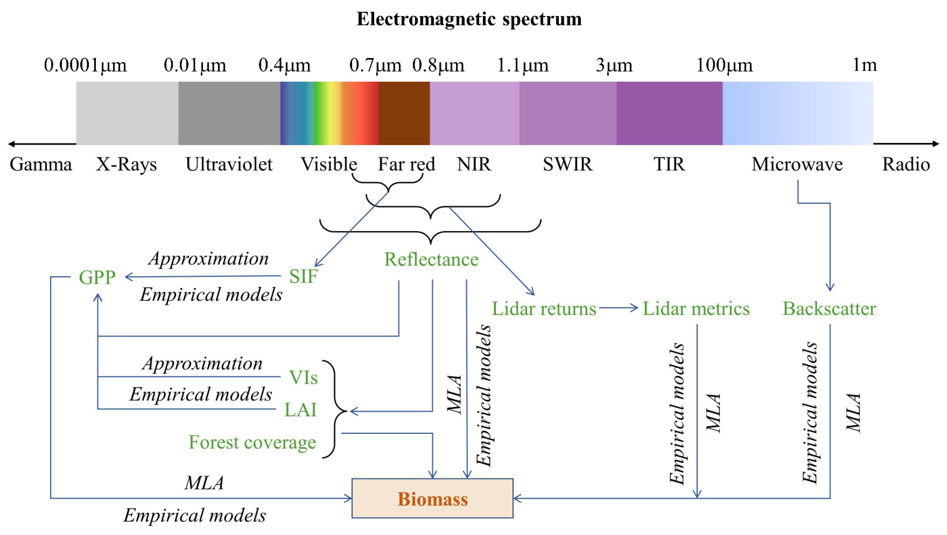
2. Principles of AGB Estimation via Remote Sensing
3. Remote Sensing Procedures in Forest AGB Estimation
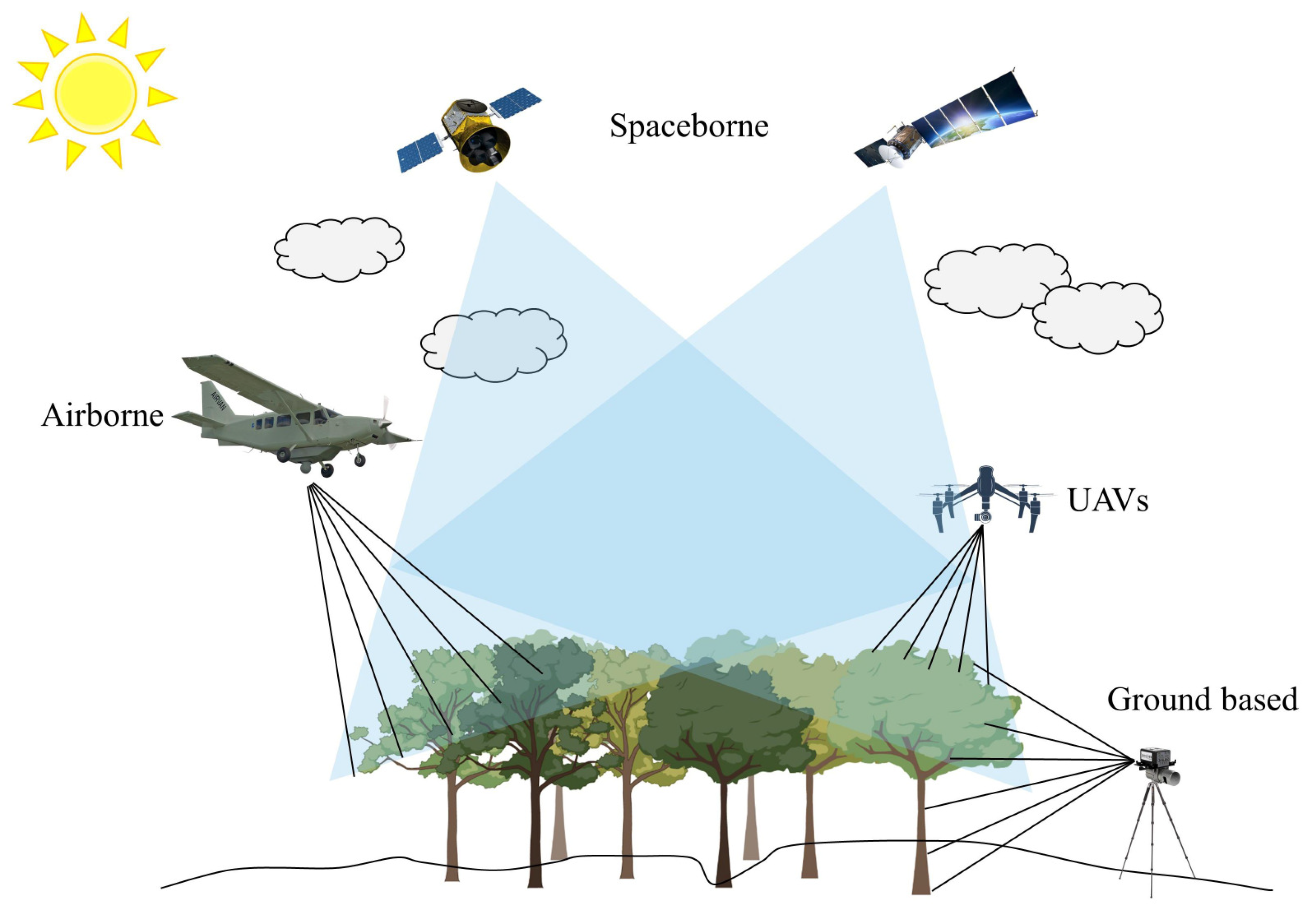
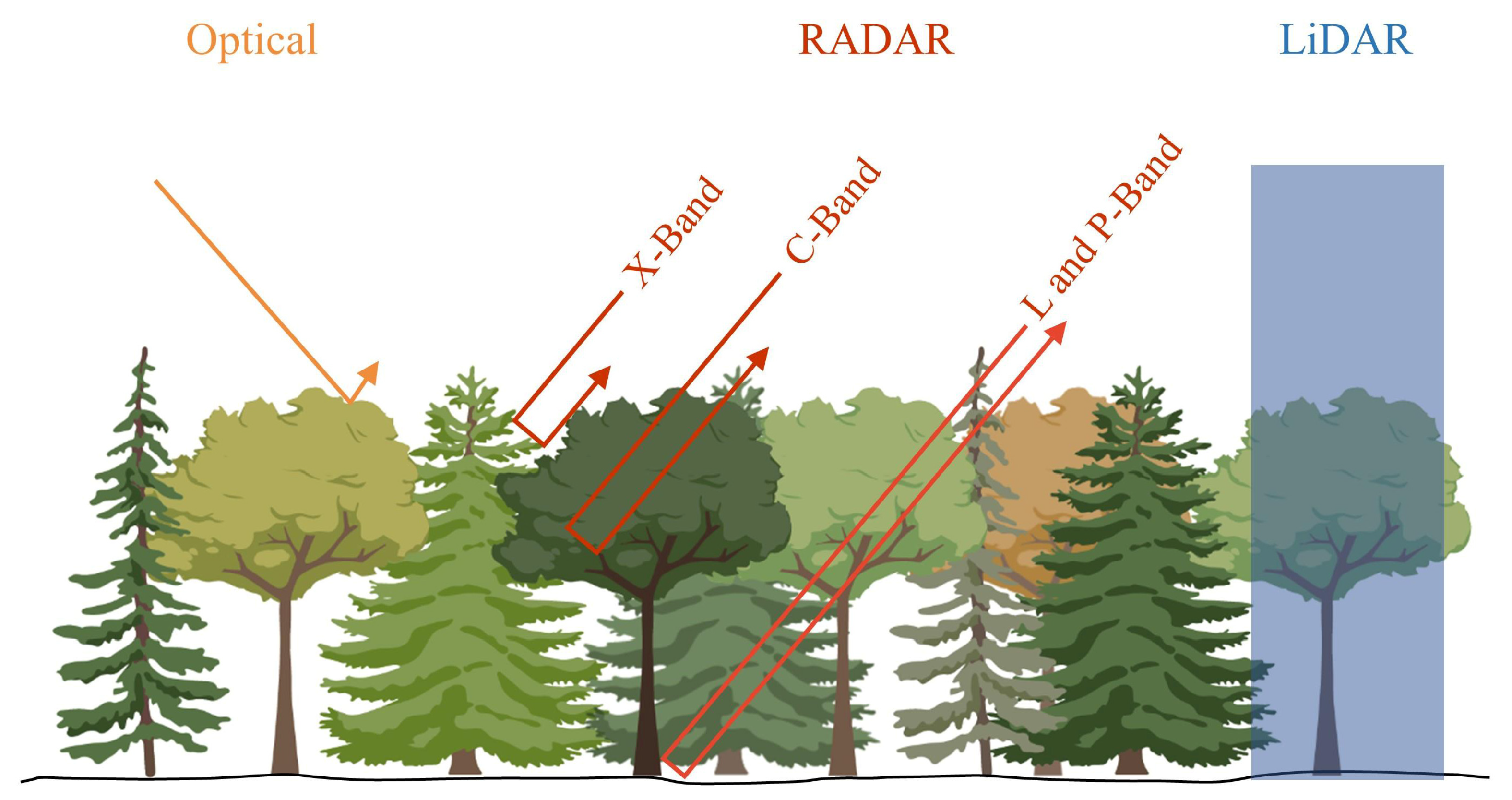
3.1. Remotely Sensed Data Sources
3.1.1. Passive Optical Remote Sensing of AGB
3.1.2. Microwave Remote Sensing of AGB
3.1.3. LiDAR Remote Sensing of AGB
3.1.4. Multi-Source Remote Sensing of AGB
3.2. AGB Estimation Methods
3.2.1. Empirical Modeling
3.2.2. Physical Modeling
3.2.3. Mechanistic Modeling
3.2.4. Comprehensive Modeling
4. Uncertainty in Remote Sensing Estimation of Forest AGB
5. Prospects for Remote Sensing of Forest AGB Estimation
6. Conclusions
Author Contributions
Funding
Acknowledgments
Conflicts of Interest
Abbreviations
References
- Nerem, R.S.; Beckley, B.D.; Fasullo, J.T.; Hamlington, B.D.; Masters, D.; Mitchum, G.T. Climate-change-driven accelerated sea-level rise detected in the altimeter era. Proc. Natl. Acad. Sci. USA 2018, 115, 2022–2025. [Google Scholar] [CrossRef] [PubMed]
- Radic, V.; Bliss, A.; Beedlow, A.C.; Hock, R.; Miles, E.; Cogley, J.G. Regional and global projections of twenty-first century glacier mass changes in response to climate scenarios from global climate models. Clim. Dynam. 2014, 42, 37–58. [Google Scholar] [CrossRef]
- Zheng, G.X.; Allen, S.K.; Bao, A.; Ballesteros-Canovas, J.A.; Huss, M.; Zhang, G.Q.; Li, J.L.; Yuan, Y.; Jiang, L.L.; Yu, T.; et al. Increasing risk of glacial lake outburst floods from future Third Pole deglaciation. Nat. Clim. Change 2021, 11, 411–417. [Google Scholar] [CrossRef]
- Kang, S.C.; Zhang, Q.G.; Qian, Y.; Ji, Z.M.; Li, C.L.; Cong, Z.Y.; Zhang, Y.L.; Guo, J.M.; Du, W.T.; Huang, J.; et al. Linking atmospheric pollution to cryospheric change in the Third Pole region: Current progress and future prospects. Natl. Sci. Rev. 2019, 6, 796–809. [Google Scholar] [CrossRef]
- Yin, J.B.; Gentine, P.; Zhou, S.; Sullivan, S.C.; Wang, R.; Zhang, Y.; Guo, S.L. Large increase in global storm runoff extremes driven by climate and anthropogenic changes. Nat. Commun. 2018, 9, 4389. [Google Scholar] [CrossRef]
- Ebi, K.L.; Vanos, J.; Baldwin, J.W.; Bell, J.E.; Hondula, D.M.; Errett, N.A.; Hayes, K.; Reid, C.E.; Saha, S.; Spector, J.; et al. Extreme Weather and Climate Change: Population Health and Health System Implications. In Annual Review of Public Health; Fielding, J.E., Ed.; Annual Review of Public Health: San Mateo, CA, USA, 2021; Volume 42, pp. 293–315. [Google Scholar] [CrossRef]
- Hasegawa, T.; Fujimori, S.; Havlik, P.; Valin, H.; Bodirsky, B.L.; Doelman, J.C.; Fellmann, T.; Kyle, P.; Koopman, J.F.L.; Lotze-Campen, H.; et al. Risk of increased food insecurity under stringent global climate change mitigation policy. Nat. Clim. Change 2018, 8, 699–703. [Google Scholar] [CrossRef]
- Bellard, C.; Bertelsmeier, C.; Leadley, P.; Thuiller, W.; Courchamp, F. Impacts of climate change on the future of biodiversity. Ecol. Lett. 2012, 15, 365–377. [Google Scholar] [CrossRef]
- Frumkin, H.; Haines, A. Global Environmental Change and Noncommunicable Disease Risks. In Annual Review of Public Health; Fielding, J.E., Ed.; Annual Review of Public Health: San Mateo, CA, USA, 2019; Volume 40, pp. 261–282. [Google Scholar] [CrossRef]
- Gosling, S.N.; Arnell, N.W. A global assessment of the impact of climate change on water scarcity. Clim. Change 2016, 134, 371–385. [Google Scholar] [CrossRef]
- Hoegh-Guldberg, O.; Jacob, D.; Taylor, M.; Guillen Bolanos, T.; Bindi, M.; Brown, S.; Camilloni, I.; Diedhiou, A.; Djalante, R.; Ebi, K.; et al. The human imperative of stabilizing global climate change at 1.5 °C. Science 2019, 365, 1263. [Google Scholar] [CrossRef]
- Sippel, S.; Meinshausen, N.; Fischer, E.M.; Szekely, E.; Knutti, R. Climate change now detectable from any single day of weather at global scale. Nat. Clim. Change 2020, 10, 35–41. [Google Scholar] [CrossRef]
- Pan, Y.D.; Birdsey, R.A.; Fang, J.Y.; Houghton, R.; Kauppi, P.E.; Kurz, W.A.; Phillips, O.L.; Shvidenko, A.; Lewis, S.L.; Canadell, J.G.; et al. A Large and Persistent Carbon Sink in the World’s Forests. Science 2011, 333, 988–993. [Google Scholar] [CrossRef] [PubMed]
- Houghton, R.A.; Hall, F.; Goetz, S.J. Importance of biomass in the global carbon cycle. J. Geophys. Res.-Biogeosci. 2009, 114, G00E03. [Google Scholar] [CrossRef]
- Molotoks, A.; Stehfest, E.; Doelman, J.; Albanito, F.; Fitton, N.; Dawson, T.P.; Smith, P. Global projections of future cropland expansion to 2050 and direct impacts on biodiversity and carbon storage. Glob. Change Biol. 2018, 24, 5895–5908. [Google Scholar] [CrossRef] [PubMed]
- Tian, L.; Tao, Y.; Fu, W.X.; Li, T.; Ren, F.; Li, M.Y. Dynamic Simulation of Land Use/Cover Change and Assessment of Forest Ecosystem Carbon Storage under Climate Change Scenarios in Guangdong Province, China. Remote Sens. 2022, 14, 2330. [Google Scholar] [CrossRef]
- Payne, N.J.; Cameron, D.A.; Leblanc, J.D.; Morrison, I.K. Carbon storage and net primary productivity in Canadian boreal mixedwood stands. J. For. Res. 2019, 30, 1667–1678. [Google Scholar] [CrossRef]
- Xiao, J.F.; Chevallier, F.; Gomez, C.; Guanter, L.; Hicke, J.A.; Huete, A.R.; Ichii, K.; Ni, W.J.; Pang, Y.; Rahman, A.F.; et al. Remote sensing of the terrestrial carbon cycle: A review of advances over 50 years. Remote Sens. Environ. 2019, 233, 111383. [Google Scholar] [CrossRef]
- Chave, J.; Rejou-Mechain, M.; Burquez, A.; Chidumayo, E.; Colgan, M.S.; Delitti, W.B.; Duque, A.; Eid, T.; Fearnside, P.M.; Goodman, R.C.; et al. Improved allometric models to estimate the aboveground biomass of tropical trees. Glob. Change Biol. 2014, 20, 3177–3190. [Google Scholar] [CrossRef]
- Chang, F.C.; Ko, C.H.; Yang, P.Y.; Chen, K.S.; Chang, K.H. Carbon sequestration and substitution potential of subtropical mountain Sugi plantation forests in central Taiwan. J. Clean. Prod. 2017, 167, 1099–1105. [Google Scholar] [CrossRef]
- Li, D.R.; Wang, C.W.; Hu, Y.M.; Liu, S.G. General Review on Remote Sensing-Based Biomass Estimation. Geomat. Inform. Sci. Wuhan Univ. 2012, 37, 631–635. [Google Scholar] [CrossRef]
- Brown, S.; Sathaye, J.; Cannell, M.; Kauppi, P.E. Mitigation of carbon emissions to the atmosphere by forest management. Commonw. For. Rev. 1996, 75, 80–91. [Google Scholar]
- Lu, D.S.; Batistella, M.; Moran, E. Satellite estimation of aboveground biomass and impacts of forest stand structure. Photogramm. Eng. Remote Sens. 2005, 71, 967–974. [Google Scholar] [CrossRef]
- Zhang, Z.; Tian, X.; Chen, R.X.; He, Q.S. Review of methods on estimating forest above ground biomass. J. Beijing For. Univ. 2011, 33, 144–150. [Google Scholar] [CrossRef]
- Huang, H.B.; Liu, C.X.; Wang, X.Y.; Zhou, X.L.; Gong, P. Integration of multi-resource remotely sensed data and allometric models for forest aboveground biomass estimation in China. Remote Sens. Environ. 2019, 221, 225–234. [Google Scholar] [CrossRef]
- Myneni, R.B.; Dong, J.; Tucker, C.J.; Kaufmann, R.K.; Kauppi, P.E.; Liski, J.; Zhou, L.; Alexeyev, V.; Hughes, M.K. A large carbon sink in the woody biomass of Northern forests. Proc. Natl. Acad. Sci. USA 2001, 98, 14784–14789. [Google Scholar] [CrossRef] [PubMed]
- Nelson, R.; Gobakken, T.; Naesset, E.; Gregoire, T.G.; Stahl, G.; Holm, S.; Flewelling, J. Lidar sampling—Using an airborne profiler to estimate forest biomass in Hedmark County, Norway. Remote Sens. Environ. 2012, 123, 563–578. [Google Scholar] [CrossRef]
- Houghton, R.A. Aboveground Forest Biomass and the Global Carbon Balance. Glob. Change Biol. 2005, 11, 945–958. [Google Scholar] [CrossRef]
- Li, Y.C.; Li, C.; Li, M.Y.; Liu, Z.Z. Influence of Variable Selection and Forest Type on Forest Aboveground Biomass Estimation Using Machine Learning Algorithms. Forests 2019, 10, 1073. [Google Scholar] [CrossRef]
- Zhang, R.; Zhou, X.H.; Ouyang, Z.T.; Avitabile, V.; Qi, J.G.; Chen, J.Q.; Giannico, V. Estimating aboveground biomass in subtropical forests of China by integrating multisource remote sensing and ground data. Remote Sens. Environ. 2019, 232, 111341. [Google Scholar] [CrossRef]
- Narine, L.L.; Popescu, S.; Neuenschwander, A.; Zhou, T.; Srinivasan, S.; Harbeck, K. Estimating aboveground biomass and forest canopy cover with simulated ICESat-2 data. Remote Sens. Environ. 2019, 224, 1–11. [Google Scholar] [CrossRef]
- Fan, W.Y.; Li, M.Z.; Yang, J.M. Forest Biomass Estimation Models of Remote Sensing in Changbai Mountain Forests. Sci. Silvae Sinicae 2011, 47, 16–20. [Google Scholar] [CrossRef]
- Sarker, M.L.R.; Nichol, J.; Iz, H.B.; Bin Ahmad, B.; Rahman, A.A. Forest Biomass Estimation Using Texture Measurements of High-Resolution Dual-Polarization C-Band SAR Data. IEEE Trans. Geosci. Remote 2013, 51, 3371–3384. [Google Scholar] [CrossRef]
- Ali, A.; Lin, S.L.; He, J.K.; Kong, F.M.; Yu, J.H.; Jiang, H.S. Climate and soils determine aboveground biomass indirectly via species diversity and stand structural complexity in tropical forests. For. Ecol. Manag. 2019, 432, 823–831. [Google Scholar] [CrossRef]
- Deng, L.; Liu, S.G.; Kim, D.G.; Peng, C.H.; Sweeney, S.; Shangguan, Z.P. Past and future carbon sequestration benefits of China’s grain for green program. Glob. Environ. Change 2017, 47, 13–20. [Google Scholar] [CrossRef]
- Zhang, Y.Z.; Liang, S.L.; Yang, L. A Review of Regional and Global Gridded Forest Biomass Datasets. Remote Sens. 2019, 11, 2744. [Google Scholar] [CrossRef]
- Cartus, O.; Santoro, M.; Kellndorfer, J. Mapping forest aboveground biomass in the Northeastern United States with ALOS PALSAR dual-polarization L-band. Remote Sens. Environ. 2012, 124, 466–478. [Google Scholar] [CrossRef]
- Ketterings, Q.M.; Coe, R.; van Noordwijk, M.; Ambagau, Y.; Palm, C.A. Reducing uncertainty in the use of allometric biomass equations for predicting above-ground tree biomass in mixed secondary forests. For. Ecol. Manag. 2001, 146, 199–209. [Google Scholar] [CrossRef]
- Kenzo, T.; Furutani, R.; Hattori, D.; Kendawang, J.J.; Tanaka, S.; Sakurai, K.; Ninomiya, I. Allometric equations for accurate estimation of above-ground biomass in logged-over tropical rainforests in Sarawak, Malaysia. J. For. Res. 2009, 14, 365–372. [Google Scholar] [CrossRef]
- Lu, D.S.; Chen, Q.; Wang, G.X.; Liu, L.J.; Li, G.Y.; Moran, E. A survey of remote sensing-based aboveground biomass estimation methods in forest ecosystems. Int. J. Digit. Earth 2016, 9, 63–105. [Google Scholar] [CrossRef]
- Saatchi, S.S.; Houghton, R.A.; Alvala, R.; Soares, J.V.; Yu, Y. Distribution of aboveground live biomass in the Amazon basin. Global Change Biol. 2007, 13, 816–837. [Google Scholar] [CrossRef]
- Baccini, A.; Goetz, S.J.; Walker, W.S.; Laporte, N.T.; Sun, M.; Sulla-Menashe, D.; Hackler, J.; Beck, P.S.A.; Dubayah, R.; Friedl, M.A.; et al. Estimated carbon dioxide emissions from tropical deforestation improved by carbon-density maps. Nat. Clim. Change 2012, 2, 182–185. [Google Scholar] [CrossRef]
- Badreldin, N.; Sanchez-Azofeifa, A. Estimating Forest Biomass Dynamics by Integrating Multi-Temporal Landsat Satellite Images with Ground and Airborne LiDAR Data in the Coal Valley Mine, Alberta, Canada. Remote Sens. 2015, 7, 2832–2849. [Google Scholar] [CrossRef]
- Bouvet, A.; Mermoz, S.; Toan, T.L.; Villard, L.; Mathieu, R.; Naidoo, L.; Asner, G.P. An above-ground biomass map of African savannahs and woodlands at 25 m resolution derived from ALOS PALSAR. Remote Sens. Environ. 2018, 206, 156–173. [Google Scholar] [CrossRef]
- Santoro, M.; Beaudoin, A.; Beer, C.; Cartus, O.; Fransson, J.B.S.; Hall, R.J.; Pathe, C.; Schmullius, C.; Schepaschenko, D.; Shvidenko, A.; et al. Forest growing stock volume of the northern hemisphere: Spatially explicit estimates for 2010 derived from Envisat ASAR. Remote Sens. Environ. 2015, 168, 316–334. [Google Scholar] [CrossRef]
- Tian, X.; Yan, M.; van der Tol, C.; Li, Z.; Su, Z.B.; Chen, E.X.; Li, X.; Li, L.H.; Wang, X.F.; Pan, X.D.; et al. Modeling forest above-ground biomass dynamics using multi-source data and incorporated models: A case study over the qilian mountains. Agric. For. Meteorol. 2017, 246, 1–14. [Google Scholar] [CrossRef]
- Hurtt, G.C.; Fisk, J.; Thomas, R.Q.; Dubayah, R.; Moorcroft, P.R.; Shugart, H.H. Linking models and data on vegetation structure. J. Geophys. Res.-Biogeosci. 2010, 115, G00E10. [Google Scholar] [CrossRef]
- Waring, R.H.; Coops, N.C.; Landsberg, J.J. Improving predictions of forest growth using the 3-PGS model with observations made by remote sensing. For. Ecol. Manag. 2010, 259, 1722–1729. [Google Scholar] [CrossRef]
- Yan, F.; Wu, B.; Wang, Y.J. Estimating spatiotemporal patterns of aboveground biomass using Landsat TM and MODIS images in the Mu Us Sandy Land, China. Agric. For. Meteorol. 2015, 200, 119–128. [Google Scholar] [CrossRef]
- Chopping, M.; Wang, Z.S.; Schaaf, C.; Bull, M.A.; Duchesne, R.R. Forest aboveground biomass in the southwestern United States from a MISR multi-angle index, 2000–2015. Remote Sens. Environ. 2022, 275, 112964. [Google Scholar] [CrossRef]
- Foody, G.M.; Boyd, D.S.; Cutler, M.E.J. Predictive relations of tropical forest biomass from Landsat TM data and their transferability between regions. Remote Sens. Environ. 2003, 85, 463–474. [Google Scholar] [CrossRef]
- Blackard, J.A.; Finco, M.V.; Helmer, E.H.; Holden, G.R.; Hoppus, M.L.; Jacobs, D.M.; Lister, A.J.; Moisen, G.G.; Nelson, M.D.; Riemann, R.; et al. Mapping US forest biomass using nationwide forest inventory data and moderate resolution information. Remote Sens. Environ. 2008, 112, 1658–1677. [Google Scholar] [CrossRef]
- Baccini, A.; Walker, W.; Carvalho, L.; Farina, M.; Sulla-Menashe, D.; Houghton, R.A. Tropical forests are a net carbon source based on aboveground measurements of gain and loss. Science 2017, 358, 230–233. [Google Scholar] [CrossRef]
- Beaudoin, A.; Bernier, P.Y.; Guindon, L.; Villemaire, P.; Guo, X.J.; Stinson, G.; Bergeron, T.; Magnussen, S.; Hall, R.J. Mapping attributes of Canada’s forests at moderate resolution through kNN and MODIS imagery. Can. J. For. Res. 2014, 44, 521–532. [Google Scholar] [CrossRef]
- Dube, T.; Mutanga, O. Evaluating the utility of the medium-spatial resolution Landsat 8 multispectral sensor in quantifying aboveground biomass in uMgeni catchment, South Africa. ISPRS J. Photogramm. 2015, 101, 36–46. [Google Scholar] [CrossRef]
- Hall, R.J.; Skakun, R.S.; Arsenault, E.J.; Case, B.S. Modeling forest stand structure attributes using Landsat ETM+ data: Application to mapping of aboveground biomass and stand volume. For. Ecol. Manag. 2006, 225, 378–390. [Google Scholar] [CrossRef]
- Powell, S.L.; Cohen, W.B.; Healey, S.P.; Kennedy, R.E.; Moisen, G.G.; Pierce, K.B.; Ohmann, J.L. Quantification of live aboveground forest biomass dynamics with Landsat time-series and field inventory data: A comparison of empirical modeling approaches. Remote Sens. Environ. 2010, 114, 1053–1068. [Google Scholar] [CrossRef]
- Fremout, T.; Vinatea, J.C.D.; Thomas, E.; Huaman-Zambrano, W.; Salazar-Villegas, M.; de la Fuente, D.L.; Bernardino, P.N.; Atkinson, R.; Csaplovics, E.; Muys, B. Site-specific scaling of remote sensing-based estimates of woody cover and aboveground biomass for mapping long-term tropical dry forest degradation status. Remote Sens. Environ. 2022, 276, 113040. [Google Scholar] [CrossRef]
- Dillabaugh, K.A.; King, D.J. Riparian marshland composition and biomass mapping using Ikonos imagery. Can. J. Remote Sens. 2008, 34, 143–158. [Google Scholar] [CrossRef]
- Eckert, S. Improved Forest Biomass and Carbon Estimations Using Texture Measures from WorldView-2 Satellite Data. Remote Sens. 2012, 4, 810–829. [Google Scholar] [CrossRef]
- Hirata, Y.; Tabuchi, R.; Patanaponpaiboon, P.; Poungparn, S.; Yoneda, R.; Fujioka, Y. Estimation of aboveground biomass in mangrove forests using high-resolution satellite data. J. For. Res. 2014, 19, 34–41. [Google Scholar] [CrossRef]
- Cartus, O.; Kellndorfer, J.; Walker, W.; Franco, C.; Bishop, J.; Santos, L.; Fuentes, J.M.M. A National, Detailed Map of Forest Aboveground Carbon Stocks in Mexico. Remote Sens. 2014, 6, 5559–5588. [Google Scholar] [CrossRef]
- Yu, Y.F.; Saatchi, S. Sensitivity of L-Band SAR Backscatter to Aboveground Biomass of Global Forests. Remote Sens. 2016, 8, 522. [Google Scholar] [CrossRef]
- Pham, T.D.; Yokoya, N.; Bui, D.T.; Yoshino, K.; Friess, D.A. Remote Sensing Approaches for Monitoring Mangrove Species, Structure, and Biomass: Opportunities and Challenges. Remote Sens. 2019, 11, 230. [Google Scholar] [CrossRef]
- Luo, H.M.; Chen, R.X.; Li, Z.Y.; Cao, C.X. Forest baove ground biomass estimation methodology based on polarization coherence tomography. Natl. Remote Sens. Bull. 2011, 15, 1138–1155. [Google Scholar]
- Li, W.M.; Chen, R.X.; Li, Z.Y.; Zhao, L. Forest Above-Ground Biomass Estimation Using Polarimetric Interferometry SAR Coherence Tomography. Sci. Silvae Sinicae 2014, 50, 70–77. [Google Scholar]
- Zhao, P.P.; Lu, D.S.; Wang, G.X.; Wu, C.P.; Huang, Y.J.; Yu, S.Q. Examining Spectral Reflectance Saturation in Landsat Imagery and Corresponding Solutions to Improve Forest Aboveground Biomass Estimation. Remote Sens. 2016, 8, 469. [Google Scholar] [CrossRef]
- Baccini, A.; Asner, G.P. Improving pantropical forest carbon maps with airborne LiDAR sampling. Carbon Manag. 2013, 4, 591–600. [Google Scholar] [CrossRef]
- Asner, G.P.; Mascaro, J.; Anderson, C.; Knapp, D.E.; Martin, R.E.; Kennedy-Bowdoin, T.; van Breugel, M.; Davies, S.; Hall, J.S.; Muller-Landau, H.C.; et al. High-fidelity national carbon mapping for resource management and REDD+. Carbon Bal. Manag. 2013, 8, 7. [Google Scholar] [CrossRef]
- Poley, L.G.; McDermid, G.J. A Systematic Review of the Factors Influencing the Estimation of Vegetation Aboveground Biomass Using Unmanned Aerial Systems. Remote Sens. 2020, 12, 1052. [Google Scholar] [CrossRef]
- Fan, X.Y.; Kawamura, K.; Xuan, T.D.; Yuba, N.; Lim, J.; Yoshitoshi, R.; Minh, T.N.; Kurokawa, Y.; Obitsu, T. Low-cost visible and near-infrared camera on an unmanned aerial vehicle for assessing the herbage biomass and leaf area index in an Italian ryegrass field. Grassl. Sci. 2018, 64, 145–150. [Google Scholar] [CrossRef]
- Schirrmann, M.; Giebel, A.; Gleiniger, F.; Pflanz, M.; Lentschke, J.; Dammer, K.H. Monitoring Agronomic Parameters of Winter Wheat Crops with Low-Cost UAV Imagery. Remote Sens. 2016, 8, 706. [Google Scholar] [CrossRef]
- Doughty, C.L.; Cavanaugh, K.C. Mapping Coastal Wetland Biomass from High Resolution Unmanned Aerial Vehicle (UAV) Imagery. Remote Sens. 2019, 11, 540. [Google Scholar] [CrossRef]
- Garroutte, E.L.; Hansen, A.J.; Lawrence, R.L. Using NDVI and EVI to Map Spatiotemporal Variation in the Biomass and Quality of Forage for Migratory Elk in the Greater Yellowstone Ecosystem. Remote Sens. 2016, 8, 404. [Google Scholar] [CrossRef]
- Tian, F.; Brandt, M.; Liu, Y.Y.; Verger, A.; Tagesson, T.; Diouf, A.A.; Rasmussen, K.; Mbow, C.; Wang, Y.J.; Fensholt, R. Remote sensing of vegetation dynamics in drylands: Evaluating vegetation optical depth (VOD) using AVHRR NDVI and in situ green biomass data over West African Sahel. Remote Sens. Environ. 2016, 177, 265–276. [Google Scholar] [CrossRef]
- Durante, P.; Martín-Alcón, S.; Gil-Tena, A.; Algeet, N.; Tomé, J.L.; Recuero, L.; Palacios-Orueta, A.; Oyonarte, C. Improving Aboveground Forest Biomass Maps: From High-Resolution to National Scale. Remote Sens. 2019, 11, 795. [Google Scholar] [CrossRef]
- Chen, J.M. Evaluation of Vegetation Indices and a Modified Simple Ratio for Boreal Applications. Can. J. Remote Sens. 1996, 22, 229–242. [Google Scholar] [CrossRef]
- Fatehi, P.; Damm, A.; Schaepman, M.E.; Kneubuhler, M. Estimation of Alpine Forest Structural Variables from Imaging Spectrometer Data. Remote Sens. 2015, 7, 16315–16338. [Google Scholar] [CrossRef]
- Luo, S.Z.; Wang, C.; Xi, X.H.; Pan, F.F.; Qian, M.J.; Peng, D.L.; Nie, S.; Qin, H.M.; Lin, Y. Retrieving aboveground biomass of wetland Phragmites australis (common reed) using a combination of airborne discrete-return LiDAR and hyperspectral data. Int. J. Appl. Earth Obs. 2017, 58, 107–117. [Google Scholar] [CrossRef]
- Sadeghi, Y.; St-Onge, B.; Leblon, B.; Prieur, J.F.; Simard, M. Mapping boreal forest biomass from a SRTM and TanDEM-X based on canopy height model and Landsat spectral indices. Int. J. Appl. Earth Obs. 2018, 68, 202–213. [Google Scholar] [CrossRef]
- Kelsey, K.C.; Neff, J.C. Estimates of Aboveground Biomass from Texture Analysis of Landsat Imagery. Remote Sens. 2014, 6, 6407–6422. [Google Scholar] [CrossRef]
- Sarker, L.R.; Nichol, J.E. Improved forest biomass estimates using ALOS AVNIR-2 texture indices. Remote Sens. Environ. 2011, 115, 968–977. [Google Scholar] [CrossRef]
- Fang, J.Y.; Zhu, J.X.; Li, P.; Ji, C.J.; Zhu, J.L.; Jiang, L.; Chen, G.P.; Cai, Q.; Su, H.J.; Feng, Y.H.; et al. Carbon Budgets of Forest Ecosystems in China; Science Press: Beijing, China, 2021. [Google Scholar]
- Fang, J.Y.; Brown, S.; Tang, Y.H.; Nabuurs, G.J.; Wang, X.P.; Shen, H.H. Overestimated biomass carbon pools of the northern mid- and high latitude forests. Clim. Change 2006, 74, 355–368. [Google Scholar] [CrossRef]
- Wu, X.; Wang, X.P.; Wu, Y.L.; Xia, X.L.; Fang, J.Y. Forest biomass is strongly shaped by forest height across boreal to tropical forests in China. J. Plant Ecol. 2015, 8, 559–567. [Google Scholar] [CrossRef]
- Solberg, S.; Nasset, E.; Gobakken, T.; Bollandsas, O.-M. Forest biomass change estimated from height change in interferometric SAR height models. Carbon Bal. Manag. 2014, 9, 5. [Google Scholar] [CrossRef] [PubMed]
- Yu, Y.F.; Saatchi, S.; Heath, L.S.; LaPoint, E.; Myneni, R.; Knyazikhin, Y. Regional distribution of forest height and biomass from multisensor data fusion. J. Geophys. Res.-Biogeosci. 2010, 115, G00E12. [Google Scholar] [CrossRef]
- Asner, G.P.; Mascaro, J. Mapping tropical forest carbon: Calibrating plot estimates to a simple LiDAR metric. Remote Sens. Environ. 2014, 140, 614–624. [Google Scholar] [CrossRef]
- Simard, M.; Fatoyinbo, L.; Smetanka, C.; Rivera-Monroy, V.H.; Castaneda-Moya, E.; Thomas, N.; Van der Stocken, T. Mangrove canopy height globally related to precipitation, temperature and cyclone frequency. Nat. Geosci. 2019, 12, 40–45. [Google Scholar] [CrossRef]
- Bouvier, M.; Durrieu, S.; Fournier, R.A.; Renaud, J.P. Generalizing predictive models of forest inventory attributes using an area-based approach with airborne LiDAR data. Remote Sens. Environ. 2015, 156, 322–334. [Google Scholar] [CrossRef]
- Zhang, G.; Ganguly, S.; Nemani, R.R.; White, M.A.; Milesi, C.; Hashimoto, H.; Wang, W.L.; Saatchi, S.; Yu, Y.F.; Myneni, R.B. Estimation of forest aboveground biomass in California using canopy height and leaf area index estimated from satellite data. Remote Sens. Environ. 2014, 151, 44–56. [Google Scholar] [CrossRef]
- Wu, Y.C.; Strahler, A.H. Remote estimation of crown size, stand density, and biomass on the Oregon transect. Ecol. Appl. 1994, 4, 299–312. [Google Scholar] [CrossRef]
- Zhang, X.Y.; Kondragunta, S. Estimating forest biomass in the USA using generalized allometric models and MODIS land products. Geophys. Res. Lett. 2006, 33, L09402. [Google Scholar] [CrossRef]
- Berner, L.T.; Law, B.E. Plant traits, productivity, biomass and soil properties from forest sites in the Pacific Northwest, 1999–2014. Sci. Data 2016, 3, 160002. [Google Scholar] [CrossRef] [PubMed]
- Porcar-Castell, A.; Tyystjarvi, E.; Atherton, J.; van der Tol, C.; Flexas, J.; Pfundel, E.E.; Moreno, J.; Frankenberg, C.; Berry, J.A. Linking chlorophyll a fluorescence to photosynthesis for remote sensing applications: Mechanisms and challenges. J. Exp. Bot. 2014, 65, 4065–4095. [Google Scholar] [CrossRef] [PubMed]
- Gu, L.; Wood, J.D.; Chang, C.Y.Y.; Sun, Y.; Riggs, J.S. Advancing Terrestrial Ecosystem Science with a Novel Automated Measurement System for Sun-Induced Chlorophyll Fluorescence for Integration with Eddy Covariance Flux Networks. J. Geophys. Res.-Biogeosci. 2019, 124, 127–146. [Google Scholar] [CrossRef]
- Damm, A.; Guanter, L.; Paul-Limoges, E.; van der Tol, C.; Hueni, A.; Buchmann, N.; Eugster, W.; Ammann, C.; Schaepman, M.E. Far-red sun-induced chlorophyll fluorescence shows ecosystem-specific relationships to gross primary production: An assessment based on observational and modeling approaches. Remote Sens. Environ. 2015, 166, 91–105. [Google Scholar] [CrossRef]
- Yang, K.; Ryu, Y.; Dechant, B.; Berry, J.A.; Hwang, Y.; Jiang, C.; Kang, M.; Min, J.; Kimm, H.; Kornfeld, A.; et al. Sun-induced chlorophyll fluorescence is more strongly related to absorbed light than to photosynthesis at half-hourly resolution in a rice paddy. Remote Sens. Environ. 2018, 216, 658–673. [Google Scholar] [CrossRef]
- Qin, Y.W.; Xiao, X.M.; Wigneron, J.P.; Ciais, P.; Canadell, J.G.; Brandt, M.; Li, X.J.; Fan, L.; Wu, X.C.; Tang, H.; et al. Large loss and rapid recovery of vegetation cover and aboveground biomass over forest areas in Australia during 2019–2020. Remote Sens. Environ. 2022, 278, 113087. [Google Scholar] [CrossRef]
- Yang, X.; Tang, J.W.; Mustard, J.F.; Lee, J.E.; Rossini, M.; Joiner, J.; Munger, J.W.; Kornfeld, A.; Richardson, A.D. Solar-induced chlorophyll fluorescence that correlates with canopy photosynthesis on diurnal and seasonal scales in a temperate deciduous forest. Geophys. Res. Lett. 2015, 42, 2977–2987. [Google Scholar] [CrossRef]
- Frankenberg, C.; Fisher, J.B.; Worden, J.; Badgley, G.; Saatchi, S.S.; Lee, J.E.; Toon, G.C.; Butz, A.; Jung, M.; Kuze, A.; et al. New global observations of the terrestrial carbon cycle from GOSAT: Patterns of plant fluorescence with gross primary productivity. Geophys. Res. Lett. 2011, 38, L17706. [Google Scholar] [CrossRef]
- Kohler, P.; Guanter, L.; Joiner, J. A linear method for the retrieval of sun-induced chlorophyll fluorescence from GOME-2 and SCIAMACHY data. Atmos. Meas. Tech. 2015, 8, 2589–2608. [Google Scholar] [CrossRef]
- Joiner, J.; Yoshida, Y.; Vasilkov, A.P.; Middleton, E.M.; Campbell, P.K.E.; Yoshida, Y.; Kuze, A.; Corp, L.A. Filling-in of near-infrared solar lines by terrestrial fluorescence and other geophysical effects: Simulations and space-based observations from SCIAMACHY and GOSAT. Atmos. Meas. Tech. 2012, 5, 809–829. [Google Scholar] [CrossRef]
- Wolanin, A.; Rozanov, V.V.; Dinter, T.; Noel, S.; Vountas, M.; Burrows, J.P.; Bracher, A. Global retrieval of marine and terrestrial chlorophyll fluorescence at its red peak using hyperspectral top of atmosphere radiance measurements: Feasibility study and first results. Remote Sens. Environ. 2015, 166, 243–261. [Google Scholar] [CrossRef]
- Sun, Y.; Frankenberg, C.; Jung, M.; Joiner, J.; Guanter, L.; Kohler, P.; Magney, T. Overview of Solar-Induced chlorophyll Fluorescence (SIF) from the Orbiting Carbon Observatory-2: Retrieval, cross-mission comparison, and global monitoring for GPP. Remote Sens. Environ. 2018, 209, 808–823. [Google Scholar] [CrossRef]
- Du, S.S.; Liu, L.Y.; Liu, X.J.; Zhang, X.; Zhang, X.Y.; Bi, Y.M.; Zhang, L.C. Retrieval of global terrestrial solar-induced chlorophyll fluorescence from TanSat satellite. Sci. Bull. 2018, 63, 1502–1512. [Google Scholar] [CrossRef] [PubMed]
- Hu, J.C.; Liu, L.Y.; Yu, H.Y.; Guan, L.L.; Liu, X.J. Upscaling GOME-2 SIF from clear-sky instantaneous observations to all-sky sums leading to an improved SIF-GPP correlation. Agric. For. Meteorol. 2021, 306, 108439. [Google Scholar] [CrossRef]
- Joiner, J.; Yoshida, Y.; Vasilkov, A.; Schaefer, K.; Jung, M.; Guanter, L.; Zhang, Y.; Garrity, S.; Middleton, E.M.; Huemmrich, K.F.; et al. The seasonal cycle of satellite chlorophyll fluorescence observations and its relationship to vegetation phenology and ecosystem atmosphere carbon exchange. Remote Sens. Environ. 2014, 152, 375–391. [Google Scholar] [CrossRef]
- Li, X.; Xiao, J.F.; He, B.B.; Arain, M.A.; Beringer, J.; Desai, A.R.; Emmel, C.; Hollinger, D.Y.; Krasnova, A.; Mammarella, I.; et al. Solar-induced chlorophyll fluorescence is strongly correlated with terrestrial photosynthesis for a wide variety of biomes: First global analysis based on OCO-2 and flux tower observations. Glob. Change Biol. 2018, 24, 3990–4008. [Google Scholar] [CrossRef] [PubMed]
- Wohlfahrt, G.; Gerdel, K.; Migliavacca, M.; Rotenberg, E.; Tatarinov, F.; Müller, J.; Hammerle, A.; Julitta, T.; Spielmann, F.M.; Yakir, D. Sun-induced fluorescence and gross primary productivity during a heat wave. Sci. Rep. 2018, 8, 14169. [Google Scholar] [CrossRef]
- Fournier, A.; Daumard, F.; Champagne, S.; Ounis, A.; Goulas, Y.; Moya, I. Effect of canopy structure on sun-induced chlorophyll fluorescence. ISPRS J. Photogramm. 2012, 68, 112–120. [Google Scholar] [CrossRef]
- McEwan, R.W.; Lin, Y.C.; Sun, I.F.; Hsieh, C.F.; Su, S.H.; Chang, L.W.; Song, G.Z.M.; Wang, H.H.; Hwong, J.L.; Lin, K.C.; et al. Topographic and biotic regulation of aboveground carbon storage in subtropical broad-leaved forests of Taiwan. For. Ecol. Manag. 2011, 262, 1817–1825. [Google Scholar] [CrossRef]
- Frolking, S.; Palace, M.W.; Clark, D.B.; Chambers, J.Q.; Shugart, H.H.; Hurtt, G.C. Forest disturbance and recovery: A general review in the context of spaceborne remote sensing of impacts on aboveground biomass and canopy structure. J. Geophys. Res.-Biogeosci. 2009, 114, G00E02. [Google Scholar] [CrossRef]
- Ryu, Y.; Berry, J.A.; Baldocchi, D.D. What is global photosynthesis? History, uncertainties and opportunities. Remote Sens. Environ. 2019, 223, 95–114. [Google Scholar] [CrossRef]
- Schimel, D.; Pavlick, R.; Fisher, J.B.; Asner, G.P.; Saatchi, S.; Townsend, P.; Miller, C.; Frankenberg, C.; Hibbard, K.; Cox, P. Observing terrestrial ecosystems and the carbon cycle from space. Glob. Change Biol. 2015, 21, 1762–1776. [Google Scholar] [CrossRef]
- Abbas, S.; Wong, M.S.; Wu, J.; Shahzad, N.; Irteza, S.M. Approaches of Satellite Remote Sensing for the Assessment of Above-Ground Biomass across Tropical Forests: Pan-tropical to National Scales. Remote Sens. 2020, 12, 3351. [Google Scholar] [CrossRef]
- Chopping, M.; Schaaf, C.B.; Zhao, F.; Wang, Z.S.; Nolin, A.W.; Moisen, G.G.; Martonchik, J.V.; Bull, M. Forest structure and aboveground biomass in the southwestern United States from MODIS and MISR. Remote Sens. Environ. 2011, 115, 2943–2953. [Google Scholar] [CrossRef]
- Sibanda, M.; Mutanga, O.; Rouget, M. Examining the potential of Sentinel-2 MSI spectral resolution in quantifying above ground biomass across different fertilizer treatments. ISPRS J. Photogramm. 2015, 110, 55–65. [Google Scholar] [CrossRef]
- Luo, M.; Wang, Y.F.; Xie, Y.H.; Zhou, L.; Qiao, J.J.; Qiu, S.Y.; Sun, Y.J. Combination of Feature Selection and CatBoost for Prediction: The First Application to the Estimation of Aboveground Biomass. Forests 2021, 12, 216. [Google Scholar] [CrossRef]
- Taddese, H.; Asrat, Z.; Burud, I.; Gobakken, T.; Orka, H.O.; Dick, O.B.; Naesset, E. Use of Remotely Sensed Data to Enhance Estimation of Aboveground Biomass for the Dry Afromontane Forest in South-Central Ethiopia. Remote Sens. 2020, 12, 3335. [Google Scholar] [CrossRef]
- Muukkonen, P.; Heiskanen, J. Estimating biomass for boreal forests using ASTER satellite data combined with standwise forest inventory data. Remote Sens. Environ. 2005, 99, 434–447. [Google Scholar] [CrossRef]
- Bannari, A.; Morin, D.; Bonn, F.; Huete, A. A review of vegetation indices. Remote Sens. Rev. 1995, 13, 95–120. [Google Scholar] [CrossRef]
- Gao, X.; Huete, A.R.; Ni, W.; Miura, T. Optical–Biophysical Relationships of Vegetation Spectra without Background Contamination. Remote Sens. Environ. 2000, 74, 609–620. [Google Scholar] [CrossRef]
- Huete, A.R. A soil-adjusted vegetation index (SAVI). Remote Sens. Environ. 1988, 25, 295–309. [Google Scholar] [CrossRef]
- Zeng, Y.L.; Hao, D.L.; Huete, A.; Dechant, B.; Berry, J.; Chen, J.M.; Joiner, J.; Frankenberg, C.; Bond-Lamberty, B.; Ryu, Y.; et al. Optical vegetation indices for monitoring terrestrial ecosystems globally. Nat. Rev. Earth Environ. 2022, 3, 447–493. [Google Scholar] [CrossRef]
- Ploton, P.; Barbier, N.; Couteron, P.; Antin, C.M.; Ayyappan, N.; Balachandran, N.; Barathan, N.; Bastin, J.F.; Chuyong, G.; Dauby, G.; et al. Toward a general tropical forest biomass prediction model from very high resolution optical satellite images. Remote Sens. Environ. 2017, 200, 140–153. [Google Scholar] [CrossRef]
- Li, T.; Li, M.Y.; Ren, F.; Tian, L. Estimation and Spatio-Temporal Change Analysis of NPP in Subtropical Forests: A Case Study of Shaoguan, Guangdong, China. Remote Sens. 2022, 14, 2541. [Google Scholar] [CrossRef]
- Zaki, N.A.M.; Abd Latif, Z. Carbon sinks and tropical forest biomass estimation: A review on role of remote sensing in aboveground-biomass modelling. Geocarto Int. 2017, 32, 701–716. [Google Scholar] [CrossRef]
- Ghasemi, N.; Sahebi, M.; Mohammadzadeh, A. A review on biomass estimation methods using synthetic aperture radar data. Int. J. Geomat. Geosci. 2011, 1, 776–778. [Google Scholar]
- Chen, R.X. Develoment of Forest Biomass Estimation Using SAR Data. World For. Res. 1999, 12, 18–23. [Google Scholar] [CrossRef]
- Wang, Y.; Day, J.L.; Davis, F.W. Sensitivity of Modeled C- and L-Band Radar Backscatter to Ground Surface Parameters in Loblolly Pine Forest. Remote Sens. Environ. 1998, 66, 331–342. [Google Scholar] [CrossRef]
- Huang, Y.P.; Chen, J.S. Advances in the estimation of forest biomass based on SAR data. Remote Sens. Nat. Resour. 2013, 25, 7–13. [Google Scholar] [CrossRef]
- Luckman, A.; Baker, J.; Kuplich, T.M.; da Costa Freitas Yanasse, C.; Frery, A.C. A study of the relationship between radar backscatter and regenerating tropical forest biomass for spaceborne SAR instruments. Remote Sens. Environ. 1997, 60, 1–13. [Google Scholar] [CrossRef]
- Lucas, R.M.; Cronin, N.; Lee, A.; Moghaddam, M.; Witte, C.; Tickle, P. Empirical relationships between AIRSAR backscatter and LiDAR-derived forest biomass, queensland, Australia. Remote Sens. Environ. 2006, 100, 407–425. [Google Scholar] [CrossRef]
- Hamdan, O.; Aziz, H.K.; Abd Rahman, K. Remotely sensed L-band SAR data for tropical forest biomass estimation. J. Trop. For. Sci. 2011, 23, 318–327. [Google Scholar]
- Schlund, M.; Davidson, M.W.J. Aboveground Forest Biomass Estimation Combining L- and P-Band SAR Acquisitions. Remote Sens. 2018, 10, 1151. [Google Scholar] [CrossRef]
- Huang, X.D.; Ziniti, B.; Torbick, N.; Ducey, M.J. Assessment of Forest above Ground Biomass Estimation Using Multi-Temporal C-band Sentinel-1 and Polarimetric L-band PALSAR-2 Data. Remote Sens. 2018, 10, 1424. [Google Scholar] [CrossRef]
- Sandberg, G.; Ulander, L.M.H.; Fransson, J.E.S.; Holmgren, J.; Le Toan, T. L- and P-band backscatter intensity for biomass retrieval in hemiboreal forest. Remote Sens. Environ. 2011, 115, 2874–2886. [Google Scholar] [CrossRef]
- Mermoz, S.; Rejou-Mechain, M.; Villard, L.; Le Loan, T.; Rossi, V.; Gourlet-Fleury, S. Decrease of L-band SAR backscatter with biomass of dense forests. Remote Sens. Environ. 2015, 159, 307–317. [Google Scholar] [CrossRef]
- Wu, Y.R.; Hong, W.; Wang, Y.P. The Current Status and Implications of Polarimetric SAR Interfermetry. J. Electron. Inform. Tech. 2007, 29, 1258–1262. [Google Scholar]
- Liu, X.; Yang, L.; Liu, Q.H.; Li, J. Review of forest above ground biomass inversion methods based on remote sensing technology. Natl. Remote Sens. Bull. 2014, 19, 62–74. [Google Scholar] [CrossRef]
- Le Toan, T.; Quegan, S.; Davidson, M.W.J.; Balzter, H.; Paillou, P.; Papathanassiou, K.; Plummer, S.; Rocca, F.; Saatchi, S.; Shugart, H.; et al. The BIOMASS mission: Mapping global forest biomass to better understand the terrestrial carbon cycle. Remote Sens. Environ. 2011, 115, 2850–2860. [Google Scholar] [CrossRef]
- Rosen, P.; Hensley, S.; Shaffer, S.; Edelstein, W.; Kim, Y.; Kumar, R.; Misra, T.; Bhan, R.; Satish, R.; Sagi, R. An update on the NASA-ISRO dual-frequency DBF SAR (NISAR) mission. In Proceedings of the 36th IEEE International Geoscience and Remote Sensing Symposium (IGARSS), Beijing, China, 10–15 July 2016; pp. 2106–2108. [Google Scholar] [CrossRef]
- Quegan, S.; Toan, L.T.; Chave, J.; Dall, J.; Exbrayat, J.F.; Minh, D.H.T.; Lomas, M.; D’Alessandro, M.M.; Paillou, P.; Papathanassiou, K.; et al. The European Space Agency BIOMASS mission: Measuring forest above-ground biomass from space. Remote Sens. Environ. 2019, 227, 44–60. [Google Scholar] [CrossRef]
- Lefsky, M.A.; Keller, M.; Pang, Y.; de Camargo, P.B.; Hunter, M.O. Revised method for forest canopy height estimation from Geoscience Laser Altimeter System waveforms. J. Appl. Remote Sens. 2007, 1, 013537. [Google Scholar] [CrossRef]
- Pang, Y.; Lefsky, M.; Andersen, H.E.; Miller, M.E.; Sherrill, K. Validation of the ICEsat vegetation product using crown-area-weighted mean height derived using crown delineation with discrete return lidar data. Can. J. Remote Sens. 2008, 34, S471–S484. [Google Scholar] [CrossRef]
- Simard, M.; Pinto, N.; Fisher, J.B.; Baccini, A. Mapping forest canopy height globally with spaceborne lidar. J. Geophys. Res.-Biogeosci. 2011, 116, G04021. [Google Scholar] [CrossRef]
- Van Aardt, J.A.N.; Wynne, R.H.; Oderwald, R.G. Forest volume and biomass estimation using small-footprint lidar-distributional parameters on a per-segment basis. For. Sci. 2006, 52, 636–649. [Google Scholar]
- Ju, Y.L.; Ji, Y.J.; Huang, J.M.; Zhang, W.F. Inversion of forest aboveground biomass using combination of LiDAR and multispectral data. J. Nanjing For. Univ. 2022, 46, 58–68. [Google Scholar] [CrossRef]
- Xing, Y.Q.; You, H.T.; Huo, D.; Sun, X.T.; Wang, R. Research Progress in Estimating Forest Tree Height Using Small Footprint Lidar Data. World Forestry Res. 2014, 27, 29–34. [Google Scholar] [CrossRef]
- Wang, Y.; Fang, H.L.; Zhang, Y.H.; Li, S.J. Retrieval of Forest LAI Using Airborne LVIS and Spaceborne GLAS Waveform LiDAR Data. Remote Sens. Technol. Appl. 2020, 35, 1004–1014. [Google Scholar]
- Sun, G.; Ranson, K.J.; Kimes, D.S.; Blair, J.B.; Kovacs, K. Forest vertical structure from GLAS: An evaluation using LVIS and SRTM data. Remote Sens. Environ. 2008, 112, 107–117. [Google Scholar] [CrossRef]
- Saatchi, S.; Marlier, M.; Chazdon, R.L.; Clark, D.B.; Russell, A.E. Impact of spatial variability of tropical forest structure on radar estimation of aboveground biomass. Remote Sens. Environ. 2011, 115, 2836–2849. [Google Scholar] [CrossRef]
- Liang, X.L.; Kankare, V.; Hyyppa, J.; Wang, Y.S.; Kukko, A.; Haggren, H.; Yu, X.W.; Kaartinen, H.; Jaakkola, A.; Guan, F.Y.; et al. Terrestrial laser scanning in forest inventories. ISPRS J. Photogramm. 2016, 115, 63–77. [Google Scholar] [CrossRef]
- Hauglin, M.; Astrup, R.; Gobakken, T.; Naesset, E. Estimating single-tree branch biomass of Norway spruce with terrestrial laser scanning using voxel-based and crown dimension features. Scand. J. Forest. Res. 2013, 28, 456–469. [Google Scholar] [CrossRef]
- Stovall, A.E.L.; Vorster, A.G.; Anderson, R.S.; Evangelista, P.H.; Shugart, H.H. Non-destructive aboveground biomass estimation of coniferous trees using terrestrial LiDAR. Remote Sens. Environ. 2017, 200, 31–42. [Google Scholar] [CrossRef]
- Kankare, V.; Holopainen, M.; Vastaranta, M.; Puttonen, E.; Yu, X.W.; Hyyppa, J.; Vaaja, M.; Hyyppa, H.; Alho, P. Individual tree biomass estimation using terrestrial laser scanning. ISPRS J. Photogramm. 2013, 75, 64–75. [Google Scholar] [CrossRef]
- Astrup, R.; Ducey, M.J.; Granhus, A.; Ritter, T.; von Lupke, N. Approaches for estimating stand-level volume using terrestrial laser scanning in a single-scan mode. Can. J. For. Res. 2014, 44, 666–676. [Google Scholar] [CrossRef]
- Popescu, S.C. Estimating biomass of individual pine trees using airborne lidar. Biomass Bioenerg. 2007, 31, 646–655. [Google Scholar] [CrossRef]
- Tao, S.L.; Guo, Q.H.; Li, L.; Xue, B.L.; Kelly, M.; Li, W.K.; Xu, G.C.; Su, Y.J. Airborne Lidar-derived volume metrics for aboveground biomass estimation: A comparative assessment for conifer stands. Agric. For. Meteorol. 2014, 198, 24–32. [Google Scholar] [CrossRef]
- Garcia, M.; Saatchi, S.; Ferraz, A.; Silva, C.A.; Ustin, S.; Koltunov, A.; Balzter, H. Impact of data model and point density on aboveground forest biomass estimation from airborne LiDAR. Carbon Bal. Manag. 2017, 12, 4. [Google Scholar] [CrossRef]
- Messinger, M.; Asner, G.P.; Silman, M. Rapid Assessments of Amazon Forest Structure and Biomass Using Small Unmanned Aerial Systems. Remote Sens. 2016, 8, 615. [Google Scholar] [CrossRef]
- Zhao, K.G.; Popescu, S.; Nelson, R. Lidar remote sensing of forest biomass: A scale-invariant estimation approach using airborne lasers. Remote Sens. Environ. 2009, 113, 182–196. [Google Scholar] [CrossRef]
- Price, B.; Gomez, A.; Mathys, L.; Gardi, O.; Schellenberger, A.; Ginzler, C.; Thurig, E. Tree biomass in the Swiss landscape: Nationwide modelling for improved accounting for forest and non-forest trees. Environ. Monit. Assess. 2017, 189, 1–14. [Google Scholar] [CrossRef]
- Pang, Y.; Li, Z.Y.; Lefsky, M.; Che, X.J.; Chen, R.X. Effects of Terrain on the Large Footprint Lidar Waveform of Forests. For. Res. 2007, 20, 464–468. [Google Scholar] [CrossRef]
- Wang, Y.; Ni, W.J.; Sun, G.Q.; Chi, H.; Zhang, Z.Y.; Guo, Z.F. Slope-adaptive waveform metrics of large footprint lidar for estimation of forest aboveground biomass. Remote Sens. Environ. 2019, 224, 386–400. [Google Scholar] [CrossRef]
- Stavros, E.N.; Schimel, D.; Pavlick, R.; Serbin, S.; Swann, A.; Duncanson, L.; Fisher, J.B.; Fassnacht, F.; Ustin, S.; Dubayah, R.; et al. ISS observations offer insights into plant function. Nat. Ecol. Evol. 2017, 1, 194. [Google Scholar] [CrossRef]
- Markus, T.; Neumann, T.; Martino, A.; Abdalati, W.; Brunt, K.; Csatho, B.; Farrell, S.; Fricker, H.; Gardner, A.; Harding, D.; et al. The Ice, Cloud, and land Elevation Satellite-2 (ICESat-2): Science requirements, concept, and implementation. Remote Sens. Environ. 2017, 190, 260–273. [Google Scholar] [CrossRef]
- Dubayah, R.; Armston, J.; Healey, S.P.; Bruening, J.M.; Patterson, P.L.; Kellner, J.R.; Duncanson, L.; Saarela, S.; Stahl, G.; Yang, Z.Q.; et al. GEDI launches a new era of biomass inference from space. Environ. Res. Lett. 2022, 17, 095001. [Google Scholar] [CrossRef]
- Duncanson, L.; Kellner, J.R.; Armston, J.; Dubayah, R.; Minor, D.M.; Hancock, S.; Healey, S.P.; Patterson, P.L.; Saarela, S.; Marselis, S.; et al. Aboveground biomass density models for NASA’s Global Ecosystem Dynamics Investigation (GEDI) lidar mission. Remote Sens. Environ. 2022, 270, 112845. [Google Scholar] [CrossRef]
- Nichol, J.E.; Sarker, M.L.R. Improved Biomass Estimation Using the Texture Parameters of Two High-Resolution Optical Sensors. IEEE Trans. Geosci. Remote 2011, 49, 930–948. [Google Scholar] [CrossRef]
- Bastin, J.F.; Barbier, N.; Couteron, P.; Adams, B.; Shapiro, A.; Bogaert, J.; De Canniere, C. Aboveground biomass mapping of African forest mosaics using canopy texture analysis: Toward a regional approach. Ecol. Appl. 2014, 24, 1984–2001. [Google Scholar] [CrossRef]
- Duncanson, L.; Neuenschwander, A.; Hancock, S.; Thomas, N.; Fatoyinbo, T.; Simard, M.; Silva, C.A.; Armston, J.; Luthcke, S.B.; Hofton, M.; et al. Biomass estimation from simulated GEDI, ICESat-2 and NISAR across environmental gradients in Sonoma County, California. Remote Sens. Environ. 2020, 242, 111779. [Google Scholar] [CrossRef]
- Joshi, N.P.; Mitchard, E.T.A.; Schumacher, J.; Johannsen, V.K.; Saatchi, S.; Fensholt, R. L-Band SAR Backscatter Related to Forest Cover, Height and Aboveground Biomass at Multiple Spatial Scales across Denmark. Remote Sens. 2015, 7, 4442–4472. [Google Scholar] [CrossRef]
- Laurin, G.V.; Pirotti, F.; Callegari, M.; Chen, Q.; Cuozzo, G.; Lingua, E.; Notarnicola, C.; Papale, D. Potential of ALOS2 and NDVI to Estimate Forest Above-Ground Biomass, and Comparison with Lidar-Derived Estimates. Remote Sens. 2017, 9, 18. [Google Scholar] [CrossRef]
- Navarro, J.A.; Algeet, N.; Fernandez-Landa, A.; Esteban, J.; Rodriguez-Noriega, P.; Guillen-Climent, M.L. Integration of UAV, Sentinel-1, and Sentinel-2 Data for Mangrove Plantation Aboveground Biomass Monitoring in Senegal. Remote Sens. 2019, 11, 77. [Google Scholar] [CrossRef]
- Issa, S.; Dahy, B.; Ksiksi, T.; Saleous, N. A Review of Terrestrial Carbon Assessment Methods Using Geo-Spatial Technologies with Emphasis on Arid Lands. Remote Sens. 2020, 12, 2008. [Google Scholar] [CrossRef]
- Tanase, M.A.; Panciera, R.; Lowell, K.; Tian, S.Y.; Garcia-Martin, A.; Walker, J.P. Sensitivity of L-Band Radar Backscatter to Forest Biomass in Semiarid Environments: A Comparative Analysis of Parametric and Nonparametric Models. IEEE Trans. Geosci. Remote 2014, 52, 4671–4685. [Google Scholar] [CrossRef]
- Safari, A.; Sohrabi, H.; Powell, S. Comparison of satellite-based estimates of aboveground biomass in coppice oak forests using parametric, semiparametric, and nonparametric modeling methods. J. Appl. Remote Sens. 2018, 12, 046026. [Google Scholar] [CrossRef]
- Li, C.; Li, Y.C.; Li, M.Y. Improving Forest Aboveground Biomass (AGB) Estimation by Incorporating Crown Density and Using Landsat 8 OLI Images of a Subtropical Forest in Western Hunan in Central China. Forests 2019, 10, 104. [Google Scholar] [CrossRef]
- Li, J.R.; Mao, X.G. Comparison of Canopy Closure Estimation of Plantations Using Parametric, Semi-Parametric, and Non-Parametric Models Based on GF-1 Remote Sensing Images. Forests 2020, 11, 597. [Google Scholar] [CrossRef]
- Zaki, N.A.M.; Abd Latif, Z.; Suratman, M.N.; Zainal, M.Z. Aboveground biomass and carbon stocks modelling using non-linear regression model. In Proceedings of the 8th IGRSM International Conference and Exhibition on Geospatial and Remote Sensing (IGRSM), Kuala Lumpur, Malaysia, 13–14 April 2016. [Google Scholar] [CrossRef]
- Dube, T.; Mutanga, O. Investigating the robustness of the new Landsat-8 Operational Land Imager derived texture metrics in estimating plantation forest aboveground biomass in resource constrained areas. ISPRS J. Photogramm. 2015, 108, 12–32. [Google Scholar] [CrossRef]
- Gao, Y.K.; Lu, D.S.; Li, G.Y.; Wang, G.X.; Chen, Q.; Liu, L.J.; Li, D.Q. Comparative Analysis of Modeling Algorithms for Forest Aboveground Biomass Estimation in a Subtropical Region. Remote Sens. 2018, 10, 627. [Google Scholar] [CrossRef]
- Tang, J.; Liu, Y.; Li, L.; Liu, Y.F.; Wu, Y.; Xu, H.; Ou, G.L. Enhancing Aboveground Biomass Estimation for Three Pinus Forests in Yunnan, SW China, Using Landsat 8. Remote Sens. 2022, 14, 4589. [Google Scholar] [CrossRef]
- Ou, G.L.; Li, C.; Lv, Y.Y.; Wei, A.C.; Xiong, H.X.; Xu, H.; Wang, G.X. Improving Aboveground Biomass Estimation of Pinus densata Forests in Yunnan Using Landsat 8 Imagery by Incorporating Age Dummy Variable and Method Comparison. Remote Sens. 2019, 11, 738. [Google Scholar] [CrossRef]
- Ferreira, I.J.M.; Campanharo, W.A.; Fonseca, M.G.; Escada, M.I.S.; Nascimento, M.T.; Villela, D.M.; Brancalion, P.; Magnago, L.F.S.; Anderson, L.O.; Nagy, L.; et al. Potential aboveground biomass increase in Brazilian Atlantic Forest fragments with climate change. Glob. Change Biol. 2023, 29, 3098–3113. [Google Scholar] [CrossRef] [PubMed]
- Pascarella, A.E.; Giacco, G.; Rigiroli, M.; Marrone, S.; Sansone, C. ReUse: REgressive Unet for Carbon Storage and Above-Ground Biomass Estimation. J. Imaging 2023, 9, 61. [Google Scholar] [CrossRef] [PubMed]
- Schreiber, L.V.; Amorim, J.G.A.; Guimaraes, L.; Matos, D.M.; da Costa, C.M.; Parraga, A. Above-ground Biomass Wheat Estimation: Deep Learning with UAV-based RGB Images. Appl. Artif. Intell. 2022, 36, 2055392. [Google Scholar] [CrossRef]
- Ghosh, S.M.; Behera, M.D. Aboveground biomass estimates of tropical mangrove forest using Sentinel-1 SAR coherence data—The superiority of deep learning over a semi-empirical model. Comput. Geosci. 2021, 150, 104737. [Google Scholar] [CrossRef]
- Koetz, B.; Sun, G.Q.; Morsdorf, F.; Ranson, K.J.; Kneubuhler, M.; Itten, K.; Allgower, B. Fusion of imaging spectrometer and LIDAR data over combined radiative transfer models for forest canopy characterization. Remote Sens. Environ. 2007, 106, 449–459. [Google Scholar] [CrossRef]
- Chopping, M.; Moisen, G.G.; Su, L.H.; Laliberte, A.; Rango, A.; Martonchik, J.V.; Peters, D.P.C. Large area mapping of southwestern forest crown cover, canopy height, and biomass using the NASA Multiangle Imaging Spectro-Radiometer. Remote Sens. Environ. 2008, 112, 2051–2063. [Google Scholar] [CrossRef]
- Lou, X.T.; Zeng, Y.; Wu, B.F. Advances in the Estimation of Above-ground Biomass of Forest Using Remote Sensing. Remote Sens. Nat. Resour. 2011, 1, 1–8. [Google Scholar] [CrossRef]
- Xu, X.L.; Cao, M.K. An Analysis of the Applications of Remote Sensing Method to the Forest Biomass Estimation. J. Geo-Inf. Sci. 2006, 8, 122–128. [Google Scholar] [CrossRef]
- Smith, B.; Knorr, W.; Widlowski, J.L.; Pinty, B.; Gobron, N. Combining remote sensing data with process modelling to monitor boreal conifer forest carbon balances. For. Ecol. Manag. 2008, 255, 3985–3994. [Google Scholar] [CrossRef]
- Adams, B.; White, A.; Lenton, T.M. An analysis of some diverse approaches to modelling terrestrial net primary productivity. Ecol. Model 2004, 177, 353–391. [Google Scholar] [CrossRef]
- Peng, S.L.; Guo, Z.H.; Wang, B.S. Ues of GIS and RS to extimate the light utilization efficiency of the vagetation in Guangdong, China. Acta Ecol. Sin. 2000, 6, 903–909. [Google Scholar] [CrossRef]
- Piao, S.L.; Fang, J.Y.; Guo, J.H. Application of CASA Model to The Estimation of Chinese Terrestrial Net Primary Productivity. Chin. J. Plant Ecol. 2001, 25, 603–608. [Google Scholar] [CrossRef]
- Wu, Z.; Dai, E.F.; Wu, Z.F.; Lin, M.Z. Assessing differences in the response of forest aboveground biomass and composition under climate change in subtropical forest transition zone. Sci. Total Environ. 2020, 706, 135746. [Google Scholar] [CrossRef] [PubMed]
- Yan, X.D.; Shugart, H.H. FAREAST: A forest gap model to simulate dynamics and patterns of eastern Eurasian forests. J. Biogeogr. 2005, 32, 1641–1658. [Google Scholar] [CrossRef]
- Mladenoff, D.J. LANDIS and forest landscape models. Ecol. Model 2004, 180, 7–19. [Google Scholar] [CrossRef]
- Herbert, C.; Fried, J.S.; Butsic, V. Validation of Forest Vegetation Simulator Model Finds Overprediction of Carbon Growth in California. Forests 2023, 14, 604. [Google Scholar] [CrossRef]
- Brown, M.L.; Canham, C.D.; Murphy, L.; Donovan, T.M. Timber harvest as the predominant disturbance regime in northeastern US forests: Effects of harvest intensification. Ecosphere 2018, 9, e02062. [Google Scholar] [CrossRef]
- Zhang, N.N.; Shugart, H.H.; Yan, X.D. Simulating the effects of climate changes on Eastern Eurasia forests. Clim. Change 2009, 95, 341–361. [Google Scholar] [CrossRef]
- Wang, Q.T.; Zhao, C.Y.; Wang, X.P.; Hu, S.S.; Liu, M.Y.; Shi, W.Y.; Wang, X.Y.; Shan, W.R. Simulating the biomass carbon distribution of young-and-middle aged Picea crassifolia forests based on FAREST model along altitude gradients. Arid Land Geogr. 2020, 40, 1316–1326. [Google Scholar]
- Zheng, D.L.; Rademacher, J.; Chen, J.Q.; Crow, T.; Bresee, M.; le Moine, J.; Ryu, S.R. Estimating aboveground biomass using Landsat 7 ETM+ data across a managed landscape in northern Wisconsin, USA. Remote Sens. Environ. 2004, 93, 402–411. [Google Scholar] [CrossRef]
- Lu, D.S.; Chen, Q.; Wang, G.X.; Moran, E.; Batistella, M.; Zhang, M.Z.; Laurin, G.V.; David, S. Aboveground Forest Biomass Estimation with Landsat and LiDAR Data and Uncertainty Analysis of the Estimates. Int. J. For. Res. 2012, 2012, 436537. [Google Scholar] [CrossRef]
- Narine, L.L.; Popescu, S.C.; Malambo, L. Synergy of ICESat-2 and Landsat for Mapping Forest Aboveground Biomass with Deep Learning. Remote Sens. 2019, 11, 1503. [Google Scholar] [CrossRef]
- Reese, H.; Nilsson, M.; Sandstrom, P.; Olsson, H. Applications using estimates of forest parameters derived from satellite and forest inventory data. Comput. Electron. Agric. 2002, 37, 37–55. [Google Scholar] [CrossRef]
- Breiman, L. Random forests. Mach. Learn. 2001, 45, 5–32. [Google Scholar] [CrossRef]
- Chi, H.; Sun, G.; Huang, J.; Li, R.; Ren, X.; Ni, W.; Fu, A. Estimation of Forest Aboveground Biomass in Changbai Mountain Region Using ICESat/GLAS and Landsat/TM Data. Remote Sens. 2017, 9, 707. [Google Scholar] [CrossRef]
- Saatchi, S.; Buermann, W.; Ter Steege, H.; Mori, S.; Smith, T.B. Modeling distribution of Amazonian tree species and diversity using remote sensing measurements. Remote Sens. Environ. 2008, 112, 2000–2017. [Google Scholar] [CrossRef]
- Saatchi, S.S.; Harris, N.L.; Brown, S.; Lefsky, M.; Mitchard, E.T.A.; Salas, W.; Zutta, B.R.; Buermann, W.; Lewis, S.L.; Hagen, S.; et al. Benchmark map of forest carbon stocks in tropical regions across three continents. Proc. Natl. Acad. Sci. USA 2011, 108, 9899–9904. [Google Scholar] [CrossRef]
- Rodriguez-Veiga, P.; Saatchi, S.; Tansey, K.; Balzter, H. Magnitude, spatial distribution and uncertainty of forest biomass stocks in Mexico. Remote Sens. Environ. 2016, 183, 265–281. [Google Scholar] [CrossRef]
- Chen, Q.; Laurin, G.V.; Valentini, R. Uncertainty of remotely sensed aboveground biomass over an African tropical forest: Propagating errors from trees to plots to pixels. Remote Sens. Environ. 2015, 160, 134–143. [Google Scholar] [CrossRef]
- Montesano, P.M.; Rosette, J.; Sun, G.; North, P.; Nelson, R.F.; Dubayah, R.O.; Ranson, K.J.; Kharuk, V. The uncertainty of biomass estimates from modeled ICESat-2 returns across a boreal forest gradient. Remote Sens. Environ. 2015, 158, 95–109. [Google Scholar] [CrossRef]
- Lister, A.J.; Andersen, H.; Frescino, T.; Gatziolis, D.; Healey, S.; Heath, L.S.; Liknes, G.C.; McRoberts, R.; Moisen, G.G.; Nelson, M.; et al. Use of Remote Sensing Data to Improve the Efficiency of National Forest Inventories: A Case Study from the United States National Forest Inventory. Forests 2020, 11, 1364. [Google Scholar] [CrossRef]
- Knott, J.A.; Liknes, G.C.; Giebink, C.L.; Oh, S.; Domke, G.M.; McRoberts, R.E.; Quirino, V.F.; Walters, B.F. Effects of outliers on remote sensing-assisted forest biomass estimation: A case study from the United States national forest inventory. Methods Ecol. Evol. 2023, 00, 1–16. [Google Scholar] [CrossRef]
- Van Leeuwen, W.J.D.; Orr, B.J.; Marsh, S.E.; Herrmann, S.M. Multi-sensor NDVI data continuity: Uncertainties and implications for vegetation monitoring applications. Remote Sens. Environ. 2006, 100, 67–81. [Google Scholar] [CrossRef]
- Fang, H.L.; Wei, S.S.; Jiang, C.Y.; Scipal, K. Theoretical uncertainty analysis of global MODIS, CYCLOPES, and GLOBCARBON LAI products using a triple collocation method. Remote Sens. Environ. 2012, 124, 610–621. [Google Scholar] [CrossRef]
- Frazer, G.W.; Magnussen, S.; Wulder, M.A.; Niemann, K.O. Simulated impact of sample plot size and co-registration error on the accuracy and uncertainty of LiDAR-derived estimates of forest stand biomass. Remote Sens. Environ. 2011, 115, 636–649. [Google Scholar] [CrossRef]
- Zhang, M.Z.; Lin, H.; Zeng, S.Q.; Li, J.P.; Shi, J.N.; Wang, G.X. Impacts of Plot Location Errors on Accuracy of Mapping and Scaling Up Aboveground Forest Carbon Using Sample Plot and Landsat TM Data. IEEE Geosci. Remote Sens. 2013, 10, 1483–1487. [Google Scholar] [CrossRef]
- Fassnacht, F.E.; Hartig, F.; Latifi, H.; Berger, C.; Hernandez, J.; Corvalan, P.; Koch, B. Importance of sample size, data type and prediction method for remote sensing-based estimations of aboveground forest biomass. Remote Sens. Environ. 2014, 154, 102–114. [Google Scholar] [CrossRef]
- Fu, Y.; Lei, Y.C.; Zeng, W.S. Uncertainty Assessment in Regional-Scale Above Ground Biomass Estimation of Chinese Fir. Sci. Silvae Sinicae 2014, 50, 79–86. [Google Scholar]
- Scheller, R.M.; Van Tuyl, S.; Clark, K.L.; Hom, J.; Puma, I.L. Carbon Sequestration in the New Jersey Pine Barrens Under Different Scenarios of Fire Management. Ecosystems 2011, 14, 987–1004. [Google Scholar] [CrossRef]
- Sonti, N.F.; Riemann, R.; Mockrin, M.H.; Domke, G.M. Expanding wildland-urban interface alters forest structure and landscape context in the northern United States. Environ. Res. Lett. 2023, 18, 014010. [Google Scholar] [CrossRef]
- Zheng, G.; Chen, J.M.; Tian, Q.; Ju, W.M.; Xia, X.Q. Combining remote sensing imagery and forest age inventory for biomass mapping. J. Environ. Manag. 2007, 85, 616–623. [Google Scholar] [CrossRef] [PubMed]
- Singh, M.; Malhi, Y.; Bhagwat, S. Biomass estimation of mixed forest landscape using a Fourier transform texture-based approach on very-high-resolution optical satellite imagery. Int. J. Remote Sens. 2014, 35, 3331–3349. [Google Scholar] [CrossRef]
- Piao, S.L.; Fang, J.Y.; Zhu, B.; Tan, K. Forest biomass carbon stocks in China over the past 2 decades: Estimation based on integrated inventory and satellite data. J. Geophys. Res.-Biogeosci. 2005, 110, G01006. [Google Scholar] [CrossRef]
- Du, L.; Zhou, T.; Zou, Z.H.; Zhao, X.; Huang, K.C.; Wu, H. Mapping Forest Biomass Using Remote Sensing and National Forest Inventory in China. Forests 2014, 5, 1267–1283. [Google Scholar] [CrossRef]
- Yin, G.D.; Zhang, Y.; Sun, Y.; Wang, T.; Zeng, Z.Z.; Piao, S.L. MODIS Based Estimation of Forest Aboveground Biomass in China. PLoS ONE 2015, 10, e0130143. [Google Scholar] [CrossRef] [PubMed]
- Su, Y.J.; Guo, Q.H.; Xue, B.L.; Hu, T.Y.; Alvarez, O.; Tao, S.L.; Fang, J.Y. Spatial distribution of forest aboveground biomass in China: Estimation through combination of spaceborne lidar, optical imagery, and forest inventory data. Remote Sens. Environ. 2016, 173, 187–199. [Google Scholar] [CrossRef]
- Spawn, S.A.; Sullivan, C.C.; Lark, T.J.; Gibbs, H.K. Harmonized global maps of above and belowground biomass carbon density in the year 2010. Sci. Data 2020, 7, 112. [Google Scholar] [CrossRef]
- Santoro, M.; Cartus, O.; Mermoz, S.; Bouvet, A.; Le Toan, T.; Carvalhais, N.; Rozendaal, D.; Herold, M.; Avitabile, V.; Quegan, S.; et al. GlobBiomass—Global datasets of forest biomass. PANGAEA 2018, 1594, 979. [Google Scholar] [CrossRef]
- Luo, Y.; Wang, X.; Zhang, X.; Lu, F. Biomass and Its Allocation of Forest Ecosystems in China; Chinese Forestry Publishing House Press: Beijing, China, 2013. [Google Scholar]
- Claverie, M.; Ju, J.; Masek, J.G.; Dungan, J.L.; Vermote, E.F.; Roger, J.C.; Skakun, S.V.; Justice, C. The Harmonized Landsat and Sentinel-2 surface reflectance data set. Remote Sens. Environ. 2018, 219, 145–161. [Google Scholar] [CrossRef]
- Sun, G.Q.; Ranson, K.J.; Guo, Z.; Zhang, Z.; Montesano, P.; Kimes, D. Forest biomass mapping from lidar and radar synergies. Remote Sens. Environ. 2011, 115, 2906–2916. [Google Scholar] [CrossRef]
- Karila, K.; Yu, X.W.; Vastaranta, M.; Karjalainen, M.; Puttonen, E.; Hyyppa, J. TanDEM-X digital surface models in boreal forest above-ground biomass change detection. ISPRS J. Photogramm. 2019, 148, 174–183. [Google Scholar] [CrossRef]
- Ni, W.J.; Zhang, Z.Y.; Sun, G.Q.; Liu, Q.H. Modeling Interferometric SAR Features of Forest Canopies Over Mountainous Area at Landscape Scales. IEEE Trans. Geosci. Remote 2018, 56, 2958–2967. [Google Scholar] [CrossRef]
- Qi, W.L.; Dubayah, R.O. Combining Tandem-X InSAR and simulated GEDI lidar observations for forest structure mapping. Remote Sens. Environ. 2016, 187, 253–266. [Google Scholar] [CrossRef]
- Zhang, Z.Y.; Ni, W.J.; Sun, G.Q.; Huang, W.L.; Ranson, K.J.; Cook, B.D.; Guo, Z.F. Biomass retrieval from L-band polarimetric UAVSAR backscatter and PRISM stereo imagery. Remote Sens. Environ. 2017, 194, 331–346. [Google Scholar] [CrossRef]
- Matasci, G.; Hermosilla, T.; Wulder, M.A.; White, J.C.; Coops, N.C.; Hobart, G.W.; Zald, H.S.J. Large-area mapping of Canadian boreal forest cover, height, biomass and other structural attributes using Landsat composites and lidar plots. Remote Sens. Environ. 2018, 209, 90–106. [Google Scholar] [CrossRef]


| Sensor Types | Resolutions | Limitations | Advantages | References |
|---|---|---|---|---|
| Optical Sensors | Coarse Spatial Resolution (250–8000 m) Examples: MODIS, AVHRR, and SPOT vegetation | Mismatch between image pixels and field measurements (mixed pixels) Saturation of spectral data at high biomass density Cloud cover Inability to discriminate vegetation structures | Data availability with huge, archived datasets Continuous estimation and mapping of AGB at continental and global scales High repeatability and temporal resolution Provide consistent spatial data | [50,53,93,117] |
| Medium Spatial Resolution (10–30 m) Examples: Landsat TM/ETM+/OLI, Sentinel-2, and Terra/Aqua ASTER | A single pixel can encompass many trees crown or non-crown features No reliable indicators of biomass in closed canopy structure Not all texture measures can effectively extract biomass information | Provide consistent global data Archived Landsat datasets (1972) Small-to-large-scale mapping Cost-effective (Free) | [58,118,119,120,121] | |
| Fine Spatial Resolution (<5 m) Examples: IKONOS, QuickBrid, and WorldView-2 | Large data storage and processing time High cost | Estimate tree crown size Distinguish individual trees Validation at localized scale | [59,60,61] | |
| Microwave Sensors | Approaches involve the use of either backscatter values or interferometry techniques Examples: SAR, InSAR, PolInSAR, and TomoSAR | Terrain affects the AGB estimation accuracy Signal saturation in mature forests at various wavelengths (C, L and P bands) Polarization (e.g., HV and VV) problems Inaccurate AGB assessment at the species level Cannot be applied on any vegetation type without considering stand characteristics and ground conditions | All-day operation, penetration of clouds and vegetation, and independent of weather conditions and sunlight levels Obtain information on the internal structure of the forest Measure forest vertical structure Generally free Can be accurate for young and sparse forests Repetitive data | [21,128,129,130,131,132,133,134,135,137,138] |
| LiDAR Sensors | High spatial resolution of 3D point cloud data Spatial Resolution (0.5 cm–5 m) Examples: terrestrial laser scanning, airborne laser scanners, and spaceborne laser scanners | Repetitive at high cost and logistics deployment Requires extensive field data calibration Highly expensive Technically demanding Small coverage area and spatial discontinuity Lack of historical data hampers the achievement of multi-temporal dynamic monitoring | Obtain information on tree height, canopy area, stand density, and other spatial structures of the forest Penetrate cloud cover and canopy Potential for satellite-based system to estimate global forest carbon stock | [145,146,147,154,155,156,157,158,165,166] |
| Methods | Descriptions | Limitations | Advantages | References |
|---|---|---|---|---|
| Empirical modeling | Parametric model Includes: linear regression (LR), multiple regression (MR), and non-linear regression models | Requires optimized assumptions for data distribution Difficult to increase the scale and to apply to the whole area | Describe the model through equations and functions Simple and intuitive empirical formulas Easy to understand and interpret the results | [60,178,179,180,181,182,183] |
| Non-parametric model Includes: k-nearest neighbor (KNN), artificial neural networks (ANN), support vector machine (SVM), random forest (RF), gradient boosting (GB), maximum entropy (ME), and deep learning (DL) | Requires highly accurate training data Generally slow training process Risk of over-fitting Complexity Low interpretability | The overall distribution of the sample does not make any assumptions Direct sample analyses High prediction accuracy Automated Transferability | [29,31,54,184,185,186,187,188,189,190] | |
| Physical modeling | Includes: radiative transfer model and geometric optical model | Complicated calculation process Only available for small areas | Clear physical meaning Good model stability and applicability | [191,192,193] |
| Mechanistic modeling | Includes: climate-related models, physiological–ecological process models, and light-use efficiency models | Extremely complex mechanisms Requires numerous parameters and is not easily accessible | Clear physical meaning High prediction accuracy | [194,195,196,197,198] |
| Comprehensive modeling | Includes: FAREAST, LANDIS/LANDIS-II, FVS, and SORTIE-ND model | Requires numerous parameters and is not easily accessible Requires large amount of information on tree species | Logical mechanism, flexible structure, and variety of forms | [199,200,201,202,203,204,205] |
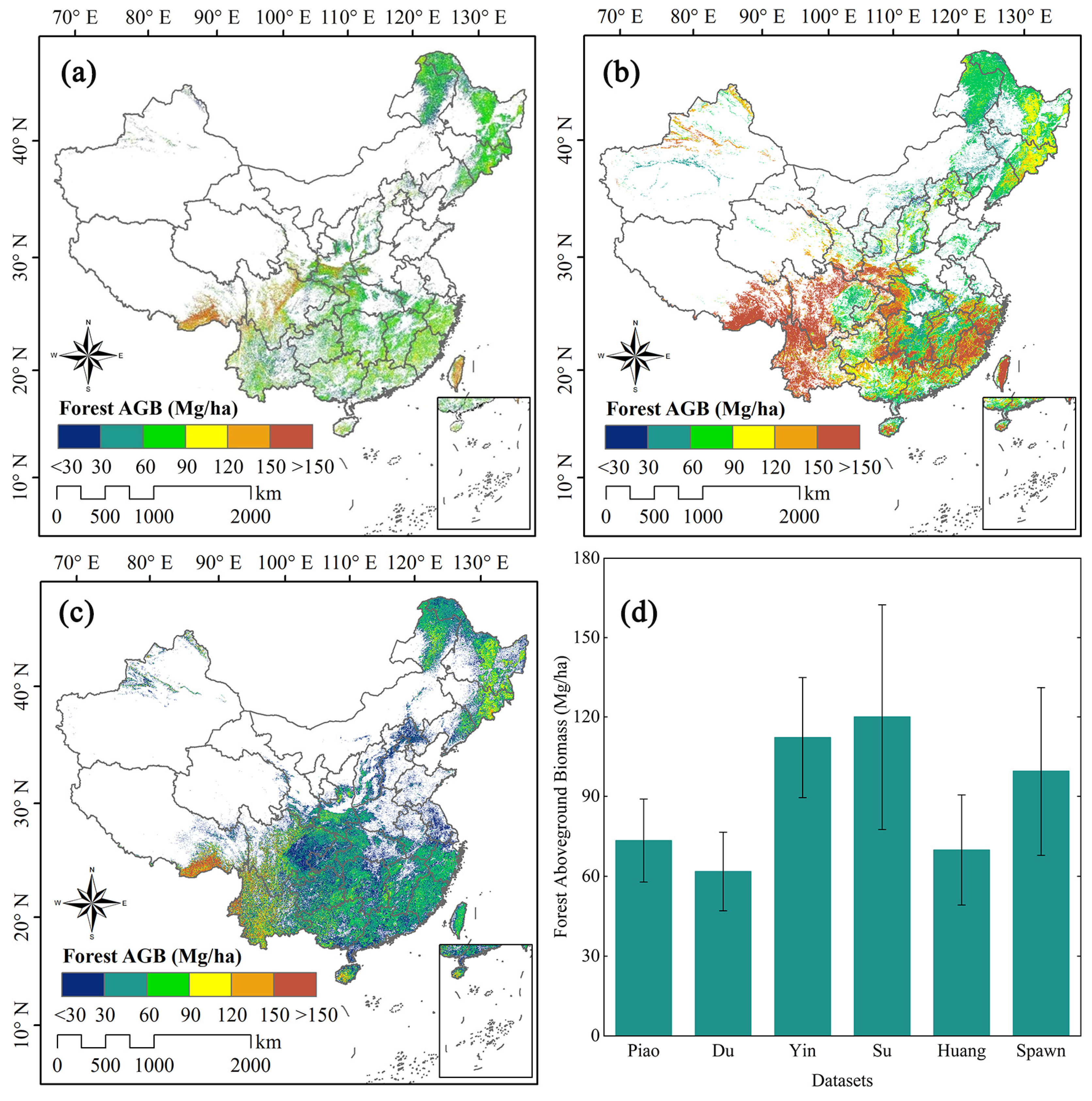
| Sources | Average Forest AGB (Mg/ha) | Resolution (m) | Time Interval |
|---|---|---|---|
| Piao et al. [229] | 73.40 | 8000 | 1981–1999 |
| Du et al. [230] | 61.80 | ~5600 | 2004–2008 |
| Yin et al. [231] | 112.20 | 1000 | 2001–2013 |
| Su et al. [232] | 120.00 | 1000 | 2004 |
| Huang et al. [25] | 69.88 | 30 | 2006 |
| Spawn et al. [233] | 99.50 | 300 | 2010 |
Disclaimer/Publisher’s Note: The statements, opinions and data contained in all publications are solely those of the individual author(s) and contributor(s) and not of MDPI and/or the editor(s). MDPI and/or the editor(s) disclaim responsibility for any injury to people or property resulting from any ideas, methods, instructions or products referred to in the content. |
© 2023 by the authors. Licensee MDPI, Basel, Switzerland. This article is an open access article distributed under the terms and conditions of the Creative Commons Attribution (CC BY) license (https://creativecommons.org/licenses/by/4.0/).
Share and Cite
Tian, L.; Wu, X.; Tao, Y.; Li, M.; Qian, C.; Liao, L.; Fu, W. Review of Remote Sensing-Based Methods for Forest Aboveground Biomass Estimation: Progress, Challenges, and Prospects. Forests 2023, 14, 1086. https://doi.org/10.3390/f14061086
Tian L, Wu X, Tao Y, Li M, Qian C, Liao L, Fu W. Review of Remote Sensing-Based Methods for Forest Aboveground Biomass Estimation: Progress, Challenges, and Prospects. Forests. 2023; 14(6):1086. https://doi.org/10.3390/f14061086
Chicago/Turabian StyleTian, Lei, Xiaocan Wu, Yu Tao, Mingyang Li, Chunhua Qian, Longtao Liao, and Wenxue Fu. 2023. "Review of Remote Sensing-Based Methods for Forest Aboveground Biomass Estimation: Progress, Challenges, and Prospects" Forests 14, no. 6: 1086. https://doi.org/10.3390/f14061086
APA StyleTian, L., Wu, X., Tao, Y., Li, M., Qian, C., Liao, L., & Fu, W. (2023). Review of Remote Sensing-Based Methods for Forest Aboveground Biomass Estimation: Progress, Challenges, and Prospects. Forests, 14(6), 1086. https://doi.org/10.3390/f14061086