Article

Identifying the Relationships between Landscape Pattern and Ecosystem Service Value from a Spatiotemporal Variation Perspective in a Mountain–Hill–Plain Region

1
College of Resources and Environmental Sciences, Henan Agricultural University, Zhengzhou 450046, China
2
Henan Engineering Research Center of Land Consolidation and Ecological Restoration, Henan Agricultural University, Zhengzhou 450046, China
3
Henan Institute of Geophysical Spatial Information Co., Ltd., Zhengzhou 450009, China
*
Authors to whom correspondence should be addressed.
Forests 2023, 14(12), 2446; https://doi.org/10.3390/f14122446
Submission received: 19 October 2023 / Revised: 10 December 2023 / Accepted: 11 December 2023 / Published: 14 December 2023
(This article belongs to the Special Issue Ecosystem Services and the Forest Economy)

Abstract

:
Identifying the changes in landscape pattern and ecosystem service value (ESV) and clarifying their relationship in temporal changes and spatial variations can provide insight into regional landscape features and scientific support for regional landscape planning. Leveraging land use data from the Yihe River Basin, we quantitatively assessed the landscape pattern and ESV shifts spanning from 2000 to 2018 using the landscape pattern indexes and the equivalence factor method. We employed Pearson correlation metrics and the geographically weighted regression model to explore the interrelation of their spatiotemporal variations. Our results show the following: (1) Forestland represents the most expansive land cover category. Apart from construction land, all other types experienced a decline in area. The most notable change occurred in the area of construction land. (2) The aggregation of the overall landscape shows a downward trend. The levels of fragmentation, landscape diversity, and richness increased. (3) Throughout the entire study period, the overall ESV gradually decreased, and the land cover type with the greatest contribution to the ESV was forestland. (4) In terms of temporal changes, the patch density and edge density of the overall area are significantly negatively correlated with total ESVs. The largest values for the patch index, perimeter–area fractal dimension (PAFRAC), and aggregation are significantly positively correlated with total ESVs. (5) In terms of spatial variation, the contagion index (CONTAG), PAFRAC, and the Shannon diversity index (SHDI) were noticeably correlated with ESVs. The CONTAG is positively correlated with ESVs upstream, but negatively midstream and downstream. The SHDI is negatively correlated with ESVs upstream, but positively midstream and downstream. The PAFRAC exhibits a positive correlation with ESVs for the most part. The association between the landscape pattern indexes and ESVs exhibits temporal and spatial inconsistencies in most instances, suggesting a spatiotemporal scale effect in their relationship. This study recommends that the local government devises a long-term strategy for urban development and exercises stringent control over the unregulated expansion of construction land. Through reasonable territorial spatial planning, government departments could enhance the connectivity of the overall landscape pattern of the Yihe River Basin to achieve the reasonable allocation and sustainable development of regional resources.

1. Introduction

Ecosystem services encompass the products and functions of ecosystems that enhance human well-being and contribute to both survival and the overall quality of life [1], including provisioning services, regulating services, cultural services, and supporting services. Ecosystem service value is the ecological service benefits that humans derive from ecosystems [2], as well as the expression of ecosystem functions and utilities [3], which is abbreviated throughout as ESV. Landscape patterns, involving the spatial arrangement and diverse sizes and shapes of landscape elements, serve as a crucial metric in assessing the quality of regional ecological environments [4]. The dynamic changes in landscape patterns record the interactive process between human activities and the natural environment, specifically manifesting as changes in land use conditions [5]. Land use is an important foundation for regional human activities and economic development. With the development of technology and the continuous acceleration of urbanization, people’s land use intensity is increasing, and the impact on the ecological environment is growing. As per the 2005 Millennium Ecosystem Assessment report by the United Nations, more than 60% of ecosystem services have undergone degradation over the last 50 years [2]. Extensive human activities, particularly rapid urbanization [6] and coal mining [7,8], significantly impact the value of ecosystem services by causing substantial changes in landscape patterns and ecosystems. Therefore, examining the influence of alterations in landscape patterns on ESV and comprehending their dynamic shifts can aid in determining both the losses and gains within the ecological environment. This understanding serves as a scientific foundation for fostering basic economic development and implementing sustainable landscape management practices [9,10].
Heterogeneous landscapes affect the flow of matter and energy in ecosystems and therefore control ecosystem processes [11,12]. Changes in landscape structure will interfere with these ecosystem processes, resulting in the degradation of ecosystem functions and changes in ESV [13,14]. Dynamic changes in landscape patterns are closely related to ESV [15,16]. In recent years, research on the connections between ecosystem services and landscape patterns has become increasingly popular for large-scale areas such as cities [17,18,19,20], river basins [21,22,23], wetlands [24,25,26], and coastal zones [27]. Additionally, researchers have focused on small-scale areas, such as central urban areas [28], ecological protection areas [29,30], forests [31,32], farmlands [33,34], citrus orchards [35], and other areas. Existing studies have found that the contributions of different landscape types to ESVs vary [36] and different patterns of landscape changes may have positive or negative impacts on ESV. In the European Alps and New Zealand hill country, Vigl et al. [36] and Tran et al. [37] have respectively explored the correlations between landscape structure and the provision of ecosystem services. The alteration of landscape patterns significantly influences the provision of ecosystem services, given that distinct landscape structures yield varying types and quantities of such services. In the Bay Area and Zhoushan Islands, Cao et al. [38] and Tong et al. [39] investigated alterations in landscape patterns and ESV characteristics. Their findings indicate that the reciprocal transformation among various landscape types enhances the diversity of landscapes per unit area in the studied region, consequently resulting in an overall increase in the total ESV. However, Xu et al. [40] found in their studies in Wenchuan County that not all changes in landscape patterns cause variations in ecosystem services.
Additionally, some studies have found that changes in landscape patterns influence the landscape index, and different landscape indexes have dissimilar losses and benefits to ESVs. For example, Mitchell et al. [41] and Grêt-Regamey et al. [42] demonstrated how landscape fragmentation affects ecosystem services by modifying the configuration and spatial arrangement of landscape patches. Zheng et al. [43] conducted a study on the ESV in the South Jiangxi area from 2000 to 2018, revealing a positive correlation between the ESV and the contagion index, and a negative correlation with the Shannon diversity index. Their findings suggest that when landscape types exhibit a greater diversity, their aggregation increases, contributing positively to the overall enhancement of ESV. Wen and Li [44] analyzed Guizhou’s land use change patterns and its ESV and concluded that rising diversification and diminishing fragmentation positively influence regions characterized by high-value landscape types. However, in areas with low-value landscape types, the opposite effect is observed.
Numerous studies have examined the relationship between landscape patterns and ESVs via correlation analyses, but most of them ignore the spatial heterogeneity of variables. Changes in landscape patterns are spatially heterogeneous, so when analyzing the correlation between landscape pattern indexes and ESV changes, the spatial characteristics of variables should be fully considered to reflect the spatial changes of the impacts. Additionally, different landscape types lead to dissimilar changes in landscape patterns, which have varied effects on ecosystem services. Therefore, no consensus exists on the relationship between different landscape pattern indexes and ESV, especially when the effects of time changes or space changes are considered. In view of this, by considering temporal changes or spatial heterogeneity, the relationships between landscape patterns and ESV could be fully identified to support landscape planning.
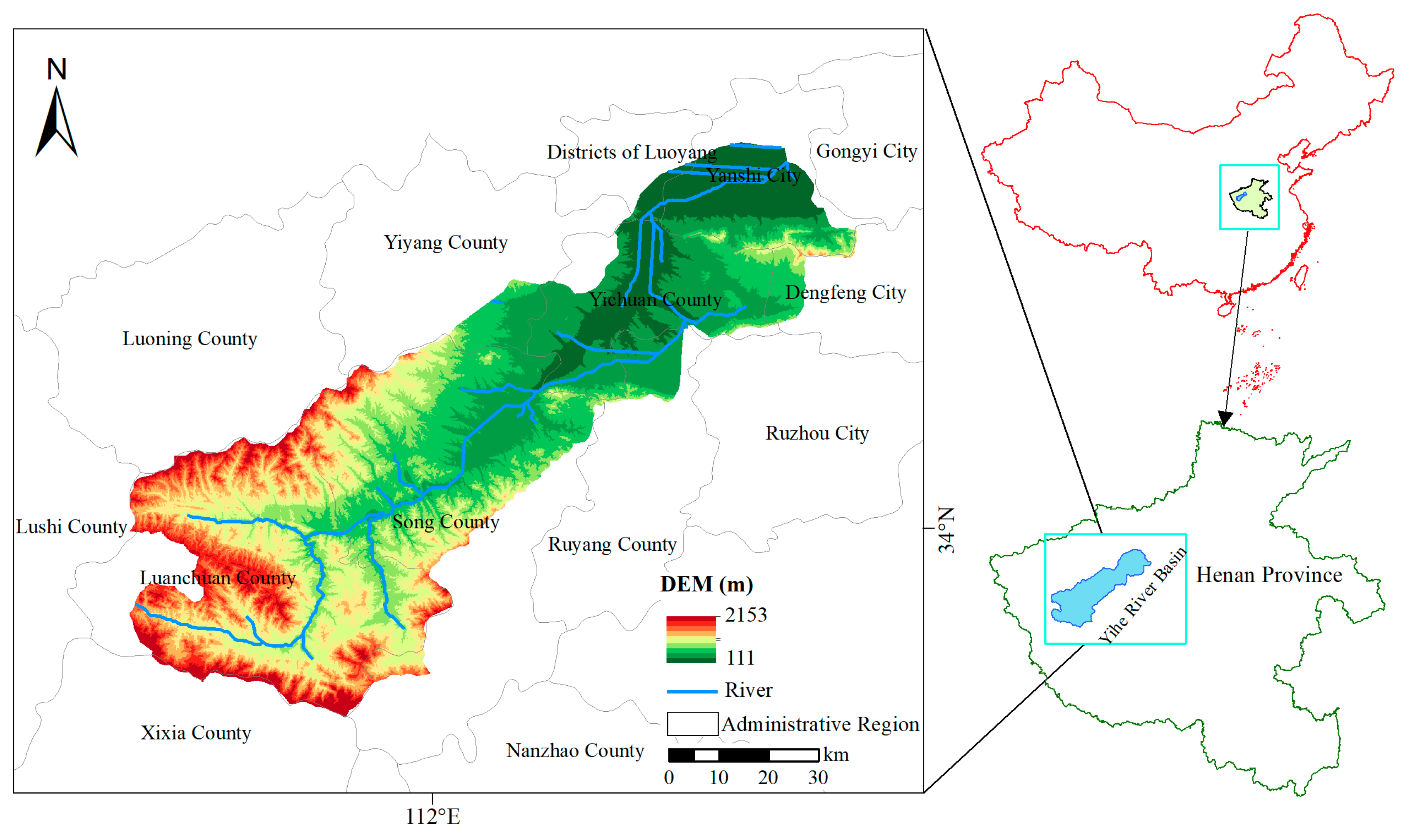
Situated in the western region of Henan Province, the Yihe River Basin has been influenced by human activities for an extended period due to its early development. It boasts diverse ecosystem types and abundant resources, thus holding considerable ecological value. The importance of the Yihe River Basin is reflected in its provision of water resources to local communities, agricultural support, and promotion of economic activities. The river has a profound impact on local sustainable development and human livelihoods. As a result of these characteristics, the Yihe River Basin serves as a pivotal study area, exemplifying the impact of landscape pattern changes on ESVs. Although the existing research methods on the response mechanism of ESV caused by changes in watershed landscape patterns are relatively mature, they are mostly concentrated in the Yangtze River, Yellow River Basin, and their tributaries [22,45,46,47,48,49,50]. On the contrary, little attention has been paid to the empirical analysis of the relationship between landscape patterns and ESVs in the typical mountain–hill–plain areas with abundant natural resources in the Central Plains [51], which need further study. To sum up, this research analyzes the relationship between landscape patterns and ESVs in the Yihe River Basin spanning from 2000 to 2018 from the perspective of spatiotemporal variation. Our research aims to achieve three primary goals: (1) analyze the spatiotemporal variation in landscape patterns and ESV in the Yihe River Basin; (2) examine the relationship of temporal changes in landscape pattern indexes and ESV using Pearson correlation coefficients; and (3) explore the relationship of spatial variations in landscape pattern indexes and ESV through a geographically weighted regression. This research contributes to broadening our knowledge of the current state of ecosystem services in the region, offering a valuable scientific reference for future sustainable resource utilization, landscape planning, and ecological protection endeavors.

2. Materials and Methods

2.1. Study Area

The geographical location of the Yihe River Basin is 111°16′ E–112°47′ E, 33°42′ N–34°47′ N (Figure 1). The Yihe River Basin, situated in the western part of Henan Province, falls within the climatic zone characterized by temperate continental monsoons. July and August experience the highest temperatures, while January sees the lowest. The annual average temperature ranges from 11 to 15 °C with a frost-free period of 216 days, an average wind speed of 1.2 m/s, and 2029 h of total sunshine. In the upper basin, total precipitation, average wind speed, and sunshine hours are higher, but annual average temperature, frost-free days, average ground temperature, and total evaporation are smaller. Rainfall is primarily from natural precipitation, unevenly distributed throughout the year. Approximately 50% of precipitation occurs from July to September, leading to frequent heavy rains and associated disasters, like floods, landslides, collapses, and mudslides. The basin features numerous water storage, hydropower, and irrigation projects. The area of the basin is 6100 km2 [52,53]. The general topography exhibits higher elevations in the southwest and lower elevations in the northeast. Abundant natural landforms characterize the basin, primarily encompassing mid-range mountains, low mountains, hills, river valleys, and plains. The vegetation in our site is diverse, displaying clear vertical distribution influenced by altitude. At 750 to 1600 m, warm temperate deciduous broad-leaved forests dominate, featuring tree species from the northern temperate zone. Between 1600 and 1900 m, coniferous and deciduous broad-leaved mixed forests prevail. The basin encompasses over 10 soil types, with cinnamon soil and brown loam soil dominating the watershed. Brown soil is prevalent in the upper reaches, while cinnamon soil extends across the upper, middle, and lower reaches. Our site has a gross national product of 133.637 billion CNY and a total population of 2.4221 million. Per capita GDP varies, with the lower reaches significantly exceeding the upper and middle reaches. Abundant in mineral resources, Luanchuan County stands out as a renowned polymetallic mineral concentration area in China. The basin’s topography in the middle and lower reaches is flat, concentrating primary industry development in this area. Rich in tourism resources, the basin’s economic development is stimulated. As a whole, it is a mountainous landscape with rich natural and cultural landscapes.
This research focused on the Yihe River Basin for three primary reasons. Firstly, the basin’s location in the transitional zone between north and south and east and west geographical environments results in a diverse range of environmental types, despite the complex river channel shape and the fragile and sensitive ecology. Secondly, our site is a vital populated area for both population activities and economic development within the broader Yellow River Basin. Its strategic importance is crucial for the overall ecological protection and high-quality development of the Yellow River Basin. Lastly, our site exhibits a pronounced disparity between the supply and demand of ecosystem services, particularly in terms of water resources. Urgent clarification of the relationship between landscape patterns and ecosystem services is necessary to provide scientific support for optimizing landscape configuration and implementing rational landscape planning.

2.2. Data Sources

The main data used in this paper are outlined below. Land use data with a spatial resolution of 30 m for five phases (2000, 2005, 2010, 2015, and 2018) within the Yihe River Basin were sourced from the Resources and Environment Science Data Center of the Chinese Academy of Sciences (http://www.resdc.cn accessed on 16 January 2023). The accuracy of the land use data, verified through on-site selection, exceeds 85% [52]. Socioeconomic statistical data are from the China Statistical Yearbook (http://www.stats.gov.cn/sj/ndsj/ accessed on 16 January 2023), the Henan Provincial Statistical Yearbook (https://tjj.henan.gov.cn/tjfw/tjcbw/tjnj/ accessed on 16 January 2023), and the Statistics Station of Henan Provincial Bureau of Agriculture. Considering the land cover types and the current state of land development and utilization in the Yihe River Basin, the land cover data were remerged and categorized into six types using ArcGIS software. Forestland encompasses areas supporting the growth of trees, shrubs, and bamboo, including land with trees, shrub areas, open woodland, and other types of woodland. Grassland includes diverse herbaceous-plant-dominated areas with a coverage exceeding 5%. Cultivated land encompasses areas where crops are grown or flat land that has been under cultivation for over three years. Construction land comprises urban and rural residential zones, as well as industrial, mining, transportation, and other developed areas. Water areas encompass natural bodies of water and land used for water conservancy facilities. Unutilized land refers to presently unused land, including areas that pose usage challenges.

2.3. Quantifying the Spatiotemporal Variation in Landscape Patterns and Ecosystem Service Values

2.3.1. Land Cover Dynamics

Land cover dynamics can fully show the changes in landscape types, and it is an important indicator for analyzing the dynamic changes in landscape patterns. This pertains to the extent of alterations in the quantity of a specific landscape type within the research area over a defined time frame, serving as an indicator of both the magnitude and average speed of change in land cover types [21]. Its mathematical expression is as follows [54]:
K = U i U j U j × 1 T × 100 %
where K is the land cover dynamics; Uj is the area of a certain land cover type in the early stage of study, in hm2; Ui is the area of a certain land cover type in the late stage of study, in hm2; and T is the study time quantum.

2.3.2. Landscape Pattern Index

Referring to relevant studies in the literature [55,56,57,58,59], based on the ecological significance of different landscape pattern indexes, many representative indicators that have already been formed are selected by combining the landscape characteristics of the Yihe River Basin and our actual needs in this study. The common indicators are selected based on the level of patch type and landscape scale: percentage of landscape (PLAND), landscape shape index (LSI), patch density (PD), patch cohesion index (COHESION), mean patch size (MPS), landscape division index (DIVISION), largest patch index (LPI), perimeter–area fractal dimension (PAFRAC), aggregation index (AI), Shannon diversity index (SHDI), contagion index (CONTAG), and edge density (ED) (Table 1). PLAND and LPI indicators serve to elucidate the landscape structure and proportions within the watershed, aiding in the identification of dominant landscape types. LSI and PAFRAC indicators provide insights into the complexity of landscape patch shapes. For the PAFRAC, as the fractal dimension approaches 1, the shape tends towards a square, while a value closer to 2 signifies increased perimeter twists, indirectly indicating the level of landscape aggregation and fragmentation. PD, DIVISION, and ED indicators convey information about landscape fragmentation and heterogeneity, in which higher values indicate increased fragmentation and heterogeneity. COHESION and MPS indicators gauge the degree of aggregation of patch types, aiding in the identification of connectivity status for specific patch types. Larger COHESION and MPS values indicate better connectivity for a particular patch type. SHDI reflects landscape diversity, characterizing the richness and intensity of heterogeneity, and it is sensitive to the distribution status of patches. Larger SHDI values signify a more diverse watershed landscape. AI and CONTAG indicators indicate the degree of aggregation or the extension trend in landscapes at the overall landscape scale, helping to discern the connectivity status of watershed landscapes. Larger AI and CONTAG values suggest improved landscape aggregation and reduced landscape dispersion. These selected indicators comprehensively capture various aspects of the landscape and are closely tied to key ecological processes and functions. Changes in these landscape indicators can influence ecosystem service values (ESVs). Monitoring and quantifying these indicators lay the groundwork for understanding the relationship between landscape patterns and ESV. The quantitative analysis of spatiotemporal changes in landscape patterns within the Yihe River Basin, spanning from 2000 to 2018, is conducted using Fragstats 4.2 and ArcGIS 10.0. The landscape pattern index of overall basin changes in time is directly produced using Fragstats 4.2. The spatial distributions of the landscape pattern index are obtained using the 1 km × 1 km moving window method.

2.3.3. Ecosystem Service Value Evaluation

Quantitative evaluation of ESV involves landscape ecology, ecological economics, environmental science, land resource management science, and other frontier fields [60] and is one of the core issues of international sustainable development. In 1997, Daily first elaborated and analyzed ESV at a theoretical level [61]. In the same year, Costanza and some scholars from the United States assigned corresponding ecological value coefficients to different types of ecosystems on a global scale to indirectly calculate ESV [62]. However, this evaluation method cannot be used to directly calculate China’s ESV. Therefore, based on their studies, Chinese scholars such as Xie et al. [63,64,65] constructed an ESV equivalent table per unit area that would be suitable for China, which is one of the commonly used methods for quantitatively evaluating ESV in China today. The ESV equivalent table serves the purpose of distinguishing various types of ecosystem services and standardizing the quantification of each service to derive the overall ecosystem service value. To assess ESV, one needs data on the area of distribution of the ecosystem to revise the ecosystem service value equivalent factor table. Drawing upon the Evaluation Model of China’s Ecosystem Service Value developed by Xie et al. [63,64,65], we made necessary adjustments by integrating the specific conditions of the Yihe River Basin. Revising the ESV coefficients to be specific to our study area enables a more precise reflection of the region’s actual conditions. This adjustment ensures greater accuracy of the parameters within the ESV equivalent table. Consequently, the refinement contributes to enhancing the reliability of assessment outcomes, as well as refining the regional specificity and practical applicability of the results. Ultimately, this targeted refinement could provide more nuanced support for informed scientific decision making. Modification method based on grain yields was applied to the Equivalent Table of Ecosystem Service Value per Unit Area of Land Ecosystems in China, resulting in the creation of the Henan Ecosystem Service Value Equivalent Table. It is noteworthy that the ESV coefficient of construction land was not determined in the method of Xie et al. [63,64,65], and other studies [66,67] were referenced to define the ESV coefficient of construction land. Utilizing fundamental data, such as the planting area of grain crops, grain yield per unit area, and prices in Henan Province from 2000 to 2018, we calculated the economic value of the primary grain crops per unit area. The economic value provided by natural ecosystems is 1/7 of the existing research area’s main grain crops [22]. The equivalence factor of ESV in the Yihe River Basin is calculated as 1519.98 CNY/hm2. Finally, the ESV per unit area is determined. The formulas are shown below:
E 1 = Q × F 7
E x = a x × E 1
In Equations (2) and (3), E1 represents the economic value of the ESV per unit in Henan Province, while Q denotes the average grain yield of Henan from 2000 to 2018 (5338.08 kg/hm2); F is the average purchase price of grain in Henan Province during the research period (1.9932 CNY/kg); Ex is the ESV coefficient of type x land per unit area; and ax is the ESV equivalent (x = 1, 2, 3, …, 6). The ecosystem service value coefficient per unit area in the Yihe River Basin is obtained (Table 2).
The formulas for ESVs are as follows:
E S V = i = 1 n A i × V C i
In Equation (4), ESV is the ecosystem service value, in CNY; n is the number of land cover types; Ai is the area of type i landscape, in hm2; and VCi is the ESV coefficient of type i land cover, in CNY/hm2.

2.4. Quantifying the Correlations between Landscape Patterns and Ecosystem Service Values

2.4.1. Correlation Analysis in Temporal Change

Pearson correlation coefficient is a common statistical method to examine the correlation between two things, and it is mainly used to explore the strength of the linear correlation between two independent continuous numerical variables. Pearson correlation coefficient is calculated using Statistic Package for Social Science (SPSS) 26.0. Pearson correlation coefficient is used as an indicator to conduct a significance analysis and examination of the correlation in time sequence between landscape pattern indexes and ESVs based on double-tailed t-test. Finally, the correlation coefficients are converted into a heat map in Origin 2021.

2.4.2. Geographically Weighted Regression in Spatial Variation

In our study, we employ a geographically weighted regression model to assess the associations between landscape patterns and ecosystem service values. The geographically weighted regression model, using a spatial analysis method, is utilized for parameter estimation, building upon the principles of the conventional regression model. Geographically weighted regression applies the spatial weight matrix to the linear regression model. The model coefficients can better explain the spatial heterogeneity of geographic elements and solve the problem of spatial non-stationarity. Using geographically weighted regression to detect the relationships between landscape patterns and ESV, spatial variations mainly occurred at the landscape scale. Therefore, the eight landscape pattern indexes in the landscape scale were selected as the initial variables of model, including PD, DIVISION, LPI, PAFRAC, AI, SHDI, CONTAG, and ED. Due to the redundancy among the landscape pattern indexes, we firstly tested the collinearity of the 8 selected landscape pattern indexes through SPSS26.0 to obtain the variance inflation factor (VIF) (Table 3). VIF is the reciprocal of tolerance (TOLERANCE = 1 − R2), which can reveal collinearity problems between variables. Then we deleted the landscape pattern index, which has larger VIF, and then repeated the collinearity test many times. Finally, the three indexes of PAFRAC, CONTAG, and SHDI were selected as independent variables. We used a geographically weighted regression model to examine the relationship between ecosystem service values and three landscape pattern indexes that passed the collinearity test.
We utilize ArcGIS to conduct analyses using both the ordinary least squares (OLS) model and the geographically weighted regression model. In our calculations [68], the corrected Akaike information criteria (AICc) values for the OLS model are 26,973.205, 26,956.189, and 26,949.857, while for the geographically weighted regression model, they are 26,659.968, 26,668.494, and 26,660.957 Table 4. If the discrepancy in AICc values exceeds 3, the simulation outcomes derived from the geographically weighted regression model are deemed more rational. In the present investigation, the observed difference is much greater than 3, accompanied by a significant elevation in the R2 value of the geographically weighted regression model to 0.541, 0.536, and 0.546. These findings imply that the fitting results obtained from the geographically weighted regression model are more apt for this research.
The calculation formula for the geographically weighted regression model is expressed as follows:
y i = β 0 ( u i + v i ) + k β k ( u i + v i ) x i k + ε i
In the specified equation, yi denotes the dependent variable, while (ui,vi) represent the geographical coordinates of the i-th sample unit. The term xik signifies the value of the k-th independent variable in the i-th sample unit, where k is the number of independent variables, and i is the number of sample units. The symbol εi accounts for the random disturbance term, and βk(ui,vi) indicates the value of the continuous function βk(u,v) in the i-th unit.

3. Results

3.1. Land Cover Changes

The general trend in landscape type changes within the Yihe River Basin spanning from 2000 to 2018 (Figure 2) reveals a predominant increase in the overall extent of construction land. In contrast, the areas of other land cover types exhibit varying degrees of decline during this period (it is noteworthy that the analysis in this paper excludes unused land in the study area, given its negligible landscape coverage). The landscape area of construction land increased by 6654 hm2 from 2000 to 2018. The interval witnessing the most substantial surge in construction land area spanned from 2005 to 2010, registering a noteworthy increase of 3161.4 hm2. This growth is attributed to the robust expansion of the service industry, particularly driven by tourism, concurrent with accelerated socioeconomic development and urban construction. The continuous expansion of the central urban area further amplified the demand for urban land use during this specific timeframe. In addition, with the appeal of the development of tourism throughout the Yihe River Basin, the number of scenic spots in the region rapidly increased, leading to a significant increase in land use for scenic facilities. Ultimately, the area of construction land rapidly increased. The time period from 2005 to 2010 also had the greatest reduction in water area (1867 hm2). In addition to its transformation into construction land, the water landscape has been affected by climate conditions such as precipitation and evaporation. In the past decade, the water volume has decreased, the river runoff has decreased, the river channels have narrowed, and some of the rivers have dried up, resulting in an overall decrease in water landscape area. The period from 2005 to 2010 is also the only time period when the cultivated land area increased. The area increased by 193.67 hm2 because it was affected by the national policy “Measures for Reclamation, Development, and Supplementation of Cultivated Land” during this period. A red line of 1.8 billion acres of cultivated land was set up. The total cultivated land area in China aimed to be at least 1.8 billion acres and above. A significant decrease in cultivated land due to urbanization and industrialization would not be allowed. Throughout the entire study, spanning from 2000 to 2018, there was a marginal reduction in both cultivated land and forest land. This minimal change can be attributed to the proactive measures implemented by the local government to staunchly safeguard cultivated land and forested areas.
Table 5 shows the dynamics of various land cover types in the Yihe River Basin during the study period from 2000 to 2018. The rates of changes in each land cover type in the Yihe River Basin from 2000 to 2018 in descending order are as follows: construction land (2.05%) > water area (−0.99%) > grass land (−0.15%) > cultivated land (−0.10%) > forest land (−0.02%). With the exception of construction land, which consistently exhibits a positive dynamic degree, the dynamic degrees of the other land cover types are positive only in one to two time periods and negative in the majority of the periods. The area of construction land was consistently increasing throughout the entire research period, whereas the other land cover types were mainly moving toward negative growth and reductions. Over the four study periods, construction land exhibits the most active t dynamism, with dynamic degrees of 1.00%, 3.35%, 1.81%, and 0.83%. These values significantly surpass those of the other landscape types within the corresponding periods. The forest landscape is opposite to the construction land landscape. This type of landscape has the minimum dynamic degrees, namely, −0.00%, −0.06%, −0.02%, and −0.01%, and is the most stable landscape type. Between 2005 and 2010, excluding the cultivated land landscape, the dynamic degrees of the other landscape types surpass those observed in other study periods. The changes in landscape types are the highest during this period, which correspond to the great increase in construction land. Moreover, the industrial system due to tourism developed rapidly, society underwent rapid changes, and the landscape type structure was significantly adjusted accordingly. The main change is that the other landscape types were transformed into construction land. Overall, except for the construction land landscape, the dynamic degrees of the other landscape types are relatively small, with insignificant changes.
From 2000 to 2018, the transfer area between the six land use types in the Yihe River Basin was 26,448.03 hectares, accounting for about 4.46% of the total area. Figure 3 shows that in 2000, there was little transfer between land uses, but after 2005, there was an increase in transfers between land use types. In general, the conversion of forest land, grassland, and water area to cultivated land was obvious from 2005 to 2010 and from 2015 to 2018. In addition, the areas of cultivated land and construction land were transferred to each other the largest during the study period. Overall, water areas registered the highest transfer-out proportion, while construction land exhibited the highest transfer-in proportion.

3.2. Spatiotemporal Variations in Landscape Patterns

3.2.1. Landscape Pattern Changes at the Level of Patch Type

Figure 4 illustrates alterations in landscape pattern indexes for the different land cover types at the patch level in the Yihe River Basin (unused land is not analyzed due to its small proportion).
Cultivated land and forest land account for a large, stable proportion at around 40% and 45% (Figure 4a), respectively, which are absolutely dominant throughout the whole study period. The land cover type proportion indexes do not change much throughout the whole research period and remain stable, indicating minimal changes in the landscape structure. Only the LSI of the water shows a decrease, whereas the landscape shape indexes of the other land cover types exhibit an upward trend (Figure 4b). The LSI of cultivated land is the largest, showing a stable upward trend, which reflects the fact that the shapes of cultivated land patches tend to be irregular. In comparison to the other land cover types, the construction and cultivated land landscapes consistently exhibit high PD values (refer to Figure 4c), indicating notable fragmentation, a characteristic associated with the region’s terrain. Large proportions of mountainous and hilly areas are in the Yihe River Basin. This area belongs to the mountainous landscape, with scarce land resources. In a period of social progress, the land on slopes or in valleys is occupied by construction and cultivated land, which increases the PD of the construction and cultivated land landscapes. Moreover, the PD of construction land demonstrates an upward trend from 2005 to 2015. This trend is attributed to the predominant increase in construction land occurring in smaller areas, whereas substantial expansions in larger areas are relatively infrequent. Within the Yihe River Basin, cultivated land and forest land serve as the matrix for the landscape, boasting cohesion indexes of 99.8% and 99.9%, respectively (Figure 4d). The landscapes of cultivated land and forest land are highly clustered, concentrated in distribution, and have a good level of connectivity. The cohesion degree of water has shown a downward trend since 2005. The connectivity of water is lowered, which is related to the decrease in the flow of the river system in the Yihe River Basin. The cohesion degree of construction land shows a slow upward trend because the rapid development of the social economy led to a significant increase in the area of construction land, which improves the spatial aggregation of the construction land. The line chart in Figure 4e delineates the average patch area, revealing that forests have the largest average patch area, significantly surpassing that of the other land cover types. Forests exhibit the least fragmentation, boasting superior connectivity and accessibility.

3.2.2. Spatiotemporal Variations in Landscape Patterns at the Landscape Scale

Table 6 shows the time changes in landscape pattern indexes at the landscape scale in the Yihe River Basin. DIVISION and PD reflect the overall degree of landscape fragmentation. Over the whole research period, the DIVISION value first increases, then decreases, and finally reaches its highest value, whereas the PD value shows a gradual upward trend. These changes indicated that the whole landscape in the Yihe River Basin fragments, the patches per unit area increase, and the DIVISION value increases. The LPI shows a downward trend, indicating the dominance of patches in the forest land of the whole landscape decreases. Throughout the entire research period, the PAFRAC consistently demonstrates a downward trend, signaling that each landscape patch type exhibits simplicity and regularity. Overall, the landscape patch types are simpler compared to the initial stage. The aggregation shows a gradual downward trend, which reflects the dispersal of patches in the region and a decrease in the degree of aggregation. The SHDI shows an upward trend, indicating the diversification of patch types in this area and the increasing landscape richness. The reason for this includes the fragmentation of the landscape and the diversity of land types in the Yihe River Basin. The CONTAG is negatively correlated with the ED. The CONTAG shows a downward trend, indicating a reduction in the adjacency probability among different patch types. Landscape factors continue to expand and are dispersed, leading to an enhanced degree of landscape fragmentation. The decline in the CONTAG is due to the fact that during economic development and urban construction, urban construction land continues to encroach on and spread into the surrounding spaces, causing the spread of urban construction lands, which inhibits the spread of other landscapes to a certain extent. During the whole research period, the ED gradually increases, indicating an increase in landscape richness in the region and an increase in landscape heterogeneity. The increase in landscape heterogeneity and richness showed by the ED is mainly due to the increase in land use diversity, the cultivated land and sparse forest land that were formed by reclamation and greening being scattered and embedded in other landscapes, and the enrichment of road networks which destroy the original patch shape.
Figure 5 illustrates the spatial variations in eight landscape pattern indexes at the landscape scale in the Yihe River Basin. Notably, the CONTAG, PAFRAC, and SHDI successfully passed the collinearity test in spatial variation, establishing them as pivotal indexes. The spatial distributions of the remaining landscape pattern indexes closely resemble those of these three key indexes. The CONTAG can reflect the degree of aggregation and dispersion of landscape patches. Spatially, the upper reaches of the Yihe River Basin exhibit a predominantly fragmented distribution in the landscape’s CONTAG, while the contagion situation in the southern part of the middle reaches and the northern part of the lower reaches appears relatively favorable. This indicates a complex degree of clustering among the landscape patches in the Yihe River Basin, but the distribution has clear characteristics. High-value areas are primarily concentrated in the river waterway and regions with flat terrain and fewer buildings, whereas low-value areas are predominantly situated in higher-altitude regions upstream. The CONTAG distribution remains relatively stable throughout the research period, indicating minimal fluctuations in the degree of aggregation and dispersion in the upstream landscape. However, the high-value area in the middle reaches shows an upward trend, and the high-value area in the lower reaches exhibits a trend of shrinking eastward, possibly due to increased construction activities near urban areas and ecological protection in the waterside areas. The PAFRAC could reflect the complexity of characteristics across diverse spatial scales. Spatially, the overall PAFRAC increases from upstream to midstream and increases from west to east downstream. The southern part of the upstream landscape is more complex, and the situation regarding landscape aggregation and fragmentation is diverse and changeable. In the Yihe River Basin, both the northern end of the upstream and the southern part of the midstream show more pronounced changes in landscape characteristics, moving toward a more complex structure. However, overall, the PAFRAC value tends to approach 1, maintaining a relatively regular shape and not showing a high level of fragmentation. The SHDI can reflect the strength of landscape heterogeneity. Spatially, regions characterized by high values of the SHDI are situated in flat zones with low hills and along the western riverbanks downstream. In contrast, low-value areas are predominantly located in elevated mountainous regions upstream. This suggests that the middle and lower reaches are filled with buildings, leading to a fragmented patch distribution and a higher level of landscape heterogeneity, while the upstream landscape is less heterogeneous, with a more uniform patch distribution. The SHDI generally remains unchanged, with only a noticeable increase near Luoyang City’s jurisdiction, indicating an enhanced level of landscape heterogeneity. The rise in landscape heterogeneity and diversity showed by the SHDI primarily stems from ongoing urban expansion and afforestation efforts that continually diminish the share of cultivated land in the overall landscape. The transformation of cultivated land from low crops to construction areas or tall trees and shrubs has altered the once relatively uniform landscape type.

3.3. Spatiotemporal Variations in Ecosystem Service Values

Table 7 shows that the ESVs in the Yihe River Basin in 2000, 2005, 2010, 2015, and 2018 are 124.23 × 10⁸, 124.04 × 10⁸, 121.78 × 10⁸, 121.16 × 10⁸, and 121.04 × 10⁸ CNY. During the whole research period, the ESVs show a steady downward trend, but the decrease is relatively small. Forest land emerges as the predominant contributor to the overall ecosystem service value (ESV). Although the ESV per unit area significantly differs between forest land and water area landscapes (refer to Table 2), the fundamental landscape type in the Yihe River Basin is consistently forest land, maintaining a proportional area of approximately 45%. Therefore, the forest landscape is the main landscape type that controls the total ESV in the Yihe River Basin. Throughout the research period, the ESVs of various landscape types in the late stage remained lower compared to the initial stage. This can be attributed to the partial conversion of four landscape types, namely cultivated land, forest land, grassland, and water area, into construction land. During the period from 2005 to 2010, the total ESV in the Yihe River Basin is decreased the most, and this decrease is much higher than the decrease in other periods, mainly because the changes in various landscape types are large during this period. In particular, the water area landscape is greatly decreased in area, resulting in a much greater decrease in ESV than that of the other landscapes. The decline in total ESV during various research periods and throughout the entire study is intricately linked to the continuous expansion of construction land. In the social development of the Yihe River Basin, the service industry, particularly driven by tourism, has experienced rapid growth. The persistent expansion of industry and the constant surge in demand for construction land have led to the partial conversion of four landscape types, originally characterized by having a high ESV per unit area, into construction land with a lower value per unit area. This factor significantly contributes to the overall decrease in ESV in the Yihe River Basin.
During the study period, the spatial distribution of the ESV in the Yihe River Basin generally showed higher values in the southwest and lower values in the northeast, demonstrating pronounced spatial heterogeneity (Figure 6). The high-value areas of ESV are mainly distributed in the mountainous and hilly areas of Luanchuan County and Song County upstream, where vegetation is abundant and the ecological environment is favorable. Medium-value areas are not only concentrated around high-value regions but also extend to certain sections of the middle and lower reaches. Some of these medium-value regions are situated along the river. Specifically, in the lower reaches, the medium-value areas are predominantly located in the Songshan Mountain region, characterized by dense vegetation, exhibiting a noticeable trend of contraction. Low-value areas are observed in the plains of the middle and lower reaches, featuring a flat topography, sparse forest coverage, and fragmented infrastructure. Negative values are distributed in the areas of Luoyang City’s jurisdiction and Yichuan County. The overall spatial pattern decreases from southwest to northeast, but the distribution of the higher ESVs gradually diminishes, the low-value areas constantly expand, and negative-value areas also gradually increase.

3.4. The Correlations between Landscape Patterns and Ecosystem Service Values

3.4.1. The Correlations in Temporal Change

Landscape pattern changes can be reflected in changes in landscape indexes. The correlations between landscape patterns and ESV in temporal changes can be analyzed through the landscape index of overall area. During the whole research period, the proportion of various land cover types does not change significantly; that is, the landscape structure in the Yihe River Basin does not change much. Therefore, the change in total ESV is relatively small. Figure 7 shows that the PD and ED are significantly negatively correlated with the total ESV, provisioning service value, regulating service value, supporting service value, and cultural service value. The LPI, PAFRAC, and aggregation are significantly positively correlated with the total ESV, provisioning service value, regulating service value, supporting service value, and cultural service value. Additionally, the CONTAG exhibits a significant positive correlation with the provisioning service value, while the SHDI shows a significant negative correlation with the provisioning service value. The DIVISION and Shannon diversity index show an upward trend, indicating an increase in the DIVISION value, landscape heterogeneity, and fragmentation in this area. The LPI and CONTAG aim to measure the dominance of the forest landscape. The two indexes show a downward trend in this area. The supremacy of the dominant landscape, the forest landscape, is slightly decreased, and its aggregation or extension trend is lowered. Overall, the fragmentation of the landscape negatively correlated with the ESV, whereas the centralized distribution, aggregation, and development of natural land cover can improve the ESV. The specific results of this area are that construction land continues to occupy forest land and other natural land types, causing a reduction in the ESV.

3.4.2. The Correlations in Spatial Variations

Based on the geographically weighted regression model, using ESV as the dependent variable and the CONTAG, PAFRAC, and SHDI as explanatory variables, the correlations between landscape patterns and ESV in spatial variations were explored, as shown in Figure 8. Spatially, the CONTAG has negative correlations with the ESV in areas mainly distributed in the middle reaches of Yiyang County, Northwest Song County, and the downstream region, where the CONTAG is higher, and the ESV is distributed in medium- and low-value areas. Positive correlation areas are mainly found upstream, although here the CONTAG is more complex, and the general areas of low CONTAG values show average ESVs, further validating the spatial variation in the correlation between the CONTAG and ESV. It generally presents an “upstream positive correlation, and midstream and downstream negative correlation” distribution pattern, with an overall stable distribution but a noticeable weakening of this correlation downstream. Spatially, the correlation between the PAFRAC and ESV is more scattered, but overall, it is positive. Negative effects are limited to a small southern portion upstream and within the jurisdiction of Luoyang City downstream. Conversely, positive influences are primarily concentrated in the southern part of the upper reaches and the majority of the middle and southeastern lower reaches, with the most profound positive impact occurring at the confluence of the middle and lower reaches. The negative impact in the south end upstream spreads northward over time, while the negative impact in Luoyang City’s jurisdiction slowly shrinks. Spatially, the variation in SHDI regression coefficients shows an overall trend from a negative to positive correlation from the southwest to the northeast. Positive areas are mainly distributed in most of the downstream and middle reaches. In the water landscapes and hilly regions where the SHDI is high, the ESV is also relatively higher compared to that of the surrounding areas. Negative areas are predominantly found in Luanchuan County upstream, particularly in regions with low hills where the SHDI is high but the ESV is lower compared to that of the surroundings. The spatial distribution of the correlations between the SHDI and ESV remains relatively stable, but numerically, the positive degree downstream noticeably diminishes.

4. Discussion

4.1. The Factors of Ecosystem Service Value and Landscape Pattern Changes

The existing literature [69,70,71,72,73] indicates that an expansion in construction land results in a decline in ecosystem service value (ESV). Additionally, reductions in water area, cultivated land, and forest land also contribute to a decrease in ESV. Variations in economic development and land use patterns across different study regions exert diverse impacts on ESV. Wang et al. [74] found that the ESV showed an upward trend with the economic development of Niulanshan–Mapo Town, Beijing. Cheng et al. [75] found the differences in ESV dynamic evolution caused by urban land use changes in China’s megacities from 1995 to 2008. The expansion of construction land, driven by urbanization in the Yihe River Basin, is associated with a decrease in ESV, which aligns with the findings of Zheng et al. [
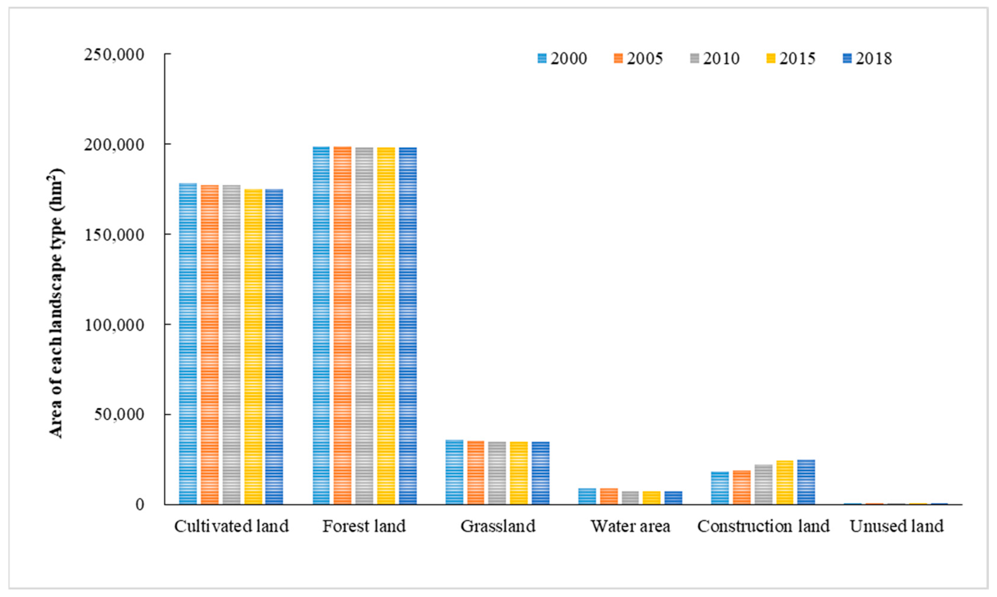
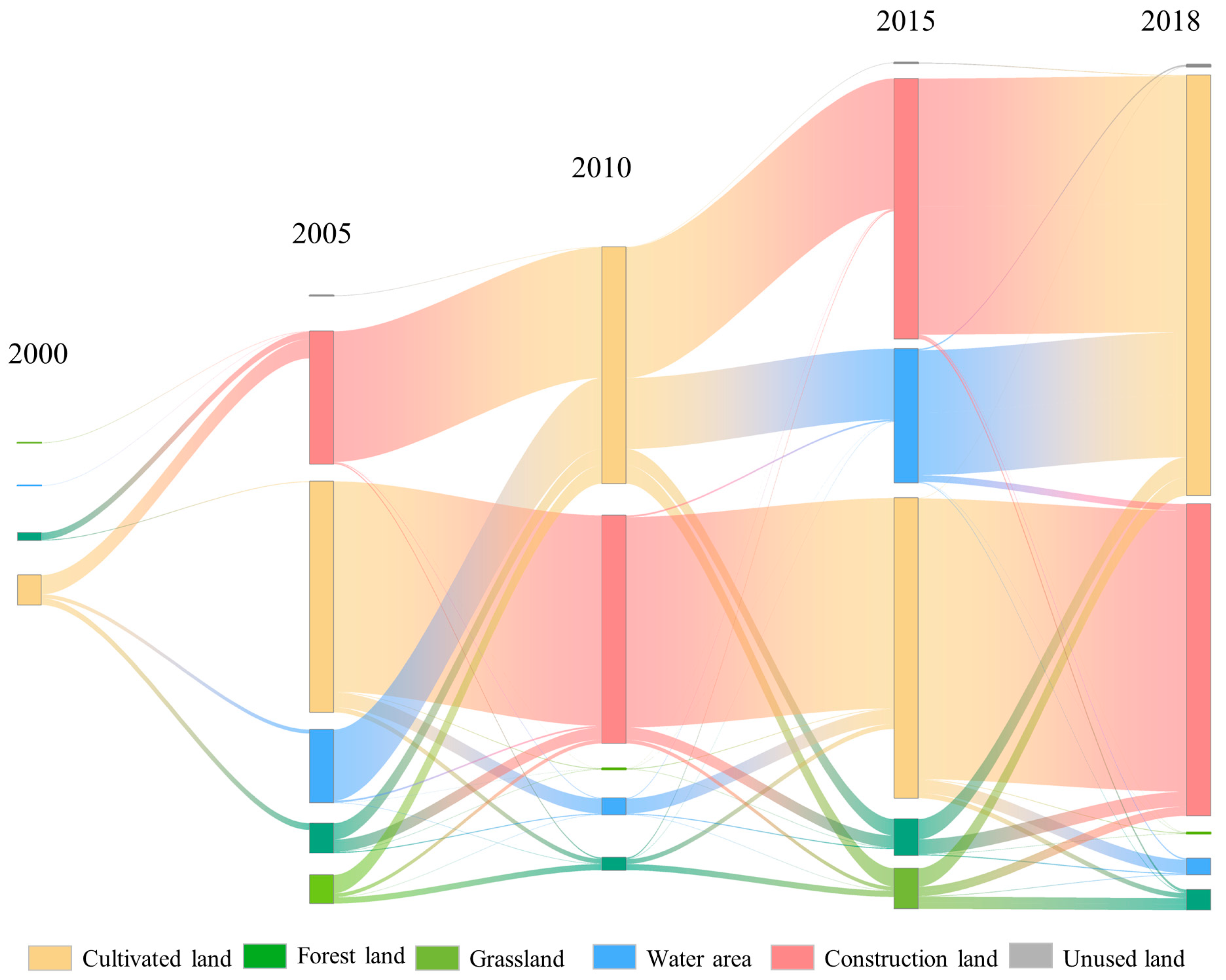
43] and Zou and Zhou [
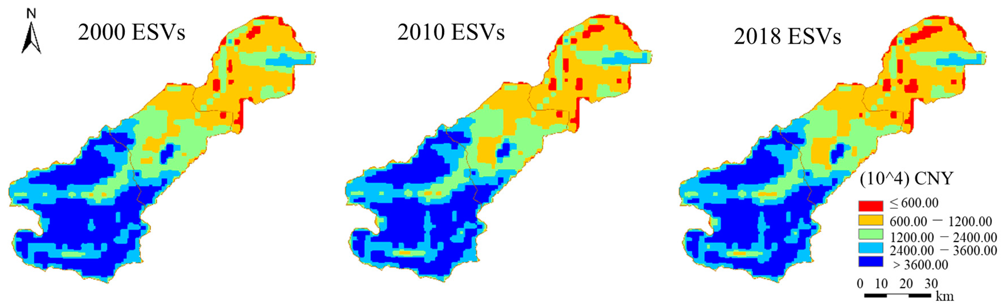
76]. Throughout the study period, while the area of construction land increased in the Yihe River Basin, the other land cover types exhibited a decreasing trend, with minimal changes in cultivated land and forest land. Cultivated land also contributes to food supply, raw material supply, and forest coverage for climate regulation, and the reduction in this transformation promotes a decrease in regional ESV. However, since 2000, the tourism in the Yihe River Basin has gradually become a pillar industry. Notably, the local government’s promotion of “global tourism” led to the establishment of at least one to two tourist areas and numerous tourist villages in each township, intensifying the impact of human-induced construction factors on the natural landscape. Consequently, the area of forest land decreased, contributing to a lower dominance. Moreover, the construction land in different areas of the whole county continues to increase in spots and lines on a small scale, which continuously destroys the integrity of various existing landscapes. Overall, the surge in the growth of construction land can be attributed to swift socio-economic development. The heightened demand for urban land has hastened urban construction and the continual expansion of central urban areas. In 2005–2010, the area of water decreased due to natural and human factors. Among all land cover types, water areas experienced the greatest decrease in area and proportion. The ESV coefficient of water areas is higher than that of the other land cover types, so the transfer of water areas would reduce the overall ESV. In particular, the transformation to construction land severely lowers the ESV. Overall, the total ESV in the Yihe River Basin experienced a decrease of 319 million CNY from 2000 to 2018. The reduction in water area and the increase in construction land emerged as the primary reasons for the ESV decline. Furthermore, forest land and cultivated land were identified as crucial land cover types for sustaining ESV growth. The increase in construction land comes from the transformation of forest land and cultivated land, and a negative ESV coefficient exacerbates the decrease in ESV. The decrease in water area and percentage of forest cover weakens the ecological function of the watershed and consequently erodes the value of services such as gas regulation, hydrological regulation, and climate regulation. Therefore, the proportion of ecological land use in construction land should be increased while protecting the areas of forest land and water and controlling construction land.
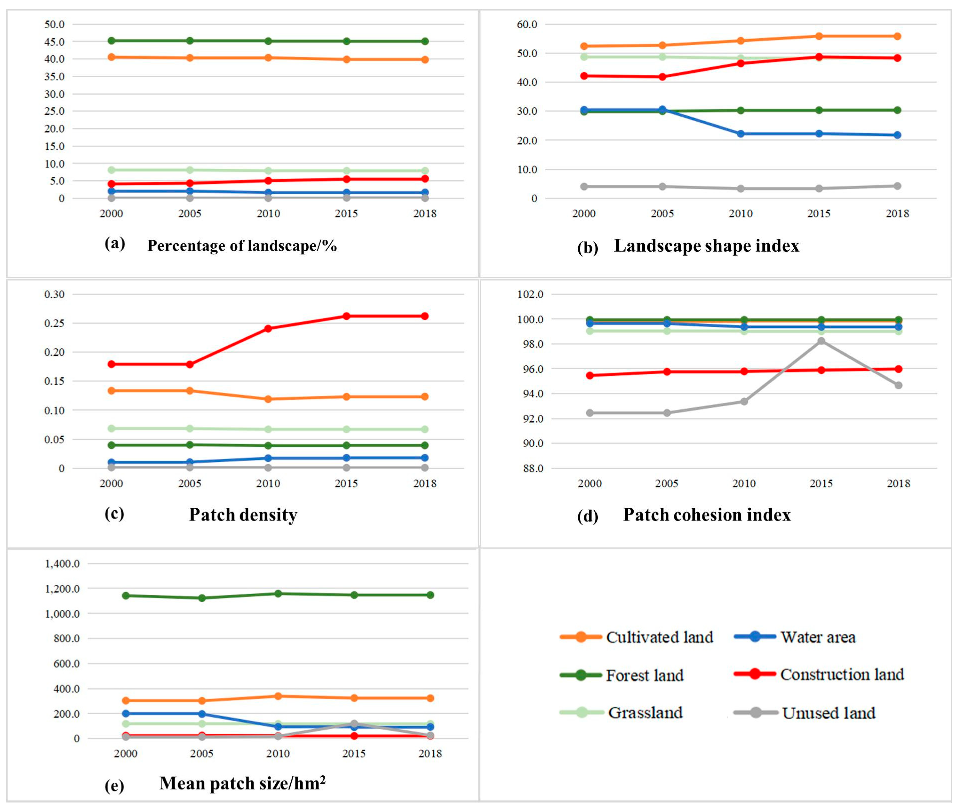
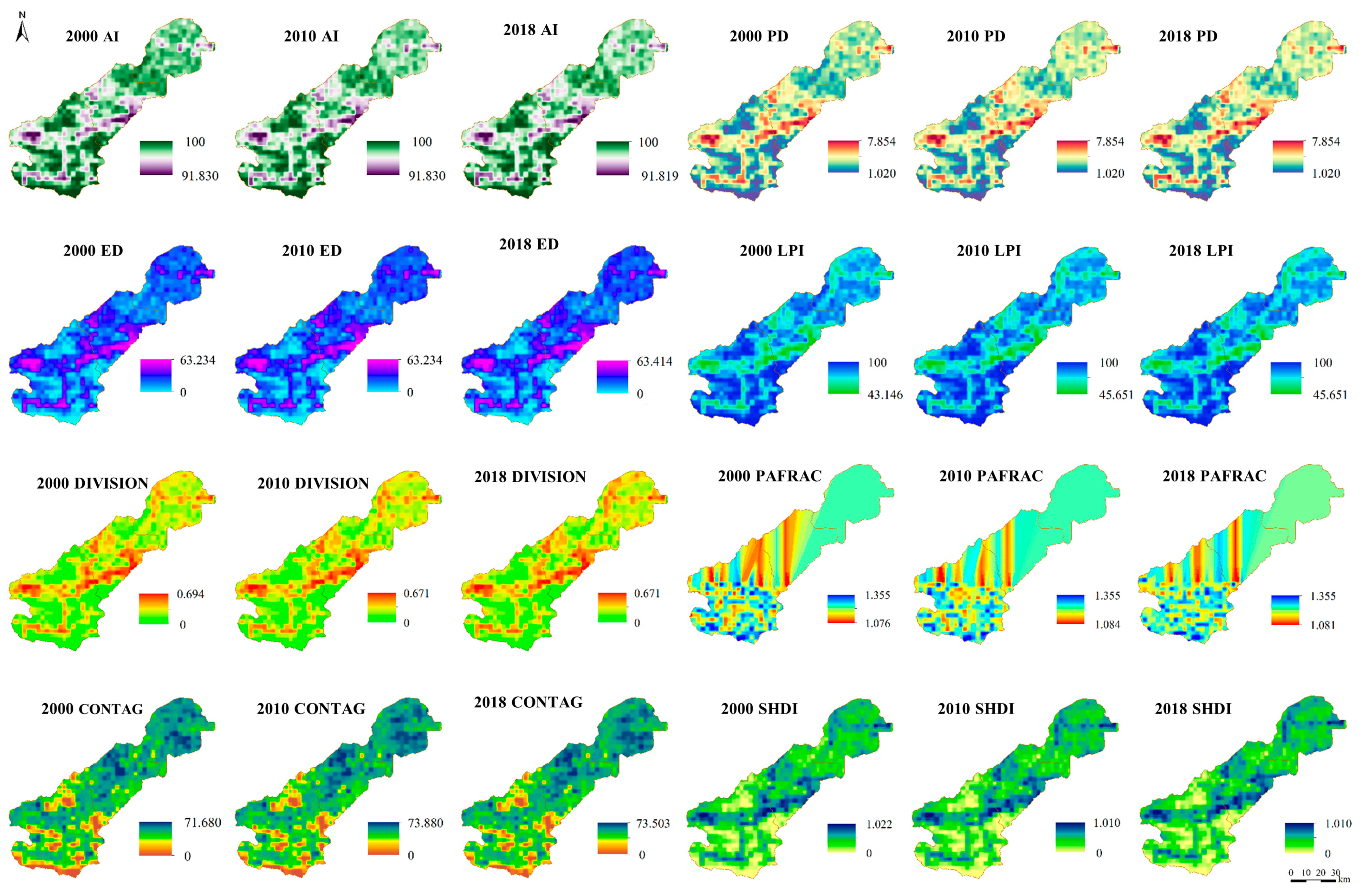
The transformation of the Yihe River Basin’s landscape, as indicated by landscape pattern indexes, results from shifts in spatial structure prompted by various activities, including production and construction. Notably, there was an increase in the coverage of construction land within the overall land composition. Government actions play a pivotal role in shaping both land cover types and the associated ESV. Governmental actions, whether explicit or implicit, notably influence the modifications evident in the landscape configuration. Urban expansion, tourism development, large-scale infrastructure construction, and road network improvements led by the government can cause significant transformations of cultivated land and forestland into construction land and roads, which results in a decline in the LPI and CONTAG values and a rise in the PD and ED values. Road greening, tree planting and afforestation, forest cities, and other governmental measures have increased the proportion of green land, changed the relatively simple landscape structure, and improved the heterogeneity and diversity of the landscape. Under these measures, the SHDI of the landscape increases in the basin. Government measures are a leading factor of landscape pattern changes, which directly or indirectly affect the ESV through policies in the process of social and economic development.

4.2. The Relationships between Landscape Patterns and Ecosystem Service Values

Changes in landscape patterns exert a significant influence on the composition, structure, function, and biochemical processes of regional ecosystems, ultimately leading to fluctuations in ecosystem service value (ESV) [18,76]. Utilizing landscape indexes enables us to conduct a quantitative description of the dynamic alterations in landscape patterns within the study area, providing an effective measure of changes in human activity intensity. Ecosystem services are intricately linked to the structure and ecological processes of the ecosystem within specific temporal and spatial scales, and ESV alterations quantitatively reflect dynamic shifts in landscape patterns.
The influence of landscape patterns on ESVs demonstrates specific regional traits [77]. The relationship between ESVs and landscape pattern indexes fluctuates over various periods, geographical areas, and types of landscapes. In Yanbian Prefecture, Yu et al. [77] observed a significant positive correlation between the ESV and the AI and CONTAG values, while noting a negative correlation with the PD, LSI, and SHDI values. Zhang et al. [78] found that the ESV is negatively correlated with division and the SHDI in the typical karst areas of Northwest Guangxi. Liu et al. [79] found that the increase in aggregation and decrease in the DIVISION value increase the ESV in the Qinling Mountains. In the Guangdong–Hong Kong–Macao Greater Bay Area, Cao et al. [38] found that lower division degrees are more advantageous for enhancing the overall ESV. Conversely, in the southern bank of Hangzhou Bay, Cen et al. [80] discovered that richer land use, leading to a more fragmented landscape and a higher level of diversity, is beneficial for improving the overall service value. Hu et al. [29] found that the ESV was positively correlated with the PD in the area around Tai Lake. Some differences are observed in the impact of landscape pattern indexes on ESVs for different periods, regions, and landscape types. Landscape pattern indexes can characterize the landscape configuration quantitatively and intuitively, but regional differences lead to variances in matrices and the dominant landscape. Equivalent landscape indexes may reflect different spatial pattern characteristics, and their effects on ESVs are different.
Cultivated land and forest land remain pivotal matrix types among the landscape types in the Yihe River Basin between 2000 and 2018. However, due to strong urbanization development and economic activities, the partial transformation of other land types into the construction land aggravates the fragmentation of the landscape and increases the scatter degree. Therefore, the shape becomes more complex. The construction land does not show a patched, concentrated increase, but a sporadic, scattered increase, which continues to encroach on the other land cover types. The expansion of industrial and mining land, tourism land, and urban construction land in the Yihe River Basin has divided the landscape pattern of the ecosystem, resulting in the fragmentation of the natural landscape. It lowers the connectivity of the landscape, destroys the biological habitat, and weakens the support and aesthetic value to result in a lower total ESV. Similar to the findings of Hou et al. [81], Zhang et al. [82], and Wang et al. [
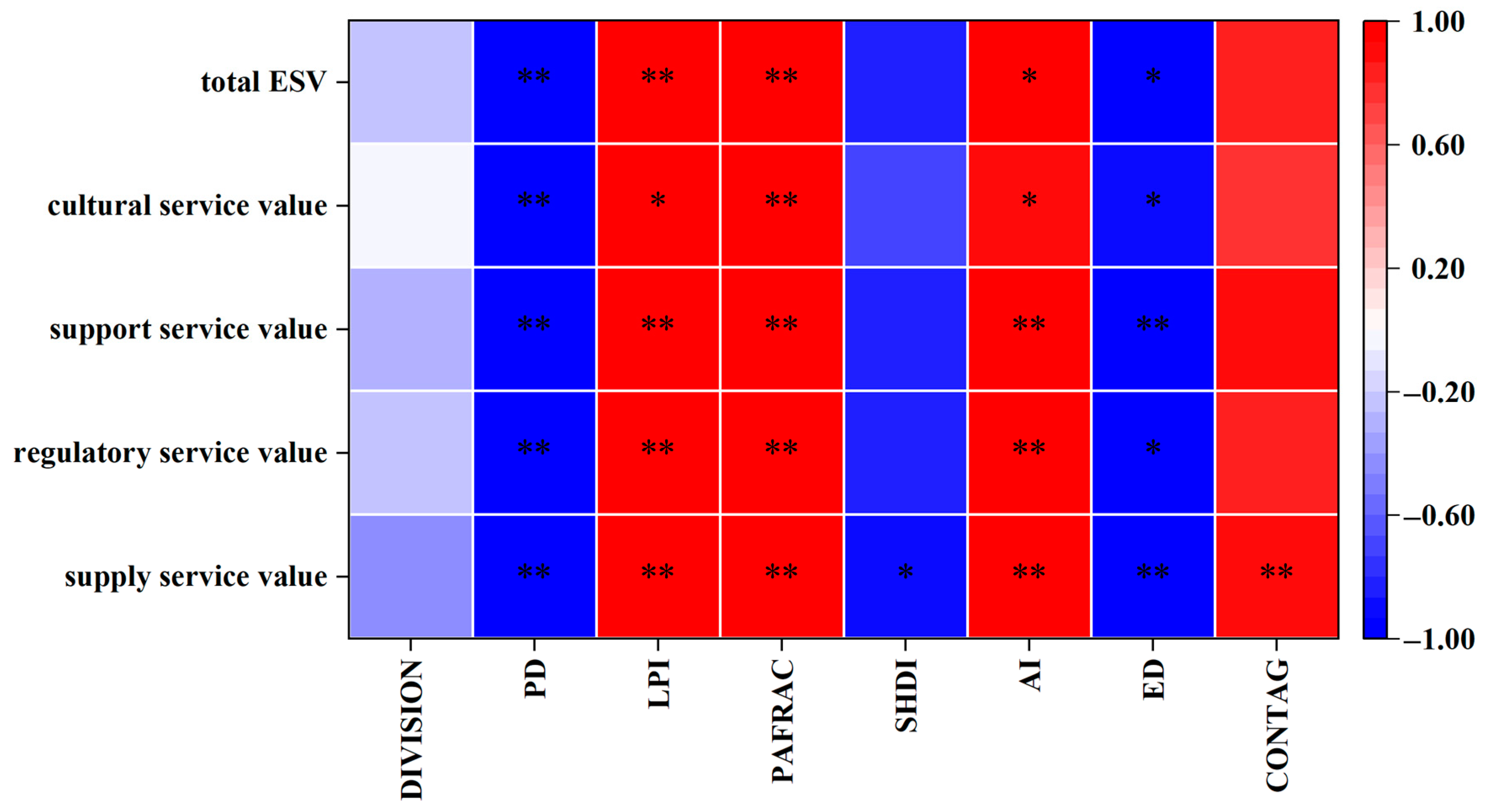
83], the PD and ED in the Yihe River Basin have a negative impact on the total ESV during the research period. Moreover, the LPI, PAFRAC, and aggregation degree have a positive impact on the total ESV. Due to population growth and urbanization, the transformation of landscape patterns in this region is primarily driven by human activities [84]. Therefore, across the period, human activities remarkably shape the connection between landscape patterns and ESVs.
In scrutinizing the relationships between landscape pattern indexes and the ESV, a substantial portion of existing research in the literature overlooks the spatial heterogeneity inherent in landscape pattern variables [
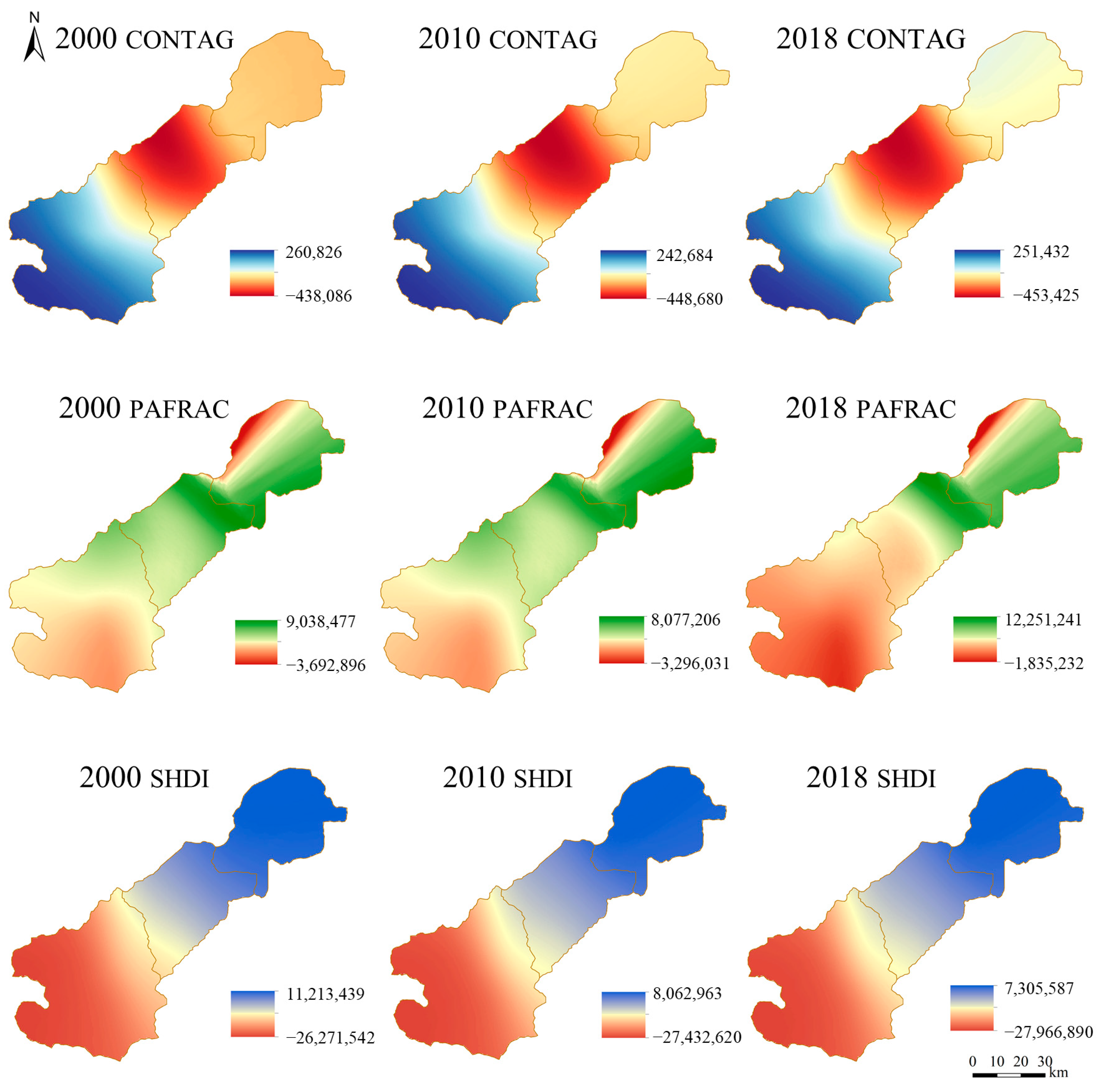
44]. Consequently, it falls short in capturing the influence of spatial alterations in landscape pattern indexes on the ESV. Our study found that in terms of spatial variations, the CONTAG, PAFRAC, and SHDI were noticeably correlated with the ESV. This correlation varies considerably across different regions and shows spatial heterogeneity characteristics. The CONTAG index is positively correlated with the ESV upstream, but negatively midstream and downstream. CONTAG reflects the agglomeration degree of patch types. In the upper basin, forestland prevails as the dominant landscape type, and its clustered distribution contributes positively to enhancing the ESV. Conversely, in the lower basin, the clustering of landscape types associated with lower ESVs hinders the improvement of the overall ESV. The SHDI is negatively correlated with ESVs upstream, but positively midstream and downstream. In the upper basin, the ecosystem thrives, whereas in the middle and lower reaches, it exhibits a comparatively delicate condition. The relationships between the SHDI and ESV reveals that in ecologically complex regions, the higher the SHDI value is, the higher the ESV; conversely, in more fragile ecological areas, the higher the SHDI is, the lower the ESV. The PAFRAC exhibits a positive correlation with ESVs for the most part. The correlation is in agreement with the result for the temporal change, which shows that the PAFRAC has a positive impact on the total ESV.

4.3. Limitations and Implications

This study employed a Pearson correlation analysis to quantify the relationship in temporal changes between ESV and landscape patterns. The geographically weighted regression model was utilized to assess the spatial non-stationarity of the impact of landscape patterns on ESV. Nevertheless, our research has certain limitations. ESV is influenced by a myriad of factors, characterized by complex interdependencies that pose challenges in isolating the singular impact of any one factor without considering others. Due to constraints in data availability, this study focused exclusively on the association between changes in landscape patterns and ESV, lacking a quantitative analysis of the driving mechanisms behind these landscape pattern and ESV changes. Furthermore, the internal dynamics between landscape patterns and ESV were not extensively explored in this study. Future research endeavors could benefit from more sophisticated quantitative methods, considering both natural geographical factors and socio-cultural elements, to further elucidate the intricate relationships among ESV, ecological changes, and landscape patterns. Moreover, the association between landscape pattern indexes and ESV exhibits temporal and spatial inconsistencies in most instances, suggesting a spatiotemporal scale effect in their relationship. The mechanism underlying this spatiotemporal scale effect warrants further exploration in future studies.
Owing to continuous increase in construction land for tourism and urban development in the Yihe River Basin, forest land and other natural landscapes are occupied, which destroys the integrity of the original landscape. The ecological condition within the Yihe River Basin has not witnessed a substantial enhancement. Persistent issues such as altered landscape patterns stemming from changes in land use, diminished forested areas, the expansion of construction zones, and the heightened fragmentation of the landscape persist in a grave manner. Because the original landscape has been transformed into landscape types with a minute or negative ESV per unit area, the ESV has ultimately decreased. The local government consider spatial variations in landscape patterns and ESV holistically in the Yihe River Basin, establish corresponding ecological compensation mechanisms, and carry out regional coordination efforts to support sustainable development. While undergoing ecological protection and economic development in the Yihe River Basin, the protection of green land should be strengthened, the fragmentation of landscape patterns decreased, and the connectivity of the overall landscape pattern in the region enhanced to achieve the reasonable allocation and sustainable development of regional resources. Moreover, increasing the areas of forest land and water area that can provide a higher ESV through policy restriction and economic adjustment remains urgent. These measures include implementing ecological management, constructing scientific and perfect agricultural development pattern, and lowering the landscape fragmentation to further improve land use efficiency.

5. Conclusions

Forestland is the landscape with the greatest dominance. Apart from constructed land, all other types have experienced a decline in area, with the most notable change occurring in construction land.
The fragmentation of the overall landscape has increased, and the landscape diversity and richness have also increased. The aggregation of the landscape shows a downward trend.
Throughout the entire study period, the overall ESV gradually decreased, and the land cover type with the greatest contribution to the ESV is forestland.
In terms of temporal changes, the PD and ED of the overall area are significantly negatively correlated with the total ESVs. The LPI, PAFRAC, and aggregation are significantly positively correlated with the total ESVs.
In terms of spatial variations, the CONTAG, PAFRAC, and SHDI were noticeably correlated with the ESVs. The CONTAG is positively correlated with ESVs upstream, but negatively midstream and downstream. The SHDI is negatively correlated with ESVs upstream, but positively midstream and downstream. The PAFRAC, for the most part, exhibits a positive correlation with ESVs.
The association between landscape pattern indexes and the ESV exhibits temporal and spatial inconsistencies in most instances, suggesting a spatiotemporal scale effect in their relationship. Future investigations should delve into the driving mechanisms behind spatiotemporal changes in landscape patterns, ESV, and their interrelationships.

Author Contributions

Conceptualization, L.L. and H.W.; Formal analysis, Q.H.; Funding acquisition, L.L.; Methodology, Q.H.; Writing—original draft, Q.H.; Writing—review and editing, H.W. and X.W. All authors have read and agreed to the published version of the manuscript.

Funding

This research was funded by the Key project of Henan Provincial Science and Technology R&D Plan Joint Fund (225200810045) and National Natural Science Foundation of China (41901259).

Institutional Review Board Statement

Not applicable.

Informed Consent Statement

Not applicable.

Data Availability Statement

The data presented in this study are available on request from the corresponding author.

Conflicts of Interest

Author Xiaoli Wu was employed by the Henan Institute of Geophysical Spatial Information Co., Ltd. The remaining authors declare that the research was conducted in the absence of any commercial or financial relationships that could be construed as a potential conflict of interest.

References

  1. OuYang, Z.; Wang, X.; Miao, H. A Primary Study on Chinese Terrestrial Ecosystem Services and Their Ecological-Economic Values. Acta Ecol. Sin. 1999, 19, 607–613. (In Chinese) [Google Scholar]
  2. Millennium Ecosystem Assessment (MEA). Ecosystems and Human Well-Being: Synthesis; Island Press: Washington, DC, USA, 2005. [Google Scholar]
  3. Zhang, L.; Li, L.; Ma, D.; Zhang, P. Landscape pattern and ecosystem service value response: Taking Qianyang County as an example. Northwest Geol. 2022, 55, 274–283. (In Chinese) [Google Scholar]
  4. Su, C.; Fu, B. Discussion on links among landscape pattern, ecological precess, and ecosystem services. Chin. J. Nat. 2012, 34, 277–283. (In Chinese) [Google Scholar]
  5. Zhao, Q.; Wen, Z.; Chen, S.; Ding, S.; Zhang, M. Quantifying Land Use/Land Cover and Landscape Pattern Changes and Impacts on Ecosystem Services. Int. J. Environ. Res. Public Health 2020, 17, 126. [Google Scholar] [CrossRef]
  6. Estoque, R.C.; Murayama, Y. Quantifying landscape pattern and ecosystem service value changes in four rapidly urbanizing hill stations of Southeast Asia. Landsc. Ecol. 2016, 31, 1481–1507. [Google Scholar] [CrossRef]
  7. Šebelíková, L.; Csicsek, G.; Kirmer, A.; Vítovcová, K.; Ortmann-Ajkai, A.; Prach, K.; Řehounková, K. Spontaneous revegetation versus forestry reclamation—Vegetation development in coal mining spoil heaps across Central Europe. Land Degrad. Dev. 2018, 30, 3. [Google Scholar] [CrossRef]
  8. Kolář, V.; Tichánek, F.; Tropek, R. Evidence-Based Restoration of Freshwater Biodiversity after Mining: Experience from Central European Spoil Heaps. J. Appl. Ecol. 2021, 58, 1921–1932. [Google Scholar] [CrossRef]
  9. Dong, X.B.; Wang, X.W.; Wei, H.J.; Fu, B.J.; Wang, J.J.; Uriarte-Ruiz, M. Trade-offs between local farmers’ demand for ecosystem services and ecological restoration of the Loess Plateau, China. Ecosyst. Serv. 2021, 49, 101295. [Google Scholar] [CrossRef]
  10. Wei, H.; Xue, D.; Huang, J.; Liu, M.; Li, L. Identification of Coupling Relationship between Ecosystem Services and Urbanization for Supporting Ecological Management: A Case Study on Areas along the Yellow River of Henan Province. Remote Sens. 2022, 14, 2277. [Google Scholar] [CrossRef]
  11. Ran, P.; Hu, S.; Frazier, A.E.; Yang, S.; Song, X.; Qu, S. The Dynamic Relationships between Landscape Structure and Ecosystem Services: An Empirical Analysis from the Wuhan Metropolitan Area, China. J. Environ. Manag. 2023, 325, 116575. [Google Scholar] [CrossRef]
  12. Haines-Young, R.; Chopping, M. Quantifying landscape structure: A review of landscape indices and their application to forested landscapes. Prog. Phys. Geogr. 1996, 20, 418–445. [Google Scholar] [CrossRef]
  13. Liu, M.; Wei, H.; Dong, X.; Wang, X.-C.; Zhao, B.; Zhang, Y. Integrating Land Use, Ecosystem Service, and Human Well-Being: A Systematic Review. Sustainability 2022, 14, 6926. [Google Scholar] [CrossRef]
  14. Yu, C.; Li, L.; Wei, H. Coupling Landscape Connectedness, Ecosystem Service Value, and Resident Welfare in Xining City, Western China. Systems 2023, 11, 512. [Google Scholar] [CrossRef]
  15. Zhang, X.; Li, H.; Xia, H.; Tian, G.; Yin, Y.; Lei, Y.; Kim, G. The Ecosystem Services Value Change and Its Driving Forces Responding to Spatio-Temporal Process of Landscape Pattern in the Co-Urbanized Area. Land 2021, 10, 1043. [Google Scholar] [CrossRef]
  16. Duarte, G.T.; Santos, P.M.; Cornelissen, T.G.; Ribeiro, M.C.; Paglia, A.P. The effects of landscape patterns on ecosystem services: Meta-analyses of landscape services. Landsc. Ecol. 2018, 33, 1247–1257. [Google Scholar] [CrossRef]
  17. Feng, J.; Guo, L.; Li, X. Temporal and Spatial Variations of Land Uses and Their Influences on Ecosystem Service Function Values in Hanzhong City. Res. Soil Water Conserv. 2020, 27, 275–282. (In Chinese) [Google Scholar]
  18. Qin, Y.L.; Shi, P.; He, W.H.; Huo, C.P.; Li, P.; Li, Z.B.; Yang, S.T.; Feng, Z.H. Influence of urbanization on landscape pattern and ecosystem service value in Xi’an City. Acta Ecol. Sin. 2020, 40, 8239–8250. (In Chinese) [Google Scholar]
  19. Mcdonnell, M.J.; Pickett, S.T.A. Ecosystem structure and function along urban–rural gradients: An unexploited opportunity for ecology. Ecology 1990, 71, 1232–1237. [Google Scholar] [CrossRef]
  20. Kremer, P.; Hamstead, Z.A.; Mcphearson, T. The value of urban ecosystem services in New York City: A spatially explicit multicriteria analysis of landscape scale valuation scenarios. Environ. Sci. Policy 2016, 62, 57–68. [Google Scholar] [CrossRef]
  21. Wang, H.; Zhang, M.; Wang, C.; Wang, K.; Wang, C.; Li, Y.; Bai, X.; Zhou, Y. Spatial and Temporal Changes of Landscape Patterns and Their Effects on Ecosystem Services in the Huaihe River Basin, China. Land 2022, 11, 513. [Google Scholar] [CrossRef]
  22. Zhao, J.; Liu, S.; Wang, Z.; Gao, H.; Feng, S.; Wei, B.; Hou, Z.; Xiao, F.; Jing, L.; Liao, X. The Impact of Land Use and Landscape Pattern on Ecosystem Services in the Dongting Lake Region, China. Remote Sens. 2023, 15, 2228. [Google Scholar] [CrossRef]
  23. Ma, G.Q.; Xiao, J.P.; Li, Q.J.; Zhang, L.X.; An, B.; Sun, G.J.; Cheng, H.; Tang, J.Q.; Li, H. Impact of the evolution of Plateau Lake landscape pattern on ecosystem service value in the Pearl River basin: A case study of Yilong Lake Basin in Yunnan Province, China. Acta Geophys. 2023, 71, 1391–1407. [Google Scholar] [CrossRef]
  24. Yun, J.; Liu, H.; Xu, Z.; Cao, X.; Ma, L.; Wen, L.; Zhuo, Y.; Wang, L. Assessing Changes in the Landscape Pattern of Wetlands and Its Impact on the Value of Wetland Ecosystem Services in the Yellow River Basin, Inner Mongolia. Sustainability 2022, 14, 6328. [Google Scholar] [CrossRef]
  25. Meng, L.; Dong, J. LUCC and Ecosystem Service Value Assessment for Wetlands: A Case Study in Nansi Lake, China. Water 2019, 11, 1597. [Google Scholar] [CrossRef]
  26. Liu, J.; Chen, S.; Xia, T.; Wang, Q. Analysis on Changes of Wetland Landscape in Yellow River Delta and Influences on Ecosystem Services. Adv. Mar. Sci. 2008, 26, 417–477. [Google Scholar]
  27. Cai, G.; Lin, Y.; Zhang, F.; Zhang, S.; Wen, L.; Li, B. Response of Ecosystem Service Value to Landscape Pattern Changes under Low-Carbon Scenario: A Case Study of Fujian Coastal Areas. Land 2022, 11, 2333. [Google Scholar] [CrossRef]
  28. Guo, M.; Shu, S.; Ma, S.; Wang, L. Using high-resolution remote sensing images to explore the spatial relationship between landscape patterns and ecosystem service values in regions of urbanization. Environ. Sci. Pollut. Res. 2021, 28, 56139–56151. [Google Scholar] [CrossRef]
  29. Hu, Y.; Chen, D.; Fan, J.; Shi, Z. Evolution of landscape pattern around Taihu Lake and its influence on ecosystem services. Urban Probl. 2021, 4, 95–103. [Google Scholar]
  30. Fahrig, L. Effects of Habitat Fragmentation on Biodiversity. Annu. Rev. Ecol. Evol. Syst. 2003, 34, 487–515. [Google Scholar] [CrossRef]
  31. Asher, S.; Garg, T.; Novosad, P. The Ecological Impact of Transportation Infrastructure. Econ. J. 2020, 130, 1173–1199. [Google Scholar] [CrossRef]
  32. Ricketts, T.H.; Daily, G.C.; Ehrlich, P.R.; Michener, C.D. Economic Value of Tropical Forest to Coffee Production. Proc. Natl. Acad. Sci. USA 2004, 101, 12579–12582. [Google Scholar] [CrossRef] [PubMed]
  33. Baudron, F.; Dilla, A.M.; Tirfessa, D.; Argaw, M. Impact of farmland exclosure on the productivity and sustainability of a mixed crop-livestock system in the Central Rift Valley of Ethiopia. Agric. Ecosyst. Environ. 2015, 207, 109–118. [Google Scholar] [CrossRef]
  34. Kremen, C.; Williams, N.M.; Thorp, R.W.; Toyama, N. Crop Pollination from Native Bees at Risk from Agricultural Intensification. Proc. Natl. Acad. Sci. USA 2002, 99, 16812–16816. [Google Scholar] [CrossRef] [PubMed]
  35. Xiong, Y.; Zhang, A.; Liu, M.; Li, H. Effects of citrus orchard expansion on ecosystem services and landscape pattern: A case study of Xinfeng County, Jiangxi Province, China. Acta Ecol. Sin. 2022, 42, 7845–7857. [Google Scholar]
  36. Vigl, L.E.; Schirpke, U.; Tasser, E.; Tappeiner, U. Linking long-term landscape dynamics to the multiple interactions among ecosystem services in the European Alps. J. Landsc. Ecol. 2016, 31, 1903–1918. [Google Scholar] [CrossRef]
  37. Tran, D.X.; Pearson, D.; Palmer, A.; Lowry, J.; Gray, D.; Dominati, E.J. Quantifying spatial non-stationarity in the relationship between landscape structure and the provision of ecosystem services: An example in the New Zealand hill country. Sci. Total Environ. 2022, 808, 152126. [Google Scholar] [CrossRef]
  38. Cao, J.; Zhang, Z.; Cui, F.; Chen, S.; Yang, Y.; Kuang, T.; Chen, Y. Response of ecosystem services to landscape pattern changes in the new york bay area from 1996 to 2015. World Reg. Stud. 2021, 30, 826–838. [Google Scholar]
  39. Tong, C.; Tong, Y.; Li, J.; Zhu, Z.; Zhou, Y. The effects of landscape pattern change on ecosystem service values in the Zhoushan Archipelago. J. Mar. Sci. 2019, 37, 40–51. [Google Scholar]
  40. Xu, J.; Fan, F.; Liu, Y.; Chen, J.; Wei, J. Response of ecosystem services to landscape pattern and its changes in Wenchuan County, Sichuan Province. Acta Ecol. Sin. 2020, 40, 4724–4736. [Google Scholar]
  41. Mitchell, M.G.E.; Bennett, E.M.; Gonzalez, A. Strong and nonlinear effects of fragmentation on ecosystem service provision at multiple scales. Environ. Res. Lett. 2015, 10, 094014. [Google Scholar] [CrossRef]
  42. Grêt-Regamey, A.; Rabe, S.E.; Crespo, R.; Lautenbach, S.; Ryffel, A.; Schlup, B. On the importance of non-linear relationships between landscape patterns and the sustainable provision of ecosystem services. Landsc. Ecol. 2014, 29, 201–212. [Google Scholar] [CrossRef]
  43. Zheng, B.F.; Huang, Q.Y.; Tao, L.; Xie, Z.Y.; Ai, B.; Zhu, Y.H.; Zhu, J.Q. Landscape pattern change and its impacts on the ecosystem services value in southern Jiangxi Province. Acta Ecol. Sin. 2021, 41, 5940–5949. [Google Scholar]
  44. Wen, H.; Li, R. Temporal and spatial variation of ecosystem service value and its response to landscape pattern change in Guizhou Province, China. Chin. J. Appl. Ecol. 2022, 33, 3057–3086. (In Chinese) [Google Scholar]
  45. Liu, Y.; Long, H. Study on spatial-temporal patterns of land use transition and its impact on ecological service function of the Middle of Yangtze River Economic Belt. Econ. Geogr. 2017, 37, 161–170. [Google Scholar]
  46. Liu, Y.; Bi, J.; Lü, J.S. Trade-off and synergy relationships of ecosystem services and the driving forces: A case study of the Taihu Basin, Jiangsu Province. Acta Ecol. Sin. 2019, 39, 7067–7078. (In Chinese) [Google Scholar]
  47. Liu, L.; Chen, X.; Chen, W.; Ye, X. Identifying the Impact of Landscape Pattern on Ecosystem Services in the Middle Reaches of the Yangtze River Urban Agglomerations, China. Int. J. Environ. Res. Public Health 2020, 17, 5063. [Google Scholar] [CrossRef] [PubMed]
  48. Guo, S.; Wu, C.; Wang, Y.; Qiu, G.; Zhu, D.; Niu, Q.; Qin, L. Threshold effect of ecosystem services in response to climate change, human activity and landscape pattern in the upper and middle Yellow River of China. Ecol. Indic. 2022, 136, 108603. [Google Scholar] [CrossRef]
  49. Lyu, R.; Zhao, W.; Tian, X.; Zhang, J. Non-linearity impacts of landscape pattern on ecosystem services and their trade-offs: A case study in the City Belt along the Yellow River in Ningxia, China. Ecol. Indic. 2022, 136, 108608. [Google Scholar] [CrossRef]
  50. Zhao, L.; Yu, W.; Meng, P.; Zhang, J.; Zhang, J. InVEST model analysis of the impacts of land use change on landscape pattern and habitat quality in the Xiaolangdi Reservoir area of the Yellow River basin, China. Land Degrad. Dev. 2022, 33, 2870–2884. [Google Scholar] [CrossRef]
  51. Shengyan, D.; Fude, S.; Lexiang, Q.; Xinxiang, C.; Shuang, L.; Haomin, L. Forest landscape patterns dynamics of Yihe-Luohe river basin. J. Geogr. Sci. 2003, 13, 153–162. [Google Scholar] [CrossRef]
  52. Meng, Q.; Zhang, L.; Wei, H.; Cai, E.; Xue, D.; Liu, M. Linking Ecosystem Service Supply–Demand Risks and Regional Spatial Management in the Yihe River Basin, Central China. Land 2021, 10, 843. [Google Scholar] [CrossRef]
  53. Wei, H.; Han, Q.; Yang, Y.; Li, L.; Liu, M. Spatial Heterogeneity of Watershed Ecosystem Health and Identification of Its Influencing Factors in a Mountain–Hill–Plain Region, Henan Province, China. Remote Sens. 2023, 15, 3751. [Google Scholar] [CrossRef]
  54. Liu, J.; Kuang, W.; Zhang, Z.; Xu, X.; Qin, Y.; Ning, J.; Zhou, W.; Zhang, S.; Li, R.; Yan, C.; et al. Spatiotemporal characteristics, patterns, and causes of land-use changes in China since the late 1980s. J. Geogr. Sci. 2014, 24, 195–210. [Google Scholar] [CrossRef]
  55. Hou, B.; Wei, C.; Liu, X.; Meng, Y.; Li, X. Assessing Forest Landscape Stability through Automatic Identification of Landscape Pattern Evolution in Shanxi Province of China. Remote Sens. 2023, 15, 545. [Google Scholar] [CrossRef]
  56. Li, Y.; Geng, H. Evolution of Land Use Landscape Patterns in Karst Watersheds of Guizhou Plateau and Its Ecological Security Evaluation. Land 2022, 11, 2225. [Google Scholar] [CrossRef]
  57. Chen, D.; Zhang, F.; Jim, C.Y.; Bahtebay, J. Spatio-temporal evolution of landscape patterns in an oasis city. Environ. Sci. Pollut. Res. 2022, 30, 3872–3886. [Google Scholar] [CrossRef] [PubMed]
  58. Huang, F.; Ochoa, C.G.; Jarvis, W.T.; Zhong, R.; Guo, L. Evolution of landscape pattern and the association with ecosystem services in the Ili-Balkhash Basin. Environ. Monit. Assess. 2022, 194, 171. [Google Scholar] [CrossRef]
  59. Lan, Y.; Chen, J.; Yang, Y.; Ling, M.; You, H.; Han, X. Landscape Pattern and Ecological Risk Assessment in Guilin Based on Land Use Change. Int. J. Environ. Res. Public Health 2023, 20, 2045. [Google Scholar] [CrossRef]
  60. Pan, F.; Shu, N.; Wan, Q.; Huang, Q. Land Use Function Transition and Associated Ecosystem Service Value Effects Based on Production–Living–Ecological Space: A Case Study in the Three Gorges Reservoir Area. Land 2023, 12, 391. [Google Scholar] [CrossRef]
  61. Daily, G.C. Nature’s Services: Societal Dependence on Natural Ecosystems; Island Press: Washington, DC, USA, 1997; pp. 454–464. [Google Scholar]
  62. Costanza, R.; Arge, R.D.; Groot, R.D.; Farberk, S.; Grasso, M.; Hannon, B.; Limburg, K.; Naeem, S.; Paruelo, J.; Raskin, R.G.; et al. The value of the world’s ecosystem services and natural capital. Nature 1997, 25, 3–15. [Google Scholar] [CrossRef]
  63. Xie, G.; Zhang, C.; Zhen, L.; Zhang, L. Dynamic changes in the value of China’s ecosystem services. Ecosyst. Serv. 2017, 26, 146–154. (In Chinese) [Google Scholar] [CrossRef]
  64. Xie, G.; Zhen, L.; Lu, C.-X.; Xiao, Y.; Chen, C. Expert knowledge based valuation method of ecosystem services in China. J. Nat. Resour. 2008, 23, 911–919. (In Chinese) [Google Scholar]
  65. Xie, G.; Zhang, C.; Zhang, L.; Chen, W.; Li, S. Improvement of the evaluation method for ecosystem service value based on per unit area. J. Nat. Resour. 2015, 30, 1243–1254. (In Chinese) [Google Scholar]
  66. Li, X.; Zhu, Y.; Zhao, L.; Tian, J.; Li, J. Ecosystem services value change in Qinglong County from dynamically adjusted value coefficients. Chin. J. Eco-Agric. 2015, 23, 373–381. (In Chinese) [Google Scholar]
  67. Ji, Z.; Wei, H.; Xue, D.; Liu, M.; Cai, E.; Chen, W.; Feng, X.; Li, J.; Lu, J.; Guo, Y. Trade-Off and Projecting Effects of Land Use Change on Ecosystem Services under Different Policies Scenarios: A Case Study in Central China. Int. J. Environ. Res. Public Health 2021, 18, 3552. [Google Scholar] [CrossRef] [PubMed]
  68. Yang, X.; Qiu, X.; Xu, Y.; Zhu, F.; Liu, Y. Spatial heterogeneity and dynamic features of the ecosystem services influence on human wellbeing in the West Sichuan Mountain Areas. Acta Ecol. Sin. 2021, 41, 7555–7567. (In Chinese) [Google Scholar]
  69. Cao, X.; Liu, Z.; LI, S. Identification of key areas of ecological protection and restoration based on the pattern of ecological security: A case of Songyuan City, Jilin province. China Environ. Sci. 2022, 42, 2779–2787. [Google Scholar]
  70. Wu, J.; Li, Y. Variation of Landscape Pattern and Its Influences on Ecosystem Service in Value in Three Gorges Reservoir Area (Chongqing Section). J. Ecol. Rural Environ. 2018, 34, 308–317. [Google Scholar]
  71. Long, H.; Liu, Y.; Hou, X.; Li, T.; Li, Y. Effects of land use transitions due to rapid urbanization on ecosystem services: Implications for urban planning in the new developing area of China. Habitat Int. 2014, 44, 536–544. [Google Scholar] [CrossRef]
  72. Wu, C.; Chen, B.; Huang, X.; Dennis Wei, Y.H. Effect of land-use change and optimization on the ecosystem service values of Jiangsu province, China. Ecol. Indic. 2020, 117, 106507. [Google Scholar] [CrossRef]
  73. Guo, P.; Zhang, F.; Wang, H. The response of ecosystem service value to land use change in the middle and lower Yellow River: A case study of the Henan section. Ecol. Indic. 2022, 140, 109019. [Google Scholar] [CrossRef]
  74. Wang, L.; Zhang, Z.; Li, G.; Ma, F.; Chen, L. Landscape pattern change in Beijing fringe area and its impact on the ecosystem services: A case study in Niulanshan-Mapo town. Acta Ecol. Sin. 2018, 38, 750–759. (In Chinese) [Google Scholar]
  75. Cheng, L.; Li, F.; Deng, H.-F. Dynamics of land use and its ecosystem services in China’s megacities. Acta Ecol. Sin. 2011, 31, 6194–6203. [Google Scholar]
  76. Zou, Y.; Zhou, Z. Impact of landscape pattern change on ecosystem service value of Xi’an City, China. Chin. J. Appl. Ecol. 2017, 28, 2629–2639. [Google Scholar]
  77. Yu, Y.; Li, M.; Han, X.; Liu, H. Study on the Response of Ecosystem Service Value to the Evolution of Landscape Pattern in Border Areas—Taking Yanbian Korean Autonomous Prefecture as an Example. Res. Soil Water Conserv. 2021, 28, 315–322. (In Chinese) [Google Scholar]
  78. Zhang, M.Y.; Wang, K.L.; Liu, H.Y.; Chen, H.S.; Zhang, C.H.; Yue, Y.M. Responses of ecosystem service values to landscape pattern change in typical Karst area of northwest Guangxi, China. Chin. J. Appl. Ecol. 2010, 21, 1174–1179. [Google Scholar]
  79. Liu, Y.; Ren, Z.; Li, C. Response of ecosystem services value to the landscape patterns change in Qinling Mountains—A case of Shangluo city. J. Arid Land Resour. Environ. 2013, 27, 109–114. (In Chinese) [Google Scholar]
  80. Cen, X.; Wu, C.; Xing, X.; Fang, M.; Garang, Z.; Wu, Y. Coupling Intensive Land Use and Landscape Ecological Security for Urban Sustainability: An Integrated Socioeconomic Data and Spatial Metrics Analysis in Hangzhou City. Sustainability 2015, 7, 1459–1482. [Google Scholar] [CrossRef]
  81. Hou, L.; Wu, F.; Xie, X. The spatial characteristics and relationships between landscape pattern and ecosystem service value along an urban-rural gradient in Xi’an City, China. Ecol. Indic. 2020, 108, 105720. [Google Scholar] [CrossRef]
  82. Zhang, J.; Qu, M.; Wang, C.; Zhao, J.; Cao, Y. Quantifying landscape pattern and ecosystem service value changes: A case study at the county level in the Chinese Loess Plateau. Glob. Ecol. Conserv. 2020, 23, e1110. [Google Scholar] [CrossRef]
  83. Wang, B.; Luo, L. Service value of a bay city ecosystem based on green buildings and landscape pattern changes. Sustain. Comput. Inform. Syst. 2022, 35, 100758. [Google Scholar] [CrossRef]
  84. You, M.; Zou, Z.; Zhao, W.; Zhang, W.; Fu, C. Study on Land Use and Landscape Pattern Change in the Huaihe River Ecological and Economic Zone from 2000 to 2020. Heliyon 2023, 9, e07080. [Google Scholar] [CrossRef] [PubMed]
Figure 1. Location map of the Yihe River Basin.
Forests 14 02446 g001
Figure 2. Areas of various land cover types in the Yihe River Basin from 2000 to 2018.
Forests 14 02446 g002
Figure 3. Changes in various land cover types in the Yihe River Basin from 2000 to 2018.
Forests 14 02446 g003
Figure 4. Changes in landscape pattern indexes of various land cover types at the level of patch type in the Yihe River Basin from 2000 to 2018.
Forests 14 02446 g004
Figure 5. Spatial distribution of landscape pattern indexes in the Yihe River Basin.
Forests 14 02446 g005
Figure 6. Spatial distribution of ecosystem service value index in the Yihe River Basin.
Forests 14 02446 g006
Figure 7. Correlation between landscape pattern indexes and ecosystem service values in the Yihe River Basin. Note: * means significant at the level of 0.05; ** means significant at the level of 0.01.
Forests 14 02446 g007
Figure 8. Spatial distribution variations in the correlations between the three landscape pattern indexes and ESVs.
Forests 14 02446 g008
Table 1. Landscape pattern index and connotation.
Landscape Pattern IndexConnotation
The level of patch type
Percentage of landscape (PLAND)The proportion of each landscape type to the total landscape area
Landscape shape index (LSI)The ratio of the total length of the landscape boundary to the square root of the total area
Patch density (PD)Number of patches per unit area in each landscape type
Patch cohesion index (COHESION)The aggregation degree of each landscape type
Mean patch size (MPS)The ratio of the total area of landscape types to the number of patches
The level of landscape scale
Landscape division index (DIVISION)Separation degree of individual distributions of different patches in the overall landscape
Patch density (PD)Number of patches per unit area in the overall landscape
Largest patch index (LPI)The ratio of the largest patch area to the total landscape area
Perimeter–area fractal dimension (PAFRAC)The non-integer dimension of the irregular geometric shape of the landscape
Aggregation index (AI)The aggregation degree of the overall landscape
Shannon diversity index (SHDI)The landscape heterogeneity, diversity, or unbalanced distribution of each patch type
Contagion index (CONTAG)The agglomeration degree or extension trend of each patch type
Edge density (ED)The edge length per unit area between a patch and adjacent heterogeneous patches
Table 2. Ecological service value coefficient per unit area of ecosystem in the Yihe River Basin (CNY/hm2).
First Class TypeSecond Class TypeCultivated LandForest LandGrasslandWater AreaConstruction LandUnused Land
Provisioning servicesFood production1625.68536.47699.04861.6115.6332.51
Raw material production634.014844.52585.24568.99065.03
Regulating servicesGas regulation1170.497022.932438.52829.1097.54
Climate regulation1576.916616.512536.063348.90211.34
Hydrological regulation1251.776649.022471.0330,513.98−12,223.85113.8
Waste disposal2259.692796.172145.924,141.32−4001.67422.68
Supporting servicesSoil conservation2389.756535.233641.52666.5331.26276.37
Maintaining biodiversity1658.197331.813040.025576.08547.1650.27
Cultural servicesProviding aesthetic landscape276.373381.411414.347218.0115.63390.16
Total 12,842.8645,714.0718,971.6673,724.5−15,615.892259.69
Table 3. Multicollinearity test of the independent variable of regression equation.
Model 1AICONTAGDIVISIONLPIPAFRACPDSHDIED
Variance inflation factor118.1197.1581124.003826.1641.037163.959126.24817,314.553
Model 2CONTAGPAFRACSHDI
Variance inflation factor118.1191.0042.248
Note: AI—Aggregation; CONTAG—Contagion index; DIVISION—Landscape division; LPI—Largest patch index; PAFRAC—Perimeter–area fractal dimension; PD—Patch density; SHDI—The Shannon diversity index; ED—Edge density.
Table 4. Comparison of goodness-of-fit test for OLS model and GWR model.
YearOLSGWR
Adjust R2AICcAdjust R2AICc
20000.303 26,973.2050.541 26,659.968
20100.319 26,956.1890.536 26,668.494
20180.333 26,949.8570.546 26,660.957
Note: OLS—Ordinary least squares; GWR—Geographically weighted regression; AICc—Corrected Akaike information criterion.
Table 5. Dynamic degrees of various land cover types in the Yihe River Basin from 2000 to 2018 (%).
PeriodsCultivated LandForest LandGrasslandWaterConstruction Land
2000–2005−0.110.00−0.010.281.00
2005–20100.02−0.06−0.51−4.153.35
2010–2015−0.24−0.02−0.02−0.031.81
2015–2018−0.07−0.010.000.790.83
2000–2018−0.10−0.02−0.15−0.992.05
Table 6. Landscape scale indexes in the Yihe River Basin from 2000 to 2018.
YearDIVISIONPDLPI/%PAFRACAISHDICONTAG/%ED/(m/hm2)
20000.85780.43229.37971.495296.94861.139463.743520.3044
20050.85870.432429.31891.493496.93341.144963.563320.4069
20100.85740.483329.22011.46796.8931.143863.570920.6753
20150.85860.509929.19241.459796.82031.158963.060321.1665
20180.85890.510329.18431.460696.82261.157563.099921.1475
Table 7. Ecosystem service values of various landscape types and total value in the Yihe River Basin from 2000 to 2018 (Unit: a hundred million CNY).
YearCultivated LandForest LandGrasslandWater AreaConstruction LandTotal Value
200022.8790.886.756.54−2.81124.23
200522.7590.866.756.63−2.95124.04
201022.7890.606.585.26−3.44121.78
201522.5090.606.575.25−3.76121.16
201822.4590.506.575.37−3.85121.04
Disclaimer/Publisher’s Note: The statements, opinions and data contained in all publications are solely those of the individual author(s) and contributor(s) and not of MDPI and/or the editor(s). MDPI and/or the editor(s) disclaim responsibility for any injury to people or property resulting from any ideas, methods, instructions or products referred to in the content.

