
Estimation of Carbon Stocks of Birch Forests on Abandoned Arable Lands in the Cis-Ural Using Unmanned Aerial Vehicle-Mounted LiDAR Camera

 ,
,  ,
,  and
and
Abstract
:1. Introduction
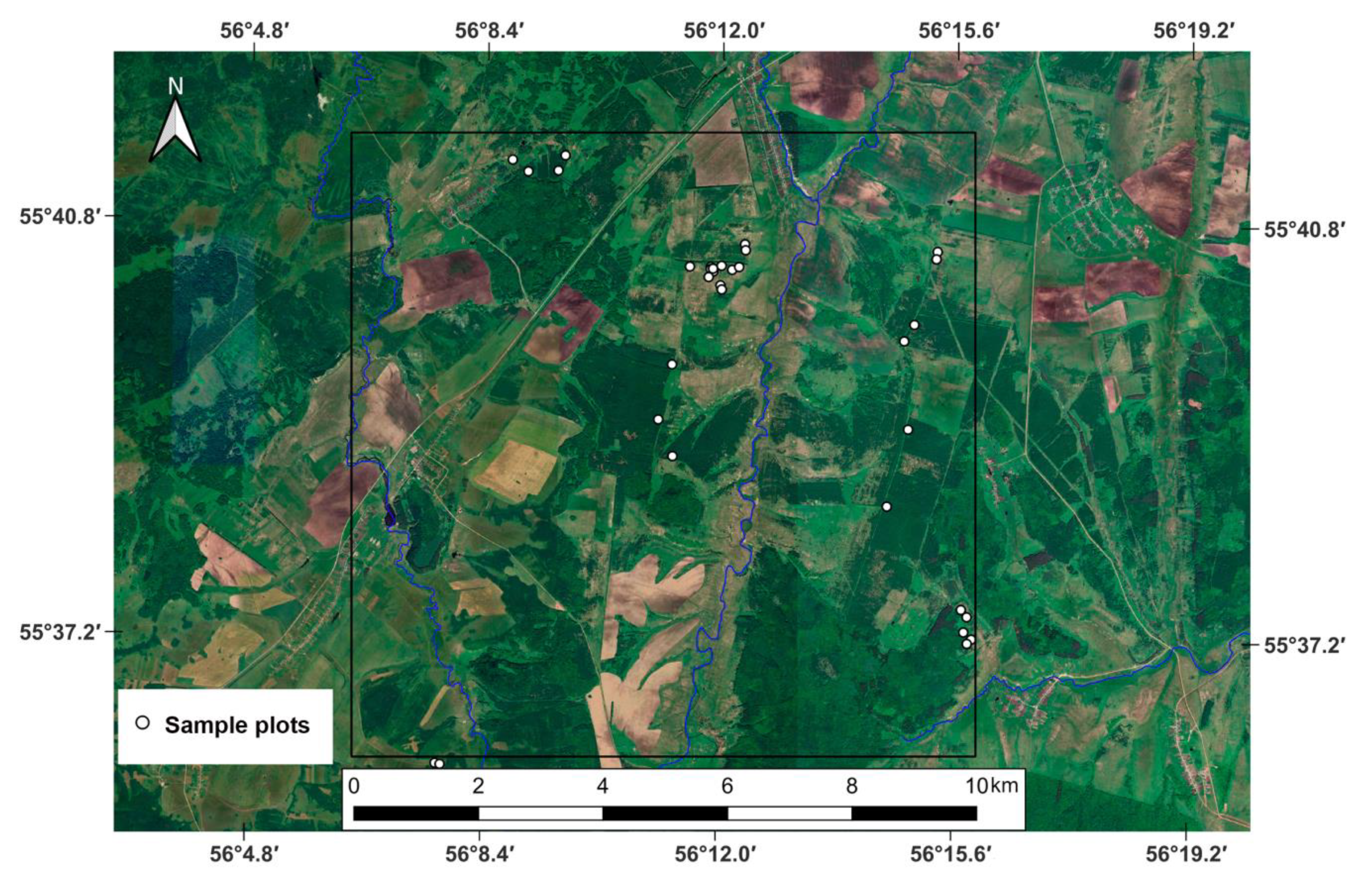
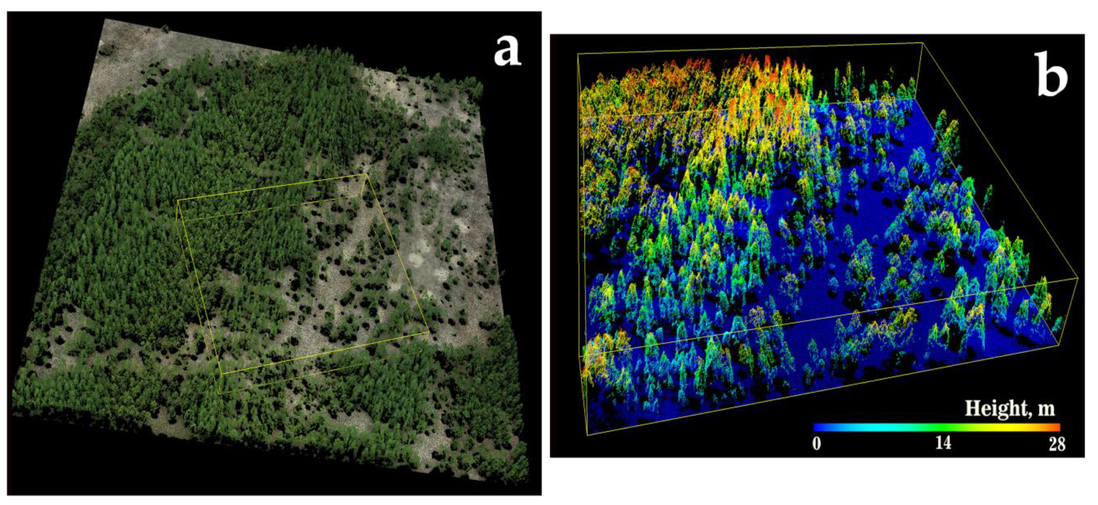
2. Materials and Methods
3. Results
4. Discussion
5. Conclusions
Author Contributions
Funding
Data Availability Statement
Conflicts of Interest
References
- MacDonald, D.; Crabtree, J.R.; Wiesinger, G.; Dax, T.; Stamou, N.; Fleury, P.; Gutiérrez-Lazpita, J.G.; Gibon, A. Agricultural abandonment in mountain areas of Europe: Environmental consequences and policy response. J. Environ. Manag. 2000, 59, 47–69. [Google Scholar] [CrossRef]
- Cramer, V.A.; Hobbs, R.J.; Standish, R.J. What’s new about old fields? Land abandonment and ecosystem assembly. Trends Ecol. Evol. 2008, 23, 104–112. [Google Scholar] [CrossRef]
- Bergen, K.M.; Zhao, T.; Kharuk, V.; Blam, Y.; Brown, D.G.; Peterson, L.K.; Miller, N. Changing regimes: Forested land cover dynamics in Central Siberia 1974 to 2001. Photogramm. Eng. Remote Sens. 2008, 74, 787–798. [Google Scholar] [CrossRef]
- Baumann, M.; Kuemmerle, T.; Elbakidze, M.; Ozdogan, M.; Radeloff, V.C.; Keuler, N.S.; Prishchepov, A.V.; Kruhlov, I.; Hostert, P. Patterns and drivers of post-socialist farmland abandonment in Western Ukraine. Land Use Policy 2011, 28, 552–562. [Google Scholar] [CrossRef]
- Hostert, P.; Kuemmerle, T.; Prishchepov, A.V.; Sieber, A.; Lambin, E.F.; Radeloff, V.C. Rapid land-use change after socio-economic disturbances: The collapse of the Soviet Union versus Chernobyl. Environ. Res. Lett. 2011, 6, 045201. [Google Scholar] [CrossRef]
- Tikkanen, O.P.; Chernyakova, I.; Heikkilä, R. Vanished villages—Imprint of traditional agriculture in forest landscape of western White Sea Karelia. Tr. Karel. Nauchnogo Tsentra RAN 2014, 6, 148–156. [Google Scholar]
- Levers, C.; Schneider, M.; Prishchepov, A.V.; Estel, S.; Kuemmerle, T. Spatial variation in determinants of agricultural land abandonment in Europe. Sci. Total Environ. 2018, 644, 95–111. [Google Scholar] [CrossRef]
- Crawford, C.L.; Yin, H.; Radeloff, V.C.; Wilcove, D.S. Rural land abandonment is too ephemeral to provide major benefits for biodiversity and climate. Sci. Adv. 2022, 8, eabm8999. [Google Scholar] [CrossRef]
- Campbell, J.E.; Lobell, D.B.; Field, C.B. Greater transportation energy and GHG offsets from bioelectricity than ethanol. Science 2009, 324, 1055–1057. [Google Scholar] [CrossRef]
- Gibbs, H.K.; Salmon, J.M. Mapping the world’s degraded lands. Appl. Geogr. 2015, 57, 12–21. [Google Scholar] [CrossRef]
- Lerman, Z.; Csaki, C.; Feder, G. Agriculture in Transition: Land Policies and Evolving Farm Structures in Post-Soviet Countries; Lexington Books: Lanham, MD, USA, 2004. [Google Scholar]
- Lyuri, D.I.; Goryachkin, S.V.; Karavaeva, N.A.; Denisenko, E.A.; Nefedova, T.G. Dynamics of Agricultural Land in Russia in the XX Century and Post-Agricultural Restoration of Vegetation and Soils; GEOS: Moskow, Russia, 2010; p. 416. [Google Scholar]
- Uzun, V.Y. “White spots” and unused agricultural land: What the agricultural census of 2016 showed. In Monitoring of the Economic Situation in Russia; Trends and Challenges of Socio-Economic Development; Gaidar Institute for Economic Policy and RANEPA: Moscow, Russia, 2017; Volume 21, pp. 14–21. [Google Scholar]
- Bai, W.; Mitchley, J.; Jiao, J. Soil seed bank and standing vegetation of abandoned croplands on Chinese Loess Plateau: Implications for restoration. Arid Land Res. Manag. 2010, 24, 98–116. [Google Scholar] [CrossRef]
- Anpilogova, D.; Pakina, A. Assessing ecosystem services of abandoned agricultural lands: A case study. One Ecosyst. 2022, 7, e77969. [Google Scholar] [CrossRef]
- Zhizhin, S.M.; Magasumova, A.G. Overgrowing of agricultural lands with tree and shrub vegetation in the zone of coniferous-broad-leaved forests of the Republic of Udmurtia. Mezhdunarodnyy Nauchno-Issledovatel’skiy Zhurnal (Int. Res. J.) 2021, 104, 149–153. [Google Scholar] [CrossRef]
- Shirokikh, P.S.; Martynenko, V.B.; Zverev, A.A.; Bikbaev, I.G.; Ibragimov, I.I.; Bikbaeva, G.G.; Karimova, L.D.; Baisheva, E.Z. Vegetation of abandoned fields in the Bashkir Cis-Urals. Tomsk. State Univ. J. Biol. 2017, 37, 66–104. [Google Scholar] [CrossRef]
- Hynynen, J.; Niemistö, P.; Viherä-Aarnio, A.; Brunner, A.; Hein, S.; Velling, P. Silviculture of birch (Betula pendula Roth and Betula pubescens Ehrh.) in northern Europe. Forestry 2010, 83, 103–119. [Google Scholar] [CrossRef]
- Zasada, M.; Bijak, S.; Bronisz, K.; Bronisz, A.; Gawęda, T. Biomass dynamics in young silver birch stands on post-agricultural lands in central Poland. Drew. Pract. Nauk. Doniesienia Komun. 2014, 57, 29–40. [Google Scholar] [CrossRef]
- Fedorov, N.; Shirokikh, P.; Zhigunova, S.; Baisheva, E.; Tuktamyshev, I.; Bikbaev, I.; Komissarov, M.; Zaitsev, G.; Giniyatullin, R.; Gabbasova, I.; et al. Dynamics of biomass and carbon stocks during reforestation on abandoned agricultural lands in Southern Ural region. Agriculture 2023, 13, 1427. [Google Scholar] [CrossRef]
- Johansson, T. Biomass equations for determining fractions of common and grey alders growing on abandoned farmland and some practical implications. Biomass Bioenergy 1999, 18, 147–159. [Google Scholar] [CrossRef]
- Beck, P.; Caudullo, G.; de Rigo, D.; Tinner, W. Betula pendula and Betula pubescens. In European Atlas of Forest Tree Species; San-Miguel-Ayanz, J., de Rigo, D., Caudullo, G., Houston Durrant, T., Mauri, A., Eds.; Publication Office of the European Union: Luxembourg, 2016; pp. 70–74. [Google Scholar]
- Jagodziński, A.M.; Zasada, M.; Bronisz, K.; Bronisz, A.; Bijak, S. Biomass conversion and expansion factors for a chronosequence of young naturally regenerated silver birch (Betula pendula Roth) stands growing on post-agricultural sites. For. Ecol. Manag. 2017, 384, 208–220. [Google Scholar] [CrossRef]
- Uri, V.; Varik, M.; Aosaar, J.; Kanal, A.; Kukumägi, M.; Lohmus, K. Biomass production and carbon sequestration in a fertile silver birch (Betula pendula Roth) forest chronosequence. For. Ecol. Manag. 2012, 267, 117–126. [Google Scholar] [CrossRef]
- Varik, M.; Kukumagi, M.; Aosaar, J.; Becker, H.; Ostonen, I.; Lohmus, K.; Uri, V. Carbon budgets in fertile silver birch (Betula pendula Roth) chronosequence stands. Ecol. Eng. 2015, 77, 284–296. [Google Scholar] [CrossRef]
- Jonczak, J.; Jankiewicz, U.; Kondras, M.; Kruczkowska, B.; Oktaba, L.; Oktaba, J.; Olejniczak, I.; Pawłowicz, E.; Polláková, N.; Raab, T.; et al. The influence of birch trees (Betula spp.) on soil environment—A review. For. Ecol. Manag. 2020, 477, 118486. [Google Scholar] [CrossRef]
- Rytter, R.M.; Rytter, L.; Hogbom, L. Carbon sequestration in willow (Salix s) plantations on former arable land estimated by repeated field sampling and C budget calculation. Biomass Bioenergy 2015, 83, 483–492. [Google Scholar] [CrossRef]
- Smith, J.O.; Smith, P.; Wattenbach, M.; Gottschalk, P.I.A.; Romanenkov, V.A.; Shevtsova, L.K.; Lisovoi, N.V. Projected changes in the organic carbon stocks of cropland mineral soils of European Russia and the Ukraine, 1990–2007. Glob. Chang. Biol. 2007, 13, 342–356. [Google Scholar] [CrossRef]
- Vuichard, N.; Ciais, P.; Wolf, A. Soil carbon sequestration or biofuel production: New land-use opportunities for mitigating climate over abandoned soviet farmlands. Environ. Sci. Technol. 2009, 43, 8678–8683. [Google Scholar] [CrossRef] [PubMed]
- Ryzhova, I.M.; Erokhova, A.A.; Podvezennaya, M.A. Alterations of the carbon storages in postagrogenic ecosystems due to natural reforestation in Kostroma oblast. Russ. For. Sci. 2015, 4, 307–317. [Google Scholar] [CrossRef]
- Gong, J.; Chen, L.; Fu, B.-J.; Huang, Y. Effect of land use on soil nutrients in the loess hilly area of the Loess Plateau, China. Land Degrad. Dev. 2006, 17, 453–465. [Google Scholar] [CrossRef]
- Yanagawa, A.; Tamura, K.; Fujimaki, H.; Asano, M.; Ose, K.; Higashi, T. Effects of crop abandonment and grazing exclusion on available soil water and other soil properties in a semi-arid Mongolian grassland. Soil Tillage Res. 2009, 105, 228–235. [Google Scholar] [CrossRef]
- Novara, A.; Gristina, L.; Sala, G.; Galati, A.; Crescimanno, M.; Cerdà, A.; Badalamenti, E.; La Mantia, T. Agricultural land abandonment in Mediterranean environment provides ecosystem services via soil carbon sequestration. Sci. Total Environ. 2017, 576, 420–429. [Google Scholar] [CrossRef]
- Bell, S.M.; Barriocanal, C.; Terrer, C.; Rosell-Melé, A. Management opportunities for soil carbon sequestration following agricultural land abandonment. Environ. Sci. Policy 2020, 108, 104–111. [Google Scholar] [CrossRef]
- Kurganova, I.; De Gerenyu, V.L.; Kuzyakov, Y. Large-scale carbon sequestration in post-agrogenic ecosystems in Russia and Kazakhstan. Catena 2015, 133, 461–466. [Google Scholar] [CrossRef]
- Kurganova, I.; Lopes de Gerenyu, V.; Six, J.; Kuzyakov, Y. Carbon cost of collective farming collapse in Russia. Glob. Chang. Biol. 2014, 20, 938–947. [Google Scholar] [CrossRef]
- Lal, R. Carbon sequestration. Philos. Trans. R. Soc. B Biol. Sci. 2008, 363, 815–830. [Google Scholar] [CrossRef]
- Bronisz, K.; Lauri, M. Mixed-effects generalized height–diameter model for young silver birch stands on post-agricultural lands. For. Ecol. Manag. 2020, 460, 117901. [Google Scholar] [CrossRef]
- Janus, J.; Piotr, B.; Bartosz, M.; Taszakowski, J.; Doroż, A. Long-term forest cover and height changes on abandoned agricultural land: An assessment based on historical stereometric images and airborne laser scanning data. Ecol. Indic. 2021, 120, 106904. [Google Scholar] [CrossRef]
- Sačkov, I.; Barka, I.; Bucha, T. Mapping aboveground woody biomass on abandoned agricultural land based on airborne laser scanning data. Remote Sens. 2020, 12, 4189. [Google Scholar] [CrossRef]
- Simard, M.; Pinto, N.; Fisher, J.B.; Baccini, A. Mapping forest canopy height globally with spaceborne lidar. J. Geohys. Res. Biogeosci. 2011, 116, 4021. [Google Scholar] [CrossRef]
- Ahmed, O.S.; Franklin, S.E.; Wulder, M.; White, J.C. Characterizing stand-level forest canopy cover and height using Landsat time series, samples of airborne LiDAR, and the Random Forest algorithm. ISPRS J. Photogramm. Remote Sens. 2015, 101, 89–101. [Google Scholar] [CrossRef]
- Caughlin, T.T.; Rifai, S.W.; Graves, S.J.; Asner, G.P. Integrating LiDAR-derived tree height and Landsat satellite reflectance to estimate forest regrowth in a tropical agricultural landscape. Remote Sens. Ecol. Conserv. 2016, 2, 190–203. [Google Scholar] [CrossRef]
- Guo, Q.; Su, Y.; Hu, T.; Zhao, X. An integrated UAV-borne lidar system for 3D habitat mapping in three forest ecosystems across China. Int. J. Remote Sens. 2017, 38, 2954–2972. [Google Scholar] [CrossRef]
- Ma, W.; Domke, G.M.; Woodall, C.W.; D’Amato, A.W. Contemporary forest carbon dynamics in the northern U.S. associated with land cover changes. Ecol. Ind. 2020, 110, 105901. [Google Scholar] [CrossRef]
- Luo, S.; Wang, C.; Xi, X.; Nie, S.; Fan, X.; Chen, H.; Zhou, G. Combining hyperspectral imagery and LiDAR pseudo-waveform for predicting crop LAI, canopy height and above-ground biomass. Ecol. Ind. 2019, 102, 801–812. [Google Scholar] [CrossRef]
- Kedrov, A.V. Laser Taxation of Forests with Lidar Technology. Available online: https://lpk-sibiri.ru/forest-management/lesoustrojstvo/lazernaya-taksacziya-lesov-s-tehnologiej-lidar (accessed on 18 July 2023).
- Nizametdinov, N.F.; Moiseev, P.A.; Vorobyov, I.B. Laser scanning and aerial photography with UAVs in studying the structure of forest-tundra stands in the Khibiny mountains. For. J. 2021, 4, 9–22. [Google Scholar] [CrossRef]
- Usoltsev, V.A.; Kovyazin, V.; Tsepordey, I.; Zalesov, S.; Chasovskikh, V. Allometric models of Picea spp. biomass for airborne laser sensing as related to climate variables. IOP Conf. Ser. Earth Environ. Sci. 2021, 806, 12033. [Google Scholar] [CrossRef]
- Sibona, E.; Vitali, A.; Meloni, F.; Caffo, L.; Dotta, A.; Lingua, E.; Garbarino, M. Direct measurement of tree height provides different results on the assessment of LiDAR accuracy. Forests 2016, 8, 7. [Google Scholar] [CrossRef]
- Chiappini, S.; Pierdicca, R.; Malandra, F.; Tonelli, E.; Savina, E.; Urbinati, M.C.; Vitali, A. Comparing Mobile Laser Scanner and manual measurements for dendrometric variables estimation in a black pine (Pinus nigra Arn.) plantation. Comput. Electron. Agric. 2022, 198, 107069. [Google Scholar] [CrossRef]
- Neuville, R.; Bates, J.S.; Jonard, F. Estimating forest structure from UAV-Mounted LiDAR point cloud using machine learning. Remote Sens. 2021, 13, 352. [Google Scholar] [CrossRef]
- Hyyppa, E.; Hyyppa, J.; Hakala, T.; Kukko, A.; Wulder, M.A.; White, J.C.; Kaartinen, H. Under-canopy UAV laser scanning for accurate forest field measurements. ISPRS J. Photogramm. Remote Sens. 2020, 164, 41–60. [Google Scholar] [CrossRef]
- Hyyppa, E.; Kukko, A.; Kaijaluoto, R.; White, J.C.; Wulder, M.A.; Pyorala, J.; Hyyppa, J. Accurate derivation of stem curve and volume using backpack mobile laser scanning. ISPRS J. Photogramm. Remote Sens. 2020, 161, 246–262. [Google Scholar] [CrossRef]
- Chen, S.; Liu, H.; Feng, Z.; Shen, C.; Chen, P. Applicability of personal laser scanning in forestry inventory. PLoS ONE 2019, 14, E0211392. [Google Scholar] [CrossRef]
- Luo, H.; Wang, L.; Wu, C.; Zhang, L. An improved method for impervious surface mapping incorporating LiDAR data and high-resolution imagery at different acquisition times. Remote Sens. 2018, 10, 1349. [Google Scholar] [CrossRef]
- Statgraphics Technologies. Statgraphics 19 Centurion. Software. 2020. Available online: https://www.statgraphics.com/ (accessed on 17 September 2023).
- Huang, S.; Titus, S.J.; Wiens, D.P. Comparison of nonlinear height-diameter functions for major Alberta tree species. Can. J. For. Res. 1992, 22, 1297–1307. [Google Scholar] [CrossRef]
- Ni-Meister, W.; Rojas, A.; Lee, S. Direct use of large-footprint lidar waveforms to estimate aboveground biomass. Remote Sens. Environ. 2022, 280, 113147. [Google Scholar] [CrossRef]
- Du, L.; Pang, Y.; Wang, Q.; Huang, C.; Bai, Y.; Chen, D.; Lu, W.; Kong, D. A LiDAR biomass index-based approach for tree- and plot-level biomass mapping over forest farms using 3D point clouds. Remote Sens. Environ. 2023, 290, 113543. [Google Scholar] [CrossRef]
- Niemistö, P. Infuence of initial spacing and row-to-row distance on the crown and branch properties and taper of silver birch (Betula pendula). Scand. J. For. Res. 1995, 10, 235–244. [Google Scholar] [CrossRef]
- Holiaka, D.; Kato, H.; Yoschenko, V.; Onda, Y.; Igarashi, Y.; Nanba, K.; Diachuk, P.; Holiaka, M.; Zadorozhniuk, R.; Kashparov, V.; et al. Scots pine stands biomass assessment using 3D data from unmanned aerial vehicle imagery in the Chernobyl Exclusion Zone. J. Environ. Manag. 2021, 295, 113319. [Google Scholar] [CrossRef]
- Fedorov, N.I.; Zharkikh, T.L.; Mikhailenko, O.I.; Bakirova, R.T.; Martynenko, V.B. Forecast changes in the productivity of plant communities in the Pre-Urals steppe site of Orenburg state nature reserve (Russia) in extreme drought conditions using NDVI. Nat. Conserv. Res. 2019, 4, 104–110. [Google Scholar] [CrossRef]
- Đomlija, P.; Bernat Gazibara, S.; Arbanas, Ž.; Mihalić Arbanas, S. Identification and mapping of soil erosion processes using the visual interpretation of LiDAR Imagery. ISPRS Int. J. Geo-Inf. 2019, 8, 438. [Google Scholar] [CrossRef]
- Eltner, A.; Baumgart, P. Accuracy constraints of terrestrial Lidar data for soil erosion measurement: Application to a Mediterranean field plot. Geomorphology 2015, 245, 243–254. [Google Scholar] [CrossRef]
- Campbell, M.J.; Eastburn, J.F.; Mistick, K.A.; Smith, A.M.; Stovall, A.E.L. Mapping individual tree and plot-level biomass using airborne and mobile lidar in piñon-juniper woodlands. Int. J. Appl. Earth. Obs. Geoinf. 2023, 118, 103232. [Google Scholar] [CrossRef]
- Huang, W.; Sun, G.; Dubayah, R.; Cook, B.; Montesano, P.; Ni, W.; Zhang, Z. Mapping biomass change after forest disturbance: Applying LiDAR footprint-derived models at key map scales. Remote Sens. Environ. 2013, 134, 319–332. [Google Scholar] [CrossRef]
- Barbosa, J.M.; Broadbent, E.N.; Bitencourt, M.D. Remote sensing of aboveground biomass in tropical secondary forests: A review. Int. J. For. Res. 2014, 2014, 715796. [Google Scholar] [CrossRef]
- Dalponte, M.; Jucker, T.; Liu, S.; Frizzera, L.; Gianelle, D. Characterizing forest carbon dynamics using multi-temporal lidar data. Remote Sens. Environ. 2019, 224, 412–420. [Google Scholar] [CrossRef]
- Le Toan, T.; Quegan, S.; Woodward, I.; Lomas, M.; Delbart, N.; Picard, G. Relating radar remote sensing of biomass to modelling of forest carbon budgets. Clim. Chang. 2004, 67, 379–402. [Google Scholar] [CrossRef]

| Stage of Reforestation | Trees Height, m | Age of Trees, Years | Diameter of Trunks, cm | Variant 1 (Projective Coverage, %) | Number of Plots Variant 1 | Variant 2 (Projective Coverage, %) | Number of Plots Variant 2 |
|---|---|---|---|---|---|---|---|
| I | 0.5–1.5 | 3–8 | – | 1–5 | 2 | 7–10 | – |
| II | 2–3 | 9–14 | 1–3 | 10–20 | 1 | 30–50 | 5 |
| III | 5–8 | 15–20 | 6–8 | 30–50 | 3 | 60–80 | 1 |
| IV | 9–14 | 20–25 | 10–14 | 50–60 | 4 | 75–90 | 3 |
| V | 15–18 | 25–30 | 16–20 | 50–60 | – | 75–90 | 6 |
| Stand Characteristics | Regression Model Equation | R | R2 | ESE |
|---|---|---|---|---|
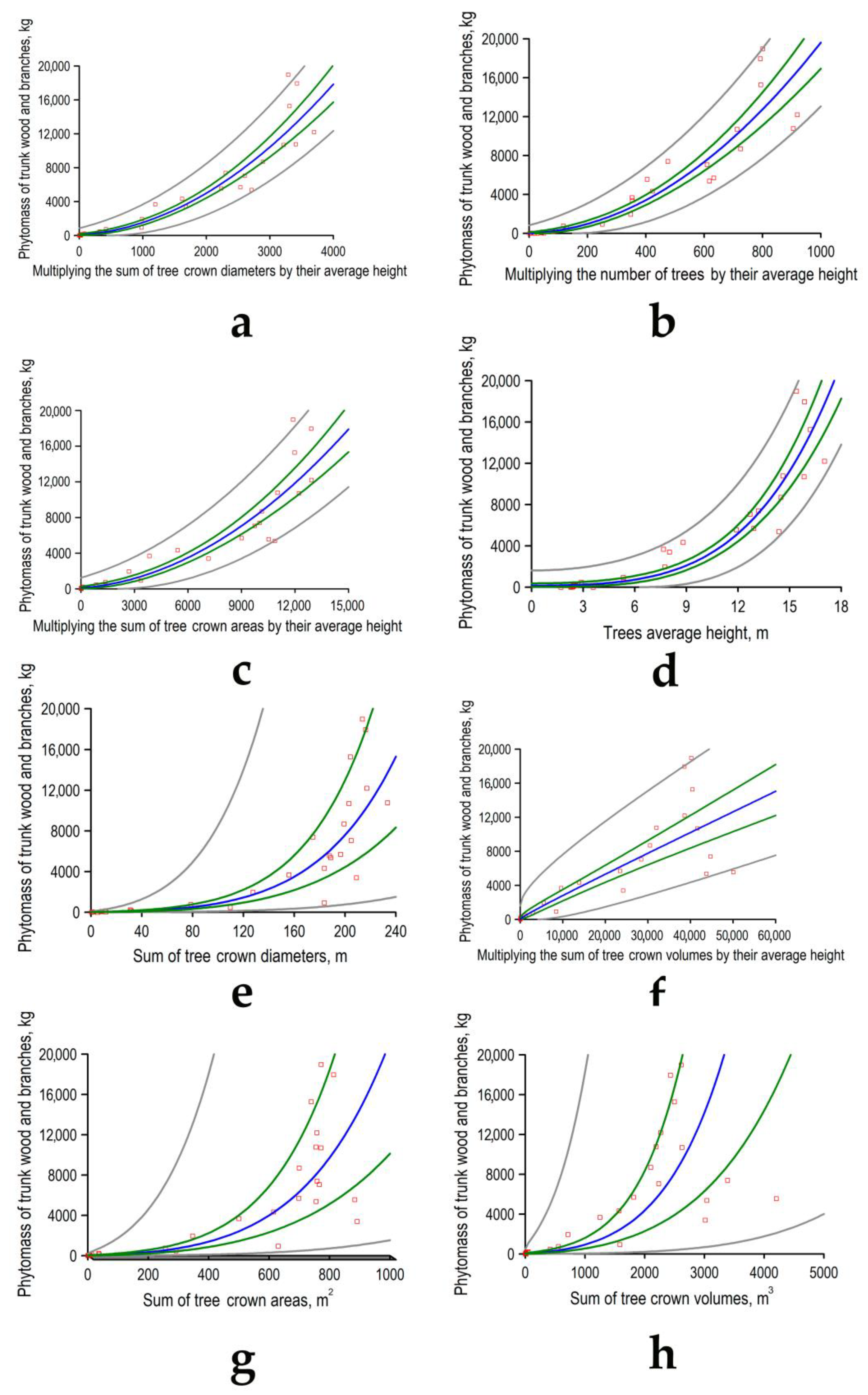
| Phytomass of stem wood with branches | ||||
| Multiplying the sum of tree crowns diameters by their average height | Square root-Y model: Y = (6.25464 + 0.0320395 × X)2 | 0.98 | 95.5 | 9.8 |
| Multiplying the number of trees by their average height | Square root-Y model: Y = (3.33595 + 0.1372 × X)2 | 0.97 | 94.4 | 10.9 |
| Multiplying the sum of tree crown area by their average height | Square root-Y model: Y = (7.46822 + 0.00848049 × X)2 | 0.97 | 93.5 | 11.7 |
| Trees average height | Square root-Y squared-X model: Y = (9.49088 + 0.430736 × X2)2 | 0.96 | 92.1 | 12.9 |
| Sum of trees crown diameters | Logarithmic-Y square root-X model: Y = exp(0.875185 + 0.576223 × √X) | 0.94 | 89.2 | 1.2 |
| Multiplying the sum of tree crown volumes by their average height | Double square root model: Y = (3.98812 + 0.486332 × √X)2 | 0.94 | 88.8 | 15.4 |
| Sum of tree crown areas | Logarithmic-Y square root-X model: Y = exp(1.64388 + 0.270862 × √X) | 0.92 | 84.0 | 1.5 |
| Sum of tree crown volumes | Logarithmic-Y square root-X model: Y = exp(2.16932 + 0.138317 × √X) | 0.88 | 78.0 | 1.7 |
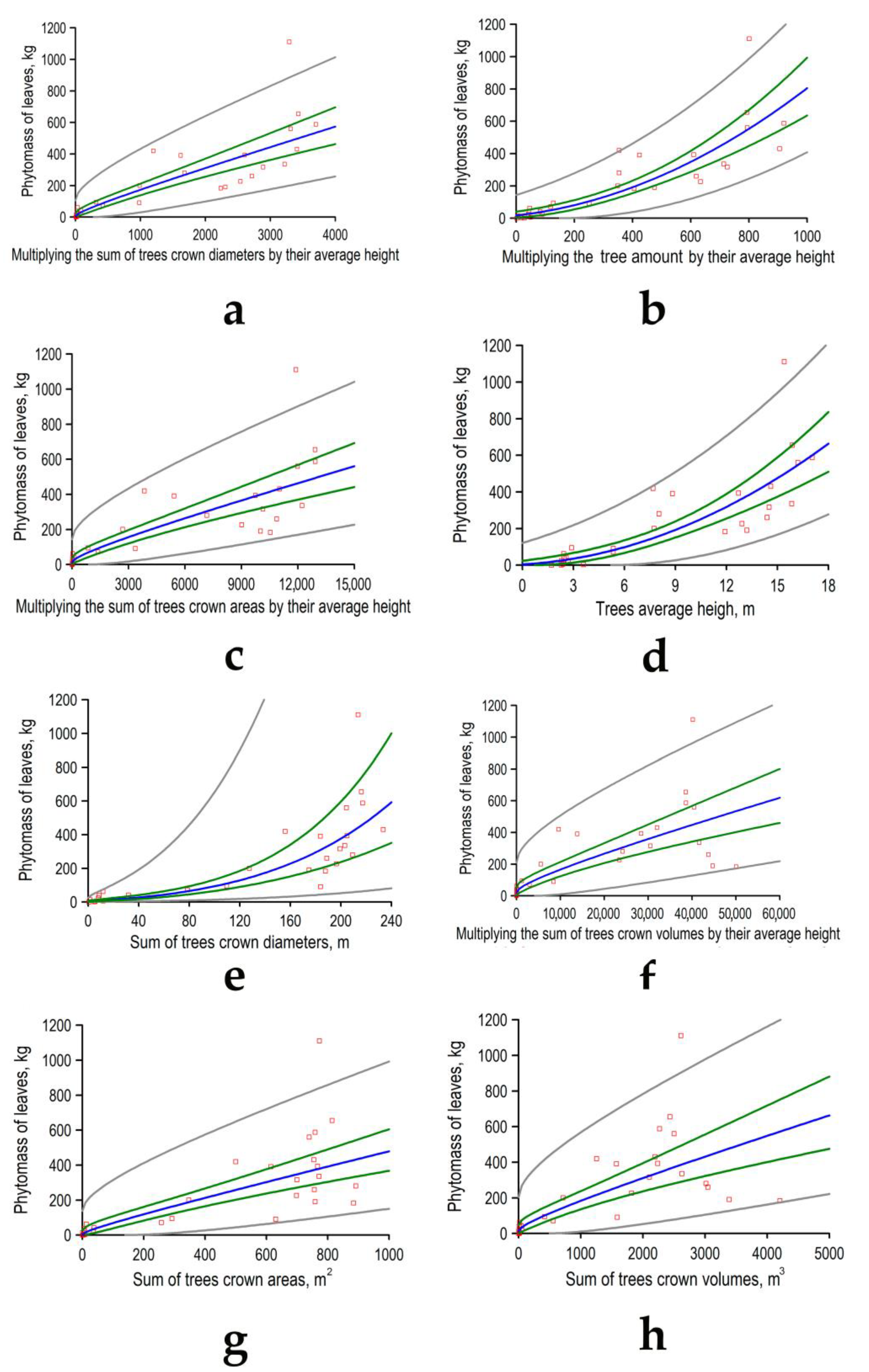
| Phytomass of leaves | ||||
| Multiplying the sum of tree crown diameters by their average height | Double square root model: Y = (1.98201 + 0.3495 × √X)2 | 0.92 | 85.4 | 3.4 |
| Multiplying the number of trees by their average height | Square root-Y model: Y = (3.38375 + 0.0254409 × X)2 | 0.92 | 84.4 | 3.5 |
| Sum of tree crown diameters | Logarithmic-Y square root-X model: Y = exp(0.656103 + 0.377484 × √X) | 0.91 | 83.6 | 1.0 |
| Multiplying the sum of tree crown areas by their average height | Double square root model: Y = (2.79809 + 0.172115 × √X)2 | 0.91 | 82.3 | 3.8 |
| Tree average height | Square root-Y model: Y = (1.32037 + 1.37447 × X)2 | 0.90 | 81.0 | 3.9 |
| Sum of tree crown areas | Double square root model: Y = (1.70192 + 0.641025 × √X)2 | 0.88 | 78.2 | 4.2 |
| Multiplying the sum of tree crown volumes by their average height | Double square root model: Y = (3.70018 + 0.0880252 × √X)2 | 0.87 | 76.0 | 4.4 |
| Sum of tree crown volumes | Double square root model: Y = (2.91063 + 0.328646 × √X)2 | 0.86 | 73.2 | 4.7 |
| Stage (S) and Variant (V) of Overgrowth | |||||||
|---|---|---|---|---|---|---|---|
| S1V1 | S2V1 | S2V2 | S3V1 | S3V2 | S4V1 | S4V2 | S5V2 |
| Carbon stocks in above-ground biomass of tree layer based on traditional field measurement, kg/ha * | |||||||
| 24.7 ±15.2 | 299.2 ±136.5 | 1410.5 ±379.4 | 10,579.4 ±4581.9 | 19,431.4 | 26,726.6 ±5204.4 | 33,781.2 ±2291.9 | 77,554.0 ±8589.4 |
| Carbon stocks in above-ground biomass of tree layer based on LiDAR data, kg/ha | |||||||
| By multiplying the sum of trees crown diameters and their average height | |||||||
| 278.1 ±27.1 | 302.7 ±18.5 | 711.3 ±243.0 | 7519.6 ±2187.0 | 26,308.7 | 28,233.4 ±7708.9 | 40,836.7 ±2720.3 | 71,634.1 ±3841.3 |
| (1023.5) | (1.2) | (−49.6) | (−28.9) | (35.4) | (5.6) | (20.9) | (−7.6) |
| By multiplying the number of trees and their average height | |||||||
| 196.5 ±45.4 | 447.3 ±98.3 | 1298.8 ±327.4 | 8564.0 ±3066.8 | 15270.5 | 26,680.0 ±5377.8 | 36,091.6 ±6731.6 | 76,492.4 ±5032.5 |
| (694.0) | (49.5) | (−7.9) | (−19.0) | (−21.4) | (−0.2) | (6.8) | (−1.4) |
| By multiplying the sum of tree crown areas and their average height | |||||||
| 369.6 ±17.2 | 366.5 ±5.4 | 641.8 ±189.2 | 6619.4 ±1762.6 | 26,631.0 | 31,554.6 ±10467.7 | 46,109.7 ±3009.1 | 65,251.1 ±3981.3 |
| (1393.6) | (22.5) | (−54.5) | (−37.4) | (37.1) | (18.1) | (36.5) | (−15.9) |
| Based on average tree height | |||||||
| 1059.6 ±258.8 | 880.0 ±9.7 | 951.6 ±34.5 | 4403.7 ±1182.2 | 26,308.7 | 28,412.1 ±9950.9 | 33,896.3 ±2241.2 | 74,375.6 ±6267.3 |
| (4181.4) | (194.1) | (−32.5) | (−58.4) | (35.4) | (6.3) | (0.3) | (−4.1) |
| Based on the sum of tree crown diameters | |||||||
| 52.8 ±14.8 | 85.5 ±17.0 | 1396.2 ±1016.0 | 18,130.1 ±7350.6 | 26,308.7 | 27,004.2 ±5356.4 | 43,901.0 ±3578.2 | 62,994.7 ±5616.1 |
| (113.2) | (−71.4) | (−1.0) | (71.4) | (35.4) | (1.0) | (30.0) | (−18.8) |
| By multiplying the sum of tree crown volumes and their average height | |||||||
| 285.1 ±78.1 | 244.7 ±18.1 | 868.4 ±389.6 | 11,368.6 ±2471.3 | 26,308.7 | 39,368.9 ±12,250.0 | 49,310.2 ±9213.0 | 53,160.7 ±2234.8 |
| (1052.2) | (−18.2) | (−38.4) | (7.5) | (35.4) | (47.3) | (46.0) | (−31.5) |
| Based on the sum of tree crown areas | |||||||
| 87.4 ±26.4 | 94.5 ±11.3 | 922.1 ±627.4 | 14,299.1 ±5619.1 | 26,308.7 | 32,552.9 ±9417.0 | 59,917.2 ±12695.8 | 50,500.3 ±3386.7 |
| (253.3) | (−68.4) | (−34.6) | (35.2) | (35.4) | (21.8) | (77.4) | (−34.9) |
| Based on the sum of tree crown volumes | |||||||
| 136.0 ±24.8 | 129.8 ±7.6 | 423.3 ±195.6 | 7423.4 ±2628.4 | 26,308.7 | 66,205.1 ±30,663.3 | 142,022.3 ±94,361.9 | 41,472.7 ±4110.0 |
| (449.4) | (−56.6) | (−70.0) | (−29.8) | (35.4) | (147.7) | (320.4) | (−46.5) |
Disclaimer/Publisher’s Note: The statements, opinions and data contained in all publications are solely those of the individual author(s) and contributor(s) and not of MDPI and/or the editor(s). MDPI and/or the editor(s) disclaim responsibility for any injury to people or property resulting from any ideas, methods, instructions or products referred to in the content. |
© 2023 by the authors. Licensee MDPI, Basel, Switzerland. This article is an open access article distributed under the terms and conditions of the Creative Commons Attribution (CC BY) license (https://creativecommons.org/licenses/by/4.0/).
Share and Cite
Fedorov, N.; Bikbaev, I.; Shirokikh, P.; Zhigunova, S.; Tuktamyshev, I.; Mikhaylenko, O.; Martynenko, V.; Kulagin, A.; Giniyatullin, R.; Urazgildin, R.; et al. Estimation of Carbon Stocks of Birch Forests on Abandoned Arable Lands in the Cis-Ural Using Unmanned Aerial Vehicle-Mounted LiDAR Camera. Forests 2023, 14, 2392. https://doi.org/10.3390/f14122392
Fedorov N, Bikbaev I, Shirokikh P, Zhigunova S, Tuktamyshev I, Mikhaylenko O, Martynenko V, Kulagin A, Giniyatullin R, Urazgildin R, et al. Estimation of Carbon Stocks of Birch Forests on Abandoned Arable Lands in the Cis-Ural Using Unmanned Aerial Vehicle-Mounted LiDAR Camera. Forests. 2023; 14(12):2392. https://doi.org/10.3390/f14122392
Chicago/Turabian StyleFedorov, Nikolay, Ilnur Bikbaev, Pavel Shirokikh, Svetlana Zhigunova, Ilshat Tuktamyshev, Oksana Mikhaylenko, Vasiliy Martynenko, Aleksey Kulagin, Raphak Giniyatullin, Ruslan Urazgildin, and et al. 2023. "Estimation of Carbon Stocks of Birch Forests on Abandoned Arable Lands in the Cis-Ural Using Unmanned Aerial Vehicle-Mounted LiDAR Camera" Forests 14, no. 12: 2392. https://doi.org/10.3390/f14122392
APA StyleFedorov, N., Bikbaev, I., Shirokikh, P., Zhigunova, S., Tuktamyshev, I., Mikhaylenko, O., Martynenko, V., Kulagin, A., Giniyatullin, R., Urazgildin, R., Komissarov, M., & Belan, L. (2023). Estimation of Carbon Stocks of Birch Forests on Abandoned Arable Lands in the Cis-Ural Using Unmanned Aerial Vehicle-Mounted LiDAR Camera. Forests, 14(12), 2392. https://doi.org/10.3390/f14122392