Quantifying Spatial Heterogeneities of Surface Heat Budget and Methane Emissions over West-Siberian Peatland: Highlights from the Mukhrino 2022 Campaign

Abstract

The study presents the first results from the multi-platform observational campaign carried out at the Mukhrino peatland in June 2022. The focus of the study is the quantification of spatial contrasts of the surface heat budget terms and methane emissions across the peatland, which arise due to the presence of microlandscape heterogeneities. It is found that surface temperature contrasts across the peatland exceeded 10 °C for clear-sky conditions both during day and night. Diurnal variation of surface temperature was strongest over ridges and drier hollows and was smallest over the waterlogged hollows and shallow lakes. This resulted in strong spatial variations of sensible heat flux ($H$) and Bowen ratio, while the latent heat varied much less. During the clear-sky days, $H$ over ryam exceeded the one over the waterlogged hollow by more than a factor of two. The Bowen ratio amounted to about unity over ryam, which is similar to values over forests. Methane emissions estimated using the static-chamber method also strongly varied between various microlandscapes, being largest at a hollow within a ridge-hollow complex and smallest at a ridge. A strong nocturnal increase in methane mixing ratio was observed and was used in the framework of the atmospheric boundary layer budget method to estimate nocturnal methane emissions, which were found to be in the same order of magnitude as daytime emissions. Finally, the directions for further research are outlined, including the verification of flux-aggregation techniques, parameterizations of surface roughness and turbulent exchange, and land-surface model evaluation and development.

1. Introduction

Peatlands are one of the largest carbon (C) reservoirs among terrestrial ecosystems. Despite covering only 3% of the planet’s land surface, peatlands store about 30% or 644 GtC of the planet’s terrestrially available carbon [1]. Peatlands located in boreal and arctic regions absorb carbon dioxide (CO₂) from the atmosphere [2,3,4] and are also a significant source of methane (CH₄) [5,6], which makes these systems an important component in the global carbon cycle.

The estimates of the actual radiative effect of peatlands have a large scatter from net cooling [7] to net warming [8]. The largest uncertainty in peatland radiative forcing is associated with CH₄ emissions [8], which are one of the foci of this study. Such uncertainty is primarily related to the following several factors: (i) lack of detailed observations, (ii) strong spatial variability of peatland structure and emissions [9], and (iii) spatial-temporal variability of the water-table level [10].

Peatlands consist of contrasting microlandscapes such as ridges, hummocks, hollows, ryams, fens, shallow ponds, and lakes [11]. These microlandscapes differ by topography, water table level, physical properties of the surface and soil, and vegetation. As a result, spatial contrasts arise in the surface and soil temperatures and in the components of the surface heat and moisture budgets. These differences affect methane emissions, especially temperature and water-table level, and thus also demonstrate strong spatial variability [12,13], making it difficult to upscale local observations.

The spatial heterogeneity of peatlands is also a challenge for modeling. This is especially important from the perspective of the earth-system models, which need to adequately reproduce a carbon cycle within peatland ecosystems and their sensitivity to climate change. The models typically used in climate models lack explicit representation of peatland landscape heterogeneity [14,15,16]. It has been shown that taking into account microrelief in land-surface models leads to an improved representation of the water-table level and methane emissions [17,18]; however, up to now, such efforts are few, and such models need further development and extensive validation.

Another long-standing challenge in boundary-layer research related to surface heterogeneities is the adequate description of the turbulent transport of heat, gases, and momentum over such surfaces [19]. Two approaches are commonly used—parameter and flux aggregation, both having their limits of applicability. The adequacy of these approaches over the heterogeneous surface of peatlands has yet to be investigated. This has implications for the surface layer parameterizations used in coarse-resolution models and the interpretation of eddy-covariance observations.

To conclude, to better understand these processes and further develop peatland models, simultaneous observations of many soil and atmospheric parameters, as well as energy and matter transports, including their spatial variability, are needed. Our study represents a step in this direction.

The main goal of this study is to quantify spatial contrasts of the surface and soil temperatures, the components of the heat budget, and the methane emissions across a boreal peatland. To that aim, we use multi-platform observations obtained during the summer field campaign carried out in June 2022 at the field station Mukhrino in Western Siberia.

Mukhrino represents a typical landscape of an oligotrophic raised boreal peatland [4]. Earlier studies addressed both CO₂ [20,21,22] and CH₄ [23,24,25] fluxes at Mukhrino and stressed differences across the microlandscapes. Namely, it was found that the net exosystem exchange of CO₂ averaged over three growing seasons at the hollow site was significantly higher than at the ridge site. CH₄ emissions from hollows were shown to exceed those from ridges and ryams as measured using static chambers. These results demonstrated the importance of taking into account the microlandscape heterogeneities.

The novelty of our study consists not only in capturing spatial heterogeneities of surface temperature, heat budget terms as well as methane fluxes in more detail than was performed previously, especially over the West-Siberian peatlands, but also in carrying out simultaneous observations in the atmospheric boundary and surface layers, also extensively using unmanned aerial vehicles (UAVs). Such an approach provides an initial observational basis for several further directions of research, which would not be possible otherwise. This is achieved using multiple platforms, including three eddy-covariance towers, chamber measurements, two-point radiative budget observations, multipoint soil temperature profiling, infrared surface temperature mapping obtained using an UAV, as well as the microwave and in situ UAV vertical boundary-layer profiling.

The second goal of this study is to discuss further usage of the obtained observations for model development and validation. This primarily concerns (i) flux-aggregation methods used in coarse-resolution models to parameterize turbulent exchange over heterogeneous surfaces, as well as (ii) land-surface schemes used in the earth-system models, which include peatlands as a separate surface type.

The structure of the study is as follows. Section 2 describes the observations carried out at the Mukhrino peatland in June 2022, as well as the sampling methodology and data processing. The results are presented in Section 3. Discussion and Conclusions are given in Section 4.

2. Materials and Methods

The Mukhrino field station (60°54′ N, 68°42′ E, Russia, Khanty-Mansi Autonomous Okrug) is located in the middle taiga zone of the West Siberian lowland and represents a typical oligotrophic raised bog. A detailed description of the site can be found in earlier studies, which primarily addressed the CO₂ exchange [4,20,21,22]. For the location of Mukhrino, see [20] (their Figure 1).

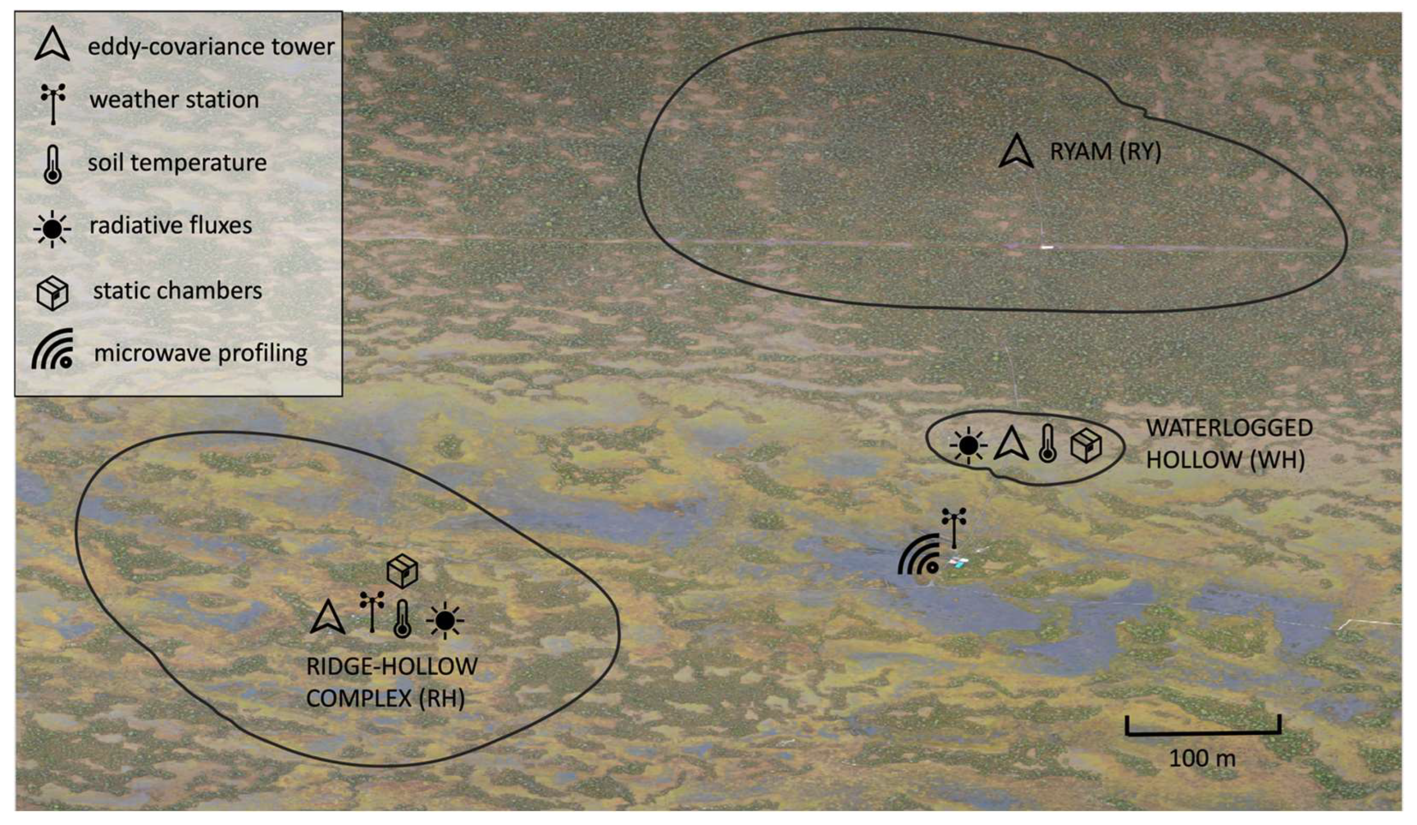
The summer field campaign was carried out in Mukhrino in the period 12–22 June 2022. Figure 1 presents an orthophoto plan showing the placement of observational platforms involved in this study. The used instruments and observed parameters are also summarized in

Table 1. Instruments and observational platforms used in the study.

Instrument/Sensor	Parameter	Accuracy	Platform	Location
Wind Monitor 05103 (R.M. Young Company, Traverse City, MI, USA)	Wind speed and direction at 2 and 10 m	Wind speed: ±0.3 m/s or 1% of reading Wind direction: ±3°	Stationary automatic weather station (AWS)	Ridge-Hollow
HC2A-S3 (Rotronic AG, Bassersdorf, Switzerland)	Air temperature and humidity at 2 m	±0.8% rh, ±0.1 K	Stationary AWS	Ridge-Hollow
CS105 PTB101b (Campbell Scientific, Inc., Logan, UT, USA)	Atmospheric pressure	±0.5 mb (at +20 °C)	Stationary AWS	Ridge-Hollow
CNR1 (Kipp & Zonen, Delft, Netherlands)	Short- and longwave up- and downwelling radiative fluxes	±10%	Stationary AWS	Ridge-Hollow
LI-7200 + LI-7700 (LI-COR, Inc., Lincoln, NE, USA) + uSonic-3 Cage MP (METEK GmbH, Elmshorn, Germany)	u,v,w—components of the wind vector, H2O, CO2, and CH4 concentrations at 20 Hz	Wind speed: 0.5%–1% at 5 m/s Direction: 1° at 5 m/s CO2 and CH4: within 1% H2O: within 2%	Eddy-covariance 7 m mast	Ridge-Hollow
Autonomous soil profile system, 9 probes × 8 sensors DS18B20	Soil temperature at 0, 2, 5, 10, 15, 20, 40, and 60 cm	±0.5 °C	Ridge-Hollow cross-section	Ridge-Hollow
Four closed chambers	CH4 emission			Waterlogged
WXT520 (Vaisala, Vantaa, Finland)	Wind speed and directions, air temperature and humidity at 2 m, atmospheric pressure	±0.5 hPa at 0 ... +30 °C ±0.3 °C ±3% at 10 m/s ±3% RH at 0 ... 90%	Temporary AWS	Hollow
MTP-5 (Attex, Dolgoprudny, Russia)	Air temperature profile up to 1000 m height with 50 m resolution	±1 °C		Hollow
iMet-XQ2 (InterMet Systems, Grand Rapids, MI, USA)	Air temperature and humidity	±0.3 °C ±5% RH	DJI Phantom 4 (DJI, Shenzhen, China)	Hollow
FLIR Tau 2 R Infrared Camera (Teledyne FLIR LLC, Wilsonville, OR, USA)	Surface brightness temperature	±2 °C or ±2%	DJI Mavic 2 (DJI, Shenzhen, China)	---
CNR4 (Kipp & Zonen, Delft, Netherlands)	Short- and longwave up- and downwelling radiative fluxes	±10%	Eddy-covariance 2 m mast	Waterlogged Hollow
LI-7200 + LI-7700 + Gill Windmaster (Gill Instruments Limited, Lymington, Hampshire, UK)	u,v,w –components of the wind vector, sonic temperature, H2O, CO2, and CH4 concentrations at 20 Hz	Wind speed: <1.5% Direction: 2° CO2 and CH4: within 1% H2O: within 2%	Eddy-covariance 2 m mast	Waterlogged Hollow
Davis soil station (Davis Instruments, Hayward, CA, USA)	Soil temperature at four levels (0, 5, 15, and 25 cm)	±0.5 °C	Eddy-covariance 2 m mast	Waterlogged Hollow
KT19 Infrared radiometer (HEITRONICS Infrarot Messtechnik GmbH, Wiesbaden, Germany)	Surface temperature	±0.5 °C	Eddy-covariance 2 m mast	Waterlogged Hollow
Two closed chambers	CH4 emission	-		Waterlogged Hollow
LI-7200 + uSonic-3 Cage MP	u,v,w—components of the wind vector, H2O, CO2 concentrations at 20 Hz	see above	Eddy-covariance 10 m mast	Ryam

. The orthophoto plan was created using images taken by the DJI Mavic 2 drone during the campaign.

We considered three contrasting sites where the eddy-covariance (EC) masts were located: the ridge-hollow complex (RH), the waterlogged hollow (WH), and the ryam (RY). These sites represent typical landscape types within the Mukhrino peatland.

It should be noted that ridges and ryam are covered with small trees and shrubs and are widely spread at raised ombotrophic peatlands [26]. In this respect, ridges differ from hummocks—another elevated form of a peatland microrelief. In comparison to hummocks, ridges have a relatively small size in cross-direction and a larger length along their axis. Also, the origin of ridges might differ from that of hummocks [27,28].

As can be seen in the orthophoto shown in Figure 1, the landscape within the RY and WH footprint areas is rather homogeneous, while a mixture of ridges and hollows is observed within the RH footprint. The size of the footprint areas varies due to the different heights of the EC masts: 10 m over RY, 7 m over RH, and 2 m over WH.

2.1. Meteorological Observations and Radiative Fluxes

The stationary automatic weather station (AWS) at the Mukhrino station is located at the RH site and provides wind speed and direction observations at 2 and 10 m, air temperature and humidity at 2 m, atmospheric pressure, as well as incoming and outgoing solar radiation. The data are stored every 30 s.

In addition to the local AWS, for the period of the campaign, one more AWS (WXT520, Vaisala, Vantaa, Finland) was installed at 2 m height, surrounded mainly by waterlogged hollows (Figure 1). It provided air temperature and humidity, atmospheric pressure, wind speed, and direction observations with a logging frequency of 1 min.

2.2. Vertical Profiling

The MTP-5 microwave profiler (Attex, Dolgoprudny, Russia) was installed at Mukhrino for the campaign period and provided vertical profiles of temperature every 5 min with a vertical resolution of 25 m in the lowest 200 m and 50 m in the layer 200–1000 m.

Vertical profiling up to 500 m height was also performed using the DJI Phantom 4 quadcopter (DJI, Shenzhen, China) with a meteorological payload, namely the iMet-XQ2 (InterMet Systems, Grand Rapids, MI, USA). iMet-XQ2 included air temperature, relative humidity, and atmospheric pressure sensors, as well as a GPS module. Data were logged at a 1 Hz sampling frequency. In addition, wind speed and direction during the flight were obtained from the Phantom 4 flight logs. Unfortunately, the description of the DJI algorithm for calculating wind speed and direction is publicly unavailable. Nevertheless, an earlier study [29] demonstrated a good agreement of wind speed and direction logged using Phantom 4 during a hover flight with the reference sonic anemometer observations. Previous studies describe the measurement and data processing techniques in more detail [29,30]. In Mukhrino, the UAV soundings were performed 2–4 times per day, apart from 17–19 June, when more frequent soundings were carried out in order to better resolve the diurnal cycle. In total, 44 sounding were performed during the campaign.

2.3. Eddy-Covariance Measurements and Surface Roughness Length Calculation

Three EC systems were operational during the campaign: two stationary ones installed at 7 m and 10 m heights over the ridge-and-hollow (RH) and ryam (RY) landscapes, respectively, and the temporary one at 2 m height over the waterlogged hollow (WH). All three systems were equipped with sonic anemometers and Licor-7200 H₂O and CO₂ gas analyzers, while only two, at RH and WH, included the Licor-7700 CH₄ gas analyzer. Vertical turbulent fluxes of momentum, heat, moisture, CO₂ and CH₄ were calculated using the Eddy-Pro software (version 7.0.9, LI-COR, Inc., Lincoln, NE, USA). For flux calculation, 30 min intervals were used for averaging. Footprint areas shown in Figure 1 were calculated using the Flux Footprint Prediction model [31].

In order to calculate the aerodynamic roughness length $z_{0m}$ we assume that for neutral stratification ($\left|z/L\right|<0.025$, where $L$ is the surface-layer Obukhov length) the log law is valid, namely

$$U_{\mathrm{z}}=\frac{u_{*}}{\mathsf{\kappa }}\mathit{ln}\frac{z}{z_{0\mathrm{m}}},$$

(1)

where $\mathsf{\kappa }=0.4$ is the von Karman constant; $u_{*}$ is friction velocity; and $U_{\mathrm{z}}$ is the wind speed at the observational height $z$. From (1) $z_{0m}$ can be found as

$$z_{0\mathrm{m}}=z{e}^{-\mathsf{\kappa }\frac{U_{\mathrm{z}}}{u_{*}}}.$$

(2)

It is important to note that (1) might not be applicable to some landscape types. In fact, it might be necessary to consider another length scale in (1), namely, the displacement height [32], especially over ryam and, perhaps, also over the ridge-hollow complex. Methods to estimate both the displacement height and $z_{0m}$ using the single-level sonic-anemometer data exist [33] and their application is left for future research. Nevertheless, our estimates of $z_{0m}$ using (1) serve to demonstrate at least qualitatively the variability of surface roughness.

2.4. Static Chamber Measurements

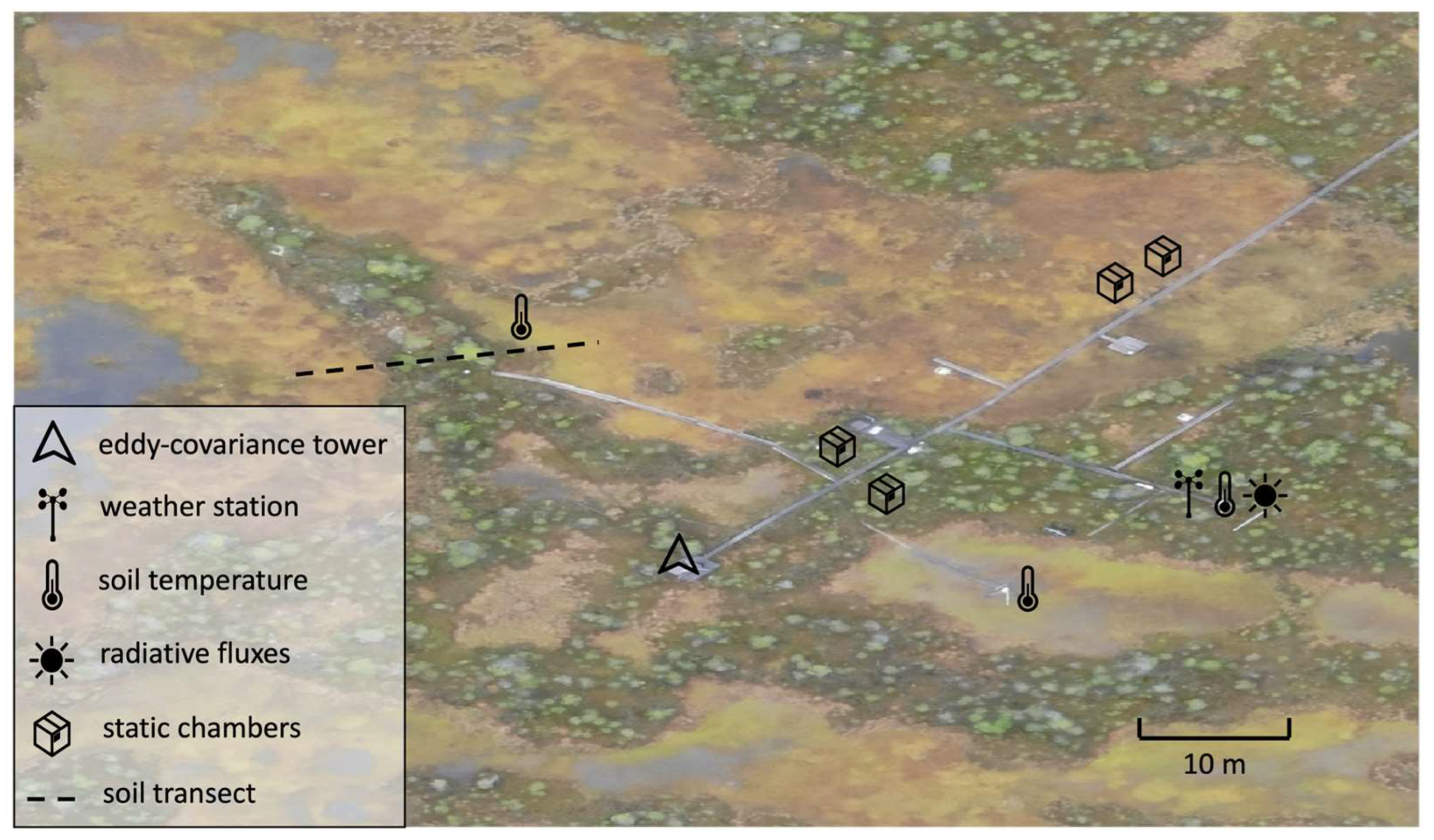
Static chamber measurements of methane emissions were organized at the RH (four chambers) and WH (two chambers) sites within the footprint of the eddy-covariance systems. In total, three locations were chosen, namely, (i) a ridge, (ii) a hollow at the RH site, and (iii) a waterlogged hollow at the WH site. Figure 2 shows a close-up orthophoto image of the RH site where the location of the four chambers is shown.

At each location, two Plexiglas chambers were installed on steel bases with 36 cm side lengths. Four chambers had 46.2 dm³ volume, and the other two had 64 dm³ volume. At each location, the temperature profile of the soil was measured using iButton sensors in addition to soil temperature measurements continuously carried out at Mukhrino.

Sampling was carried out five times per day for 10 days from 8:00 to 20:00 local time (at 08:00, 11:00, 14:00, 17:00, and 20:00). The chamber was set closed for 30 min at the hollow sites and 1 h at the ridge. Longer sampling time at the ridge is used due to smaller emissions than at hollows. Due to the detection limit of the gas chromatograph, a longer sampling time is needed in case of small emissions to determine fluxes with sufficient accuracy. In total, 730 samples were taken.

Samples were taken with a 60 mL syringe pumped under pressure into 15 and 20 mL hermetically sealed glass penicillin vials filled with saturated NaCl solution to avoid sample leakage and inhibition of biological activity in the vial. After collection, samples were stored and transported upside-down (i.e., the saline solution was at the bottom, and the gas sample at the top part of the vial) to further prevent sample leakage.

Methane concentration in samples was determined using the Kristall 5000.2 gas chromatograph (Chromatec, Yoshkar-Ola, Russia) with a flame ionization detector. A sample from each vial was injected into the chromatograph in two to four doses, depending on the available sample volume; the minimum volume of the injection was 4 mL. Methane fluxes were calculated following [34,35], assuming that methane concentration in a closed chamber either linearly increases in case of emission or exponentially decreases in case of consumption.

Each estimation of flux is based on four measurements of methane concentration. As flux error, the standard error of linear regression was taken for emission (positive flux values) and 95% confidence interval for consumption (negative flux values).

2.5. Soil Temperature Profiles

The soil temperature regime was studied using an autonomous soil profile system deployed at the RH site of the Mukhrino bog in July 2020. The complex included a datalogger, a data transmission system via a GSM network, an all-weather case for equipment, a solar panel, and a set of external soil temperature sensors. Each of the nine soil temperature probes consisted of eight sensors installed at the depths of 0, 2, 5, 5, 10, 15, 20, 40, and 60 cm below the surface. Temperature probes were placed along the hollow—ridge—hollow transect (Figure 2, dashed line), starting at the margin of the moss hollow to the north-east of the ridge, crossing the ridge about 10 m wide in a transverse direction and continuing in the south-western hollow with a shallow lake in the center. Two soil temperature probes were installed at the top of the ridge, three probes were at the slopes of the ridge, and four probes were with the hollows. The total length of the transect was 27 m. The maximal ridge height was about 40 cm above the hollow surface.

2.6. Infrared Surface Temperature Mapping

We used the DJI Mavic 2 Zoom quadcopter (DJI, Shenzhen, China) with the FLIR Tau 2 R thermal camera installed onboard for surface temperature mapping. The thermal camera had a 336 × 256 matrice size, an angle view of 35°, a focal length of 9 mm, and the spectral range of 7.5–13.5 microns. The camera was attached to the drone using a mounting kit and gimbal produced by DroneExpert company. The infrared imaging was carried out in scanning mode for parallel overlapping swaths; its results were further used to construct orthomosaics. We used DJI GS Pro software (v2.0.17, DJI, Shenzhen, China) to plan and run such scanning missions. In Mukhrino, we mapped infrared surface temperature for two separate areas covering ryam and ridge-hollow landscapes centered around the corresponding eddy-covariance towers (Figure 1). The size of each area was about 500 m × 500 m. The shooting height was set to 160 m, which ensured that such an area could be captured on a single battery charge in 10–12 min.

Primary data processing includes georeferencing of IR images based on quadcopter logs, their conversion from the format of radiometric JPEG to GeoTIFF, and correction of errors and artifacts of several types, including sharp temperature changes between successive images, and smoother temperature changes forced by the changes in heating and aspiration of the IR camera, which appear when a drone rotates or changes its tit angle. The data processing methodology, the listed errors, and methods for their correction are described in more detail in [36]. At the final stage of data processing, orthomosaics were constructed using the Agisoft Metashape software (v.2.1.0, Agisoft LLC, St. Petersburg, Russia) and exported in GeoTIFF format for further processing. The resolution of the resulting thermal orthomosaics was about 30 cm.

It is important to note that in the previous studies where the UAV thermal mapping was performed over peatlands [37,38], surface emissivity in the infrared was assumed to be equal to the constant value of either 0.97 or 0.98, and its spatial variability was neglected. We adopt the same strategy and, in the following, assume that spatial contrasts of brightness temperature are equal to those of surface temperature.

2.7. CH₄ Atmospheric Boundary Layer Budget Model

Here, we derive a method to estimate nocturnal emissions of CH₄ using the observed increase in the CH₄ mixing ratio $\mathsf{\chi }$ during the night and the observed height of a stably stratified ABL.

Assuming that the nocturnal mixing ratio rise is due to the surface flux only, we can neglect horizontal advection so that the conservation equation for $\mathsf{\chi }$ can be written as follows [39] (Equation (1.13))

$$\overline{{\mathsf{\rho }}_{\mathrm{d}}}\frac{\partial \mathsf{\chi }}{\partial t}=-\frac{\partial \overline{{\mathsf{\rho }}_{\mathrm{d}}}\overline{w^{\prime }{\mathsf{\chi }}^{\prime }}}{\partial z},$$

(3)

where $\overline{{\mathsf{\rho }}_{\mathrm{d}}}$ is the molar density [mol m⁻³] of dry air. Let us assume that (i) during the night, the ABL height $h$ is time-invariant, (ii) $\overline{{\mathsf{\rho }}_{\mathrm{d}}}$ is constant throughout a shallow ABL, and (iii) the entrainment flux of $\mathsf{\chi }$ at the ABL top is negligible. Then, integrating (3) over z from z = 0 to z = h, one obtains

$$\overline{{\mathsf{\rho }}_{\mathrm{d}}}\frac{\partial }{\partial t}{\int }_0^h\mathsf{\chi }\mathrm{d}z=\overline{{\mathsf{\rho }}_{\mathrm{d}}}{\left(\overline{w^{\prime }{\mathsf{\chi }}^{\prime }}\right)}_{\mathrm{s}},$$

(4)

where the subscript “s” denotes the flux at the surface. Let us assume that in a stable ABL $\mathsf{\chi }$ is changing linearly with height from its surface value ${\mathsf{\chi }}_{\mathrm{s}}$ to the time-independent background value ${\mathsf{\chi }}_{\mathrm{h}}$ at z = h, namely

$$\mathsf{\chi }\left(z\right)=\frac{{\mathsf{\chi }}_{\mathrm{s}}-{\mathsf{\chi }}_{\mathrm{h}}}{h}\left(h-z\right)$$

(5)

After we use (5) in (4), we obtain

$$\overline{{\mathsf{\rho }}_{\mathrm{d}}}{\left(\overline{w^{\prime }{\mathsf{\chi }}^{\prime }}\right)}_{\mathrm{s}}=\frac{h\overline{{\mathsf{\rho }}_{\mathrm{d}}}}{2}\frac{\partial {\mathsf{\chi }}_{\mathrm{s}}}{\partial \mathrm{t}}.$$

(6)

We keep $\overline{{\mathsf{\rho }}_{\mathrm{d}}}$ in (6) so that the surface methane flux $F_{\mathrm{s}}=\overline{{\mathsf{\rho }}_{\mathrm{d}}}{\left(\overline{w^{\prime }{\mathsf{\chi }}^{\prime }}\right)}_{\mathrm{s}}$ has the same units [μmol s⁻¹m⁻²] as the output of the EddyPro software used for processing the eddy-covariance data. From (6), it is obvious that the surface flux of methane can be found using the observed increase in the near-surface CH₄ mixing ratio and the ABL height h. It should be noted that a similar boundary-layer budget approach has already been used previously to estimate methane fluxes [40] also during the night [41,42].

There are, however, several challenges associated with the practical use of (6). First of all, one has to measure or estimate the ABL height. When no soundings are available, the ABL height can be estimated using surface observations and one of the parameterizations proposed earlier [43,44]. When soundings are available, several criteria can be used to identify the stable ABL height, but as shown further, this is not straightforward for very strong stability. Second, it is a question to which area one can attribute the surface methane flux estimated using (6). The latter question requires separate research and is out of the scope of this study.

3. Results

3.1. Basic Meteorology and Radiative Budget

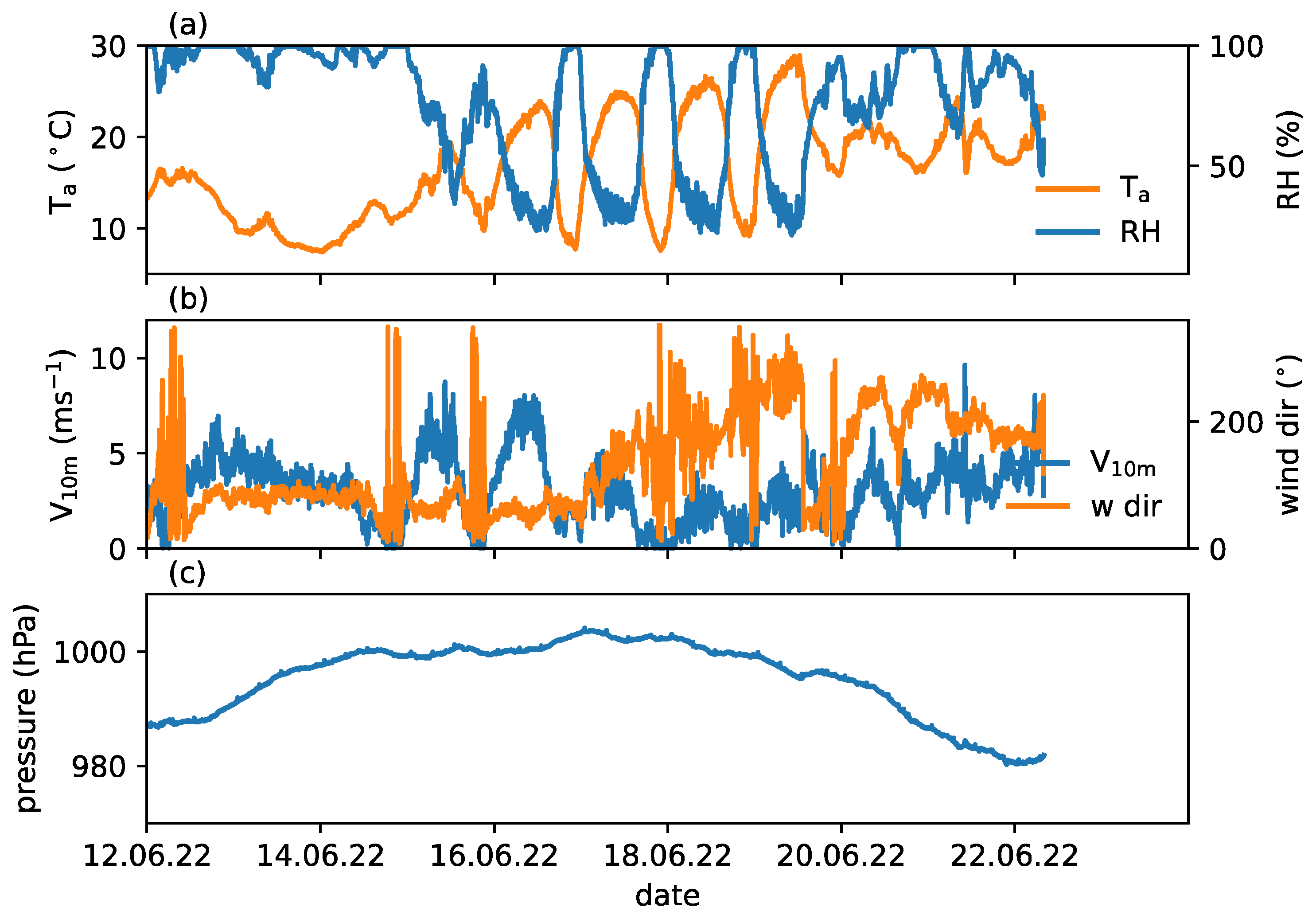
Figure 3 presents the time series of the main meteorological variables. Three periods can be clearly identified. The first period, from 12 to 16 June, was characterized by rainy weather with steady wind and a weak diurnal cycle. Air temperature during this period did not rise higher than 20 °C. The second period, lasting from 16 to 20 June, was a period of high pressure, clear-sky conditions, and a strong diurnal air temperature and wind speed cycle. The maximum daily temperature steadily increased during this period and reached almost 30 °C on 19 June. Nocturnal air temperature dropped below 10 °C. With low wind speed, this points to developing a strongly stable boundary layer during the night. Relative humidity reached 100% during such nights, but almost no fog was observed. After 20 June, atmospheric pressure fell, and stronger wind and more cloudy conditions were observed.

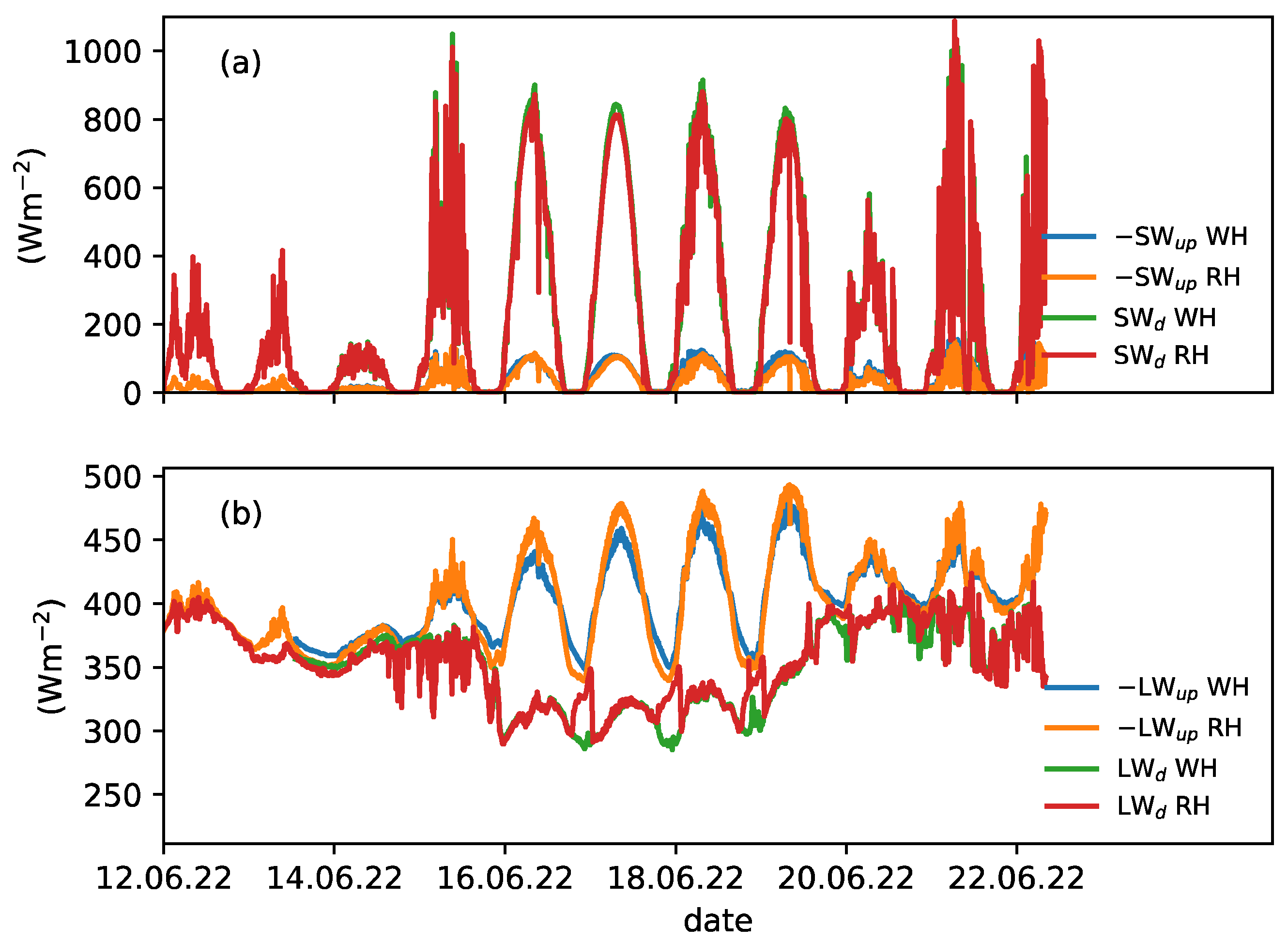
The three periods are also clearly visible in the radiative fluxes, as shown in Figure 4. The first period was characterized by relatively small values of the downwelling shortwave radiative flux reduced due to cloudiness. For the same reason, the downwelling longwave radiative flux was increased, which resulted in small values of the net longwave flux. During the second period, the downwelling shortwave flux was not affected by clouds, and the downwelling longwave flux was reduced. This period was characterized by large negative values of net longwave flux, especially during the daytime. In the third period, the effect of clouds again became more pronounced, not only in the downwelling shortwave flux but also in the increased values of the downwelling longwave flux.

In general, radiative fluxes at the two observational sites agree well. Nevertheless, there are several important differences. First, there was a clear difference in the upwelling longwave flux, which points to a difference in surface temperature. This aspect is discussed in more detail in the next subsection. Second, a sudden increase in the downwelling LW flux was observed during several nights at the RH site. Such an increase was missing at the WH site. The reason might be the dew, which could have condensed on the surface of the sensor during clear-sky nocturnal cooling. This is also supported by the 100% values of relative humidity measured at the RH site during the clear-sky nights.

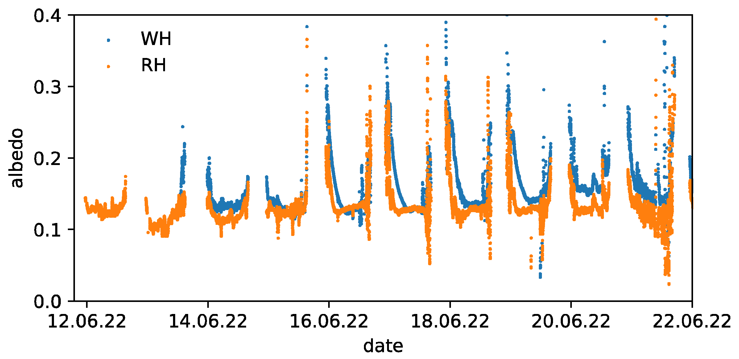
Finally, it is important to consider the albedo differences between the two sites. Figure 5 shows the broadband shortwave albedo calculated using the measured upward and downward shortwave fluxes. During the daytime, the average albedo values were similar at both sites and were about 0.12–0.15, which is in the range of values typically observed over peatlands [45]. In the latter study, the median albedo of peatlands for July amounted to 0.12, ranging from 0.1 to 0.16. Albedo at the WH site showed increased dependency on the sun elevation angle in the morning hours during the clear-sky period. This resulted in about a 20 Wm-2 difference in the reflected solar radiative flux. The effect of a high water table level can explain the albedo increase at a low sun angle. Open water patches were numerous at the WH site and might have increased reflectivity, while at the RH site, the effect of open water patches was obstructed by ridges and shrubs. Such a dependency of albedo on the sun-elevation angle at WH is clearly less pronounced during cloudy conditions.

3.2. Surface Temperature

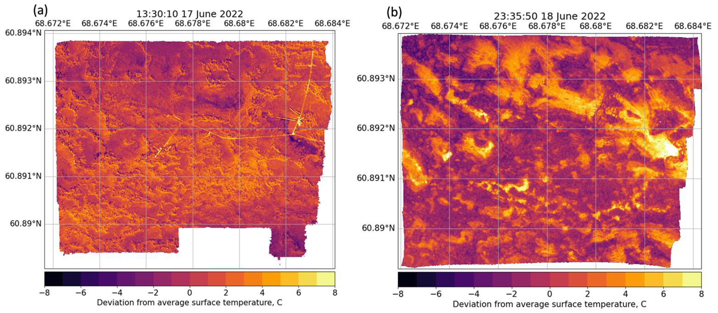
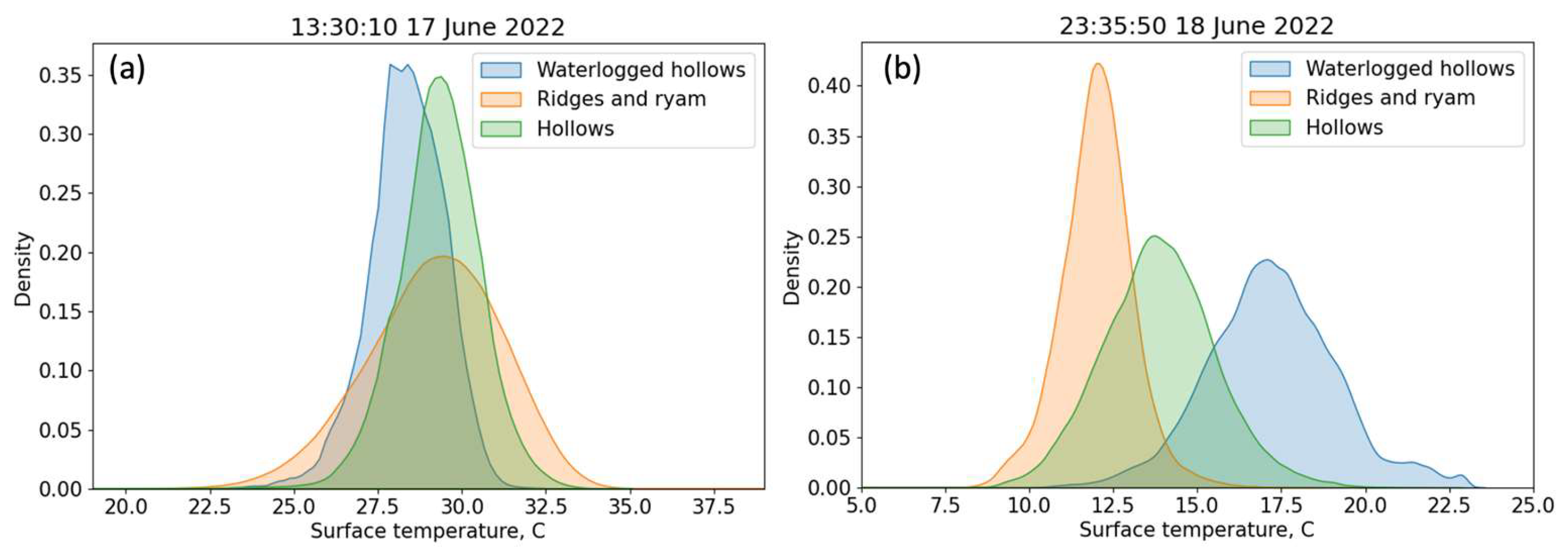
The results of the IR mapping reveal striking contrasts of surface temperature across the peatland microlandscapes. Figure 6 presents the two orthomosaics based on the UAV IR mapping obtained during the day- and night-time conditions over the ridge-hollow complex, waterlogged hollows, and shallow lakes. The color shading corresponds to the deviation of surface temperature from its spatially averaged values. The surface temperature’s probability density functions (PDF) were further obtained for different landscape types based on the IR-mapping results. The PDFs in Figure 7 correspond to the same time periods as orthomosaics in Figure 6. During the day, the highest surface temperature was observed at the southern slopes of ridges and within some relatively dry hollows. Wet hollows where the water-table level reached the surface and shallow lakes remained colder during the day. The northern slopes of ridges and their shadowed parts also remained colder, which explains why the daytime PDF of the surface temperature is the widest for ridges. During the day, the contrast in surface temperature reached 10 °C between the warmest and coldest parts of the peatland, i.e., between the southern slopes of ridges and cold lakes.

At night, the spatial distribution of surface temperature was somewhat reversed. Ridges and ryam became the coldest elements of the landscape, while lakes and wet hollows remained warm. At night, the temperature difference between the warmest and coldest elements of the landscape exceeded 10 °C, and temperature differences between micro-landscapes became stronger—the three PDFs in Figure 7b are well separated.

The most obvious reason for the observed temperature contrasts is the elevation of microrelief relative to the water-table level. The heat capacity of drier ridges is much smaller than that of water. Hence, the surface temperature of ridges quickly follows changes in radiative balance, while the inertia of waterlogged hollows and lakes is much larger.

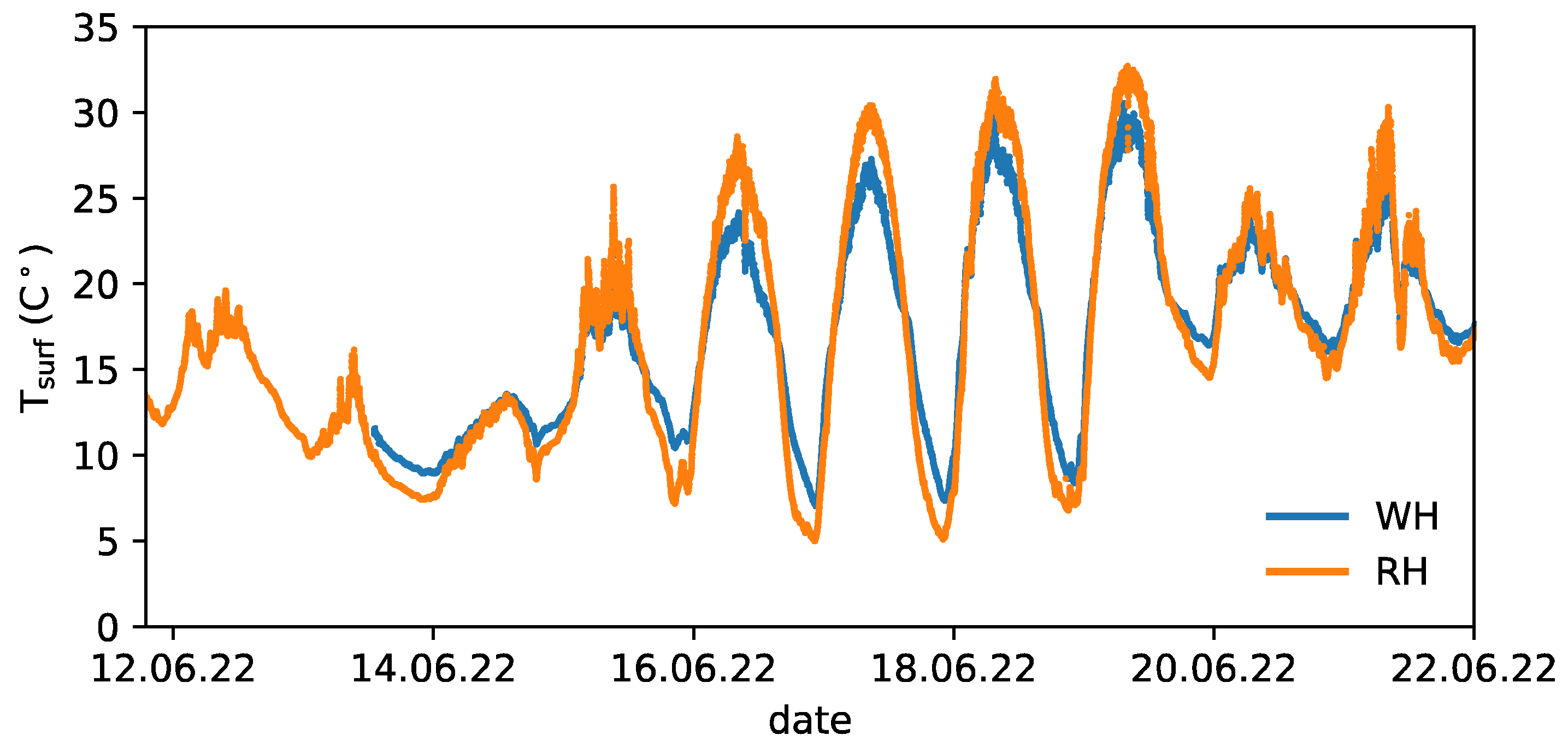
The surface temperature time series derived from the upwelling longwave radiative flux over the ridge and the waterlogged hollow reveal similar peculiarity (Figure 8). The ridge surface temperature exceeded that of the waterlogged hollow during the day by an amount of up to 3–4 °C but was lower by about 3 °C during the night. As expected, the contrast in surface temperature was largest during the clear-sky period.

3.3. Soil Temperature

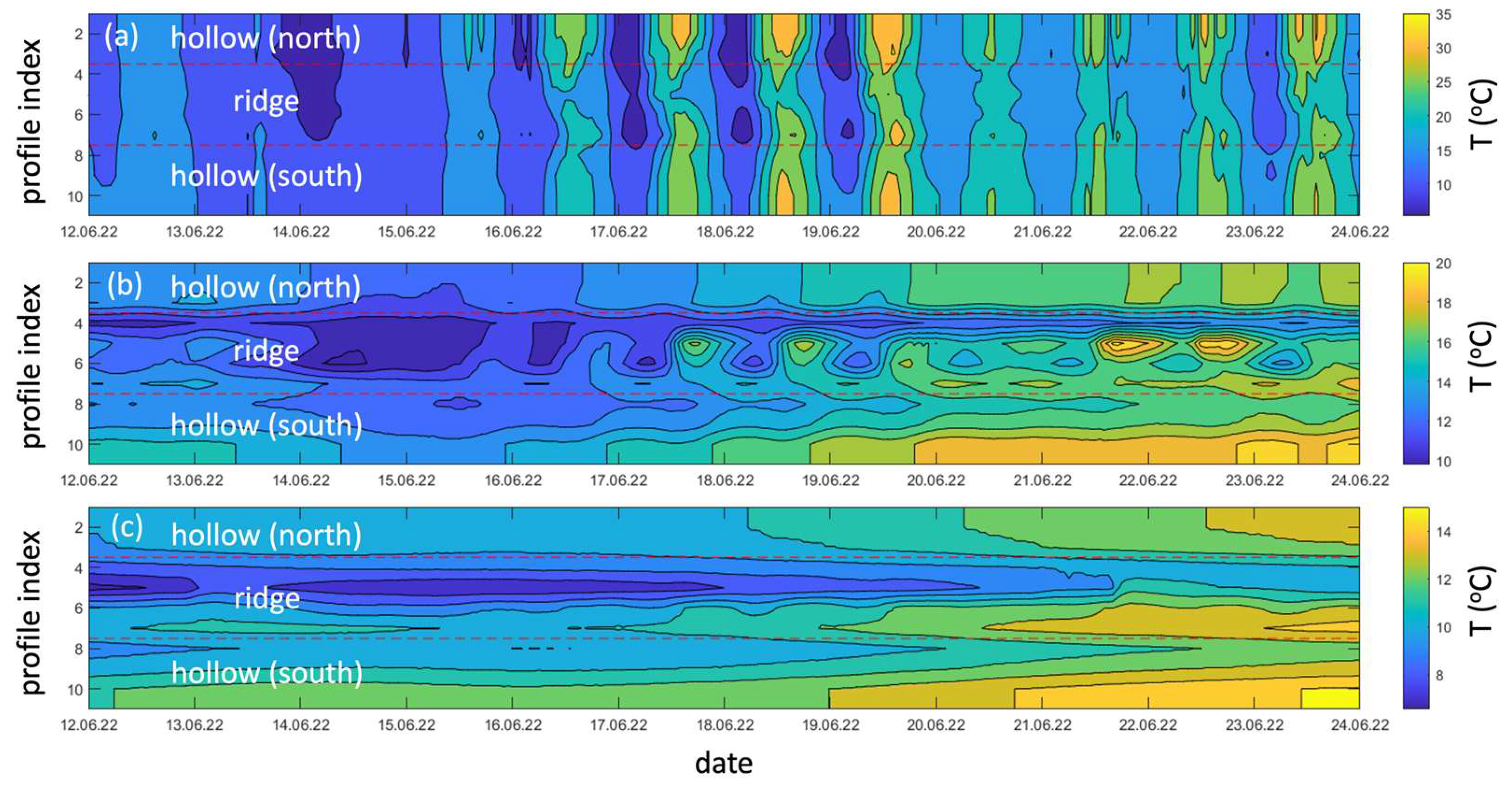
The soil temperature variations along the hollow-ridge-hollow transect are shown in Figure 9. The horizontal axis represents time, and the vertical axis represents the number of probes along the transect. The dotted red lines show the ridge boundary. The northern hollow is in the upper part of each plot, while the southern hollow is in the lower part. Color shading indicates temperature.

Figure 9a shows the spatial and temporal variability of surface temperature. On cool days (12–15 June), the surface temperature on the ridge and hollow was practically the same (+10 ÷ +18 °C), except for the night of 14 June, when the temperature on the ridge and northern hollow dropped to +8 °C. With the onset of clear days (16–20 June), the diurnal cycle of surface temperature became especially strong, and temperature contrasts between elevated and lowered microrelief elements became noticeable. During daytime hours, the northern hollow is heated up to +32.4 ÷ +33.5 °C, which is slightly higher than the surface temperature on the southern hollow (+29.3 ÷ +31.2 °C) and higher than on the ridge (+29.5 ÷ +32.8 °C). However, even at noon on the ridge, there are areas with lower surface temperatures (+18.8 ÷ +25.1 °C), probably in the shade of trees. As a rule, the hollow is warmer than the ridge at night. The surface temperature of the southern hollow (+12.5 ÷ +15.3 °C) is higher than that of the northern one (+6.2 ÷ +9.3 °C). As in the daytime, during the night hours, the surface temperature of the ridge is heterogeneous and varies from +7.3 to +12.1 °C; however, it is lower than the surface temperature of the northern hollow.

At a depth of 20 cm from the surface (Figure 9b), the diurnal temperature variation in hollows was largely smoothed out; its amplitude decreased to 1 °C, while at the ridge, the amplitude of the diurnal variation was 5–7 °C. In the daytime, the 20 cm soil temperature at the ridge became higher than at the hollow. At night, the ridge was colder than the hollow at the 20 cm depth.

Starting from the depth of 40 cm and below, the diurnal temperature variations became very small, and differences in soil temperature of different hollows became visible (Figure 9c). The southern hollow was warmer than the northern one by 1.5–2 °C. Within the ridge, differences in the temperature of the northern and southern slopes are revealed. The northern slope of the ridge is colder than the southern slope.

3.4. Turbulent Fluxes of Sensible and Latent Heat

Before discussing spatial contrasts of sensible and latent heat fluxes, it is important to consider differences in surface roughness over various landscape types.

Table 2. Roughness length for momentum over three different landscape types.

Landscape Type	$\mathbf{Roughness}\mathbf{Length}{\mathit{z}}_{0\mathbf{m}}$ [m]
Waterlogged hollow (WH)	0.08
Ridge-hollow complex (RH)	0.17
Ryam (RY)	0.50

shows roughness lengths over three different landscape types obtained using (2) with the observed values of $u_{*}$ and $U_{\mathrm{z}}$, and averaged throughout the campaign. The largest value of $z_{0\mathrm{m}}$ amounting to 0.50 m is found for the RY site, which is not surprising as ryam is covered with trees and shrubs. The smallest value of $z_{0\mathrm{m}}$ amounting to 0.08 m is obtained for WH. This is also expected, as just a few trees are found at the WH site within the footprint. The RH site is characterized by $z_{0\mathrm{m}}$ values of 0.17 m being smaller than those over RY and larger than those over WH, which is also expected as RH represents a mixture of hollows and ridges covered with trees and shrubs.

Alekseychik et al. [20] reported the value of $z_{0\mathrm{m}}=0.12$ m using eddy-covariance measurements over RH in Mukhrino averaged over the period May-August. Their value is slightly lower than 0.17 m observed during our campaign, which might be due to the fact that $z_{0\mathrm{m}}$ depends on the leaf area index and reaches maximum values in July–August over boreal peatlands [46,47]. It is important to note that in both latter studies, the reported values of $z_{0\mathrm{m}}$ were close to our estimates over WH, but lower than over RH and RY. Namely, Shimoyama et al. [46] measured $z_{0\mathrm{m}}$ in the range 0.02–0.07 m over a hummock-hollow landscape of a West-Siberian peatland. Alekseychik et al. [47] obtained the values of $z_{0\mathrm{m}}$ below 0.07 m over a fen and a hummock-hollow landscape in Finland. It is important to note that the vegetation in both landscapes was dominated by sedge and not by shrubs and trees like in the case of RH and RY in Mukhrino, which explains higher $z_{0\mathrm{m}}$ values obtained in our study. The $z_{0\mathrm{m}}$ values over RY are in the range typically observed over forests which is 0.3–1 m [46] (their Table 1).

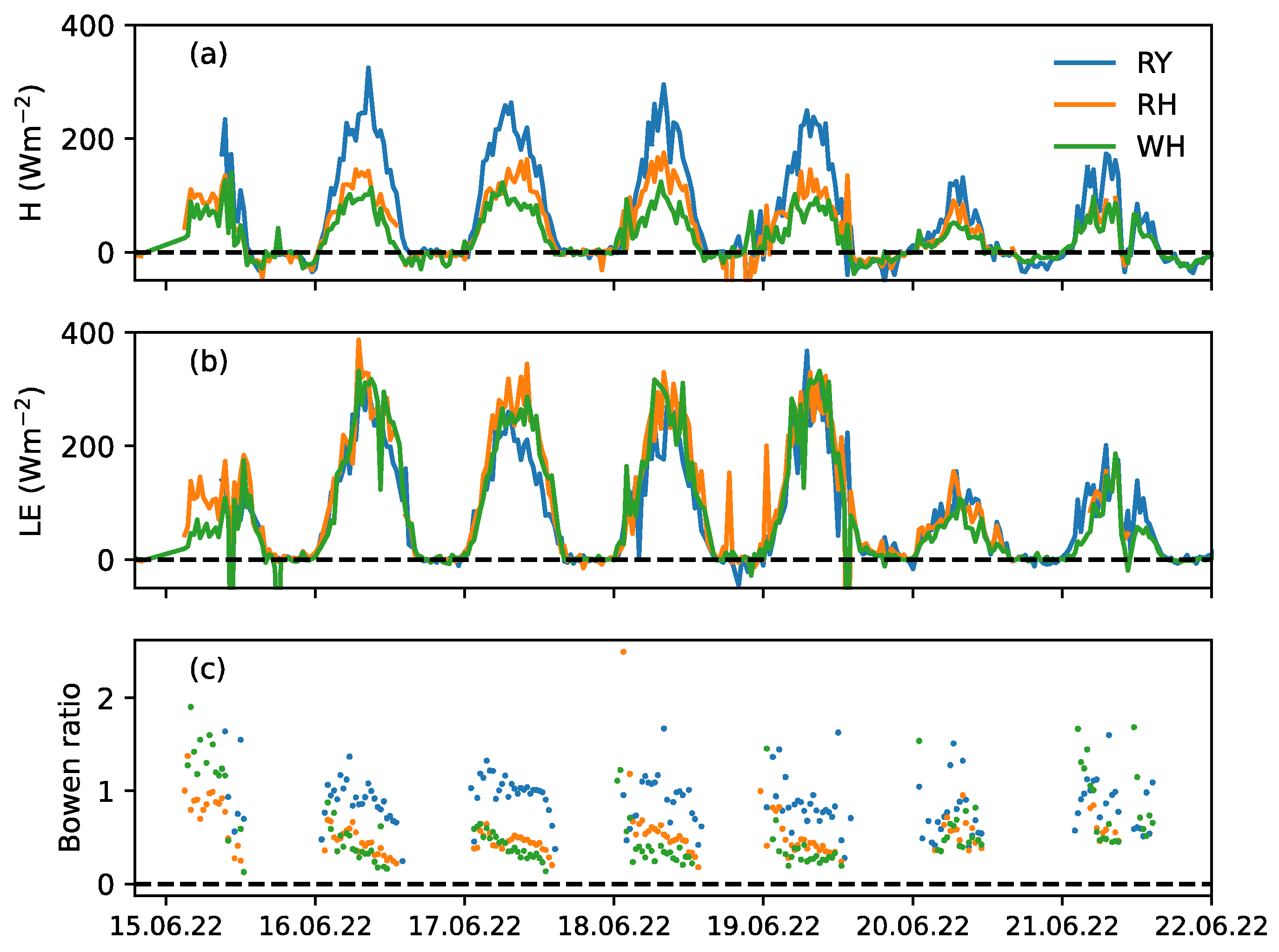
The daytime spatial distribution of surface temperature (Figure 6a), as well as the variation of $z_{0\mathrm{m}}$ explains the variation of the observed sensible heat flux $H$ across the landscapes, as shown in Figure 10a. Clearly, the largest values of $H$ exceeding 250 Wm⁻² were observed during daytime at the RY site. The smallest values of $H$ amounting to 100 Wm⁻² were found at the WH site. The sensible heat flux values at the RH site were between those at WH and RY and amounted to about 150 Wm⁻² during the daytime.

As far as the temporal variation of $H$ is concerned, the largest values of $H$ were observed during the clear-sky period from 16 to 19 June. During this period, also the largest values of latent heat flux $LE$ exceeding 300 Wm⁻² were observed (Figure 10b). Also, one can see much less variation of $LE$ across landscapes. Latent heat flux at the RY site was only slightly smaller than that over WH and RH, although the surface of ryam was substantially elevated over the water-table level. We hypothesize that larger roughness and increased evapotranspiration (the latter was not measured during the campaign) helped to maintain large values of $LE$ over ryam.

The Bowen ratio $\beta =H/LE$ also demonstrates a clear spatial variation across landscapes (Figure 10c). During the clear-sky period, the largest values of up to 1 were observed over ryam, being closer to those over boreal forests and exceeding the value of 0.5 typically found for peatlands [45]. The smallest values of $\beta$ were observed over the WH site, while $\beta$ over RH was close to 0.5. The Bowen ratio also showed a pronounced temporal variability. Over WH and RH, $\beta$ clearly increased during colder cloudy periods due to decreased latent heat flux.

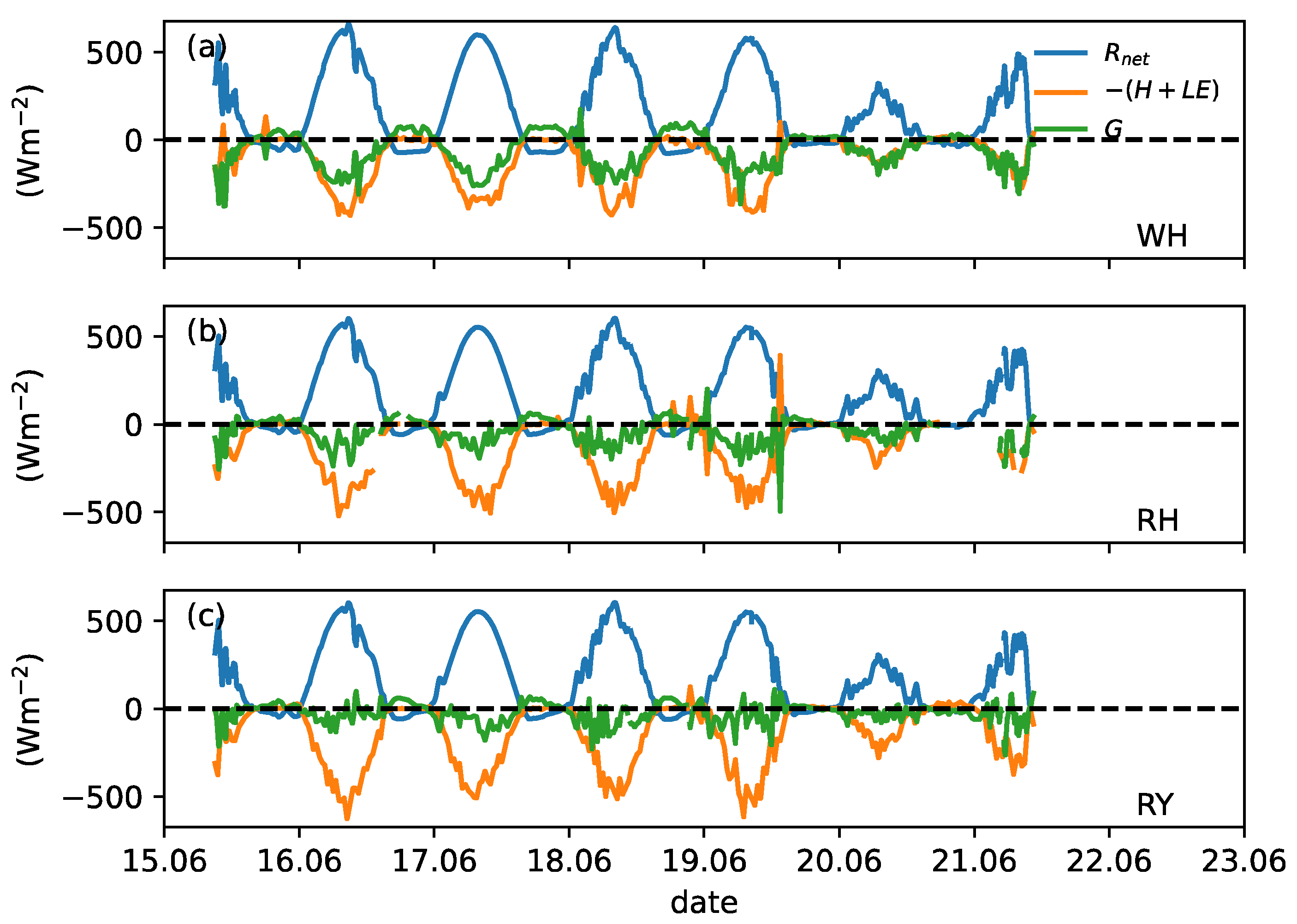
Finally, it is important to consider the terms of the heat balance equation [48] (Equation (5.1)): the net longwave radiative flux $R_{net}$, turbulent fluxes of sensible and latent heat, as well as the residual term $G$ which can be interpreted as the soil heat flux (Figure 11). Here, we did not explicitly calculate the soil heat flux using the soil temperature profiles—this remains a subject of future research. Figure 11c shows that over ryam, nearly the entire amount of the incoming net radiation was returned to the atmosphere via turbulent fluxes. The value of the soil heat flux there was small. The soil heat flux was much larger at WH and RH. This shows that, indeed, hollows accumulated large amounts of heat during clear-sky periods, and this accumulated heat helped hollows stay warm during the night.

3.5. CH₄ Emissions

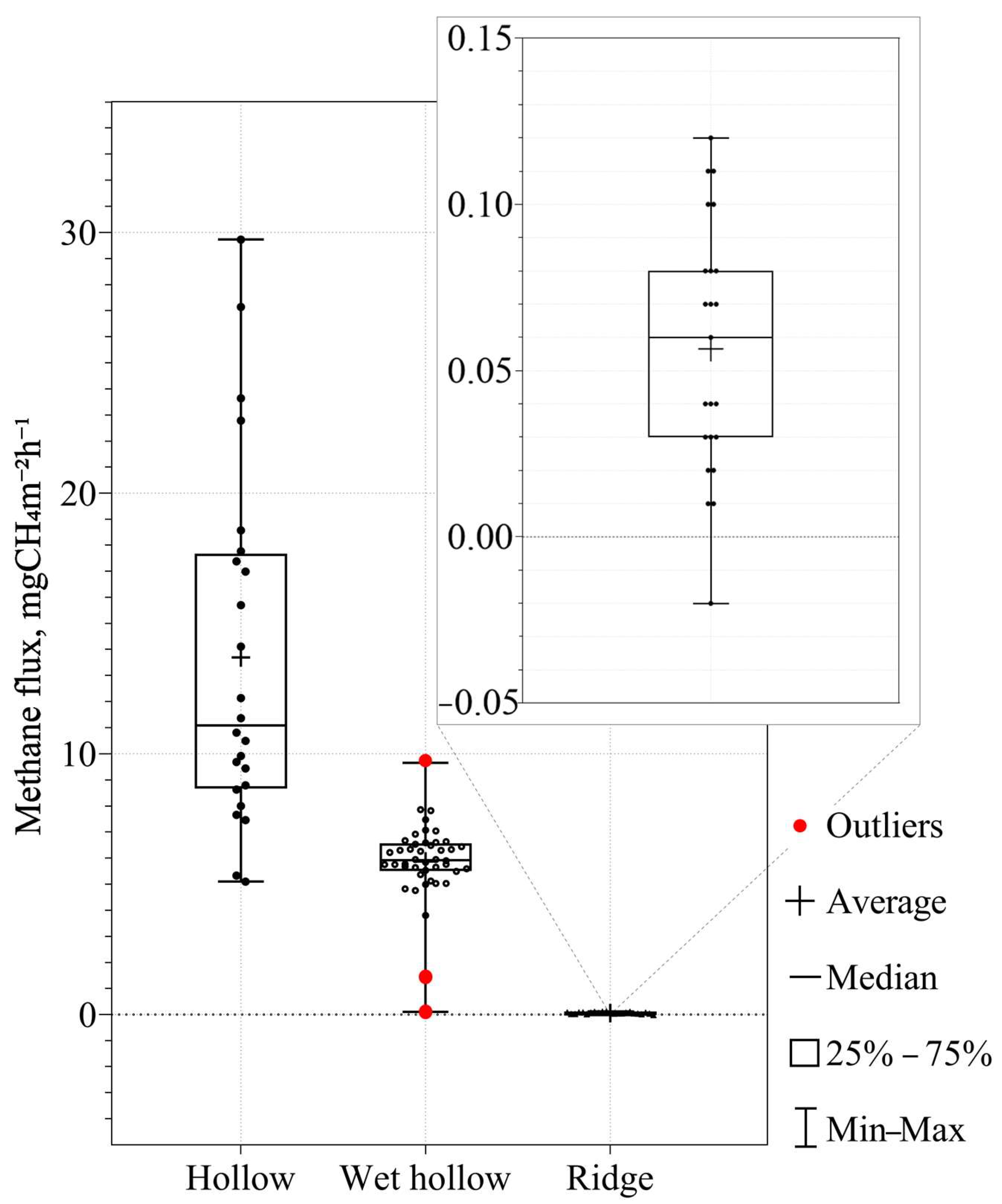
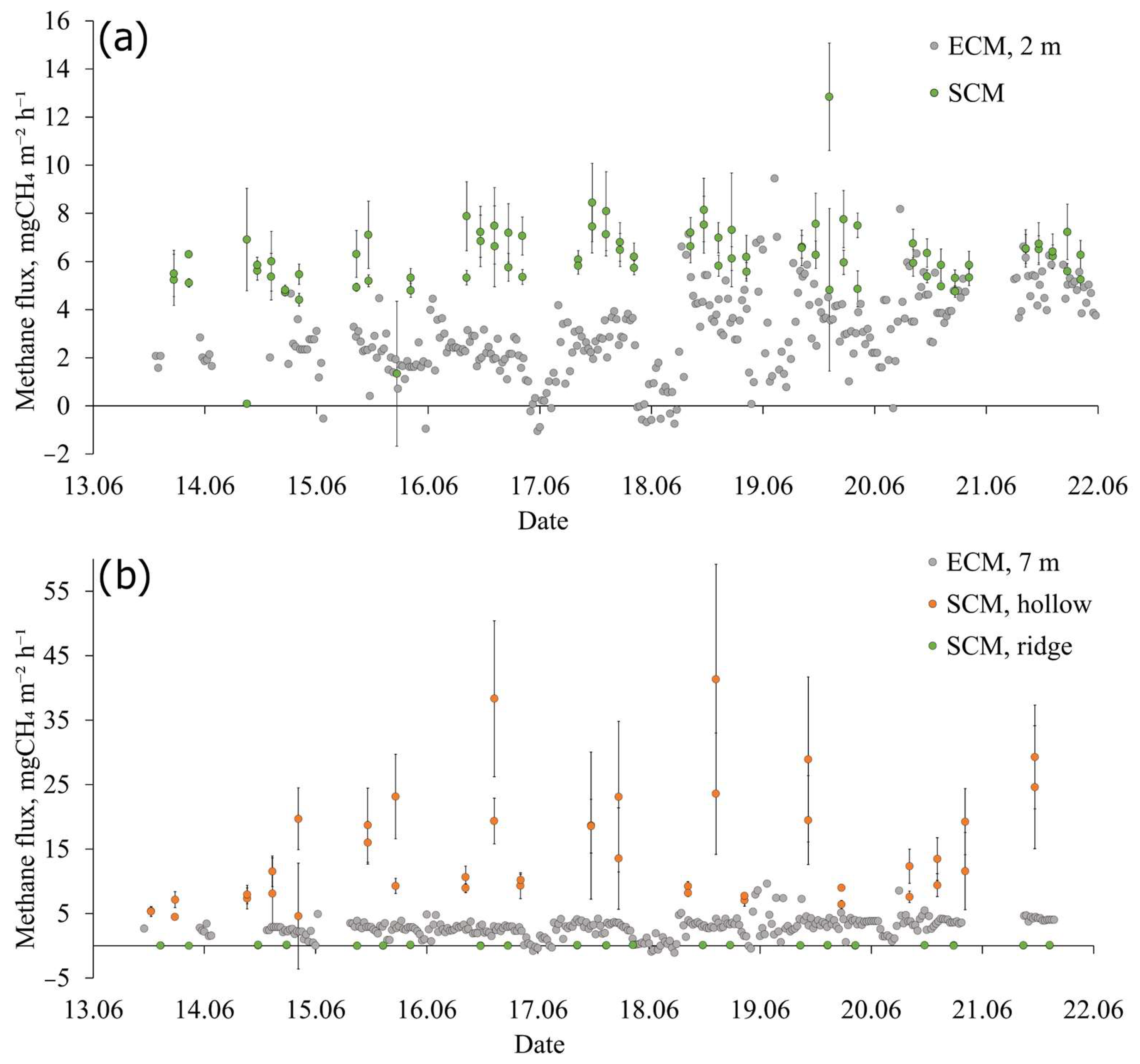
Methane fluxes from different observational sites measured using the static chamber method are shown in Figure 12. Methane flux demonstrates strong variability across landscapes. Namely, the largest emissions are found over hollows, while CH₄ flux over the ridge was close to zero. The position of the water table level can explain this. The latter was far below the ridge surface. The typical elevation of the ridge over the water-table level was about 40 cm. In contrast, the water-table level varied from 10.5 to 4 cm below the hollow surface at RH and from 3 cm below the surface to 1 cm above the surface at WH, thereby preventing methane oxidation and methanotrophic activity. These results support previous conclusions based on observations at Siberian peatlands and at Mukhrino [23,24]. It should be noted that the median values of CH₄ flux from the hollow and the waterlogged hollow (6 and 11 mgCH4 m⁻² h⁻¹, respectively) fall well within the range of methane emissions from hollows reported for Mukhrino earlier [24], although slightly exceed the median values. Also, according to static chamber observations in Mukhrino in August-September 2020 [25], methane emissions in hollows amounted to 3.7 ÷ 5.0 mgCH4 m⁻2 h⁻¹, lower than during our campaign.

It might be puzzling why methane emissions from the hollow at RH were larger than those from the hollow at WH, although the water table level at the latter site was higher. Additional observations are needed in order to draw any conclusions. We can only hypothesize that the available organic matter could have been already largely decomposed at the WH site, so methanogens had less substrate. In addition, at high water table levels, CH₄ emissions might be decreased due to the high dissolved O₂ content in water and also due to the influence of the water layer on methane transport to the surface [49].

Figure 13a,b compares CH₄ fluxes obtained using the static-chamber and eddy-covariance methods (SCM and ECM, respectively). Over the more homogeneous WH site, the two methods result in flux values that are rather close to each other (Figure 13a), although on some days, the values obtained using SCM exceed those of ECM by about a factor of two. This might be because ridges and parts of the neighboring ryam occupied some fraction of the footprint area at WH. This might have reduced the overall CH₄ flux obtained using ECM.

A much larger discrepancy between the results of the two methods is found over the RH site (Figure 13b). Namely, the methane flux obtained using SCM over the hollow is several times larger than the ECM methane flux. One of the reasons is clearly the heterogeneity of landscape within the footprint of the EC tower. A large fraction (roughly 40%–50%) of the footprint area is covered by ridges (Figure 1) and shallow lakes, reducing the overall CH₄ flux measured by ECM.

Finally, Figure 13a shows that the ECM fluxes and, to some extent, the SCM fluxes demonstrate a diurnal cycle with elevated fluxes during the day and reduced fluxes at night. Unfortunately, static-chamber observations were not carried out during the night but included the morning and evening hours. The observed diurnal cycle might manifest a dependency of methane flux on environmental factors such as soil temperature and wind speed. However, the results of ECM during weak winds and strongly stable conditions during some nights need to be considered with caution, as the uncertainty of the standard EC approach increases during weak and intermittent turbulence conditions.

3.6. Nocturnal CH₄ Accumulation in the ABL

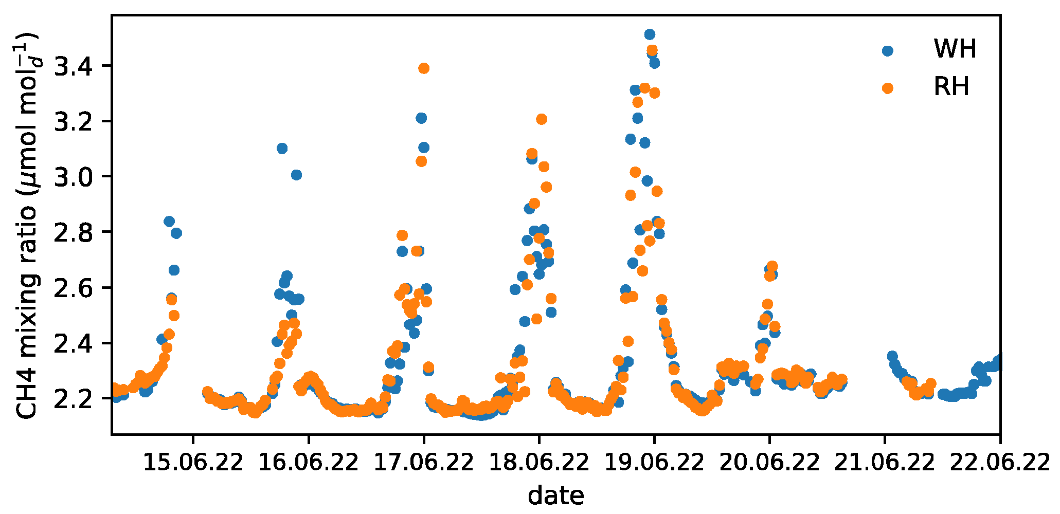
The time series of the CH₄ mixing ratio ${\mathsf{\chi }}_{\mathrm{s}}$ shown in Figure 14 shows clear nocturnal peaks up to 3.4 μmol/mol_d, while during the daytime, the values go back to about 2.1–2.2 μmol/mol_d. Such a diurnal cycle can be clearly explained using diurnal dynamics of the ABL stratification and height. During the night, a shallow, stably stratified ABL forms. Turbulent mixing weakens, and emitted methane accumulates near the surface. During the day, a well-mixed unstable ABL develops and effectively mixes the near-surface concentration over the thick ABL. Moreover, as the convective ABL grows, it entrains air from aloft with background concentrations of CH₄.

According to the eddy-covariance method, CH₄ flux reduces to small, almost near-zero values during the nights of accumulation (Figure 13a,b), especially during weak-wind conditions and increased stability. However, nocturnal accumulation of CH₄ near the surface clearly points to nonzero emissions. In order to resolve such a contradiction, first of all, a careful analysis of nocturnal turbulence data is needed to reduce the uncertainty of the eddy-covariance technique. This forms a separate research topic that is beyond this study’s scope. Nevertheless, already here, we would like to apply the boundary-layer budget method (Section 2.7) to show that it can be used to provide one more independent estimate of nocturnal emissions.

As shown in Equation (6), in order to calculate the surface methane flux, one needs to estimate the height of the nocturnal stably stratified ABL. To that aim, we use the UAV vertical soundings.

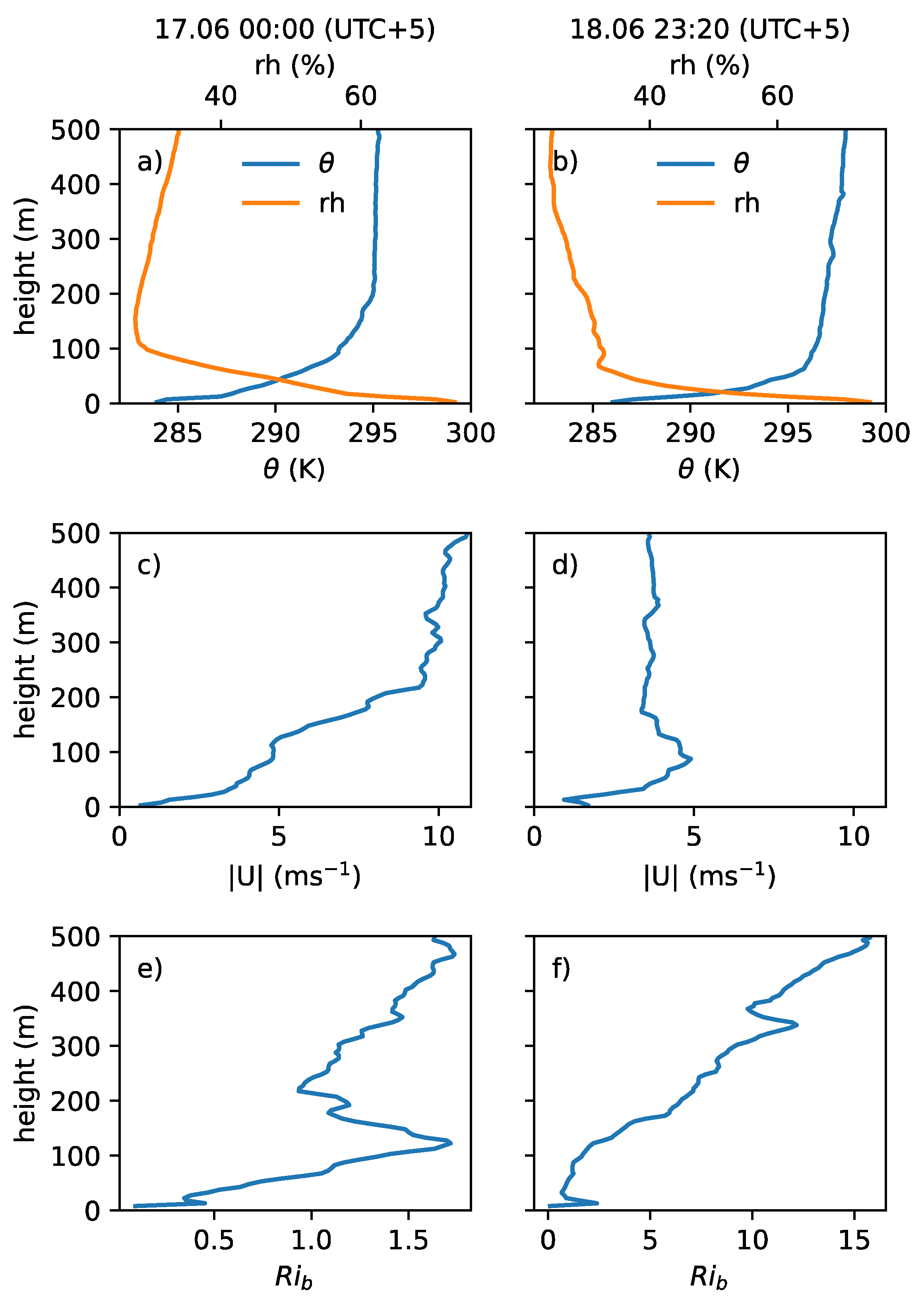
Figure 15 shows the vertical profiles of potential temperature, relative humidity, wind speed, and bulk Richardson number based on the UAV soundings carried out during night-time on 16–17 and 18 June. The bulk Richardson number is defined as

$$\mathrm{R}{\mathrm{i}}_{\mathrm{b}}=\frac{g/{\mathsf{\theta }}_0\left(\mathsf{\theta }\left(z\right)-{\mathsf{\theta }}_0\right)z}{u{\left(z\right)}^2+v{\left(z\right)}^2},$$

(7)

and its critical value is often used to determine the ABL height from the vertical profiles of temperature and horizontal wind components [50,51].

On both nights, a shallow, stably stratified ABL and strong temperature inversion are clearly identified (Figure 15a,b). The potential temperature increase in the layer 0–100 m amounted to about 10 K. Above this stable layer is a residual layer with a near-zero or very small potential temperature lapse rate. Obviously, the stable layer was produced by nocturnal cooling. The height of this layer can be identified from the potential temperature and relative humidity profiles, and it was about 100–125 m on 16–17 June and about 60–80 m on 18 June. The lower wind speed can explain the lower height on 18 June (Figure 15c,d). The latter amounted to about 10 ms⁻¹ in the residual layer on 16–17 June and 4 ms⁻¹ on 18 June.

Vertical profiles of $\mathrm{R}{\mathrm{i}}_{\mathrm{b}}$ show a rapid increase in its value with height, especially on 18 June (Figure 15e,f). The critical values of $\mathrm{R}{\mathrm{i}}_{\mathrm{b}}$, which were proposed earlier for determining a stable ABL height lie between 0.24 [51] and 0.6 for $h/L\approx 10$ corresponding to moderate stability [50], where $L$ is the surface-layer Obukhov length. Obviously, on both nights, $\mathrm{R}{\mathrm{i}}_{\mathrm{b}}$ exceeded the proposed critical values already in the first 20–30 m above the ground. Based on this, we can hypothesize that stratification on both nights was so strong that the cooling layer was perhaps not fully turbulent. It is important to note that Richardson et al. [50] showed that the critical value of $\mathrm{R}{\mathrm{i}}_{\mathrm{b}}$ increases with stability. But the authors limited themselves to moderately stable regimes and did not consider strongly stable regimes where turbulence becomes intermittent. Our data suggest that the critical value of $\mathrm{R}{\mathrm{i}}_{\mathrm{b}}$ might be larger (of order of unity) for the strongly stable cases.

Stable ABL height is sometimes defined as the height of a local wind maximum. The latter is clearly visible on 18 June at a height of about 100 m. On 16–17 June, the wind maxima is not pronounced—one can only hypothesize that there is a slight hint of a maximum at a height of 100 m.

Based on Figure 14, the nocturnal increase in ${\mathsf{\chi }}_{\mathrm{s}}$ amounted to about 0.6 μmol/mol_d during 8 h on 16–17 June and to about 1 μmol/mol_d during 8 h on 18–19 June. The 8 h period starts with the beginning of an increase in ${\chi }_{\mathrm{s}}$ in the evening and ends when ${\chi }_{\mathrm{s}}$ reached its maximum. When we use these values in the time-integrated version of (6) with $\overline{{\rho }_{\mathrm{d}}}\approx 43$ mol m⁻³ and with h = 100 m on 16–17 June and h = 60 m on 18–19 June, we obtain the surface methane flux $F_{\mathrm{s}}=0.045$ μmol s⁻¹m⁻² being similar for both nights. Such values are of the same order of magnitude as the daytime values of $F_{\mathrm{s}}$. The average daytime values amounted to about 0.045, 0.05, and 0.07 μmol s⁻¹m⁻² on 16, 17, and 18 June, respectively, at the WH and RH sites based on the eddy-covariance method.

Although these are just the first results and a more rigorous effort is required to carefully apply the ABL budget method and its interpretation, they demonstrate the potential of simultaneous use of the UAV soundings together with the near-surface observations.

4. Discussion

We presented the first results from the Mukhrino 2022 summer campaign aiming to quantify spatial contrasts of the surface heat budget terms and methane emissions over a peatland landscape. One of our goals was to demonstrate the advantages of the simultaneous use of several observational platforms, including the application of UAVs.

4.1. Surface Heat Budget and Surface Temperature

Indeed, the UAV thermal mapping provided extremely clear evidence of the sharp contrasts of surface temperature across the peatland landscape exceeding 10 °C both day and night. Such temperature contrasts are clearly associated with the microlandscapes of ridges, hollows, and lakes and can be explained mainly by the elevation of the local surface over the water-table level. During the daytime, the orientation of ridges relative to the sun and the shading effect of vegetation become important. This is in agreement with an earlier study over a peatland in Sweden [52], where strong surface temperature variations of the order of 10 °C were measured along a 100 m transect. Also, surface temperature contrasts of a similar magnitude of 10 °C were obtained for a heterogeneous peatland landscape in a series of numerical experiments using a 1D soil model [53].

To our knowledge, our study is one of the first where UAV thermal mapping was performed to quantify spatial contrasts of temperature related to peatland microlandscapes. An earlier study [37] also reported substantial surface temperature contrasts between hollows and hummocks over a peatland in Finland using thermal images obtained from a UAV. However, the study focused on identifying turbulent structures in the fast-evolving surface temperature fields. The UAV thermal mapping over a hummock-hollow peatland landscape in Sweden also showed strong spatial contrasts of surface temperature in individual orthomosaics, especially in the hot and dry summer of 2018 [38]. However, the latter study quantified only monthly mean surface temperature differences between hummocks and hollows based on thermal images from a camera fixed at a 9 m height.

Our data show that surface temperature contrasts propagated below the surface. At 20 cm depth, the diurnal cycle vanished within hollows but was clearly pronounced at ridges. Moreover, the southern slopes of ridges were clearly warmer than the northern ones at 20 cm and even at 40 cm depths. Such peat temperature contrasts might affect methane emissions [54], net primary productivity, respiration, and net ecosystem exchange [55]. Similar strong peat and surface temperature contrasts across a hummock were simulated earlier using a 3D soil model [56].

Surface temperature contrasts resulted in a strong difference in sensible heat flux and the Bowen ratio across the elements of the peatland landscape. In particular, sensible heat flux over ryam exceeded the one over the waterlogged hollow by more than a factor of two, especially during the clear-sky period. Latent heat flux was found to vary much less across the landscape. As a result, the Bowen ratio strongly varied across the microlandscapes, being largest (close to unity) over ryam and smallest over the waterlogged hollows. The Bowen ratio over ryam was similar to the one typically observed over the forest. Both sensible and latent heat and the Bowen ratio had a strong temporal variability governed not only by the diurnal cycle but also by synoptics.

It is shown that during daytime, net radiative flux just slightly exceeds the sum of the turbulent fluxes of latent and sensible heat over ryam. Thus, the soil heat flux, determined as a residual term in the equation of the surface heat balance, was small over ryam. Over hollows, on the contrary, the soil heat flux was several times larger than over ryam. This shows that hollows effectively accumulate heat during the daytime, which helps them stay warmer than ryam during the night.

This is just a first step towards assessing the spatial contrasts of the surface heat budget terms associated with landscape types within a peatland. Further research will include the analysis of the microlandscape distribution within the footprints of the eddy-covariance towers and verifying various flux-aggregation techniques. The latter is especially important for developing the surface-layer parameterizations used in earth-system models. We have already shown that daytime sensible heat flux over the ridge-hollow complex was between the values observed over the hollow and ryam. This shows that warm ridges, hollows, and colder wet hollows and lakes distributed within the footprint affect the flux measured at the eddy-covariance mast. The question is which flux-aggregation technique would be most accurate and physically adequate. The applicability and a concrete formulation of the frequently used tile or so-called mosaic approach depends on the spatial scale of heterogeneities [57] and might differ over the ridge-hollow complex and peatland as a whole.

Concerning the surface-layer parameterization, another important question arises whether the effective aerodynamic roughness of the surface of a ridge-hollow complex depends on the area occupied by ridges and their orientation. As a starting point, an approach by Raupach [58] can be used, consisting of partitioning the total aerodynamic drag into skin drag and form drag. The application of such a model for the ridge-hollow complex forms one of the directions of further research.

Our data show that across a peatland, the inhomogeneities of various horizontal scales are distributed over the landscape. Furthermore, both surface temperature and aerodynamic roughness demonstrate sharp spatial contrasts. This represents a challenge for turbulence parameterizations both in convective and stable conditions. One of the phenomena that requires further research is the development of a nocturnal stable ABL in the presence of strong surface temperature contrasts. Such contrasts also propagate into the ABL and can further produce turbulence and mixing [59,60].

This motivates further data analysis, especially of the nocturnal periods, as well as carrying out more detailed observational experiments and numerical simulations. The latter would include large-eddy simulations serving to identify internal boundary layers and explicit representation of surface inhomogeneities. For the same reason, mobile eddy-covariance platforms such as a fixed-wind UAV with fast-response sensors onboard would be especially useful, e.g., the UAV “Tsymlianin” [61].

4.2. Methane Emissions

The determination of the height of the nocturnal stable ABL is crucial for applying the ABL budget method used to estimate nocturnal emissions. Vertical UAV soundings revealed the presence of a strong temperature inversion during clear-sky nights. We showed that the proposed earlier critical values of the bulk Richardson number should be used with caution for the diagnostics of the stable ABL height. Our estimates of the nocturnal methane flux using the ABL budget method produced values of 0.045 μmol s⁻¹m^−2, which are similar to daytime fluxes (0.045–0.07 μmol s⁻¹m⁻²), while the eddy-covariance method showed a substantial nocturnal decrease of the methane flux. Such a discrepancy might be due to several reasons, e.g., horizontal advection and influence of remote sources or methane, which will be investigated in more detail.

The presented results clearly demonstrate strong contrasts of methane emissions across the microlandscape types. The observed large flux over hollows strongly exceeding emissions from ridges is in agreement with earlier results and supports the importance of such factors as the water-table level and soil temperature. This supports the idea that relatively simple models of methane emissions, such as the Walter and Heimann model [62], can capture the variability of CH₄ fluxes across the peatland landscape. However, the forcing of such models would still need to take into account the landscape heterogeneities accurately.

On the other hand, our results suggest a more complex picture. In particular, we found that emissions from the hollow with a lower water-table level strongly exceed the emissions from the waterlogged hollow with a higher water-table level. In order to further understand this phenomenon, more observations are needed.

Furthermore, we found a large discrepancy between the methane flux estimates obtained using the two methods: the static chamber method and the eddy-covariance method. Taking into account the fraction of various micro-landscape types within the footprint of the eddy-covariance masts would decrease the disagreement. However, observations over a larger number of hollows might still be needed since the methane emissions measured over hollows using static chambers have a large scatter. Speaking about comparing the two methods, we do not know of any previous work for Mukhrino regarding methane fluxes. But Zhang et al. [63] have compared area-weighted average CH₄ chamber fluxes with EC observations for wet polygonal tundra on the Samoilov island. Both methods showed similar seasonal patterns and annual total values results but substantial discrepancies at shorter time scales.

The data obtained could further validate the existing models of carbon cycle and methane emissions and the thermodynamic and hydrological parts of land-surface models. Our results suggest that the already started efforts to take into account microlandscape heterogeneity of peatlands in land-surface models [17,18] need to be further continued.

5. Conclusions

To conclude, the first results from the Mukhrino 2022 campaign demonstrate strong spatial variability of surface temperature, roughness, heat budget terms and methane emissions across a typical peatland landscape in Western Siberia. Spatial contrasts were quantified in great detail due to the simulateneous observations from multiple platforms. The presented data stresses that the microlandscapes heterogeneities such as ridges, hollows, shallow lakes and ryams need to be taken into account in the next-generation land surface models and models of carbon cycle. To that aim, several problems need to be solved such as the development of adequate flux-aggregation techniques, as well as of parameterizations of turbulent mixing over heterogeneous surface.

As discussed, such problems form the goals of further studies which would rely on the presented data. Moreover, future campaigns in Mukhrino are planned for the coming years and would provide more data and statistics to strengthen the conclusions of this study and give a more solid basis for further research. Our study clearly shows that the multi-platform approach is advantageous and should be further extended to bring forward the understanding of the peatland heat and moisture budgets and the carbon cycle.