
Biomass and Carbon Stock Quantification in Cork Oak Forest of Maamora Using a New Approach Based on the Combination of Aerial Laser Scanning Carried by Unmanned Aerial Vehicle and Terrestrial Laser Scanning Data

 ,
, 
Abstract
1. Introduction
- -
- To assess the potential of estimating trees’ attributes (C1.30m and Tree Height) based on the combination of ALS-UAV and TLS data, and to compare it with the dendrometric parameters measured in the field.
- -
- To estimate tree biomass and biomass at the plot level; then, to assess their accuracies by comparing them with the biomass estimated based on the dendrometric parameters measured in the field.
- -
- To calculate the carbon stock at the tree and plot levels with ALS-UAV-TLS data and to study their precision in comparison to the field data.
2. Materials and Methods
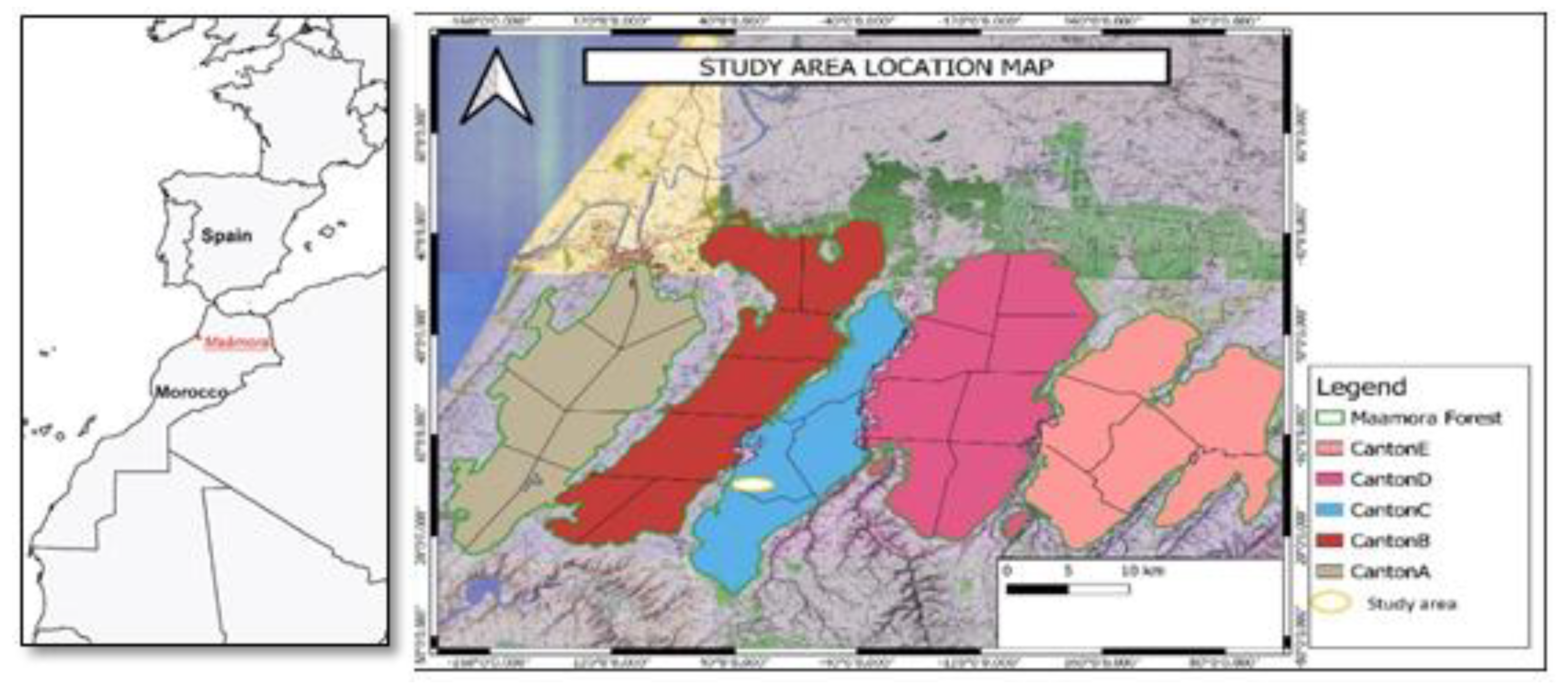
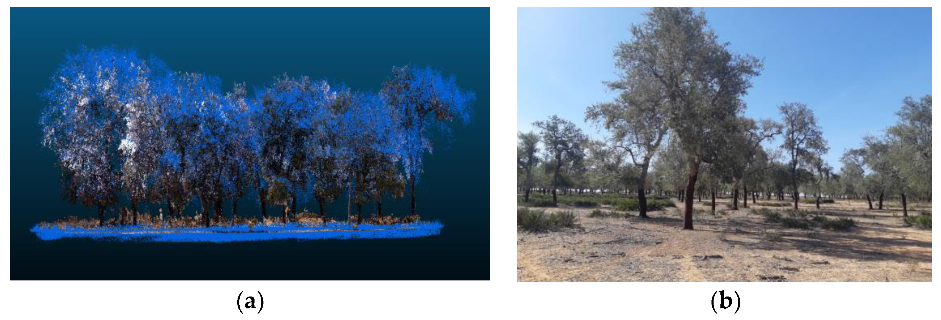
2.1. Study Area
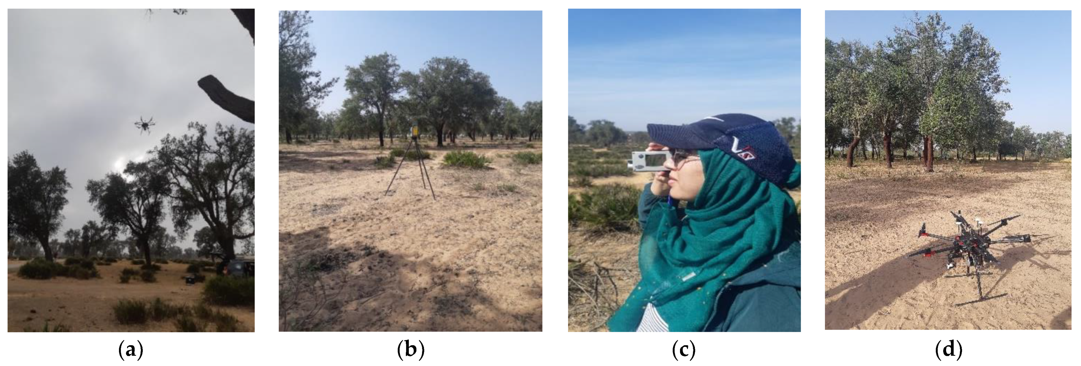
2.2. Data Acquisition
2.2.1. ALS-UAV Data Acquisition
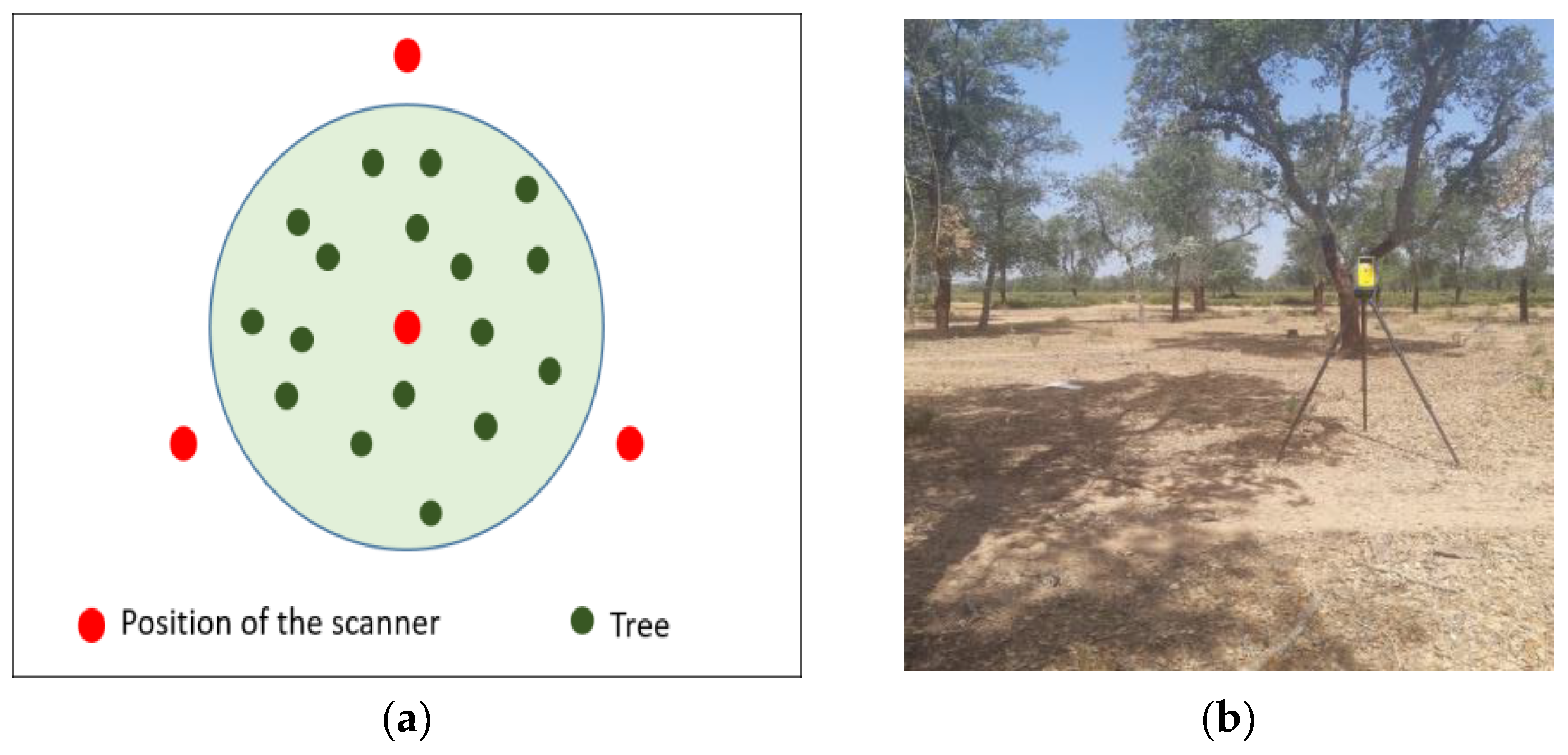
2.2.2. TLS Data Acquisition
2.2.3. Field Data Collection
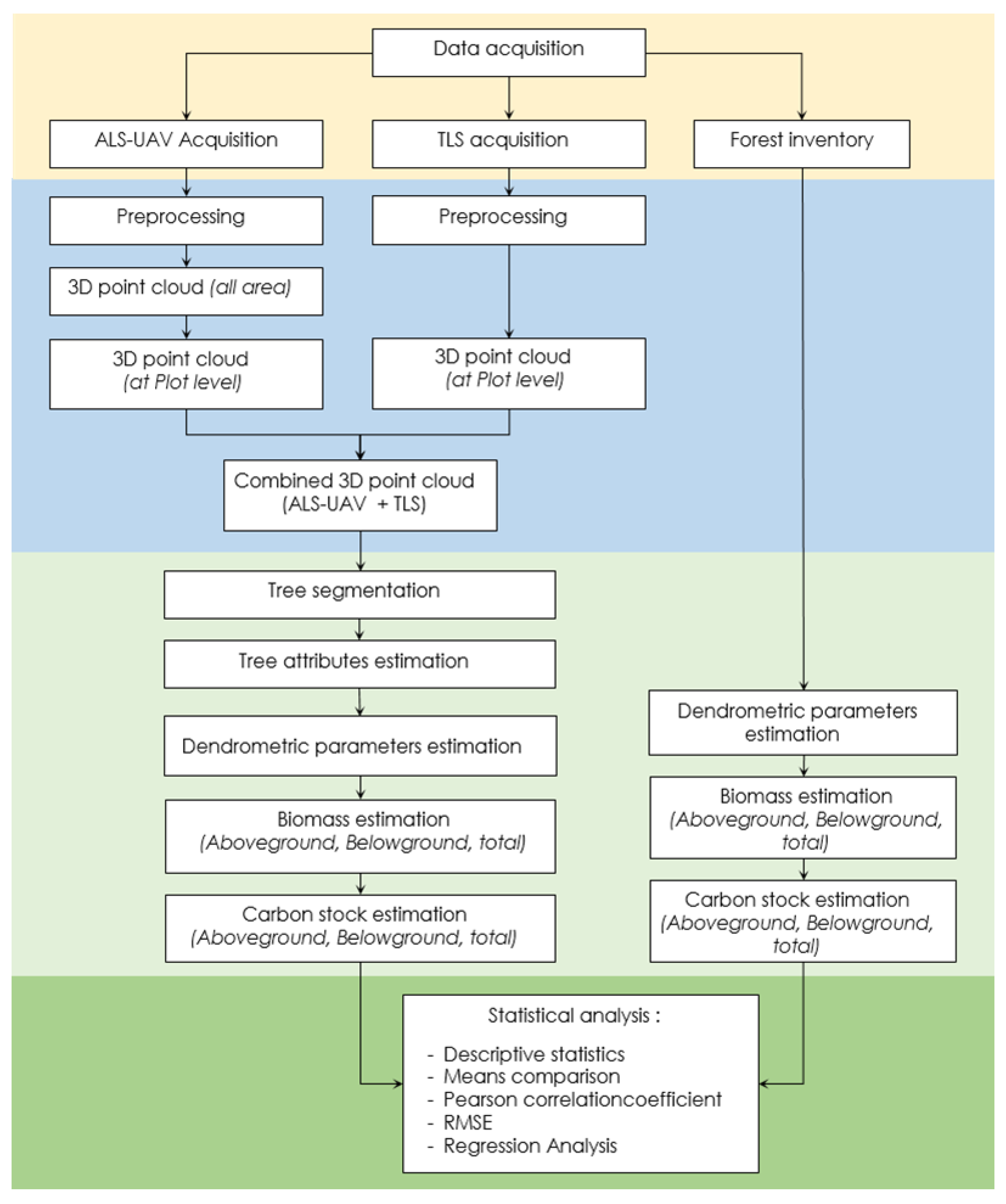
2.3. Data Processing
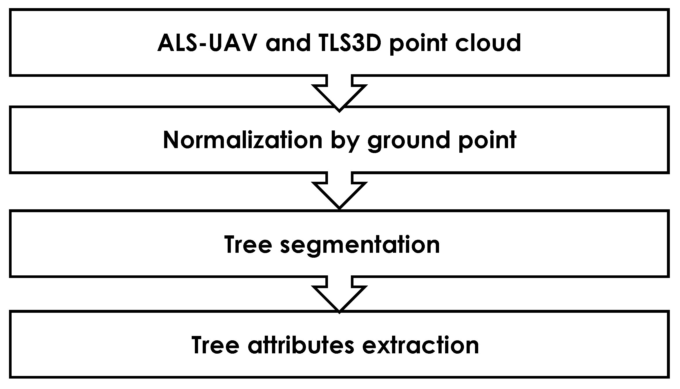
2.3.1. ALS-UAV-TLS Data Pre-Processing and Processing
- Normalization by ground point
- Tree segmentation
- Tree attributes extraction
2.3.2. Field Data Processing
- Model Specifications:
- Criteria for choosing models
- Multiple and adjusted R²—Coefficient of determination is the proportion of the variation in the dependent variable that is predictable from the independent variable(s).
- Residual standard error—The mean square error is the mean of the sum of squared residuals; it measures the average of the squares of the errors. Lower values (closer to zero) indicate better fit.
- AIC—The Akaike information criterion is an estimator of prediction error and thereby relative quality of statistical models for a given set of data.
- BIC—Bayesian information criterion (BIC) is a criterion for model selection among a finite set of models; models with lower BIC are generally preferred.
2.4. Biomass and Carbon Stock Estimation
2.4.1. Biomass Estimation
- Biomass estimation of Stem, Coarse branches, and Cork
- Biomass estimation of medium and small branches and foliage
- Aboveground, belowground, and total biomass estimation
2.4.2. Carbon Stock Estimation
2.5. Statistical Analysis
3. Results
3.1. Relationship between Tree Height and Circumference at 1.30 m
3.2. Statistical Analysis, Relationship, and Regression of Tree Dendrometric Parameters, Biomass, and Carbon Stock
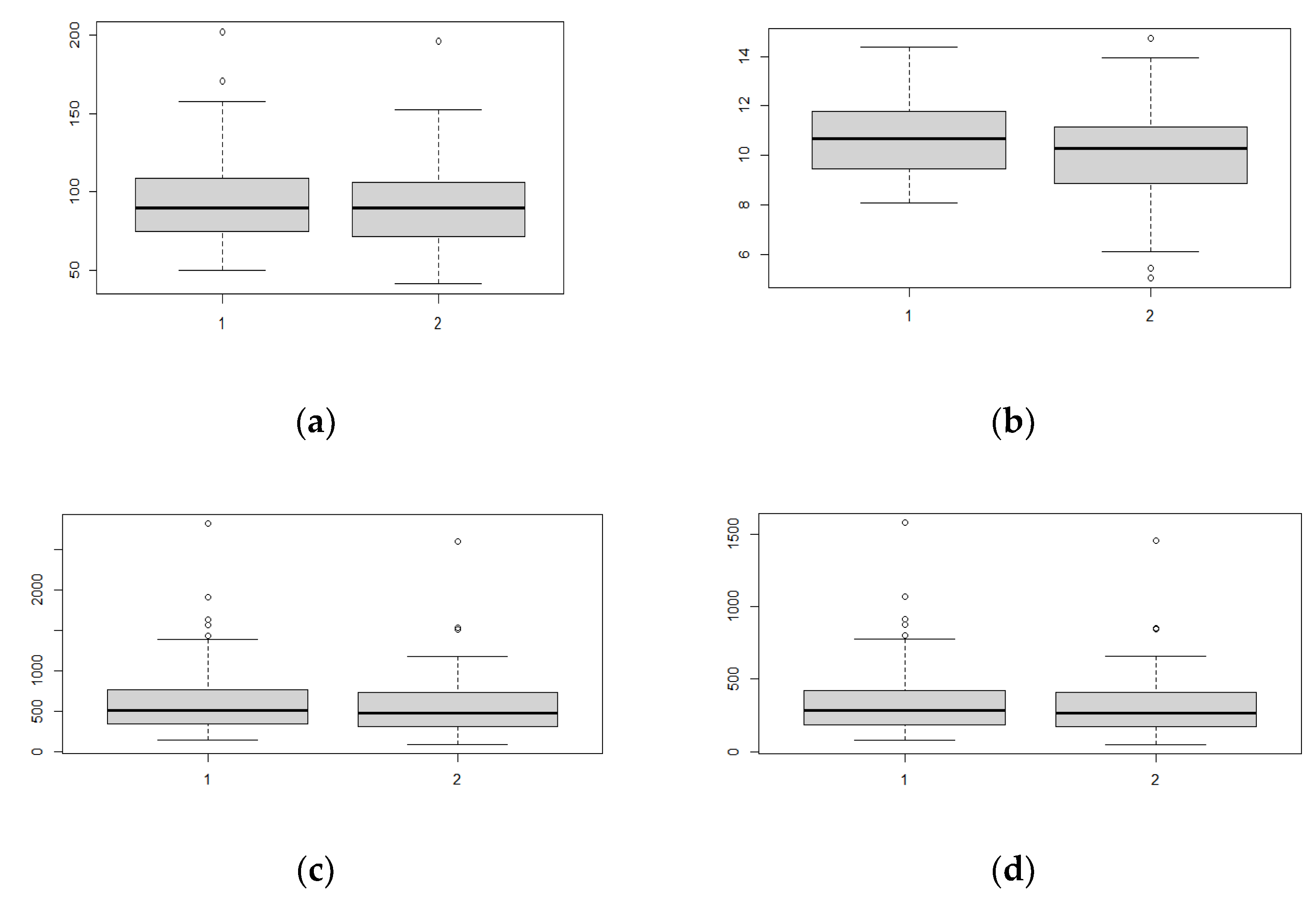
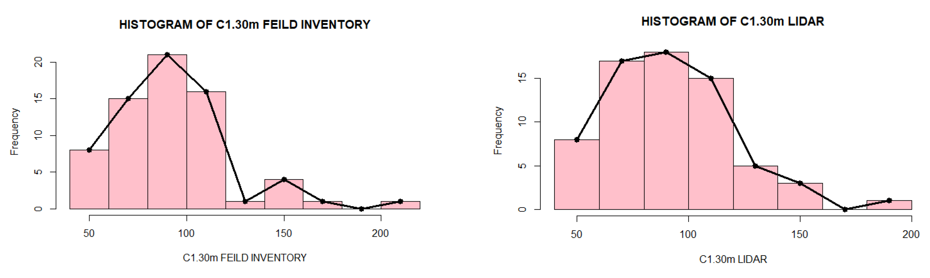
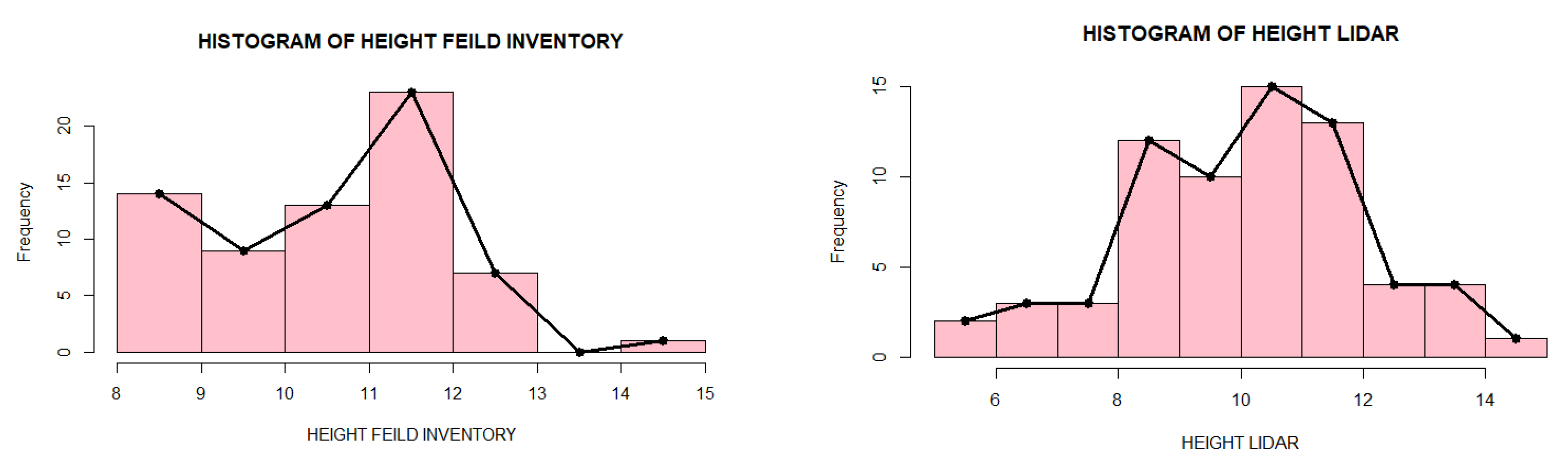
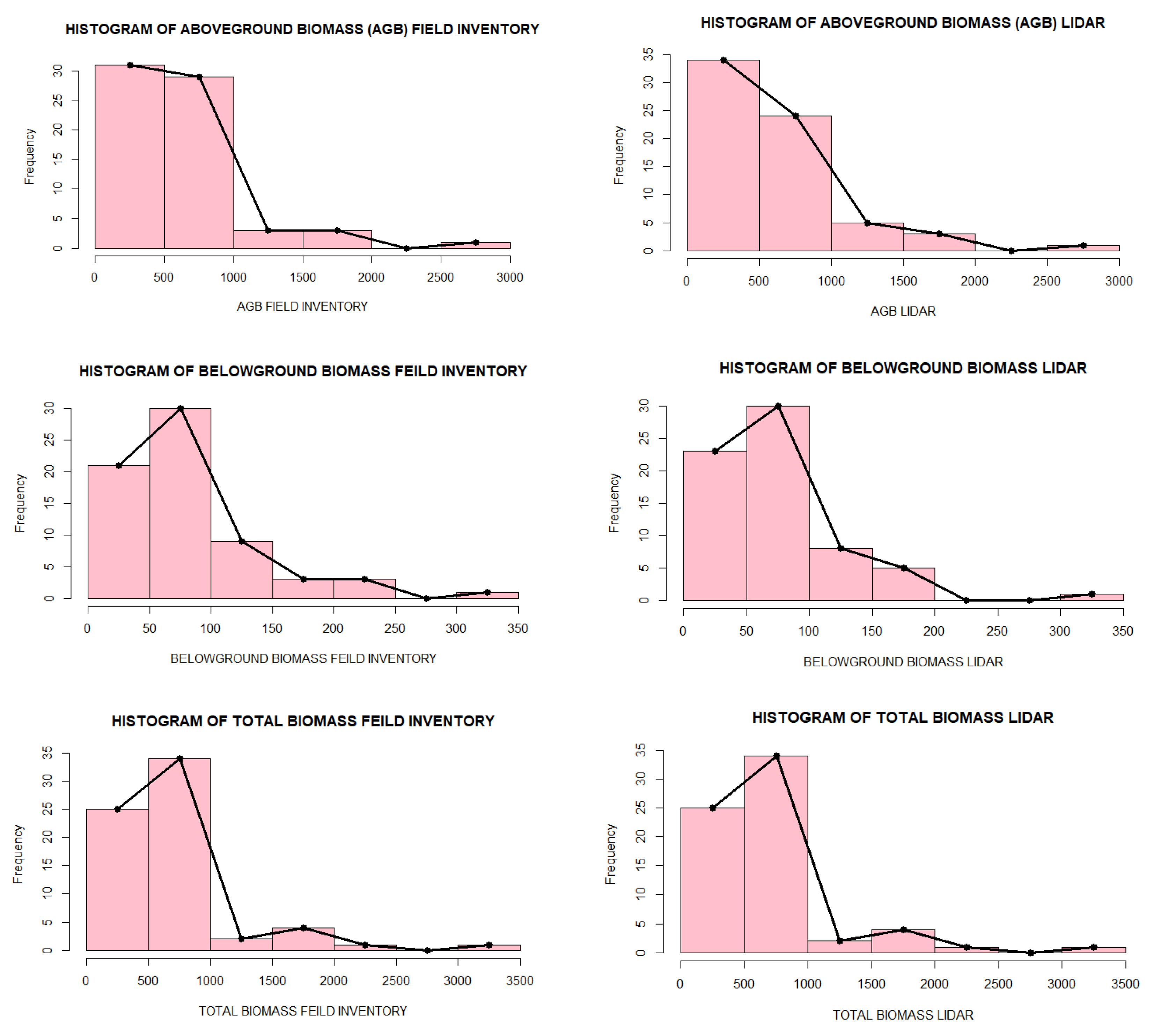
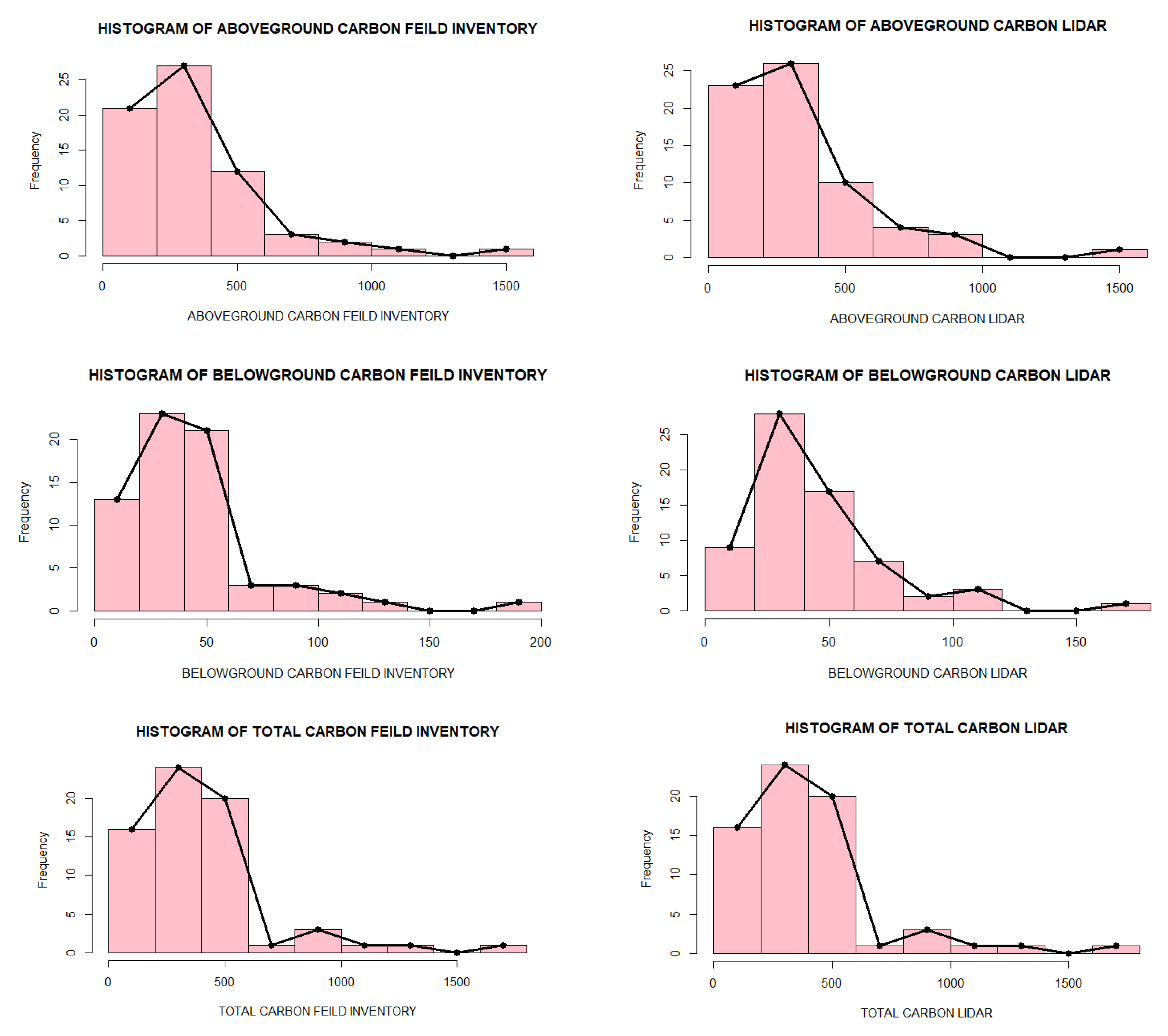
3.2.1. Statistical Analysis and Comparison of Means
- Dendrometric parameters (C1.30m and Tree Height)
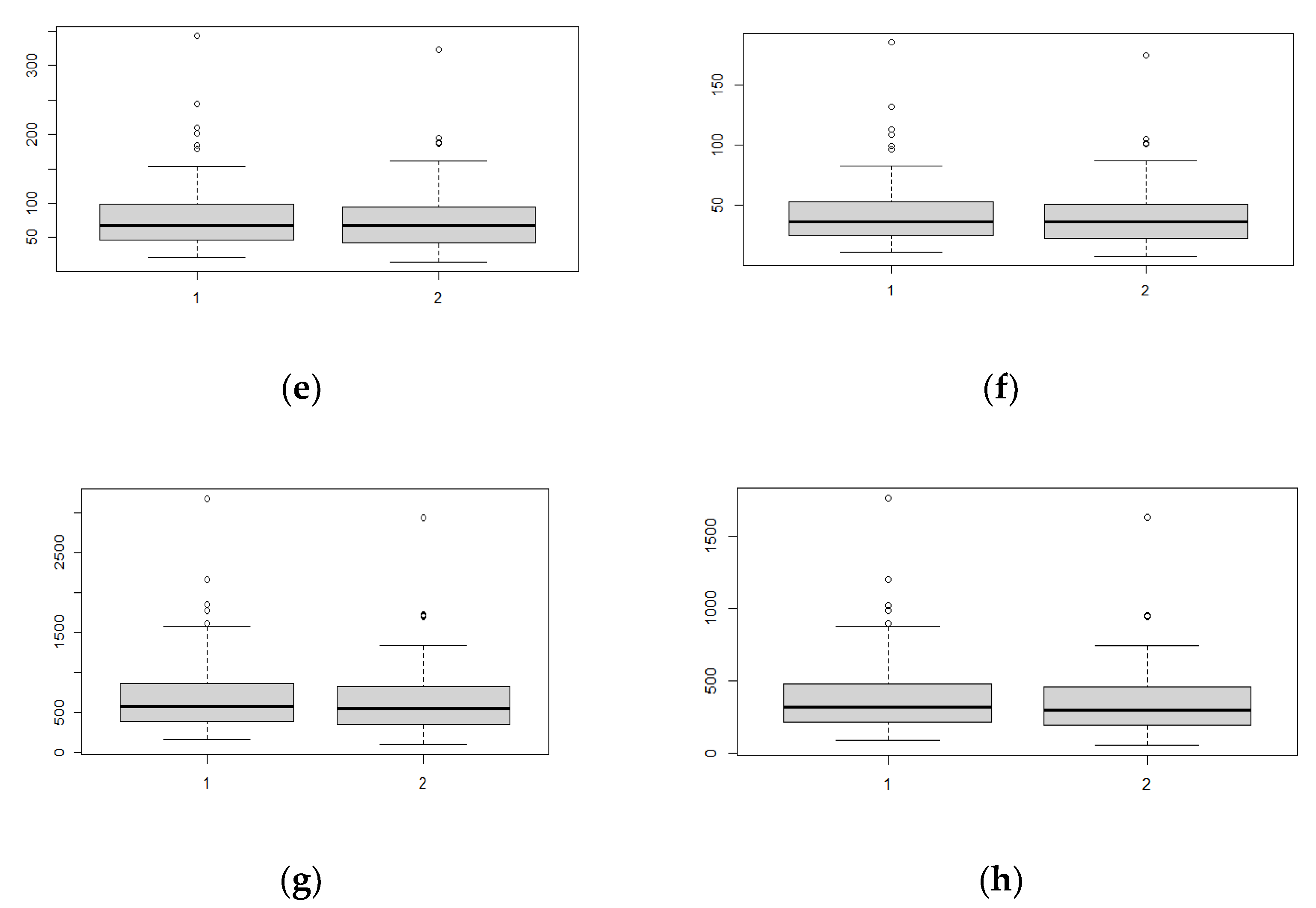
- Aboveground, belowground, and total biomass
- Aboveground, belowground, and total carbon stock
3.2.2. Relationship between Dendrometric Parameters, Biomass, and Carbon Stock of the Two Methods (Pearson Correlation, RMSE and Regression Analysis)
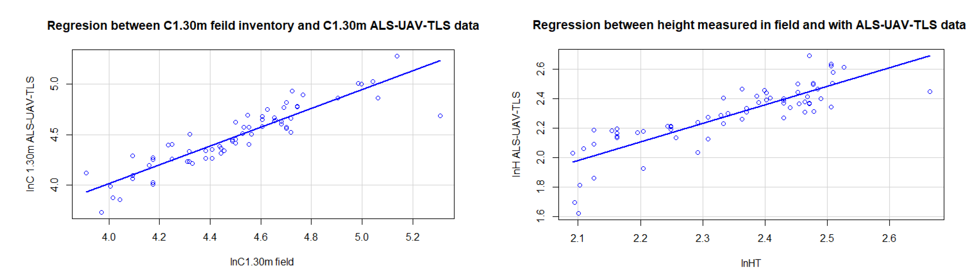
- C1.30m and tree height
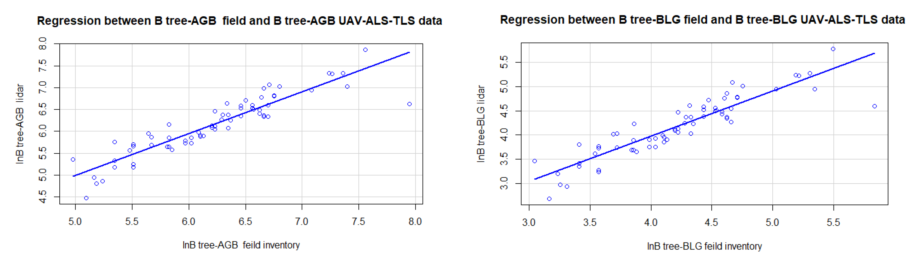
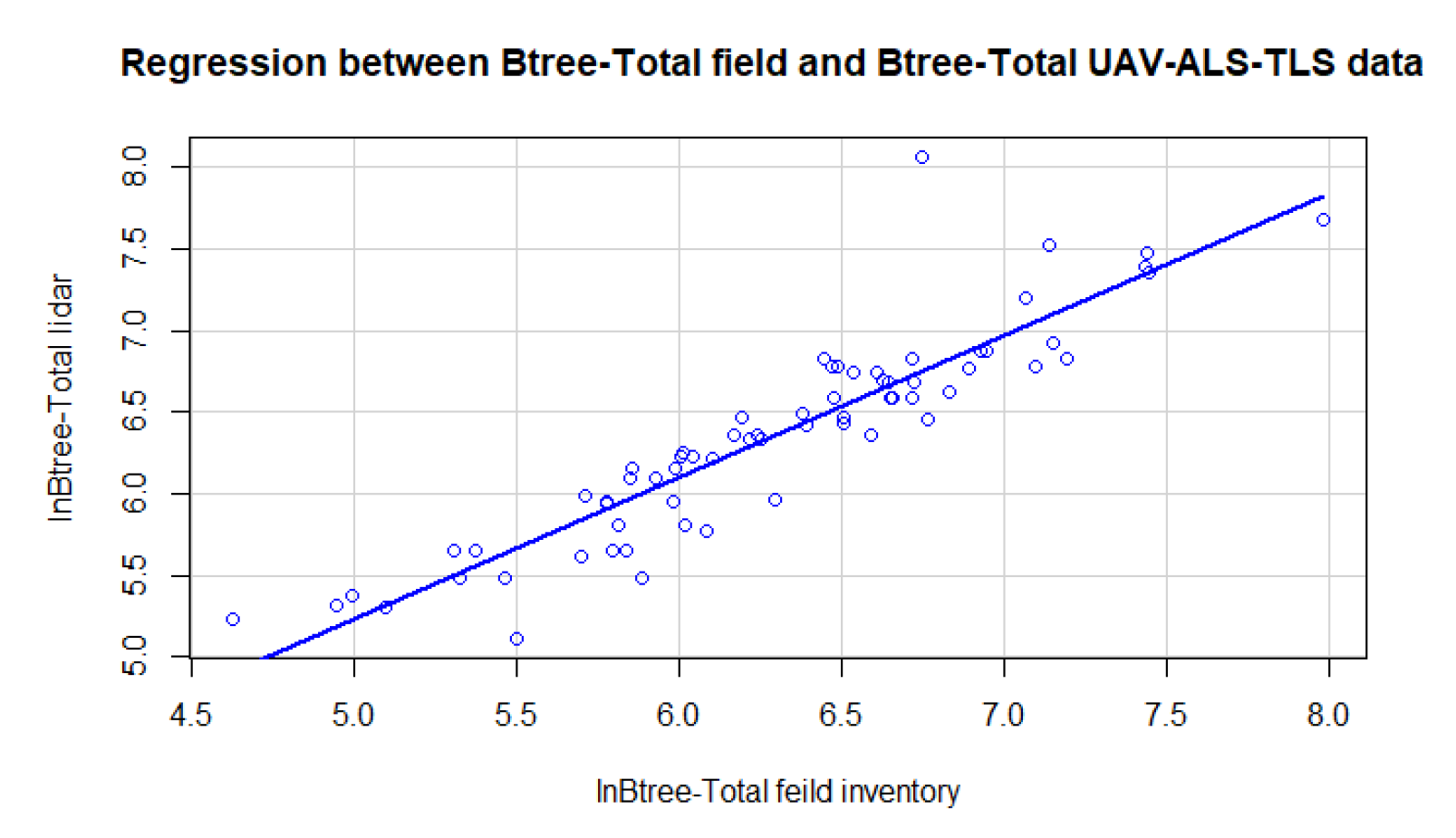
- Aboveground, belowground, and total biomass
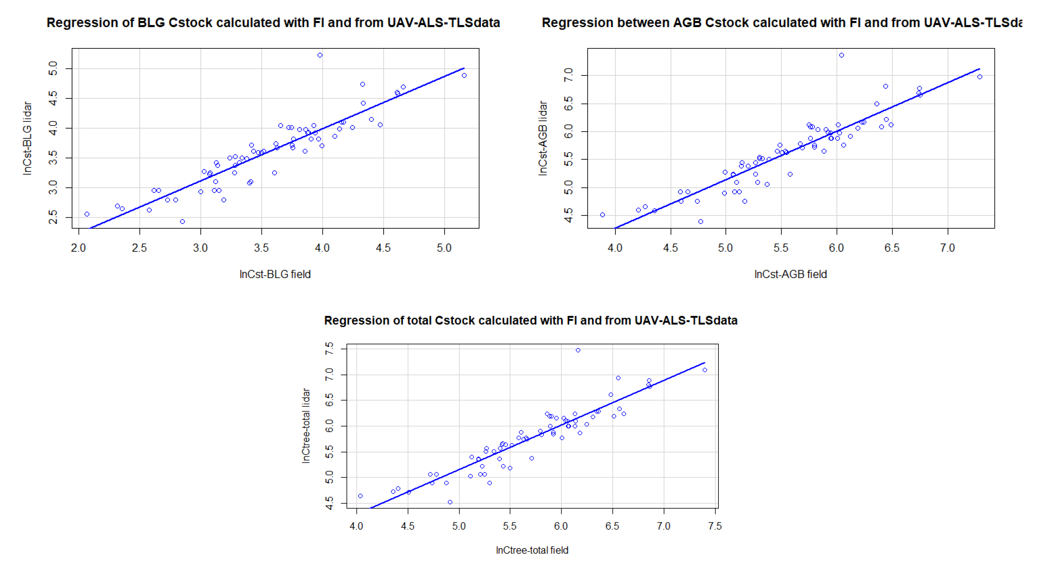
- Aboveground, belowground, and total carbon stock
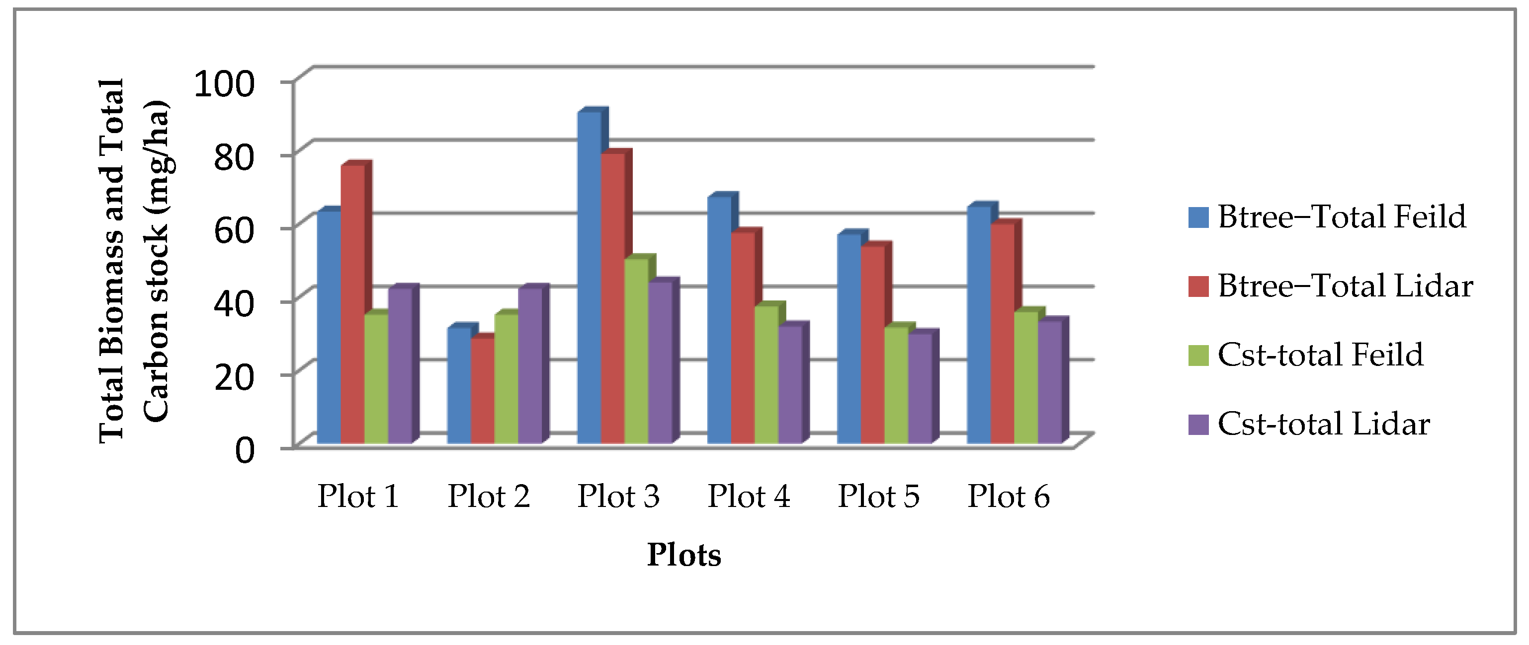
3.3. Analysis at Plot Level of Aboveground, Belowground and Total Biomass and Carbon Stock
4. Discussion
4.1. Dendrometric Parameters (Tree Height and Circumference at 1.30 m)
4.2. Estimation of Aboveground, Belowground, and Total Biomass
4.3. Estimation of Aboveground, belowground, and total Carbon Stock
4.4. Biomass and Carbon Stock in the Cork Oak Stand
5. Conclusions
Author Contributions
Funding
Acknowledgments
Conflicts of Interest
Appendix A

| Specific Tissue Density (kg m−3) | Mean Carbon Concentration (g/kg) | |
|---|---|---|
| Stem and Coarse branches (Ø > 10 cm) | 830 | 560 |
| Cork | 540 | 560 |
| Medium branches (2 ≤ Ø ≤ 10 cm) | - | 540 |
| Small branches (Ø < 2 cm) | - | 530 |
| Foliage | - | 520 |
| Roots | - |
References
- IPCC. Climate Change 2022: Impacts, Adaptation, and Vulnerability. Contribution of Working Group II to the Six Assessment Report of the Intergovernmental Panel on Climate Change. 2022. Available online: https://www.ipcc.ch/report/ar6/wg2/ (accessed on 4 June 2022).
- Friedlingstein, P.; O’Sullivan, M.; Jones, M.W.; Andrew, R.M.; Hauck, J.; Olsen, A.; Peters, G.P.; Peters, W.; Pongratz, J.; Sitch, S.; et al. Global Carbon Budget 2020. Earth Syst. Sci. Data 2020, 12, 3269–3340. [Google Scholar] [CrossRef]
- Harris, N.L.; Gibbs, D.A.; Baccini, A.; Birdsey, R.A.; de Bruin, S.; Farina, M.; Fatoyinbo, L.; Hansen, M.C.; Herold, M.; Houghton, R.A.; et al. Global Maps of Twenty-First Century Forest Carbon Fluxes. Nat. Clim. Chang. 2021, 11, 234–240. [Google Scholar] [CrossRef]
- Watson, R.T.; Noble, I.R.; Bolin, B.; Ravindranath, N.H.; Verardo, D.J.; Dokken, D.J. Land Use, Land-Use Change and Forestry: A Special Report of the Intergovernmental Panel on Climate Change; Cambridge University Press: Cambridge, UK, 2000. [Google Scholar]
- Dixon, R.K.; Winjum, J.K.; Andrasko, K.J.; Lee, J.J.; Schroeder, P.E. Integrated Land-Use Systems: Assessment of Promising Agroforest and Alternative Land-Use Practices to Enhance Carbon Conservation and Sequestration. Clim. Chang. 1994, 27, 71–92. [Google Scholar] [CrossRef]
- Matyssek, R.; Wieser, G.; Calfapietra, C.; de Vries, W.; Dizengremel, P.; Ernst, D.; Jolivet, Y.; Mikkelsen, T.N.; Mohren, G.M.J.; Le Thiec, D.; et al. Forests under Climate Change and Air Pollution: Gaps in Understanding and Future Directions for Research. Environ. Pollut. 2012, 160, 57–65. [Google Scholar] [CrossRef] [PubMed]
- Rappaport, D.I.; Morton, D.C.; Longo, M.; Keller, M.; Dubayah, R.; dos-Santos, M.N. Quantifying Long-Term Changes in Carbon Stocks and Forest Structure from Amazon Forest Degradation. Environ. Res. Lett. 2018, 13, 065013. [Google Scholar] [CrossRef]
- Pandey, A.; Arunachalam, K.; Thadani, R.; Singh, V. Forest Degradation Impacts on Carbon Stocks, Tree Density and Regeneration Status in Banj Oak Forests of Central Himalaya. Ecol. Res. 2020, 35, 208–218. [Google Scholar] [CrossRef]
- Croitoru, L.; Merlo, M. Mediterranean Forest Values. In Valuing Mediterranean Forests: Towards Total Economic Value; CABI Publishing: Wallingford, UK, 2005; pp. 37–68. [Google Scholar]
- Houghton, J. Global Warming: The Complete Briefing; Cambridge University Press: Cambridge, UK, 2009. [Google Scholar]
- Lu, D. The Potential and Challenge of Remote Sensing-based Biomass Estimation. Int. J. Remote Sens. 2006, 27, 1297–1328. [Google Scholar] [CrossRef]
- CDP-Global-Climate-Change-Report-2015. Available online: https://cdn.cdp.net/cdp-production/cms/reports/documents/000/000/578/original/CDP-global-climate-change-report-2015.pdf (accessed on 4 June 2022).
- Vashum, K.T. Methods to Estimate Above-Ground Biomass and Carbon Stock in Natural Forests—A Review. J. Ecosyst. Ecography 2012, 2, 1–7. [Google Scholar] [CrossRef]
- Liu, C.; Lu, M.; Cui, J.; Li, B.; Fang, C. Effects of Straw Carbon Input on Carbon Dynamics in Agricultural Soils: A Meta-Analysis. Glob. Change Biol. 2014, 20, 1366–1381. [Google Scholar] [CrossRef] [PubMed]
- McGovern, M.; Pasher, J. Canadian Urban Tree Canopy Cover and Carbon Sequestration Status and Change 1990–2012. Urban For. Urban Green. 2016, 20, 227–232. [Google Scholar] [CrossRef]
- Myeong, S.; Nowak, D.J.; Duggin, M.J. A Temporal Analysis of Urban Forest Carbon Storage Using Remote Sensing. Remote Sens. Environ. 2006, 101, 277–282. [Google Scholar] [CrossRef]
- Shen, H.; Huang, L.; Zhang, L.; Wu, P.; Zeng, C. Long-Term and Fine-Scale Satellite Monitoring of the Urban Heat Island Effect by the Fusion of Multi-Temporal and Multi-Sensor Remote Sensed Data: A 26-Year Case Study of the City of Wuhan in China. Remote Sens. Environ. 2016, 172, 109–125. [Google Scholar] [CrossRef]
- Jong, S.M.D.; Pebesma, E.J.; Lacaze, B. Above-Ground Biomass Assessment of Mediterranean Forests Using Airborne Imaging Spectrometry: The DAIS Peyne Experiment. Int. J. Remote Sens. 2003, 24, 1505–1520. [Google Scholar] [CrossRef]
- Raciti, S.M.; Hutyra, L.R.; Newell, J.D. Mapping Carbon Storage in Urban Trees with Multi-Source Remote Sensing Data: Relationships between Biomass, Land Use, and Demographics in Boston Neighborhoods. Sci. Total Environ. 2014, 500–501, 72–83. [Google Scholar] [CrossRef] [PubMed]
- Thenkabail, P.S.; Stucky, N.; Griscom, B.W.; Ashton, M.S.; Diels, J.; van der Meer, B.; Enclona, E. Biomass Estimations and Carbon Stock Calculations in the Oil Palm Plantations of African Derived Savannas Using IKONOS Data. Int. J. Remote Sens. 2004, 25, 5447–5472. [Google Scholar] [CrossRef]
- Koch, B. Status and Future of Laser Scanning, Synthetic Aperture Radar and Hyperspectral Remote Sensing Data for Forest Biomass Assessment. ISPRS J. Photogramm. Remote Sens. 2010, 65, 581–590. [Google Scholar] [CrossRef]
- Stephens, P.R.; Kimberley, M.O.; Beets, P.N.; Paul, T.S.H.; Searles, N.; Bell, A.; Brack, C.; Broadley, J. Airborne Scanning LiDAR in a Double Sampling Forest Carbon Inventory. Remote Sens. Environ. 2012, 117, 348–357. [Google Scholar] [CrossRef]
- Fatoyinbo, T.; Feliciano, E.A.; Lagomasino, D.; Lee, S.K.; Trettin, C. Estimating Mangrove Aboveground Biomass from Airborne LiDAR Data: A Case Study from the Zambezi River Delta. Environ. Res. Lett. 2018, 13, 025012. [Google Scholar] [CrossRef]
- Hickey, S.M.; Callow, N.J.; Phinn, S.; Lovelock, C.E.; Duarte, C.M. Spatial Complexities in Aboveground Carbon Stocks of a Semi-Arid Mangrove Community: A Remote Sensing Height-Biomass-Carbon Approach. Estuar. Coast. Shelf Sci. 2018, 200, 194–201. [Google Scholar] [CrossRef]
- Wang, D.; Wan, B.; Liu, J.; Su, Y.; Guo, Q.; Qiu, P.; Wu, X. Estimating aboveground biomass of the mangrove forests on northeast Hainan Island in China using an upscaling method from field plots, UAV-LiDAR data and Sentinel-2 imagery. Int. J. Appl. Earth Obs. Geoinf. 2020, 85, 101986. [Google Scholar] [CrossRef]
- De Almeida, C.T.; Galvao, L.S.; Ometto, J.P.H.B.; Jacon, A.D.; de Souza Pereira, F.R.; Sato, L.Y.; Lopes, A.P.; de Alencastro Graça, P.M.L.; de Jesus Silva, C.V.; Ferreira-Ferreira, J.; et al. Combining LiDAR and Hyperspectral Data for Aboveground Biomass Modeling in the Brazilian Amazon Using Different Regression Algorithms. Remote Sens. Environ. 2019, 232, 111323. [Google Scholar] [CrossRef]
- Longo, M.; Keller, M.; dos-Santos, M.N.; Leitold, V.; Pinagé, E.R.; Baccini, A.; Saatchi, S.; Nogueira, E.M.; Batistella, M.; Morton, D.C. Aboveground Biomass Variability across Intact and Degraded Forests in the Brazilian Amazon. Glob. Biogeochem. Cycles 2016, 30, 1639–1660. [Google Scholar] [CrossRef]
- Tyukavina, A.; Baccini, A.; Hansen, M.C.; Potapov, P.V.; Stehman, S.V.; Houghton, R.A.; Krylov, A.M.; Turubanova, S.; Goetz, S.J. Aboveground Carbon Loss in Natural and Managed Tropical Forests from 2000 to 2012. Environ. Res. Lett. 2015, 10, 074002. [Google Scholar] [CrossRef]
- Wang, V.; Gao, J.; Schwendenmann, L. Assessing Changes of Urban Vegetation Cover and Aboveground Carbon Stocks Using LiDAR and Landsat Imagery Data in Auckland, New Zealand. Int. J. Remote Sens. 2020, 41, 2140–2158. [Google Scholar] [CrossRef]
- Fadil, S.; Sebari, I.; Bouhaloua, M.; Kadi, K.A.E. Opportunités d’utilisation de la technologie drone au niveau des écosystèmes forestiers. Rev. Maroc. Des Sci. Agron. Vét 2020, 8. Available online: https://www.agrimaroc.org/index.php/Actes_IAVH2/article/view/888 (accessed on 4 June 2022).
- Mtui, Y.P. Tropical Rainforest above Ground Biomass and Carbon Stock Estimation for Upper and Lower Canopies Using Terrestrial Laser Scanner and Canopy Height Model from Unmanned Aerial Vehicle (UAV) Imagery in Ayer-Hitam, Malaysia. Master’s Thesis, University of Twente, Enschede, The Netherlands, 2017; p. 73. [Google Scholar]
- Fernandes, M.R.; Aguiar, F.C.; Martins, M.J.; Rico, N.; Ferreira, M.T.; Correia, A.C. Carbon Stock Estimations in a Mediterranean Riparian Forest: A Case Study Combining Field Data and UAV Imagery. Forests 2020, 11, 376. [Google Scholar] [CrossRef]
- Wirasatriya, A.; Pribadi, R.; Iryanthony, S.B.; Maslukah, L.; Sugianto, D.N.; Helmi, M.; Ananta, R.R.; Adi, N.S.; Kepel, T.L.; Ati, R.N.A.; et al. Mangrove Above-Ground Biomass and Carbon Stock in the Karimunjawa-Kemujan Islands Estimated from Unmanned Aerial Vehicle-Imagery. Sustainability 2022, 14, 706. [Google Scholar] [CrossRef]
- Belghazi, B.; Ezzahiri, M.; Amhajar, M.; Benzyane, M. Régénération artificielle du chêne-liège dans la forêt de la Mâamora (Maroc). For. Méditerr. 2001, 22, 253–261. [Google Scholar]
- Aafi, A.; Achhal El Kadmiri, A.; Benabid, A.; Rochdi, M. Richesse et diversité floristique de la subéraie de la Mamora (Maroc). Acta Bot. Malacit. 2005, 30, 127–138. [Google Scholar] [CrossRef]
- Aafi, A. Etude de la Diversité Floristique de L'écosystème de Chêne-Liège de la Forêt de la Mamora; Institut Agronomique et Vétérinaire Hassan II: Rabat, Morocco, 2007. [Google Scholar]
- Noumonvi, K.D.; Mounir, F.; Belghazi, B. Spatial Multi-Criteria Based Analysis to Assess Dynamics and Vulnerability of Forest Ecosystems to Global Changes: Case of Maamora Forest-Morocco. OALib 2017, 4, 1–16. [Google Scholar] [CrossRef]
- Kankare, V.; Liang, X.; Vastaranta, M.; Yu, X.; Holopainen, M.; Hyyppä, J. Diameter Distribution Estimation with Laser Scanning Based Multisource Single Tree Inventory. ISPRS J. Photogramm. Remote Sens. 2015, 108, 161–171. [Google Scholar] [CrossRef]
- Tao, S.; Wu, F.; Guo, Q.; Wang, Y.; Li, W.; Xue, B.; Hu, X.; Li, P.; Tian, D.; Li, C.; et al. Segmenting tree crowns from terrestrial and mobile LiDAR data by 2 exploring ecological theories. ISPRS J. Photogramm. Remote Sens. 2015, 110, 66–76. [Google Scholar] [CrossRef]
- Oubrahim, H.; Boulmane, M.; Bakker, M.; Augusto, L.; Halim, M. Carbon Storage in Degraded Cork Oak (Quercus Suber) Forests on Flat Lowlands in Morocco. IForest—Biogeosci. For. 2016, 9, 125–137. [Google Scholar] [CrossRef]
- Makhloufi, M.; Abourouh, M.; El Harchaoui, H. Structure Du Peuplement, Tarifs de Cubage et Essai de Traitements Sylvicoles Dans La Subéraie de Chefchaouen. In Annales de la Recherche Forestière au Maroc; National Center of Forestery Research: Rabat, Morocco, 2008; Volume 39, pp. 175–177. [Google Scholar]
- Ruiz-Peinado Gertrudix, R.; Montero, G.; Del Rio, M. Biomass Models to Estimate Carbon Stocks for Hardwood Tree Species. For. Syst. 2012, 21, 42. [Google Scholar] [CrossRef]
- Ma, K.; Chen, Z.; Fu, L.; Tian, W.; Jiang, F.; Yi, J.; Du, Z.; Sun, H. Performance and Sensitivity of Individual Tree Segmentation Methods for UAV-LiDAR in Multiple Forest Types. Remote Sens. 2022, 14, 298. [Google Scholar] [CrossRef]
- Maan, G.S.; Singh, C.K.; Singh, M.K.; Nagarajan, B. Tree Species Biomass and Carbon Stock Measurement Using Ground Based-LiDAR. Geocarto Int. 2015, 30, 293–310. [Google Scholar] [CrossRef]
- Mohd Zaki, N.A.; Abd Latif, Z.; Zainal, M.Z. Aboveground biomass and carbon stock estimation using double sampling approach and remotely-sensed data. J. Teknol. 2016, 78. [Google Scholar] [CrossRef][Green Version]
- Qin, S.; Nie, S.; Guan, Y.; Zhang, D.; Wang, C.; Zhang, X. Forest Emissions Reduction Assessment Using Airborne LiDAR for Biomass Estimation. Resour. Conserv. Recycl. 2022, 181, 106224. [Google Scholar] [CrossRef]
- Zhao, Y.; Ma, Y.; Quackenbush, L.J.; Zhen, Z. Estimation of Individual Tree Biomass in Natural Secondary Forests Based on ALS Data and WorldView-3 Imagery. Remote Sens. 2022, 14, 271. [Google Scholar] [CrossRef]
- Boulmane, M.; Makhloufi, M.; Bouillet, J.-P.; Saint-André, L.; Satrani, B.; Halim, M.; Elantry-Tazi, S. Estimation du stock de carbone organique dans la chênaie verte du Moyen Atlas marocain. Acta Bot. Gallica 2010, 157, 451–467. [Google Scholar] [CrossRef]
- MacDicken, K.G. A Guide to Monitoring Carbon Storage in Forestry and Agroforestry Projects. 1997, p. 91. Available online: https://agris.fao.org/agris-search/search.do?recordID=XF2015020398 (accessed on 4 June 2022).


| Models | Models’ Equations |
|---|---|
| Model 1 | Linear simple model: H = b0 + b1 C 1.30m |
| Model 2 | Allometric model (2nd degree): H = b0 + b1 C 1.30m+ b2 C² 1.30m |
| Model 3 | Allometric model (3nd degree): H = b0 + b1 C 1.30m + b2 C² 1.30m + b3 C3 1.30m |
| Model 4 | Allometric model (4th degree): H = b0 + b1 C 1.30m + b2 C² 1.30m + b3 C3 1.30m + b4 C4 1.30m |
| Model 5 | Allometric model (5th degree): H = b0 + b1 C 1.30m + b2 C² 1.30m + b3 C3 1.30m + b4 C4 1.30m + b5 C5 1.30m |
| Model 6 | Logarithmic model: lnH = a0 + a1 lnC 1.30m |
| Models | Multiple R² | Adjusted R² | Residual Standard Error | AIC | BIC |
|---|---|---|---|---|---|
| Model 1—Linear simple model | 0.66 | 0.65 | 1.198 | 130.40 | 125.48 |
| Model 2—Allometric model (2nd degree) | 0.67 | 0.65 | 1.194 | 126.20 | 132.75 |
| Model 3—Allometric model (3rd degree) | 0.71 | 0.68 | 1.147 | 124.04 | 132.23 |
| Model 4—Allometric model (4th degree) | 0.73 | 0.69 | 1.124 | 123.38 | 133.21 |
| Model 5—Allometric model (5th degree) | 0.75 | 0.71 | 1.087 | 121.63 | 133.09 |
| Model 6—Logarithmic model | 0.66 | 0.65 | 0.098 | −64.47 | −59.55 |
| Min | 1st Qu | Median | Mean | 3rd Qu | Max | ||
|---|---|---|---|---|---|---|---|
| C 1.30m (cm) | Field measurements | 50.00 | 74.75 | 90.00 | 94.16 | 108.50 | 202.00 |
| ALS-UAV-TLS | 41.76 | 71.46 | 90.12 | 92.32 | 106.05 | 195.94 | |
| Height field (m) | Field measurements | 8.10 | 9.45 | 10.69 | 10.55 | 11.77 | 14.36 |
| ALS-UAV-TLS | 5.07 | 8.89 | 10.30 | 10.08 | 11.17 | 14.73 | |
| Btree−AGB field (kg) | Field measurements | 145.5 | 336.1 | 506.9 | 619.9 | 759.8 | 2826.9 |
| ALS-UAV-TLS | 87.81 | 306.20 | 474.54 | 586.80 | 729.20 | 2609.16 | |
| Btree−BLG field (kg) | Field measurements | 21.02 | 46.98 | 68.11 | 81.75 | 98.98 | 343.08 |
| ALS-UAV-TLS | 14.66 | 42.94 | 68.28 | 78.46 | 94.56 | 322.79 | |
| Btree-total field (kg) | Field measurements | 166.5 | 383.1 | 575.0 | 701.7 | 858.8 | 3169.9 |
| ALS-UAV-TLS | 102.5 | 348.7 | 542.8 | 665.3 | 825.1 | 2932.0 | |
| Cst− AGB field (kg) | Field measurements | 80.96 | 187.34 | 282.68 | 345.86 | 423.89 | 1579.41 |
| ALS-UAV-TLS | 48.89 | 170.62 | 264.74 | 327.39 | 406.82 | 1457.79 | |
| Cst−BLG field (kg) | Field measurements | 11.35 | 25.37 | 36.78 | 44.14 | 53.45 | 185.26 |
| ALS-UAV-TLS | 7.91 | 23.18 | 36.87 | 42.36 | 51.06 | 174.30 | |
| Ctree-total field (kg) | Field measurements | 92.31 | 212.71 | 319.46 | 390.00 | 477.34 | 1764.68 |
| ALS-UAV-TLS | 56.81 | 193.59 | 301.61 | 369.75 | 458.60 | 1632.10 |
| Shapiro-Test | |||
|---|---|---|---|
| W | p-Value | ||
| C1.30m (cm) | Field measurements | 0.9181 | 0.0002995 |
| ALS-UAV-TLS | 0.95394 | 0.0145 | |
| Height field (m) | Field measurements | 0.94178 | 0.003553 |
| ALS-UAV-TLS | 0.98596 | 0.6532 | |
| B tree−AGB field (kg) | Field measurements | 0.7748 | 9.217 × 10⁻⁹ |
| ALS-UAV-TLS | 0.81877 | 1.269 × 10⁻⁷ | |
| B tree−BLG field (kg) | Field measurements | 0.78662 | 1.804 × 10⁻⁸ |
| ALS-UAV-TLS | 0.83436 | 3.529 × 10⁻⁷ | |
| B tree-total field (kg) | Field measurements | 0.77616 | 9.944 × 10⁻⁹ |
| ALS-UAV-TLS | 0.82049 | 1.417 × 10⁻⁷ | |
| Cst− AGB field (kg) | Field measurements | 0.77443 | 9.03 × 10⁻⁹ |
| ALS-UAV-TLS | 0.81842 | 1.241 × 10⁻⁷ | |
| C st−BLG field (kg) | Field measurements | 0.78662 | 1.804 × 10⁻⁸ |
| ALS-UAV-TLS | 0.83436 | 3.529 × 10⁻⁷ | |
| C tree-total field (kg) | Field measurements | 0.77579 | 9.741 × 10⁻⁹ |
| ALS-UAV-TLS | 0.82013 | 1.384 × 10⁻⁷ | |
| Wilcoxon-test | |||
| Field C1.30m (cm)/ C1.30m ALS-UAV-TLS (cm) | 2308 | 0.7792 | |
| Field height (m)/Height ALS-UAV-TLS (m) | 2605 | 0.1091 | |
| B tree−AGB field (kg)/B tree−AGB ALS-UAV-TLS (kg) | 2335 | 0.6888 | |
| B tree−BLG field (kg)/B tree−BLG ALS-UAV-TLS (kg) | 2308 | 0.7792 | |
| B st−total field (kg)/B st−total ALS-UAV-TLS (kg) | 2328 | 0.7119 | |
| C tree−AGB field (kg)/C tree−AGB ALS-UAV-TLS (kg) | 2335 | 0.6888 | |
| C tree−BLG field (kg)/C tree−BLG ALS-UAV-TLS (kg) | 2308 | 0.7792 | |
| C st−total field (kg)/C st−total ALS-UAV-TLS (kg) | 2329 | 0.7085 | |
| Pearson Coef | RMSE | |
|---|---|---|
| C1.30m (cm) field/C1.30m ALS-UAV-TLS (cm) | 0.86 | 1.84 |
| Height (m) field/Height ALS-UAV-TLS (m) | 0.83 | 0.47 |
| B tree−AGB field (kg)/B tree−AGB ALS-UAV-TLS (kg) | 0.77 | 33.11 |
| B tree−BLG field (kg)/B tree−BLG ALS-UAV-TLS (kg) | 0.78 | 3.29 |
| B tree−total field (kg)/B tree−total ALS-UAV-TLS (kg) | 0.77 | 36.40 |
| C tree−AGB field (kg)/C tree−AGB ALS-UAV-TLS (kg) | 0.77 | 18.47 |
| C tree−BLG field (kg)/C tree−BLG ALS-UAV-TLS (kg) | 0.78 | 1.77 |
| C st−total field (kg)/C st−total ALS-UAV-TLS (kg) | 0.77 | 20.24 |
| Dendrometric Parameters | ||||
|---|---|---|---|---|
| Multiple R2 | Adjusted R2 | |||
| lnC1.30m field/lnC1.30m ALS-UAV-TLS | 0.818 | 0.815 | ||
| lnHeight field/lnHeight ALS-UAV-TLS | 0.712 | 0.708 | ||
| Estimate | Std. Error | t Value | Pr(>|t|) | |
| Intercept1 | 0.28266 | 0.24605 | 1.149 | 0.255 |
| lnC1.30m field | 0.93247 | 0.05455 | 17.093 | <2 × 10⁻¹⁶ *** |
| Intercept2 | −0.65355 | 0.23238 | −2.812 | 0.0065 ** |
| lnHeight field | 1.25423 | 0.09885 | 12.689 | <2 × 10⁻¹⁶ *** |
| Aboveground, belowground, and total Biomass | ||||
| Multiple R2 | Adjusted R2 | |||
| lnB tree−AGB field/lnB tree−AGB ALS-UAV-TLS | 0.833 | 0.831 | ||
| lnB tree−BLG field/lnB tree−BLG ALS-UAV-TLS | 0.818 | 0.8152 | ||
| lnB tree−total field /lnB tree−total ALS-UAV-TLS | 0.832 | 0.829 | ||
| Estimate | Std. Error | t value | Pr(>|t|) | |
| Intercept1 | 0.18394 | 0.33292 | 0.553 | 0.583 |
| lnB tree−AGB field | 0.96027 | 0.05322 | 18.044 | <2 × 10⁻¹⁶ *** |
| Intercept2 | 0.24263 | 0.23259 | 1.043 | 0.301 |
| lnB tree−BLG field | 0.93247 | 0.05455 | 17.093 | <2 × 10⁻¹⁶ *** |
| Intercept3 | 30.21400 | 0.34009 | 0.629 | 0.531 |
| lnB tree−total field | 0.95675 | 0.05329 | 17.953 | <2 × 10⁻¹⁶ *** |
| Aboveground, belowground, and total carbon stock | ||||
| Multiple R2 | Adjusted R2 | |||
| lnC tree−AGB field/lnC tree−AGB ALS-UAV-TLS | 0.8335 | 0.831 | ||
| lnC tree−BLG field/lnC tree−BLG ALS-UAV-TLS | 0.712 | 0.708 | ||
| lnC st−total field/lnC st−total ALS-UAV-TLS | 0.8321 | 0.8296 | ||
| Estimate | Std. Error | t value | Pr(>|t|) | |
| Intercept1 | 0.16194 | 0.30202 | 0.536 | 0.594 |
| lnC tree−AGB field | 0.96006 | 0.05322 | 18.040 | <2 × 10⁻¹⁶ *** |
| Intercept2 | 0.20102 | 0.19935 | 1.008 | 0.317 |
| lnC tree−BLG field | 0.93247 | 0.05455 | 17.093 | <2 × 10⁻¹⁶ *** |
| Intercept3 | 0.18904 | 0.30893 | 0.612 | 0.543 |
| lnC st−total field | 0.95667 | 0.05329 | 17.951 | <2 × 10⁻¹⁶ *** |
| Btree−AGB Feild | Btree-BLG Feild | Btree−Total Field | Cst-AGB Feild | Cst−BLG Feild | Cst-total Feild | Btree−AGB Lidar | Btree-BLG Lidar | Btree−Total Lidar | Cst-AGB Lidar | Cst−BLG Lidar | Cst-total Lidar | |
|---|---|---|---|---|---|---|---|---|---|---|---|---|
| Plot 1 | 56.02 | 7.31 | 63.33 | 31.26 | 3.94 | 35.21 | 67.16 | 8.73 | 75.89 | 37.49 | 4.71 | 42.20 |
| Plot 2 | 27.86 | 3.69 | 31.55 | 15.54 | 3.94 | 35.21 | 25.26 | 3.44 | 28.70 | 37.49 | 4.71 | 42.20 |
| Plot 3 | 80.19 | 10.26 | 90.45 | 44.76 | 5.54 | 50.30 | 69.95 | 9.16 | 79.10 | 39.04 | 4.94 | 43.98 |
| Plot 4 | 59.45 | 7.81 | 67.26 | 33.18 | 4.22 | 37.40 | 50.71 | 6.79 | 57.51 | 28.30 | 3.67 | 31.97 |
| Plot 5 | 50.19 | 6.86 | 57.05 | 27.98 | 3.71 | 31.68 | 47.19 | 6.60 | 53.79 | 26.31 | 3.56 | 29.87 |
| Plot 6 | 56.98 | 7.68 | 64.66 | 31.77 | 4.15 | 35.92 | 52.75 | 7.14 | 59.89 | 29.41 | 3.85 | 33.27 |
| Mean | 55.11 | 7.27 | 62.38 | 30.74 | 4.25 | 37.62 | 52.17 | 6.98 | 59.15 | 33.01 | 4.24 | 37.25 |
| Min | 27.86 | 3.69 | 31.55 | 15.54 | 3.71 | 31.68 | 25.26 | 3.44 | 28.70 | 26.31 | 3.56 | 29.87 |
| Max | 80.19 | 10.26 | 90.45 | 44.76 | 5.54 | 50.30 | 69.95 | 9.16 | 79.10 | 39.04 | 4.94 | 43.98 |
Publisher’s Note: MDPI stays neutral with regard to jurisdictional claims in published maps and institutional affiliations. |
© 2022 by the authors. Licensee MDPI, Basel, Switzerland. This article is an open access article distributed under the terms and conditions of the Creative Commons Attribution (CC BY) license (https://creativecommons.org/licenses/by/4.0/).
Share and Cite
Sanaa, F.; Imane, S.; Mohamed, B.; Kenza, A.E.k.; Souhail, K.; Lfalah, H.; Khadija, M. Biomass and Carbon Stock Quantification in Cork Oak Forest of Maamora Using a New Approach Based on the Combination of Aerial Laser Scanning Carried by Unmanned Aerial Vehicle and Terrestrial Laser Scanning Data. Forests 2022, 13, 1211. https://doi.org/10.3390/f13081211
Sanaa F, Imane S, Mohamed B, Kenza AEk, Souhail K, Lfalah H, Khadija M. Biomass and Carbon Stock Quantification in Cork Oak Forest of Maamora Using a New Approach Based on the Combination of Aerial Laser Scanning Carried by Unmanned Aerial Vehicle and Terrestrial Laser Scanning Data. Forests. 2022; 13(8):1211. https://doi.org/10.3390/f13081211
Chicago/Turabian StyleSanaa, Fadil, Sebari Imane, Bouhaloua Mohamed, Ait El kadi Kenza, Kellouch Souhail, Hamza Lfalah, and Meghraoui Khadija. 2022. "Biomass and Carbon Stock Quantification in Cork Oak Forest of Maamora Using a New Approach Based on the Combination of Aerial Laser Scanning Carried by Unmanned Aerial Vehicle and Terrestrial Laser Scanning Data" Forests 13, no. 8: 1211. https://doi.org/10.3390/f13081211
APA StyleSanaa, F., Imane, S., Mohamed, B., Kenza, A. E. k., Souhail, K., Lfalah, H., & Khadija, M. (2022). Biomass and Carbon Stock Quantification in Cork Oak Forest of Maamora Using a New Approach Based on the Combination of Aerial Laser Scanning Carried by Unmanned Aerial Vehicle and Terrestrial Laser Scanning Data. Forests, 13(8), 1211. https://doi.org/10.3390/f13081211