Article

Data-Driven Optimization of Forestry and Wood Procurement toward Carbon-Neutral Logistics of Forest Industry

Faculty of Science and Forestry, University of Eastern Finland, P.O. Box 111, FI-80101 Joensuu, Finland
*
Author to whom correspondence should be addressed.
Forests 2022, 13(5), 759; https://doi.org/10.3390/f13050759
Submission received: 23 April 2022 / Revised: 11 May 2022 / Accepted: 12 May 2022 / Published: 14 May 2022

Abstract

:
Investments toward a carbon-neutral forest industry will change forestry and wood procurement in Northern Finland. The changing market situation requires data-driven DSSs for the strategic management of logistics. Using this software, logistics were described by a continuing wood flow model and optimized by a dynamic method. Three logistics scenarios described wood flows in the present and in the future. The optimization minimized the economic and environmental costs, which decreased by 4.9%. However, synchronized multimodal transportation costs increased by 23.3%. Therefore, maximum logistics efficiency necessitates increases in railway transport capacity. The change would also decrease CO2 emission costs. Under scenario-specific circumstances, logistics operations could be focused on four profitable regions, increasing market shares at municipalities. To guarantee environmental sustainability of these municipalities, optimization of timber markets between forest owners and forest industry must be developed further by driving data from the EU’s emission allowance price compensation mechanism to the optimization process.

1. Introduction

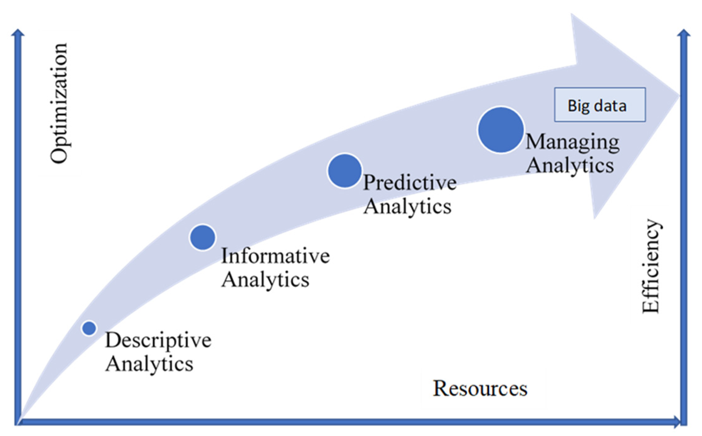
1.1. Data-Driven Approach to SC Management

Logistics scenario analysis can be used to support strategic SC (Supply Chain) management [1]. Scenarios provide industrial situations and plans for a year ahead, at least. Tactical level management adjusts these plans for the reality of procurement resources for few months’ operations. [2]. Operational management most often utilizes GIS (Geographic Information System) and routing for SC scheduling, in practice [3,4,5]. In wood SCs (WSCs) of forest industry, work schedules are prepared by contractors for a few weeks ahead, which are always based on the industry’s tactical plan available to contractors from common information systems. In order to solve a strategic scenario with information systems by data-driven DSSs (Decision Support Systems), the future wood demands of production factories must be known as accurately as possible [6] so that geographically decentralized wood procurement can be planned optimally. Most commonly, optimality has meant cost-effective regional WSCs from forests to factories [7,8]. Currently, the optimum wood procurement of carbon-neutral industry minimizes not only procurement costs, as the economic aspect, but also reduces environmental CO2 (carbon dioxide) costs [9,10]. This approach is typical of a sustainable and responsible forest industry.
Long-distance transportation is economically and environmentally the most challenging procurement operation because of remarkable fossil fuel consumption [11,12,13]. It is also the most complex operation, because many different wood assortments, roadside inventories, buffer terminals, and different transport modes form a large number of logistics combinations [14]. Therefore, synchromodal logistics systems cannot yet be integrated with strategic management systems [6]. In fact, automatization with data-driven decision support systems (DDDSSs) is ongoing in Finland for solving the operational-level routing problems of timber trucks, where transport can be coordinated on a batch-by-batch basis under cost-, emission-, and service objectives [4,5]. However, without functioning strategic coordination, no additional costs or carbon emissions can be avoided at the operational level [15,16,17]. Therefore, WSCs must be solved beforehand at the strategic level using such a DDDSS, which provides optimal SCs for synchromodal logistics planning [18,19,20].
Database management systems and cloud services seem to offer data-driven computing facilities for transportation management in WSC coordination [21]. According to the results of [22,23], cloud services facilitate SC coordination and system integration. In this respect, studies have also shown that industry can play important roles in fostering DDDSSs by encouraging SC companies to implement collaboration systems [24,25]. Additional development targets could be the standardization and the automation of information systems for more structured collaboration between companies. Then, the integration of technologies can change the strategic WSC management (WSCM), acting as enablers of a more effective adjustment to different local logistics situations [26]. Furthermore, authors have also mentioned that positive synergies exist between these two approaches, providing great impact on industrial performance [27].

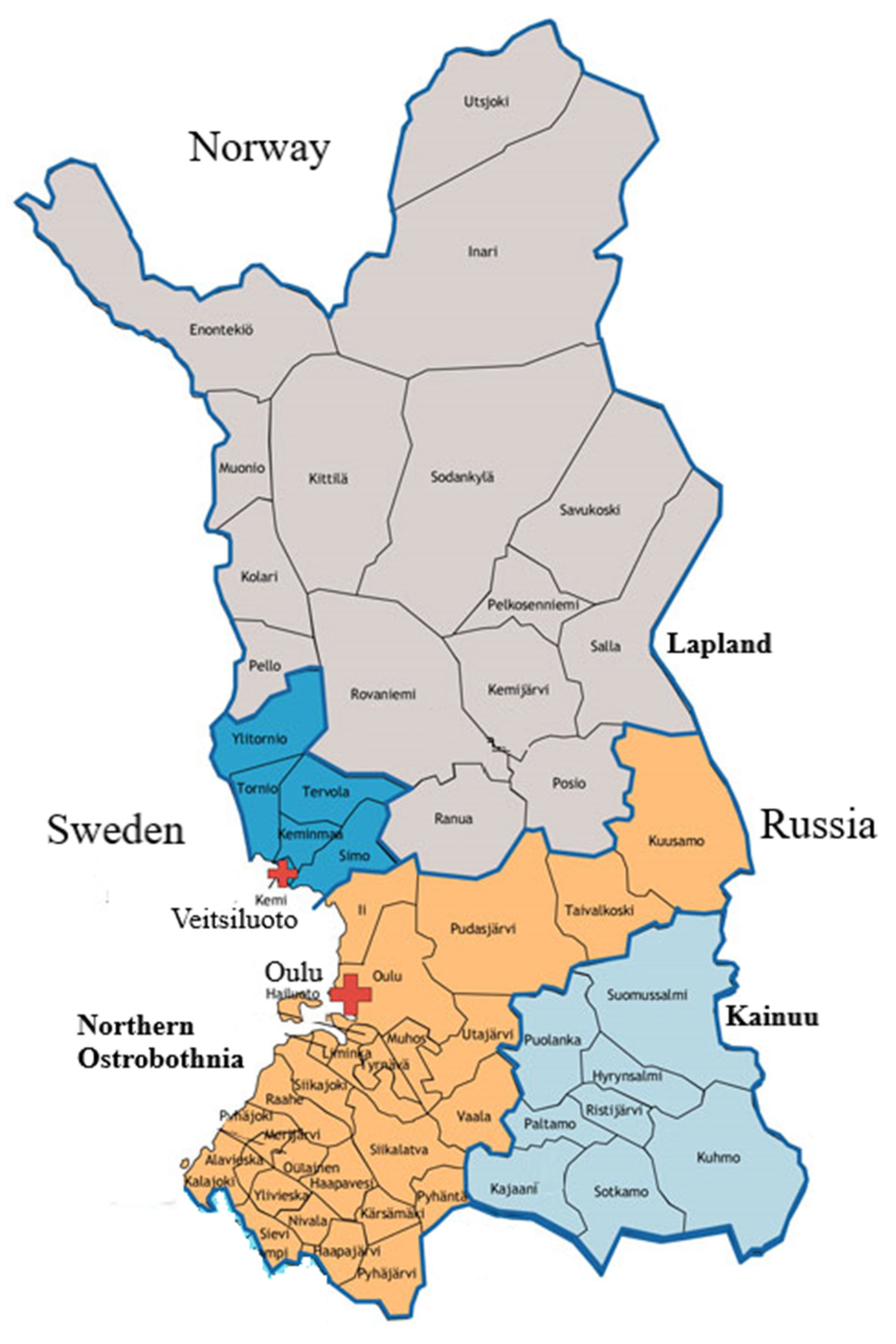
1.2. Northern Finland as a Carbon-Neutral Wood Procurement Area

The forestry of three provinces is considered in this study, all in Northern Finland: Lapland, Northern Ostrobothnia, and Kainuu (Figure 1). The province of Lapland has the largest positive difference between the country’s sustainable and actual wood harvesting amounts. The annual wood harvesting amount in Lapland’s forests in 2018 was 4.51 million m3 as solid cubic meters [28]. According to the 11th National Forest Inventory (NFI 11), the largest calculated sustainable wood harvesting accumulation estimate for 2015–2024 is 7.24 million m3 per year, of which logs amount to 1.97 million m3, pulpwood 4.15 million m3, and large-sized energy wood 1.12 million m3. In 2018, Scotch pine (Pinus sylvestris) logs accounted for 87% of the total amount of logs felled, and Scotch pine pulpwood for 73% of the felled pulpwood (Table 1).
In the province of Kainuu (Figure 1), the relative difference between the largest sustainable and realized wood harvesting is smaller than in the provinces of Lapland and Northern Ostrobothnia, because forests are used more efficiently for industrial production. The annual amount of wood harvesting in Kainuu was 3.66 million m3 in 2018 [28], while the largest sustainable harvest accumulation amount for roundwood (2015–2024) is 5.13 million m3 per year (NFI 11). Pine logs accounted for 75% of the harvested logs and pine pulpwood for 63% of the total harvested pulpwood.
The growth and thus wood production capacity of forests in Northern Finland is lower than in the south, which means that wood procurement areas of production factories are geographically wider compared to procurement areas at factories of similar size in Southern Finland. On the other hand, in the future, the largest increase in growth will occur in forests of Northern Finland because of climate warming [29]. Currently, larger procurement area challenges the profitability of wood procurement, as transport costs also increase as the result of long delivery distance. Due to the large share of ton kilometer (tkm) transported, road transport causes the largest operation expenses and fossil fuel consumption in wood procurement [13,30]. In Finland, long-distance transport can account for a third of average WSC costs, and even more in northern parts of country [31]. On northern roads, poor winter maintenance and road use restrictions, especially for the lowest road categories, also create additional challenges to transport logistics [32,33].
There are also challenges in railway transport in Northern Finland. The efficient utilization of railway transport requires large transport capacity [34]. An aim of the Finnish Transport Infrastructure Agency is to maintain and develop wood loading sites of railway stations where it is possible to load 24 wagons at a time for full-sized trains on one track [35]. Therefore, the number of loading terminals and stations on the rail network has decreased throughout the country. At the time of this research, the loading sites of Lapland were located at Patokangas (Kemijärvi), Kolari, Pello, and Rovaniemi; in Northern Ostrobothnia at Haapajärvi, Nivala, Oulainen, Ylivieska, and Ykspihlaja (Kokkola); in Kainuu at Arola (Kuhmo), Hyrynsalmi, Kontiomäki (Paltamo), Vuokatti (Sotkamo), and Ämmänsaari (Suomussalmi). In this logistics situation, changes in the multimodal transport network require careful strategic planning and collaboration between several forest industry corporations for joint transport in order to be profitable. Otherwise, the limited flexibility and wagon capacity of the VR Group, a government-owned railway company, would lead to increase costs and to road transport that is environmentally less efficient, even if it was conducted by larger and heavier vehicle combinations (LHVs).

1.3. Strategic WSCM

In addition to sustainable wood harvesting possibilities, planning at the strategic level of a wood procurement organization focuses on, among other things, the suppliers’ regional collaboration capabilities in the WSC. The geographical boundaries of the procurement regions often follow the natural boundaries of wood flows on transport routes consisting of several municipalities. The procurement region mainly occupies peripheral areas due to the decentralized demand and supply situation, which may change significantly as factory demands for the regions’ wood assortments change. In this respect, the wood procurement strategy may vary across different procurement regions in terms of delivery, purchase and sale, type of forest stand, wood pricing, and the competitive situation between modes of transport, when the region’s market share of the timber trade is adjusted to market situation.
The strategic wood procurement plan (wood flow balance) is based on available regional wood resource inventories and factory wood demand, which are usually determined for 1–5 years ahead on the basis of production plans and product demand forecasts [2,7,36,37]. To support long-term decision making, the wood flow balance can be analyzed using scenario models, such as the authors of [38] conducted when the sudden rise in Russian export tariffs caused a collapse in timber imports to Finland. Often scenarios have been prepared for the product market’s cyclical changes with the help of short- and long-term market forecasts for identifying and minimizing WSC costs, which are balancing risks in the forest industry [39,40,41].
A wood procurement scenario includes various wood sources, such as purchases from private forest owners, procurement from the corporations’ own forests, purchase and sale delivery transactions, exchanges between other companies, and wood import (Figure 2). In the modeling of a long-term wood procurement problem (logistics scenario), wood sources (supply points) are directed to delivery destinations (terminals, factories). Supply points are usually described by the forests’ wood assortment distribution, which is partly controlled by public data about the region-specific tree species distributions. This forestry data can only be managed to a limited extent in connection with purchases. Therefore, both the open public forest resource data and historic enterprise resource planning (ERP) data on the realization of the previous years’ wood procurement must be used to predict distributions of tree species and wood assortments in wood flow modeling.
In reality, wood procurement is seldom optimal because strategic planning is indicative. When the authors of [38] investigated the optimal strategic decision-making alternatives of wood procurement in changing “major” wood procurement situations caused by Russia, they found that, even in situations where the first “global” solutions to the problem were found, additional wood flow analysis (additional scenario and/or sensitivity analyses) can lead to cost savings of up to 10% as a combination of different acceptable development alternatives. This was also reported by the authors of [3], who conducted various sensitivity analyses on the Swedish Södra Cell AB. On the other hand, wood procurement is also affected by “minor” seasonal fluctuations, which are challenging to strategic WSCM and reflected at the level of operations and wood inventories.
Nature itself produces most “minor” seasonal fluctuations in operative wood procurement, especially during spring and autumn seasons [42]. In addition, the rules of the forest pest control act prohibit the storage of wood over midsummer without special protection measures [43]. Further, due to freshness requirements, logs and spruce pulpwood can be stored at roadside landings for only a few weeks during the summer season. The unevenness of wood procurement caused by seasonal fluctuations also causes an increase in wood procurement costs throughout strict WSC schedules, as the wood order of factories must be satisfied each day. In this respect, the additional costs caused by seasonality are due to overcapacity of harvesters, forwarders and wood transport fleets, road repair and maintenance costs, storage area costs, storage handling costs, additional transportation, interest on capital tied up in inventory, and from value decreases during seasonal storage [44].
In practice, wood procurement and WSC companies have operative routines for management of the “minor” seasonal variations in local municipalities. However, data-driven routines have seldom been used to adjust strategic and tactical plans. It would be interesting to test them (i.e., information flow) by DDDSSs under the changing “major” wood procurement circumstances. It seems that data-driven scenario models, analysis, and decision making would be useful for more adaptive systems, which can be used to optimize and find out more accurate “global” optimum solutions to local dynamic situations [15,45,46]. Potentially, results of the long-term (yearly based) strategic plan would also provide, as a byproduct, a more accurate wood procurement budget (financial flow), which can be further divided into a monthly, weekly, or even daily target.

1.4. Research Problem and Aims of Study

The changes in existing production facilities and the new investments planned in the forest industry will affect WSCs differently throughout Northern Finland. At the same time, it is important to take into consideration the wood resource possibilities of local regions, which also affect the wood procurement logistics. In addition, there are old factories inside the area, such as a sawmill in Kemi, which operate under profitability challenges. Therefore, scenario analysis is needed to support the WSCM of forest industry corporations, so that WSCs can be optimally adjusted to the wood demand of production facilities and guarantee carbon-neutral wood procurement.
The main optimization objective was the minimum total costs of wood procurement logistics. Environmental CO2 emission costs of forestry machinery and trucks were also included, as cost parameters, in the model. It was hypothesized that, with data-driven wood flow modeling and applied DDDSS, it is possible to integrate information systems with WSCM and select the most cost-efficient WSCs at the municipality level, thus optimizing logistics scenarios of forest industry corporations. Considering the research target, the authors address the following research questions:
(1)
How do long-distance transportation modes impact WSC practices?
(2)
How do market situations of wood resources impact WSC practices?
(3)
What implications does the integration of data-driven applications in WSCM have on strategies?

2. Materials and Methods

2.1. Database

At the time of research, three forest industry corporations operated on geographical area that was limited to Northern Finland—the provinces of Lapland, Kainuu, and Northern Ostrobothnia (Figure 1). In this experimental study, previous study data were used according to [38], which were updated from 2000 to 2019. The data was stored in Access databases and transformed automatically during the optimization [47]. In addition, the databases contained municipality-specific forest wood resources, which were updated according to the NFI 11. Maximum wood procurement amounts (m3) were based on factory environmental permits, which were regulated by environmental ministry and copied from the internet. These amounts were targeted to municipalities as minimum procurement values according to wood purchase market information published in the literature [48]. The cost values used by the authors of [38] were also updated during the data-driven process. This process used forestry machinery and truck cost indexes [49]. In the case of the absence of cost information, annual averaged wood procurement information and costs were used according to [31].
In the Access databases, wood assortments used as raw material were combined into further wood assortment entities: large-diameter pine logs, large-diameter spruce logs, pulpwood, spruce pulpwood (fiber), birch pulpwood, and wood chips. The limits of monthly wood harvesting amount per wood assortment were obtained by trial iterations, which satisfied the wood demands of factories and purchase amounts for the logistics experiment and optimal scenarios. These municipality-specific amounts were recorded as monthly data. The cubic-based wood harvesting costs of municipalities were collected from wood harvesting data of a previous study [38]. The data-driven system updated and calculated model cost data and added the environmental cost of fossil fuel consumption of forest machines and trucks based on an emission allowance price of 35€ × t−1CO2 [46]. CO2 emissions were 4.6 g × m−3 for wood harvesting and 62 g × m−3km for road transport operations [30,50]. The emission cost was 0.34€ × m−3 for an average transport distance of 156 km [12,31].
The system calculates long-distance transport costs as kilometer-based values using distances between supply and delivery points in cost models (Table 2). Here, the municipality-specific average kilometer values of [38] were used, but they can also be calculated for municipality using actual forest stand information. Optimization solves the operation amounts of WSCs, which are between set minimum and maximum operation limits, and they satisfy the wood orders of the production factories. Wood orders were calculated from public information about annual environmental permits, from the internet, and the amounts were divided evenly for months of the year. Limits of wood orders of external sawmills owned by other companies were calculated the same way, using public information. Purchases made as delivery transactions were modeled to suppliers based on the gate price of the factory, which was recorded as a cost parameter of the model. These data were also derived from public information. Gate prices are average values, which may slightly differ from real values because observations were only checked from ten factories. The model also took into account the internal sales of wood chips generated as a byproduct of sawmills and as the raw material of the pulp mills.

2.2. Data-Driven Wood Flow Optimization

The amount of information has been constantly growing in wood procurement logistics. Therefore, data for the WSC model is reasonably easy to collect automatically from big data [26,51]. To update the data-driven model, data analytics (Figure 3) were used as a support. In work for analytic tools of DDDSSs, the DLP (Dynamic Linear Programming) method is the guiding approach, which has been applied for decades in wood procurement logistics and WSCM. However, only with system automatization of data-driven modeling can the efficiency of DLP comes into use in practice [52]. This means that, with the support of automatic data mining, the general wood flow model could be customized for each customer’s logistics situation and be optimized quickly and effortlessly in servers of the service organization using information from the customer database and open public data [46].
The data-driven process aggregates local operation values for strategic management purposes. Therefore, a data-driven approach has a positive effect on the coordination of SC capabilities, which are significantly related to financial performance [17]. The data for this study were processed into a DLP model and were analyzed using LP theory. Generalization and averages used in the optimization model did not violate LP assumptions. According to [53], the linear assumptions and requirements of the model are (1) the assumption of proportionality, which means that the effect of each variable on both the objective function value and the constraints is directly proportional to the value of that variable; (2) the assumption of additivity, meaning that all variables in both the objective function and the constraints must be independent of each other to form a cumulative total effect; (3) the assumption of certainty, which assumes that the parameters are known with certainty (determinism). Uncertainty in the model could be considered indirectly using sensitivity analysis in the interpretation of the optimal solution. Some sophisticated techniques embed uncertainty elements into the LP system before optimization [20], which are not necessary for the solution of this logistics problem.

2.3. Scenario and Sensitivity Analyses

In addition to the sensitivity analysis methods typical for LP, scenario analysis is useful in the strategic planning of logistics management [1]. By changing the values of constraints of the wood flow model, the selected scenarios were used to model the changing logistics situations of the WSCs. The results were illustrated by DDDSS on maps of the wood procurement area with the support of wood flow curves. As the first step in DDDSS’s developing process, the optimal baseline scenario had to be built using the ordinary sensitivity analysis tools of LP. This scenario was as near as possible to the suboptimal WSC logistics of real wood procurement experiments.
In theory, the sensitivity the analysis of an LP solution to an optimization problem is always connected to the corner points of the solution area formed by the objective function and the constraints equations. The popular algebraic solution algorithm uses the simplex method, which traverses only a part of the corner points, proceeding to the next corner point, if the objective function becomes higher (or lower) in value, eventually reaching the optimum [53,54]. In this context, the DDDSS provided valuable information about the DLP solution (maps). Through sensitivity analysis, this made it possible to select input values from the database for logistics scenario analysis, within which the optimal solution remained acceptable. For comparison, each variable in the model and its solution has an “increased/reduced cost”. The “increased cost” (minimization problem) tells how much the total cost value of the objective function deteriorates if the value of a decision variable that is not in the optimum position is increased by one unit (m3). If the “increased cost” of the variable is zero, the variable is included in the optimal solution and is an inactive constraint. The “increased cost” of a variable was interpreted as a value that indicated how much that variable could be evolved, e.g., by reducing transport costs or purchase price to improve the optimal logistics solution.
The “shadow price” (dual price) indicated the coefficient by which the value of the objective function decreased (minimization problem) if the resource requirement of the constraint function was increased by one unit. The “shadow price” is also called the “dual price” because the value is obtained from the dual formulation of the model [53]. For example, if the total cost value of the objective function were in euros (€) and the values of the wood resource constraints were in solid cubic meters (m3), then the unit of the “shadow price” would be € m−3. In the wood flow model, for example, the “shadow price” of an active constraint could indicate that if there were one less solid cubic meter of wood resources to be transported, the total costs of WSCs would be reduced by the “shadow price”. The DDDSS software allows the addition and reduction of resources (available forest wood and procurement capacities), which allows us to see the amounts between which the “shadow price” does not change, although the optimal logistics solution may change.

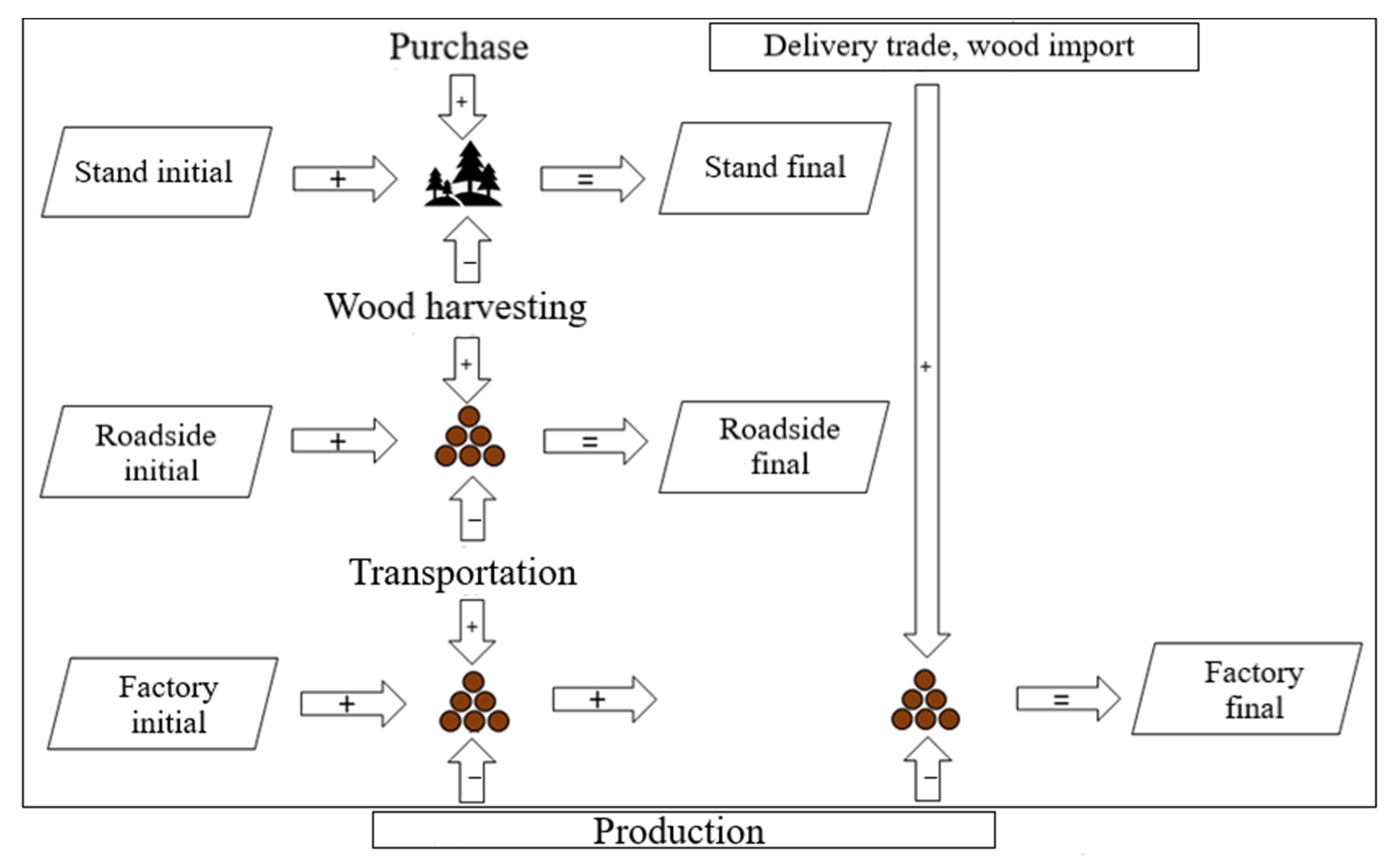
2.4. Wood Flow Model and Strategic Scenarios of Forest Industry

The wood flow model by [38] was utilized as the framework, in which one-year was divided into one-month periods. The data-driven DLP model was developed from this general model using the software DDDSS. WSCs to factories was optimized as cost-efficiently as possible by minimizing total costs. The objective function was formulated with the activities of purchasing and wood harvesting, road transport to production factories and railway stations, railway transport to factories, as well as with roadside, terminal, railway, and factory inventories (Model 1). Time-related continuation of WSC operations required the dynamism of the wood flow model [2,55]. Therefore, the WSC was formulated with time-varying efficiency parameters of capital cost, operation cost, and environmental emission cost, which affected wood flow from a municipality. The synchronizing of multimodal, long-distance transportation was implemented by the constraints. Simultaneously, roadside buffer inventories were set to meet the factory monthly wood orders at the beginning and end of the planning period. Similarly, the amounts of terminal and factory inventories were determined to correspond to their target inventory quantities (buffer amounts) at the beginning and end of the planning period (year).
Min Z [ i = 1 I j = 1 J t = 1 T ( ( c p i j t + c l i j t + c a l i j t L i j t × ( 1 + ( p / 12 ) ) t ) + i = 1 I j = 1 J k = 1 K l = 1 L t = 1 T ( ( c y i j k l t + c a y i j k l t ) Y i j k l t × ( 1 + ( p / 12 ) ) t ) + i = 1 I j = 1 J k = 1 K l = 1 L t = 1 T ( ( c y h i j k l t + c a y h i j k l t ) Y H i j k l t × ( 1 + ( p / 12 ) ) t ) + i = 1 I j = 1 J t = 1 T ( c x i j t X i j t × ( 1 + ( p / 12 ) ) t ) + i = 1 I j = 1 J l = 1 L t = 1 T ( c r i j l t R i j l t × ( 1 + ( p / 12 ) ) t ) + i = 1 I k = 1 K t = 1 T ( c m i k t M i k t × ( 1 + ( p / 12 ) ) t ) ]
The factory wood order, i.e., Equation (2a,b), was determined on a factory-by-factory basis for each period. Operations were limited by the continuity of activities, i.e., the dynamism of the wood flow models also required the use of dynamic equations as Constraint (3a–c). The wood flows were assumed to operate uniformly without internal interferences, but quantitative restrictions on wood harvesting amounts (Equation (4a,b)) were used, which could be procured from the municipality during a certain period or purchased by delivery purchases. Quantitative constraints considered how much wood could be transported from the municipality’s area or railway station’s inventory, even more so if there was harvested wood during the period (Equation (5a–d)). For roadsides, railways, and factories, initial and final inventories were determined for the first and last period (Equation (6a,b)) (Equation (7a,b)) (Equation (8a–d)). The variables of the DLP model also had constraints on non-negativity (9).
Wood orders of the factories are:
Mikt−1 + Yijklt + YHijklt ≥ Dminikt
Mikt−1 + Yijklt + YHijklt ≤ Dmaxikt
The dynamic equation of roadside inventory is:
Xijt−1 + Lijt − Yijklt = Xijt
The dynamic equation of railway station inventory is:
Rijlt−1 + Yijklt − YHijklt = Rijlt
The dynamic equation of factory inventory is:
Mikt−1 + Yijklt + YHijklt − Dikt = Mikt
Wood harvesting constraints are:
Lijt ≥ Lminijt
Lijt ≤ Lmaxijt
Road transport constraints are:
Yijklt ≥ Yminijt
Yijklt ≤ Ymaxijt
Railway transport constraints are:
YHijklt ≥ YHminijklt
YHijklt ≤ YHmaxijklt
Roadside inventory constraints are:
Xijt = 0 = XIij
Xijt = 12 = XBij
Railway station inventory constraints are:
Rijlt = 0 = RIil
Rijlt = 12 = RBil
Factory inventory constraints are:
Mikt ≥ Mminikt
Mikt ≤ Mmaxikt
Mikt = 0 = MIik
Mikt = 12 = MBik
Non-negativity constraints are:
Y i j k l t , Y H i j k l t , L i j t , X i j t , R i j l t , M i k t = 0
This study applied an experimental approach to answer the research questions. After the optimization of logistics scenarios, the scenario analysis and sensitivity analysis were applied for quality evaluation of the model. This was first conducted by comparing the optimized results of the baseline scenario to the initial experiment. Then, the results obtained from the scenarios were compared with the baseline scenario, to identify the most sensitive municipalities as targets of different wood orders of forest industry integrates. This experimental analysis reported WSCs by considering efficiency of long-distance transportation modes and local market shares. The propositions and discussion of the integration of data-driven application into WSCM are presented in Section 4, which also presents research directions for future studies, and Section 5 concludes the study.
The logistics scenarios were formed as experiments based on objectives and predictions set at the strategic level of the forest industry. It was assumed that a future state of investment will develop from the optimized supply state (baseline scenario). Therefore, the optimization model was changed by the data of the scenarios, and the optimum solutions of the scenarios were compared to the baseline scenario, and to the “global” optimum solution of the wood flow model, which represented the WSCs’ amounts for a procurement year of the forest industry.
(1)
“Baseline” Scenario
The optimal wood order of sawmills, 422,966 m3, was applied as the experiment. The wood flows were optimized according to the presented model. The two scenarios for new supply situations were:
(2)
“The decreasing sawmill wood demand” Scenario 1
The wood order of sawmills was reduced to 400 000 m3 per year in integrate A. The demand for pulpwood was increased 1.35 times in integrate B, corresponding to 2.7 million m3 of annual wood order. As the supply amounts of pulpwood increase, so do the quantities of logs. In order to maintain a useable distribution of wood assortments and “global optimum solution”, the wood orders of certain private sawmills were increased in the model by 10%.
(3)
“The increasing sawmill wood demand” Scenario 2
The wood order of sawmills increased to 480,000 m3 per year in integrate A. Correspondingly, the wood order of private sawmills decreased in the model, and the demand for pulpwood increased 1.35 times in integrate B, corresponding to 2.7 million m3 of annual wood order.

3. Results

3.1. Logistics Optimum of Baseline Scenario

The optimized baseline scenario was used in comparisons with other scenarios because the actual experiment for wood procurement of the forest industry did not operate optimally. Based on the updated cost data and modified operation data, the model was customized by a data-driven process and solved by the DDDSS that produced the “global optimal solution” to the WSC problem. Table 2 and Table 3 show the differences in transport amounts per wood assortment between optimized and actual experiments. In the validity tests, the optimal solution of the baseline scenario was lost when the model’s initial wood inventories were reduced towards the initial experiment’s values, leading to a situation where pulpwood was not sufficiently available to the forest industry. Total costs of wood procurement logistics according to the baseline scenario were 4.9% lower than the costs of the initial experiment. Long-distance transport costs, on the other hand, increased by 23.3% (Table 3). In solving the optimization model, cost changes mainly resulted from increasing the corporations’ own wood procurement and decreasing delivery purchase amounts. Cost changes were also affected by the environmental costs of CO2 emissions, which were included in the experiments but not used in practice. Truck CO2 emissions (49.6 g × tkm−1, 62 g × m3 km−1 by using fossil fuel) affected the cost parameter of long-distance transport (+5.5% to road transport costs, +0.7% to total transport costs).

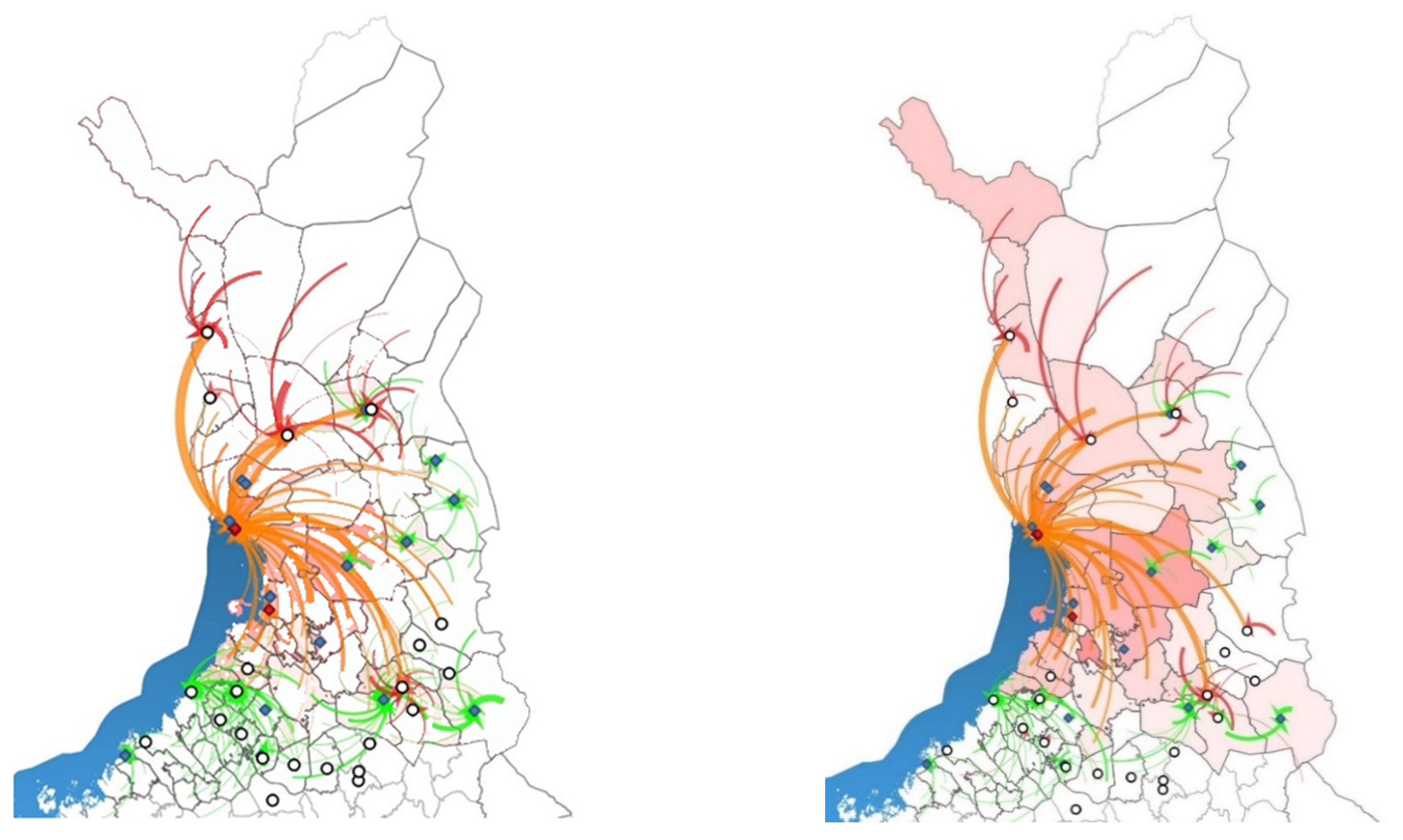
3.2. Comparison of Pine Log Wood Flows between Logistics Baseline Scenario and Initial Experiment

The pine log flow amount of the corporations’ own WSCs increased by 3.6% in the baseline scenario compared to the initial experiment. Figure 4 shows municipality-specific wood flows for pine logs, using a map to improve the visibility of the results. Accordingly, the delivery amounts to private sawmills decreased slightly. Changes in the pine log flow were observed in the peripheral municipalities of wood procurement area, especially in Eastern and Western Lapland, Kainuu, and in the municipalities south of Oulu.
The baseline scenario’s average WSC costs of the pine logs, excluding delivery purchases, decreased by 7% compared to the initial experiment’s WSC costs. Within the limits set by the optimization model, the average long-distance transport cost of pine logs was 7 € m−3, and the cost of direct road transport to sawmills was 8 € m−3. Figure 5 shows that the amount of delivery purchases of pine logs decreased, while direct road transport increased remarkably (52%). In the baseline scenario, a total of 222,300 m3 pine logs were supplied by direct road transport to sawmills from a total of 26 municipalities (Figure 4 and Figure 5). The corresponding amount of railway transport decreased 5%. Of the municipalities that used road transport to sawmills, the gate price of pine logs was 69 € m−3. For municipalities using railway transport, the price was 65 € m−3.
In contrast to the WSCs of pine logs in the experiment, they were not supplied by direct road transport from Kainuu province to the sawmills of the experiment in the baseline scenario (Figure 1 and Figure 4). In the experimental wood flow, pine logs were supplied to the Kajaani sawmill (Pölkky Oy) from Kuhmo, Kärsämäki, Suomussalmi, Vaala, and Siikalatva. In terms of WSC amount (m3), the most significant difference was in the municipality of Siikalatva, from where the pine log flow turned towards the sawmills of the experiment instead of the Kajaani sawmill, although the transport cost was almost double. Based on the “reduced costs” of the DLP, transporting from Siikalatva to the Kajaani sawmill increases the value of the objective function by 2.0–3.0 € m−3. For the Kajaani sawmill, pine logs were directed from the southwest municipalities of Kainuu: Haapajärvi, Kajaani, Paltamo, Pyhäjärvi, Pyhäntä, and Sotkamo. Unlike in the experimental wood flow, pine logs were directed to Ämmänsaari railway station only from Suomussalmi municipality. In the experimental wood flow, pine logs were also transported from Hyrynsalmi to the same station. When experimental wood flow supplied pine logs from Vaala to Kontiomäki station, optimization supplied all pine logs from Vaala directly by road transport to the sawmills of the experiment. Based on the “reduced costs” of the LP, transporting from Vaala to the Kajaani sawmill would increase the value of the objective function by 2.11–3.11 € m−3.
In the baseline scenario, pine logs of Eastern Lapland were sent to sawmills by rail from Patokangas, Pello, Kolari, Rovaniemi, Vuokatti, Kontiomäki, and Ämmänsaari railway stations, with transport costs of 4.4 € m−3 on average. Pine logs were supplied to Patokangas station from the region of four municipalities: Kemijärvi, Pelkosenniemi, Salla, and Savukoski (Figure 1 and Figure 4). The highest costs arose from Savukoski, of which the road transport cost to the Patokangas station was 10 € m−3. The average road transport cost to Patokangas station was 6 € m−3, while directly to sawmill the road transport costs was 14 € m−3. From Salla, in addition to Patokangas station, pine logs were supplied to Kemijärvi sawmill (Lappi Timber Oy), Kitka sawmill (Kitkawood Oy), Kuusamo sawmill. From Posio, the pine log flow was supplied only by direct road transport to the sawmills of the experiment. From Sodankylä, all pine logs were supplied to Rovaniemi station. Pine logs of Western Lapland from the municipalities of Enontekiö, Kolari, and Muonio were supplied to Kolari station. From Kittilä, the pine log supply to Kolari station decreased considerably compared to the experimental wood flow, and the pine log flow turned exclusively to the Rovaniemi station. Unlike in the experimental wood flow, pine logs harvested from Rovaniemi were sent by direct road transport to the sawmill.

3.3. Comparison of Pulpwood Flows between Logistics Baseline Scenario and Initial Experiment

In the pulpwood flow to integrate A, significant differences between the baseline scenario and the experiment were observed in the delivery purchase amounts (Figure 6). The share of these amounts increased in the baseline scenario. On the other hand, the delivery purchase amount decreased remarkably for integrate B. Therefore, the costs of the total wood procurement logistics decreased by 2.7%. In the baseline scenario, long-distance transport amounts increased by 9.6% compared to the experimental wood flow (Table 2 and Table 3). In particular, road transport amounts increased by 27.8%, raising direct transport costs by 35.3%. Unit road transport cost of the baseline scenario was 7.5 € m−3.
Significant changes were observed in WSC amounts of procurement regions, because the cross-transportation observed in the experimental flow in the regions ceased (Figure 7). In Kainuu, differences arose in the diversion of wood to different railway stations. In Western and Eastern Lapland, the clearest difference was wood supply from the municipality of Kittilä to Rovaniemi railway station. Further, in Southern Lapland, changes were observed in wood flows in the municipalities of Ranua and Posio, using direct road transport to the integrate A in the baseline scenario. In addition, wood was still delivered to Metsä Group’s integrate to Kemi from the Patokangas station, and from Western Lapland.

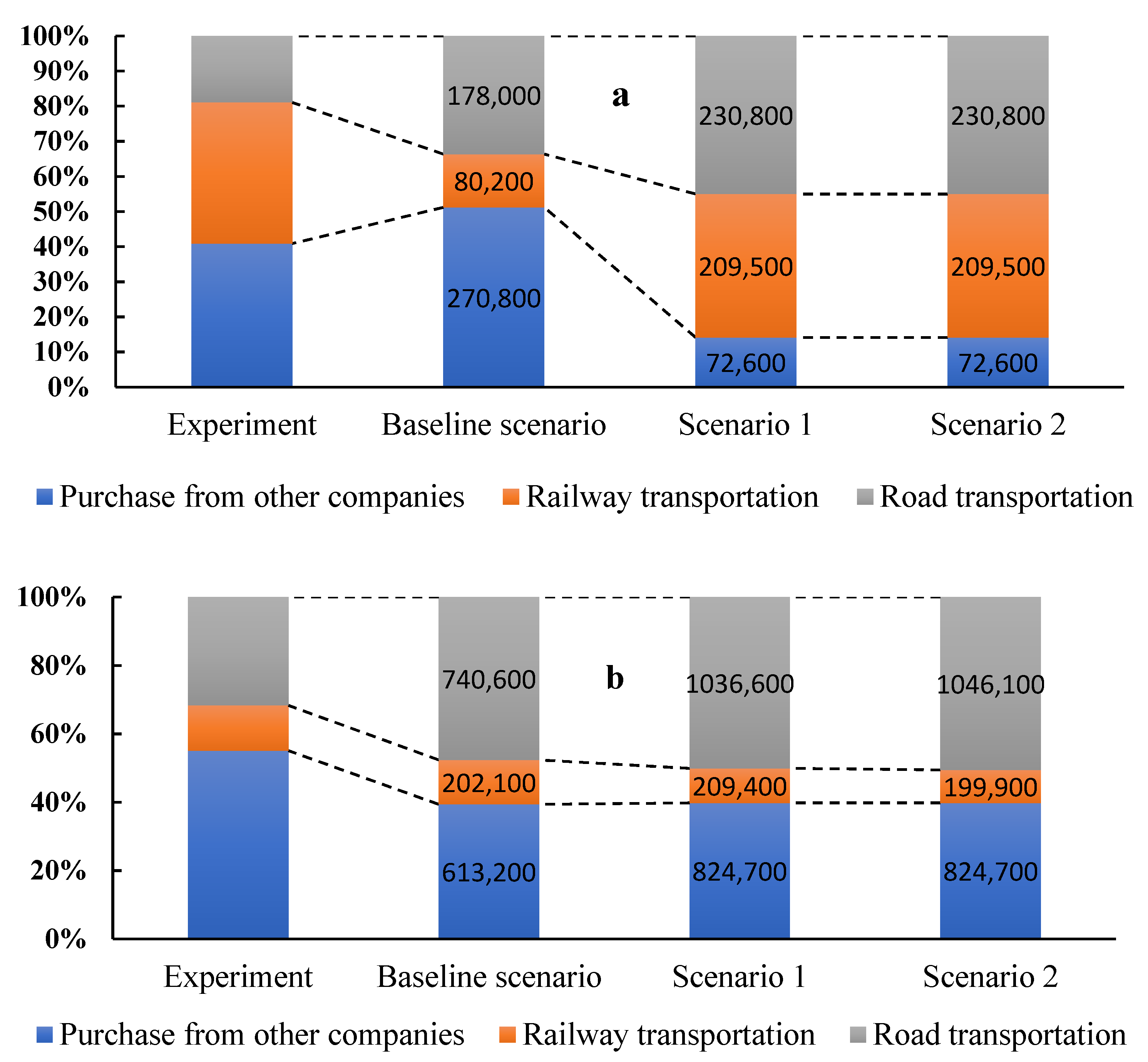
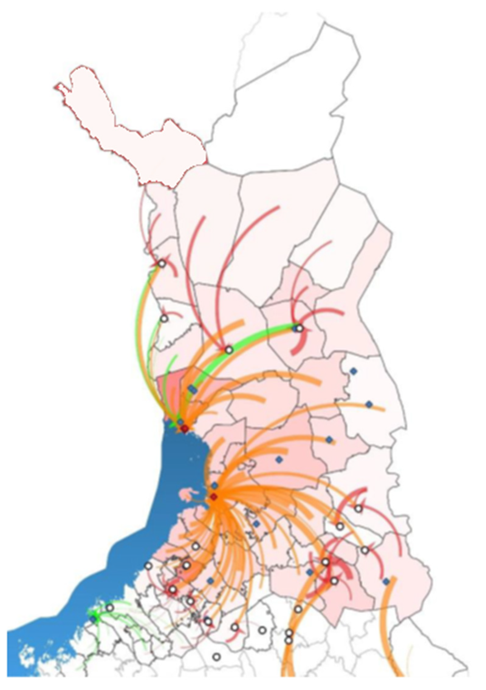
3.4. Optimum Solutions of Pine Log WSCs in Logistics Scenarios

In Scenarios 2 and 3, the results were “global” optimal solutions, with values of 157,030,119 € and 161,397,370 € as the minimum total costs, respectively. In Scenario 1, the long-distance transport amount of pine logs was 32,000 m3 lower than the amount of baseline scenario; in Scenario 2, the long-distance transport amount was 51,000 m3 higher than the baseline scenario’s transport amount.
In Scenario 1, a total of 227,100 m3 pine logs were delivered to sawmills of the experiment by direct road transport from 25 municipalities, and 62,700 m3 by railway transport from six railway stations, to which pine logs were transported from 14 municipalities (Figure 5 and Figure 8). Unit transport costs from direct road transport averaged 9.1 € m−3, road transport costs to stations averaged 5 € m−3, and railway transport cost was 4.5 € m−3. The average gate price at the sawmills was 68 € m−3, while for direct road transport it was 69 € m−3, and for railway transport 65 € m−3. The same amount of pine logs was purchased as delivery purchases as in the baseline scenario, i.e., 104,600 m3. The average cost of pine log delivery purchases was 67 € m−3, and the selling price was 70 € m−3. Only 8000 m3 more pine logs were delivered to sawmills of other companies than in the baseline scenario, which varied between 1–16%. In this respect, delivery amounts to the Kalajoki sawmill increased the most.
In Scenario 2, the long-distance transport amount increased significantly from the baseline scenario. The amount of pine log flow increased to 537,000 m3, from which 266,900 m3 were delivered to sawmills of the experiment by direct road transport, 93,800 m3 by railway transport, and 104,600 m3 by delivery purchases. In relative terms (€ m−3), transport unit costs were 44% higher, with total transport costs being 28% higher. Unit transport costs of pine logs to sawmills averaged 10.2 € m−3 for direct road transport, 5.3 € m−3 for initial road transport to railway stations, and 4.7 € m−3 for railway transport. Contrary to expectations, the average gate price decreased slightly from Scenario 1 to 67.8 € m−3. The costs were 69 € m−3 via direct road transport and 64 € m−3 via railway transport. The increase in road transport amounts of pine logs to railway stations with the initial road transport price that was cheaper apparently affected the gate price at the sawmill. In Scenario 2, the average cost of delivery purchases of pine logs was 67 € m−3, and the selling price was 69 € m−3.

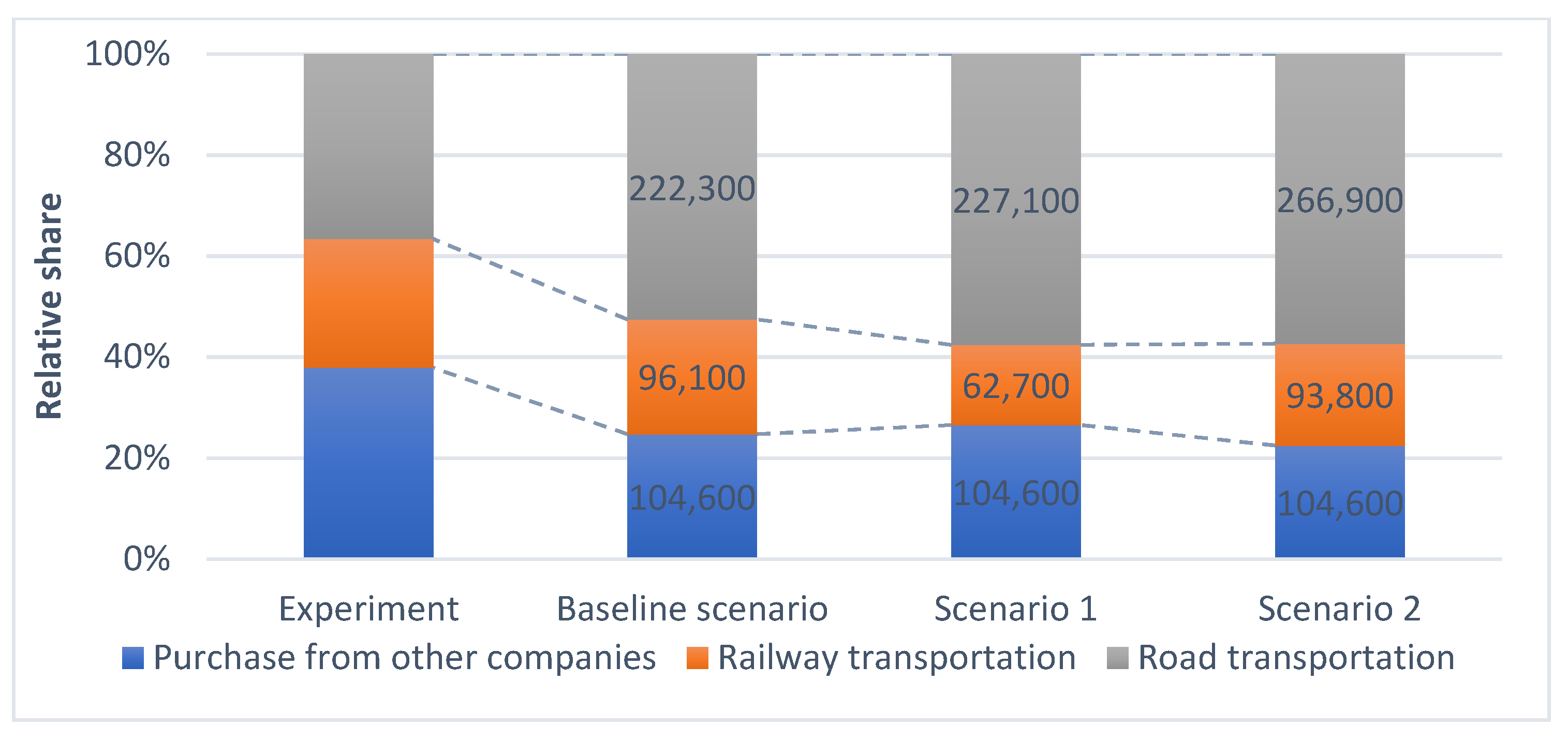
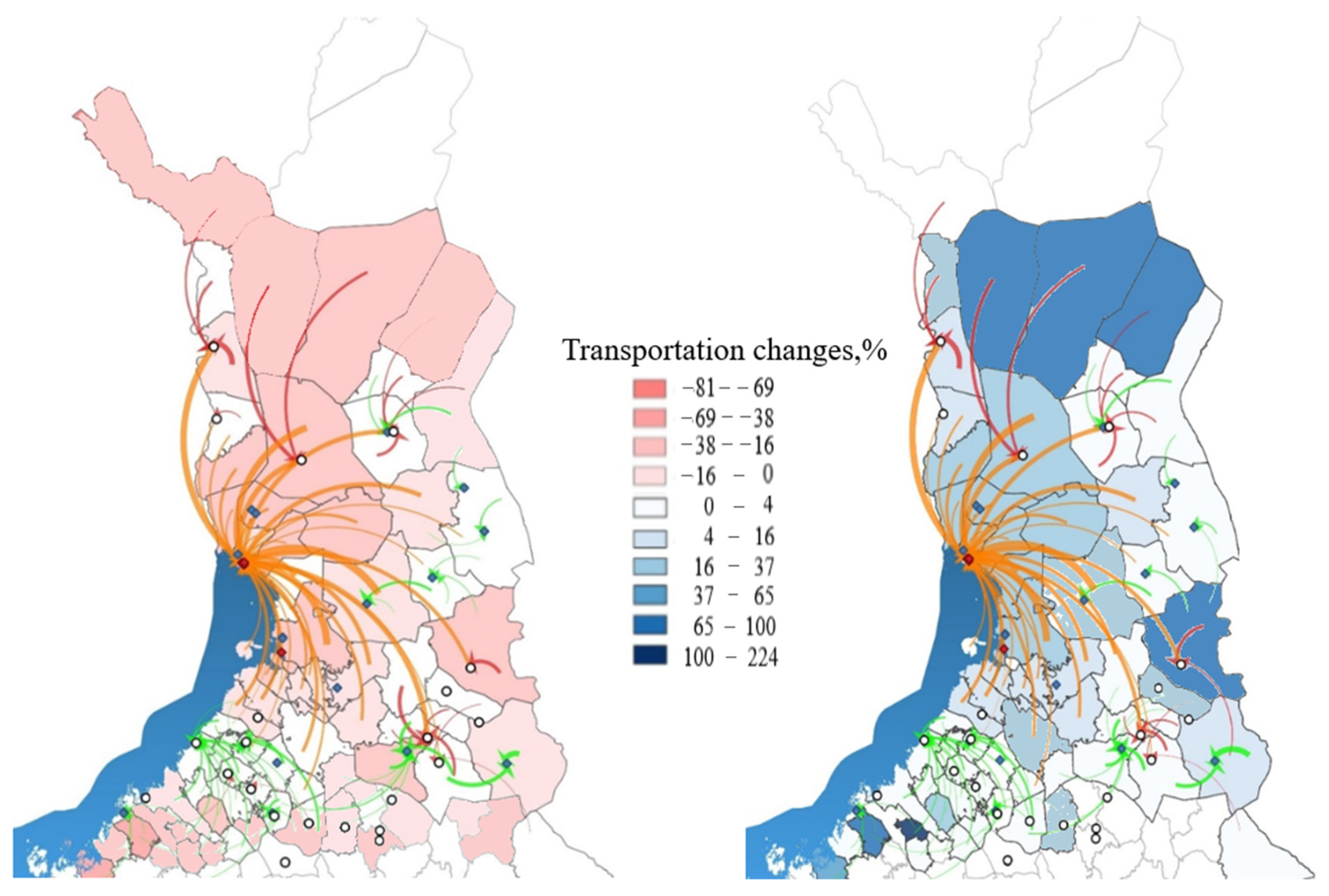
3.5. Market Shares of WSCs in Municipalities of Logistics Scenarios

The annual wood demand of pine logs increased to 480,000 m3 in Scenario 2. When comparing the results obtained from Scenario 2 to the pine log flows of the baseline scenario, the largest increases for WSCs were due to short transport distances from the vicinity to the sawmills of the experiment, mainly from the north of Oulu (Figure 1 and Figure 9). Moderate growth of market shares was observed in the provinces of Lapland, Northern Ostrobothnia, and in the municipality of Kuhmo in the province of Kainuu. Especially, in eastern parts of the provinces of Lapland and Northern Ostrobothnia, increasing market share is probably easier than in municipalities of coastal regions. In these hinterlands, pine log flows increased by 8–21%, with market shares of less than 10%, e.g., the market share in Kuusamo was only 3%.
The third but more challenging region for increasing market share of pine logs is the province of Kainuu (Figure 1 and Figure 9). Commercial collaboration with private sawmills in the region is essential; for example, the majority of pine logs were supplied to the Kuhmo sawmill, while only a third of pine logs were transported from Kuhmo to the sawmills of the experiment via the Ämmänsaari railway station. The market shares were quite good in the municipalities of Puolanka (7%) and Kuhmo (13%). Considering the market share alone, the municipalities of Suomussalmi and Hyrynsalmi could also be potential areas for additional purchases of pine logs, but the optimized WSC amounts in Scenario 2 were more than 8% lower than in the baseline scenario’s WSCs, which suggests unprofitable purchase. Furthermore, the forests’ wood resources are used efficiently in Kainuu, which highlights existing competition that also causes the small difference between the largest sustainable potential and the realized wood procurement (Table 1).
In the Haapavesi–Oulainen region of the province of Northern Ostrobothnia, a logistics border zone existed from which the pine log flow did not increase or decrease in relation to baseline scenario’s wood flow. The WSCs in the region were affected by large private sawmills, in the vicinity of which the wood procurement potential was efficiently used. In the same province, the pine log flow to the sawmills of the experiment decreased in municipalities of Kiuruvesi, Lestijärvi, Nivala, Oulainen, Pyhäntä, and Ylivieska. There were also municipalities under the same situation in the provinces of Lapland (Enontekiö, Pello, Sodankylä) and Kainuu (Hyrynsalmi, Kajaani, Paltamo, Suomussalmi).

4. Discussion

4.1. Benefits and Shortcomings of Data-Driven Wood Flow Optimization

Several authors have reported that automatized solving of decision-making problems could open up information systems for more convenient optimization and decision support in SCM [19,26,51]. We demonstrated this suggestion successfully in practice using the DDDSS in WSCM. Authors have also reported that digitalization and the big data (ERP systems and open public information) are important elements of the logistics management in large forest industry corporations [8,56]. In this respect, this study shows the usefulness of data-driven modeling, automatic data analytics, and data mining. With these elements, it is possible to combine information for wood flow optimization from the forest industry corporations’ databases and open public information sources. In fact, data-driven decision support has already been applied for over sixty years [52], but current effective computerized systems with automatization can provide more benefits for SCM [17,26,46]. These suggestions were confirmed in practice by integrating our data-driven application with WSCM.
The practical aim was to optimize the WSCs of an experiment in Northern Finland. Three scenarios were prepared revealing the impacts of new pulp production investment and changing wood flows of a sawmill on procurement logistics. The discussion of the results sought answers at the strategic level, although the solution would also allow reviews at the tactical level, that several studies have used, e.g., for reasons of monthly operation fluctuation [57]. The tactical considerations were omitted from this study. Instead, strategic scenarios were used. Results of scenarios are often compared directly to the initial practical experiment of SCs [1]. However, wood flows of the initial experiment were suboptimal to monthly wood harvesting, transport, and inventory amounts of WSCs. Therefore, the initial experiment could not be used in the scenario analysis. Instead, the results of the scenarios were compared with optimized wood flows corresponding to near experimental flows, i.e., the baseline scenario. These logistics scenarios were solved by imitating the automatic data-driven optimization. This optimization approach provided the benefits of more accurate information of regions for the utilization of DDDSS in WSCM.
The optimization model used has a strong theoretical basis because it has been applied successfully in several strategic studies of wood procurement logistics [3,38]. In this new version, the synchromodal long-distance transport logistics that were modeled worked reliably. Compared to the previous synchromodal models in ref. [4], synchronizing road transport, rail transport, and railway terminals were modeled as a strategic application. With automated data-driven modeling, multimodal capacity analyses were performed in addition to separate road and railway capacities [6,34]. In fact, the long-distance transport function of the model can be developed further for improving the efficiency of procurement logistics. For example, the model was based on municipality-specific averages of transport distances and costs. In areas with several small railway terminals, road transport was directed to one of them based on the shortest distance. It may be worthwhile to use road transport from a large municipality to several railway stations.
The wood flow results obtained need to be considered with the literature and in terms of larger geographical areas than municipality. In previous studies, optimization has achieved 3–4% cost savings in wood flow in the same region of Northern Finland [38]. In Northern Sweden, optimization has achieved almost similar results of 3.9–4.6% [3,36]. The total cost savings achieved in this study were 4.9% (3–7% depending on the wood assortment) supporting the previous results. As digitalization has evolved in wood procurement planning in recent decades, and, based on this technological development, it could be assumed that, currently, the wood flow is more optimal than in previous decades. However, the results obtained do not fully support this view. Therefore, real attention should be paid towards evolving the future for the automatization of data-driven modeling of wood flows. Otherwise, some benefits of SCM promised by authors of transport logistics [17,18,51] may be left unutilized in practice.
The optimization method is very sensitive regarding the model’s cost changes and buffer amount variations in wood inventory, which are possible to adjust by automatization using the constraints of inventory turnaround speeds. These changes may also change the resulting WSC solution. However, wood supply is also affected by many other strategic factors that are more challenging to automatize, such as market competition, environmental sustainability of regional wood resources, collaboration of partners, and customer relationships. These fluctuations cause demand uncertainty. Recently, new data-driven approaches have been suggested for solving uncertainty problems [20], which may be applicable, in theory, to this kind of large-scale WSC problem in the future. Fortunately, the constraints of our model were quite strict and sought above all to describe the experimental wood supply situation as accurately as possible. Consequently, despite the shortcomings, the model strives to supply the raw material as cheaply as possible to both the corporation’s own and other production factories following the logistics of raw material. Therefore, the relative costs of the initial experiment and scenario-based WSCs are plausibly comparable within the limits and generalizations made by the user in the wood flow model.
The authors of ref. [5] have shown that environmental emission limits and emission allocation schemes impact intermodal freight transportation in operative logistics problems. In fact, the issue addressed in our study focused on a strategic optimization problem. Therefore, costs were modeled using aggregated average cost parameters consisting of both the economic and emission aspects. They together caused the cost impacts to wood procurement logistics, when the logistics scenarios were solved for wood orders of factories through an intermodal transportation network as a part of the wood flows of municipalities. Forest resource regulations are national and EU issues. Therefore, we consider CO2 emissions using the EU’s emission allowance price mechanism in data-driven calculations of emission cost parameters that transfer the emission implications to the factory wood orders via wood flow allocations. Cost effects increased total costs, but we cannot yet separate emission changes in operative allocations and produce emission information for a single operation, which will be future issues for transport logistics studies.

4.2. Impacts of Intermodal Network on Transport Logistics

Scenarios show that long-distance transportation modes impact both amounts and costs of WSCs. Municipalities were identified that are “logistics water dividers” of wood flows in the peripheral areas, which are the most sensitive to changes in the transport modes of WSCs. This is important information for the enhancement of WSCM, which also supports the observations of the Finnish Forest Centre [32] on wood flows and transport amounts. Subsequently, supply regions are expanding and, especially, road transport amounts are increasing, thus transport distances will be longer. According to [58], reducing industrial production would also change the rail transport from stations in Eastern Lapland and Northern Ostrobothnia. We found by comparison that additional production investment would increase the need for railway transport from Eastern Lapland. The investment will also turn Kainuu’s wood flows from Northern Ostrobothnia towards factories of integrate B. Thus, the results obtained justify strategic suggestions of the increasing needs for investments to railway transport capacity [32]. It is good to remember that factory orders with lowest emission limits are allocated through railways, and emission-minimizing solutions often use a mix of allocation schemes in an intermodal network [5]. In this study, railway transport capacity was not increased from the actual level, and, partly for that reason, costs of transport logistics increased by 23.3%. To generalize for transport logistics in WSCM, this means that infrastructure significantly affects WSC capabilities, which also corresponds to the studies of [17,34], although these authors modeled SCs in different logistics contexts.
Transport logistics accounted for about one-fifth of total logistics costs. These results are consistent with the studies of [12,31]. As these studies state, the purchase of pine logs was much more expensive than pulpwood purchases, and transport logistics costs of pulpwood can even be a third of total costs. In our baseline scenario, the transport logistics costs of pine logs increased by 18% compared to the costs of initial experiment, which means that, in relative terms (€ m−3), growth was 5%. Road transport caused the largest expenses in transport logistics. Direct road transport from the northeast to the factories of the experiment was growing because transport through railway stations was not cost optimal. One alternative option is to make more efficient use of higher capacity road transport, the cost benefits of which are reflected from routes with longer transport distances. However, the special routes in the infrastructure of Finland are currently only allowed for LHVs. It is also important to notice in WSCM that, as the delivery purchases of pulpwood transferred from the integrate A to the integrate B, the resulting wood deficit was offset by an increase in transport amounts, especially from Northeast and Eastern Lapland. This raises the WSCM question of whether transporting pulpwood from these regions by railway transport to the integrate B would be more optimal. This is an issue for future mode shift studies that are also related to railway capacity, because, in this intermodal network, railway transport from these regions was only allowed to integrate A.

4.3. Implications of Market Shares for WSCM

It is commonly known that the profitability of sawmills is fluctuating by following market cycles, and there is also continuing concern about the adequacy of pine logs as a renewable raw material, i.e., about market shares in municipalities. When increasing the annual wood demand for pine logs to 480,000 m3 (Scenario 2), it was observed in the optimization that delivery sales amount decreased to some private sawmills located in the eastern border municipalities. The results are logical because the sawmills are located inside the new, larger wood procurement area of integrate A (Figure 1 and Figure 9). On the other hand, the delivery sales increased by 1–10% to Junnikkala’s sawmill, Taivalkoski’s sawmill, and to Kajaani’s sawmill, which are outside the procurement area.
The largest increases in WSCs were due to short transport distances in the vicinity of the sawmills of the experiment. However, it should be noted that the market share of pine logs in the region was 30–50% to both forest industry corporations, and increasing it can be challenging, because factory production shares are constant at corporations and limited by factory environmental regulations.
The strategic suggestions made by the authors of [32], that log flow would increase from the west to the east in the future, does not fully support the findings of this study. The optimization directed pine logs from Eastern Lapland to Rovaniemi railway station, or by direct road transport to the western sawmills, almost regardless of the wood order of the sawmills of the experiment. In contrast, in Kainuu, the west–east directed wood flow of pine logs of the Kuhmo sawmill depends on the wood orders of the sawmills of the experiment. Presumably, the increase in procurement amounts in Kainuu with the increasing long-distance transport via Kontiomäki railway station together could maintain sufficient market shares, because there are more available wood resources in the municipalities of Kainuu. This positive strategic information for increasing log purchasing amount in the region is also supported by the possibilities of increasing WSC amounts of pulpwood in the same regions, and the results of increase in renewable wood procurement opportunities [29,59]. However, the problem in these municipalities is long transport distances to both the sawmills and to the railway stations.
Optimization revealed that additional wood procurement should be targeted at four geographical regions in Northern Finland, which usually requires increasing market shares related to renewable wood resources in these municipalities (Figure 9). In this respect, however, environmental emission costs as a collective risk caused by increasing market share are not yet such an accurate element of the optimization model to have greatly affected the results. Therefore, as a future improvement to the model, considering the market shares’ implications with sustainable use of wood resources is necessary because increasing market shares are more challenging if renewable wood resources are already fully exploited in a municipality. It is therefore obvious that the most sensitive municipalities could be successfully identified for retaining the carbon neutrality of WSCs using more advanced DDDSS. If factory wood demand are increased in future, data-driven modeling of the objective function could check the sustainability issue and add emission costs to purchased amounts. According to the Finnish Forest Center [32], the total accumulation of wood harvesting amounts in the region is too high compared to the annual sustainable growth of forests. Therefore, the overall market situation in Northern Finland is so challenging that this optimization experiment drove down the pulp production facilities of integrate A, although data-driven market elements were not ready to be integrated into the model. This may be a reasonable strategy because other forest industry corporations will also invest in Northern Finland.

5. Conclusions

The scenario optimization by the data-driven wood flow model successfully solved the logistics changes in forest industry. The transport modes and railway terminals formed synchromodal logistics elements in the DLP model, which worked reliably in practice for WSCs. In addition to economic costs, the model also used environmental CO2 emission costs of wood harvesting and transportation. The optimization of wood procurement logistics resulted in the total cost saving of 4.9%. Consequently, automized data-driven optimization is beneficial in DSS for strategic WSCM. Based on the information of larger logistics Scenario 2, the amount of the delivery purchases to factories should, as a rule, be reduced and replaced by the corporations’ own WSCs. Further, increasing market shares was significant at four regions. However, logistics transport costs increased by 23.3%. Therefore, increasing transport amounts requires investments in national railway transport capacity, railway terminals, and/or LHVs, which are the most cost- and emission-efficient alternatives in transport logistics. The discussion also provides a practical framework for the emission allowance price compensation mechanism in forestry, when strategic decisions about additional investing or driving down of the production facilities are executed in the EU towards a carbon-neutral forest industry.

Author Contributions

Writing—review and editing T.P.; Software, L.V. All authors have read and agreed to the published version of the manuscript.

Funding

This research received no external funding.

Conflicts of Interest

The authors declare no conflict of interest.

References

  1. Rodrigues, V.S.; Pettit, S.; Harris, I.; Beresford, A.; Piecyk, M.; Yang, Z.; Ng, A. UK supply chain carbon mitigation strategies using alternative ports and multimodal freight transport operations. Transp. Res. Part E Logist. Transp. Rev. 2015, 78, 40–56. [Google Scholar] [CrossRef] [Green Version]
  2. Palander, T. Tactical Models of Wood-Procurement Teams for Geographically Decentralized Group Decision-Making. Ph.D. Thesis, University of Eastern Finland, Joensuu, Finland, 1998. [Google Scholar]
  3. Carlsson, D.; Rönnqvist, M. Supply chain Management in forestry–case studies at Södra Cell AB. Eur. J. Oper. Res. 2005, 163, 589–616. [Google Scholar] [CrossRef]
  4. Qu, W.; Rezaei, J.; Maknoon, Y.; Tavasszy, L. Hinterland freight transportation replanning model under the framework of synchromodality. Transp. Res. Part E Logist. Transp. Rev. 2019, 131, 308–328. [Google Scholar] [CrossRef]
  5. Heinold, A.; Meisel, F. Emission limits and emission allocation schemes in intermodal freight transportation. Transp. Res. Part E Logist. Transp. Rev. 2020, 141, 101963. [Google Scholar] [CrossRef]
  6. Giusti, R.; Manerba, D.; Bruno, G.; Tadei, R. Synchromodal logistics: An overview of critical success factors, enabling technologies, and open research issues. Transp. Res. Part E Logist. Transp. Rev. 2019, 129, 92–110. [Google Scholar] [CrossRef]
  7. D’Amours, S.; Rönnqvist, M.; Weintraub, A. Using Operational Research for Supply Chain Planning in the Forest Products Industry. Inf. Syst. Oper. Res. 2008, 46, 265–281. [Google Scholar] [CrossRef]
  8. Rönnqvist, M.; D’Amours, S.; Weintraub, A.; Jofre, A.; Gunn, E.; Haight, R.G.; Martell, D.; Murray, A.; Romero, C. Operations research challenges in forestry: 33 open problems. Ann. Oper. Res. 2015, 232, 11–40. [Google Scholar] [CrossRef]
  9. Wu, Z.; Pagell, M. Balancing priorities: Decision-making in sustainable supply chain management. J. Oper. Manag. 2011, 29, 577–590. [Google Scholar] [CrossRef]
  10. Palander, T.; Haavikko, H.; Kärhä, K. Towards sustainable wood procurement in forest industry—The energy efficiency of larger and heavier vehicles in Finland. Renew. Sustain. Energy Rev. 2018, 96, 100–118. [Google Scholar] [CrossRef]
  11. Dekker, R.; Bloemhof-Ruwaard, J.; Mallidis, I. Operations Research for Green Logistics—An Overview of Aspects, Issues, Contributions and Challenges. Eur. J. Oper. Res. 2012, 219, 671–679. [Google Scholar] [CrossRef] [Green Version]
  12. Palander, T. Environmental benefits from improving transportation efficiency in wood procurement systems. Transp. Res. Part D Transp. Environ. 2016, 44, 211–218. [Google Scholar] [CrossRef]
  13. Palander, T.; Haavikko, H.; Kortelainen, E.; Kärhä, K.; Borz, S. Improving Environmental and Energy Efficiency in Wood Transportation for a Carbon-Neutral Forest Industry. Forests 2020, 11, 1194. [Google Scholar] [CrossRef]
  14. Acuna, M. Timber and Biomass Transport Optimization: A Review of Planning Issues, Solution Techniques and Decision Support Tools. Croat. J. For. Eng. 2017, 38, 279–290. [Google Scholar]
  15. Meade, L.; Sarkis, J. Strategic analysis of logistics and supply chain management systems using the analytical network process. Transp. Res. Part E Logist. Transp. Rev. 1998, 34, 201–215. [Google Scholar] [CrossRef]
  16. McKinnon, A. The economic and environmental benefits of increasing maximum truck weight: The British experience. Transp. Res. Part D Transp. Environ. 2005, 10, 77–95. [Google Scholar] [CrossRef]
  17. Yu, W.; Chavez, R.; Jacobs, M.A.; Feng, M. Data-driven supply chain capabilities and performance: A resource-based view. Transp. Res. Part E Logist. Transp. Rev. 2018, 114, 371–385. [Google Scholar] [CrossRef]
  18. Wang, Y.; Zeng, Z. Data-Driven Solutions to Transportation Problems; eBook; Elsevier: Amsterdam, The Netherlands, 2018; ISBN 9780128170274/9780128170267. [Google Scholar]
  19. Dunke, F.; Nickel, S. A data-driven methodology for the automated configuration of online algorithms. Decis. Support Syst. 2020, 137, 113343. [Google Scholar] [CrossRef]
  20. Huo, X.; Wu, X.; Li, M.; Zheng, N.; Yu, G. The allocation problem of electric car-sharing system: A data-driven approach. Transp. Res. Part D Transp. Environ. 2020, 78, 102192. [Google Scholar] [CrossRef]
  21. Raji, I.O.; Shevtshenko, E.; Rossi, T.; Strozzi, F. Industry 4.0 technologies as enablers of lean and agile supply chain strategies: An exploratory investigation. Int. J. Logist. Manag. 2021, 32, 1150–1189. [Google Scholar] [CrossRef]
  22. Cámara, S.; Fuentes, J.; Marín, J. Cloud computing, Web 2.0, and operational performance: The mediating role of supply chain integration. Int. J. Logist. Manag. 2015, 23, 426–458. [Google Scholar] [CrossRef]
  23. Novais, L.; Maqueira-Marin, J.M.; Moyano-Fuentes, J. Lean Production implementation, Cloud-Supported Logistics and Supply Chain Integration: Interrelationships and effects on business performance. Int. J. Logist. Manag. 2020, 31, 629–663. [Google Scholar] [CrossRef]
  24. Soinio, J.; Tanskanen, K.; Finne, M. How logistics-service providers can develop value-added services for SMEs: A dyadic perspective. Int. J. Logist. Manag. 2012, 23, 31–49. [Google Scholar] [CrossRef]
  25. Tu, M. An exploratory study of Internet of Things (IoT) adoption intention in logistics and supply chain management a mixed research approach. Int. J. Logist. Manag. 2018, 29, 131–151. [Google Scholar] [CrossRef]
  26. Brinch, M.; Stentoft, J.; Kronborg Jensen, J.; Rajkumar, C. Practitioners understanding of big data and its applications in supply chain management. Int. J. Logist. Manag. 2018, 29, 555–574. [Google Scholar] [CrossRef]
  27. Tortorella, G.; Fogliatto, F.S.; Gao, S.; Chan, T.K. Contributions of Industry 4.0 to supply chain resilience. Int. J. Logist. Manag. 2021; ahead-of-print. [Google Scholar] [CrossRef]
  28. Natural Resources Institute. Felling of Industrial Wood by Owner Group and Province; Statistics database; Natural Resources Institute Finland: Helsinki, Finland, 2019; Available online: https://stat.luke.fi/ (accessed on 23 April 2022).
  29. Peltola, H.; Kellomäki, S. Impacts of climate change on the functioning and structure of the forest ecosystem and on forest management and timber production. In Climate Change—Whether Forests Adapt; Research Papers; Riikonen, J., Vapaavuori, E., Eds.; The Finnish Forest Research Institute: Helsinki, Finland, 2005; pp. 99–113. [Google Scholar]
  30. Haavikko, H.; Kärhä, K.; Poikela, A.; Korvenranta, M.; Palander, T. Fuel Consumption, Greenhouse Gas Emissions, and Energy Efficiency of Wood-Harve sting Operations: A Case Study of Stora Enso in Finland. Croat. J. For. Eng. 2022, 43, 79–97. [Google Scholar] [CrossRef]
  31. Strandström, M. Timber Harvesting and Long-Distance Transportation of Roundwood in 2018; Result Series; Metsäteho: Helsinki, Finland, 2019; (In Finnish with English Summary). [Google Scholar]
  32. Finnish Forest Centre. Northern Wood Roads Project; Finnish Forest Centre: Helsinki, Finland, 2018; Available online: https://www.metsakeskus.fi/sites/default/files/pohjoisen-puun-tiet-tuloskooste.pdf (accessed on 23 April 2022).
  33. Palander, T.; Borz, S.; Kärhä, K. Impacts of Road Infrastructure on the Environmental Efficiency of High-capacity Transportation in Harvesting of Renewable Wood. Energies 2021, 14, 453. [Google Scholar] [CrossRef]
  34. Iikkanen, P.; Lappi, T. Upgrading of the Rail Network’s Raw Timber Loading Site Network. Proposal for Measures Required by the Target State; Research Reports; Traficom: Helsinki, Finland, 2018. [Google Scholar]
  35. Abril, M.; Barber, F.; Ingolotti, L.; Salido, M.A.; Tormos, P.; Lova, A. An assessment of railway capacity. Transp. Res. Part E Logist. Transp. Rev. 2008, 44, 774–806. [Google Scholar] [CrossRef] [Green Version]
  36. Carlsson, D.; Rönnqvist, M. Wood Flow Problems in the Swedish Forestry; Skogforsk Report; Skogforsk: Uppsala, Sweden, 1999. [Google Scholar]
  37. Carlsson, D.; D’Amours, S.; Martel, A.; Rönnqvist, M. Supply chain planning models in the pulp and paper industry. Inf. Syst. Oper. Res. 2009, 47, 167–183. [Google Scholar] [CrossRef]
  38. Palander, T.; Vesa, L. Potential methods of adjustment to declining imports of Russian roundwood for the Finnish pulp and paper industry. Int. J. Logist. Manag. 2011, 22, 222–241. [Google Scholar] [CrossRef]
  39. Hetemäki, L.; Hänninen, R.; Toppinen, A. Short-term forecasting models for the Finnish forest sector: Lumber exports and sawlog demand. For. Sci. 2004, 50, 461–472. [Google Scholar]
  40. Shahi, S.; Pulkki, R. Supply chain network optimization of the Canadian forest products industry: A critical review. Am. J. Ind. Bus. Manag. 2013, 3, 631–643. [Google Scholar] [CrossRef] [Green Version]
  41. Tzanova, P. Time series analysis for short-term forest sector market forecasting. Austrian J. For. Sci. 2017, 134, 205–229. [Google Scholar]
  42. Kärhä, K.; Tamminen, T.; Leinonen, T.; Suvinen, A. Reducing seasonality in wood harvesting operations in Finland. In Proceedings from Joint Seminar Arranged by NB-NORD and NOFOBE, Lappeenranta, Finland, 14–16 June 2017; Scandinavian Forest Economics No. 47; Hoen, H.F., Glosli, C., Eds.; Lappeenranta, Finland, 2017; pp. 121–127. [Google Scholar]
  43. Ministry of Agriculture and Forestry. Forest Damages Prevention Act (1087/2013); Ministry of Agriculture and Forestry: Helsinki, Finland, 2013. [Google Scholar]
  44. Venäläinen, P.; Alanne, H.; Ovaskainen, H.; Poikela, A.; Strandström, M. Seasonal Costs and Mitigation Measures in the Wood Supply Chain; Result Series; Metsäteho: Helsinki, Finland, 2017; (In Finnish with English Summary). [Google Scholar]
  45. Palander, T. Applying dynamic multiple-objective optimization in inter-enterprise collaboration to improve the efficiency of energy wood transportation and storage. Scand. J. For. Res. 2015, 30, 346–356. [Google Scholar] [CrossRef]
  46. Hewitt, M.; Frejinger, E. Data-driven optimization model customization. Eur. J. Oper. Res. 2020, 287, 438–451. [Google Scholar] [CrossRef]
  47. Palander, T.; Takkinen, J. The Optimum Wood Procurement Scenario and Its Dynamic Management for Integrated Energy and Material Production in Carbon-Neutral Forest Industry. Energies 2021, 14, 4404. [Google Scholar] [CrossRef]
  48. Metsälehti. Wood Buyers. 2018. Available online: https://www.metsalehti.fi/puukauppa/234870-2/ (accessed on 23 April 2022).
  49. Statistics Finland. Forestry Machinery and Truck Cost Index; Statistics Finland: Helsinki, Finland, 2021; Available online: https://www.stat.fi/til/ (accessed on 23 April 2022).
  50. Palander, T.; Kärhä, K. Improving Energy Efficiency in a Synchronized Road-Transportation System by Using a TFMC (Transportation Fleet-Management Control) in Finland. Energies 2019, 12, 670. [Google Scholar] [CrossRef] [Green Version]
  51. Arunachalam, D.; Kumar, N.; Kawalek, J.P. Understanding big data analytics capabilities in supply chain management: Unravelling the issues, challenges and implications for practice. Transp. Res. Part E Logist. Transp. Rev. 2018, 114, 416–436. [Google Scholar] [CrossRef]
  52. Power, D.J. Understanding Data-Driven Decision Support Systems. Inf. Syst. Manag. 2008, 25, 149–154. [Google Scholar] [CrossRef]
  53. Taha, H.A. Operations Research: An Introduction, 8th ed.; Pearson Prentice Hall: Upper Saddle River, NJ, USA, 2007; 813p. [Google Scholar]
  54. Dantzig, G.B. Application of the Simplex Method to a Transportation Problem, Activity Analysis of Production and Allocation; Koopmans, T.C., Ed.; John Wiley and Sons: New York, NY, USA, 1951; pp. 359–373. [Google Scholar]
  55. Palander, T. Local factors and time-variable parameters in tactical planning models: A tool for adaptive timber procurement planning. Scand. J. For. Res. 1995, 10, 370–382. [Google Scholar] [CrossRef]
  56. Hämäläinen, J. Towards the Digitalization of Wood Management. Main Results of the Forest Big Data Project; Result Series; Metsäteho: Helsinki, Finland, 2016; (In Finnish with English Summary). [Google Scholar]
  57. Lehtonen, E. A Large-Scale Optimization Model for Tactical Wood Procurement Planning. Master’s Thesis, Aalto University, Helsinki, Finland, 2016. [Google Scholar]
  58. Iikkanen, P.; Keskinen, S.; Korpilahti, A.; Räsänen, T.; Sirkiä, A. Nationwide Optimization Model for Raw Wood Flows; Research Reports; Traficom: Helsinki, Finland, 2010. [Google Scholar]
  59. Korhonen, K.; Ihalainen, A.; Packalen, T.; Salminen, O.; Hirvelä, H.; Härkönen, K. Lapland’s Forest Resources and Logging Opportunities; Luonnonvarakeskus: Helsinki, Finland, 2015; Available online: https://jukuri.luke.fi/handle/10024/531533 (accessed on 23 April 2022).
Figure 1. Wood procurement area for forest industry corporations in Lapland (grey and dark blue), Kainuu (light blue), and Northern Ostrobothnia (yellow), including their municipalities. Timber is exported from the dark blue area to Sweden, and the red crosses represent forest industry integrates.
Forests 13 00759 g001
Figure 2. General system description of wood supply and procurement dynamics of continuous wood flow, including wood import as the delivery trade with collaborating forest industry companies. The sequence of operations is described by vertical arrows, and the effects of time on the inventories by horizontal arrows in the rectangular area.
Forests 13 00759 g002
Figure 3. Development of data analytics elements of big data and the resulting benefits for data-driven decision making in wood procurement logistics.
Forests 13 00759 g003
Figure 4. Experimental non-feasible (left) and optimized baseline scenario (right) pine log flows to sawmills. The thickness of the arrow describes the amount of wood flow. The orange arrow depicts transport deliveries to sawmill of experiment and baseline scenario, the red arrow to railway stations, and the green arrow to sawmills of other companies. The red color scale of the municipalities describes the optimized market share.
Forests 13 00759 g004
Figure 5. Pine log amounts (m3) by origin and mode of transport to sawmill in experiment and scenarios.
Forests 13 00759 g005
Figure 6. Pulpwood amounts (m3) by origin and by transport modes in experiment and scenarios, separately, at integrates (a,b).
Forests 13 00759 g006
Figure 7. Pulpwood flows of baseline scenario. The thickness of the arrow describes the amount of wood flow. The orange arrow depicts deliveries to factories of the experiment, the red arrow to railway stations, and the green arrow to factories of other companies. The red color scale of the municipalities describes optimized market share.
Forests 13 00759 g007
Figure 8. Pine log long-distance transport by Scenario 1 (left) and Scenario 2 (right). The thickness of the arrow describes the amount of transport. The orange arrow depicts deliveries to sawmills of the experiment, the red arrow to railway stations, and the green arrow to factories of other companies. The red–blue color scale of the municipalities describes transport logistics changes from the baseline scenario.
Forests 13 00759 g008
Figure 9. Percentage increase (blue color) in market shares by municipality between Scenario 2 and baseline scenario in optimized wood procurement of pine logs (left map). Increase in market share of pine logs (red color) between optimized baseline Scenario and initial experiment is described in right map.
Forests 13 00759 g009
Table 1. Wood harvesting amounts in Northern Finland (1000 m3) by province in 2018. P = Scotch pine (Pinus sylvestris), S = Norway spruce (Picea abies (L.) H.Karst.), B = birch (Betula pubescens Ehrh.), LW = logwood, and PW = pulpwood [28]. The percentage differences (%) between the maximum sustainable harvesting volumes and the realized volumes are in brackets.
ProvincePSBTotal
LWPWLWPWLWPW
Northern Ostrobothnia12862579527666711886253 (−29)
Kainuu824160327539325663663 (−28)
Lapland1183229317640304514506 (−38)
Total3293647597814629220514,422 (−32)
Table 2. Wood procurement area’s minimum long-distance transport amounts per wood assortment in the initial experiment in thousands of cubic meters, and transport costs in thousands of euros and as volume-weighted averages.
Wood AssortmentRoad TransportRailway TransportTotal
m3 × 10−3€ × 10−3€ × m−3m3 × 10−3€ × 10−3€ × m−3m3 × 10−3€ × 10−3€ × m−3
Pine log37127387.381194563.8349031946.52
Spruce log1196795.71---1196795.71
Pulpwood111979117.0757626044.52169510,5156.20
Spruce pulpwood (fiber)18012897.16784135.3025817026.60
Birch pulpwood51534306.6623413105.6074947406.33
Total230416,0076.97100746714.75331120,8316.29
Table 3. Wood procurement area’s optimum transport amounts per wood assortment in thousands of cubic meters in the baseline scenario. Transport costs are in thousands of euros and volume-weighted averages.
Wood AssortmentRoad TransportRailway TransportTotals
m3 × 10−3€ × 10−3€ × m−3m3 × 10−3€ × 10−3€ × m−3m3 × 10−3€ × 10−3€ × m−3
Pine log38130568.021215064.1850235617.09
Spruce log1406654.75---1406654.75
pulpwood142910,7037.4942817854.17185712,4886.72
Spruce pulpwood (fiber)18112476.89874545.2226817016.35
Birch pulpwood59341456.9936118455.1195459906.28
Totals272419,8167.2799745894.60372124.4056.56
Publisher’s Note: MDPI stays neutral with regard to jurisdictional claims in published maps and institutional affiliations.

