Article

Forest Total and Component Above-Ground Biomass (AGB) Estimation through C- and L-band Polarimetric SAR Data

1
College of Forestry, Southwest Forestry University, 300 Bailong Road, Kunming 650224, China
2
Guangzhou South Surveying and Mapping Technology Co., Ltd., Guangzhou 510653, China
*
Author to whom correspondence should be addressed.
Forests 2022, 13(3), 442; https://doi.org/10.3390/f13030442
Submission received: 12 January 2022 / Revised: 10 March 2022 / Accepted: 10 March 2022 / Published: 11 March 2022

Abstract

:
Forest biomass plays an essential role in forest carbon reservoir studies, biodiversity protection, forest management, and climate change mitigation actions. Synthetic Aperture Radar (SAR), especially the polarimetric SAR with the capability of identifying different aspects of forest structure, shows great potential in the accurate estimation of total and component forest above-ground biomass (AGB), including stem, bark, branch, and leaf biomass. This study aims to fully explore the potential of polarimetric parameters at the C- and L-bands to achieve high estimation accuracy and improve the estimation of AGB saturation levels. In this study, the backscattering coefficients at different polarimetric channels and polarimetric parameters extracted from Freeman2, Yamaguchi3, H-A-Alpha, and Target Scattering Vector Model (TSVM) decomposition methods were optimized by a random forest algorithm, first, and then inputted into linear regression models to estimate the total forest AGB and biomass components of two test sites in China. The results showed that polarimetric observations had great potential in total and component AGB estimation in the two test sites; the best performances were for leaves at test site I, with R2 = 0.637 and RMSE = 1.27 t/hm2. The estimation of biomass components at both test sites showed obvious saturation phenomenon estimation according to their scatter plots. The results obtained at both test sites demonstrated the potential of polarimetric parameters in total and component biomass estimation.

1. Introduction

Forest biomass is an important indicator of the carbon sequestration capacity of vegetation ecosystems and the energy charging process of forests [1]. The dynamics of forest biomass has attracted a great deal of attention since it relates to the carbon cycle, which may influence the global climate and environmental change [2]. Due to the difficulty of collecting below-ground biomass and the fact that about 70% to 90% of forest biomass is occupied by above-ground biomass (AGB), forest AGB is studied so as to inform decision making in relation to forest ecosystem management and climate policies [3,4]. Owing to the crucial role of forest biomass in monitoring the terrestrial carbon cycle, regional and global forest AGB maps were developed in the past two decades [5,6,7]. However, forest biomass is not only an important indicator of carbon sequestration capacity, it is also an important index of forest harvest energy; thus, it also plays an important role in fully analyzing and understanding the nature of ecosystems and economic growing procedures for vegetation. However, distribution maps of total AGB need to be supplemented with additional information about the distribution of AGB components, such as stem wood, bark, branches, and foliage [8,9]. Further estimates of biomass components are essential for forest ecosystem management, including timber supply and fire hazard prediction [9,10].
Synthetic Aperture Radar (SAR) instruments allow for continuous monitoring of and deep penetration into forests, the electromagnetic energy they utilize being unaffected by cloud cover owing to its longer wavelength as compared to the energy used by optical sensors. Early studies found significant correlations between SAR backscattering coefficients and forest AGB [11,12,13,14,15]. However, the interaction between forest AGB and SAR backscattering coefficients depends on the frequency at which the SAR sensor operates, the polarization of the microwaves, and the geometry of the forest structure. That is why some previous studies also revealed saturation problems, especially for high-frequency SAR data gathered in areas with high-level forest AGB [12]. The geometry partly determines the scattering direction, scattering distribution, and scattering strength of forest structure reflections [16]. Since forest backscatter is governed partly by forest structure geometry, including tree boles, branches, and leaves, relating SAR backscatter coefficients to biomass components, such as the biomass of tree stems, bark, branches, and needles or leaves, may improve the previously established thresholds of saturation problems [13].
Several studies explored the relationships between SAR backscatter information at different frequencies and polarizations with both above-ground components and total biomass. Studies focused on different frequency polarimetric observations retrieving total AGB concluded that the retrieval accuracies were site-dependent, tree species-dependent, and affected by the forest structure, the shape and dimensions of leaves and stems, and the ground conditions as well [17,18,19,20]. Studies using backscattering coefficients at different polarimetric channels and frequencies to retrieval above-ground component biomass concluded that L-band data was especially suited to trunk biomass estimation, while C-band data was more suitable for canopy biomass estimation [11,21]; P-band data performed best in stem biomass estimation, followed by L- and C-band data; while C- and L-band data correlated significantly with leaves, branches, stems, and total biomass, the correlations being stronger than those generated with P-band data [13,22]. The study using C-band polarimetric decomposition observations to retrieve canopy component biomass found a significant correlation between the volume scattering component and canopy biomass and no obvious saturation phenomenon occurred [23]. However, there is still a research gap relating to the actual potential of using polarimetric observations obtained with multiple frequencies to retrieve forest above-ground component and total biomass. Moreover, the impact of forest structure, for instance, tree species and AGB level, on polarimetric signal response has not yet been fully explored [20].
The forests of Southwest China, together with those in the Northeast, which represent the main sources of wood supply for China, are important for the economic development of wood-dependent industries and the livelihoods of Chinese people [24,25]. Yunnan pines (Pinus yunnanensis) is known as one of the pioneer tree species for afforestation in Southwest China, and the Dahurian larch (Larix gmelinii) is one of the dominant tree species for afforestation in Northeast China [26]. Both tree species are important forest types for national natural forest conservation projects. The accurate biomass inversion of Yunnan pines and Dahurian larches can support not only their suitable forest management and timber harvest but also the correct calculation of their carbon stocks. Currently, the research on AGB inversion of Yunnan pines and Dahurian larches using SAR technology is still at the forest stand level, which has resulted in uncertainty and lower accuracy regarding their inversion results [27,28]. The aim of this study is to explore the potential of polarimetric observations extracted from C- and L-band polarimetric data for forest component and total AGB estimation. Meanwhile, the effects of different microwave wavelengths on forest component and total AGB estimation are addressed and their potential for improving saturation retrieval is analyzed as well.

2. Materials and Methods
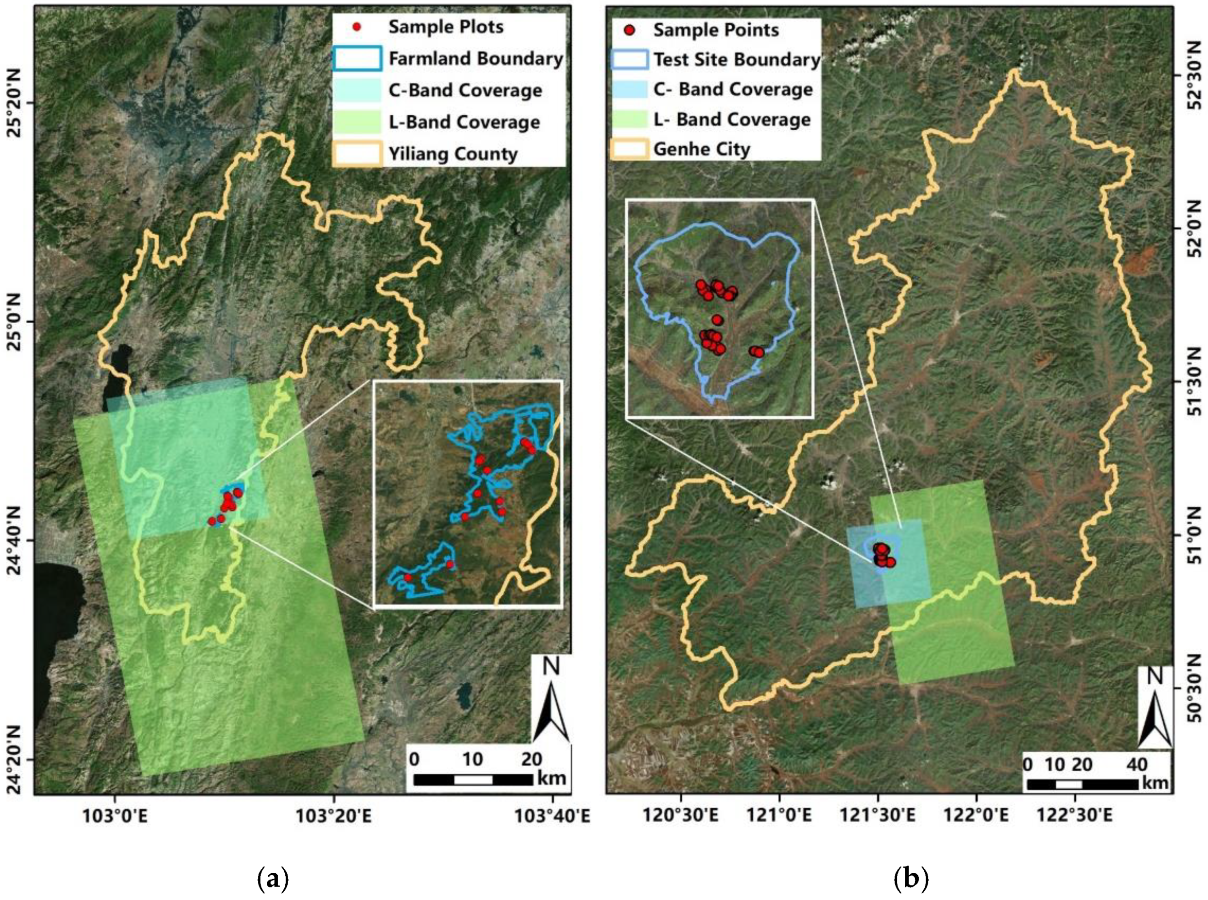
2.1. Test Site

2.1.1. Test Site I

Test site I is the Xiaoshao forest farm (24°39′ to 24°54′ N, 103°02′ to 103°12′ E) in the county of Yiliang in Yunnan province, Southwest China. The elevation varies from 1300 to 2500 m. Most of the plots are located in areas with slopes <30°. The area has a subtropical monsoon climate.

2.1.2. Test Site II

Test site II is located in the high latitude and cold area in Genhe City (50°20′ to 52°30′ N, 120°12′ to 122°55′ E) in the northeast of Hulunbuir League and on the west slope of the north section of Daxinganling, Inner Mongolia, Northeast China. The average altitude is less than 1000 m and with a flat terrain. It has a cold temperate humid forest climate and the characteristics of a continental monsoon climate.

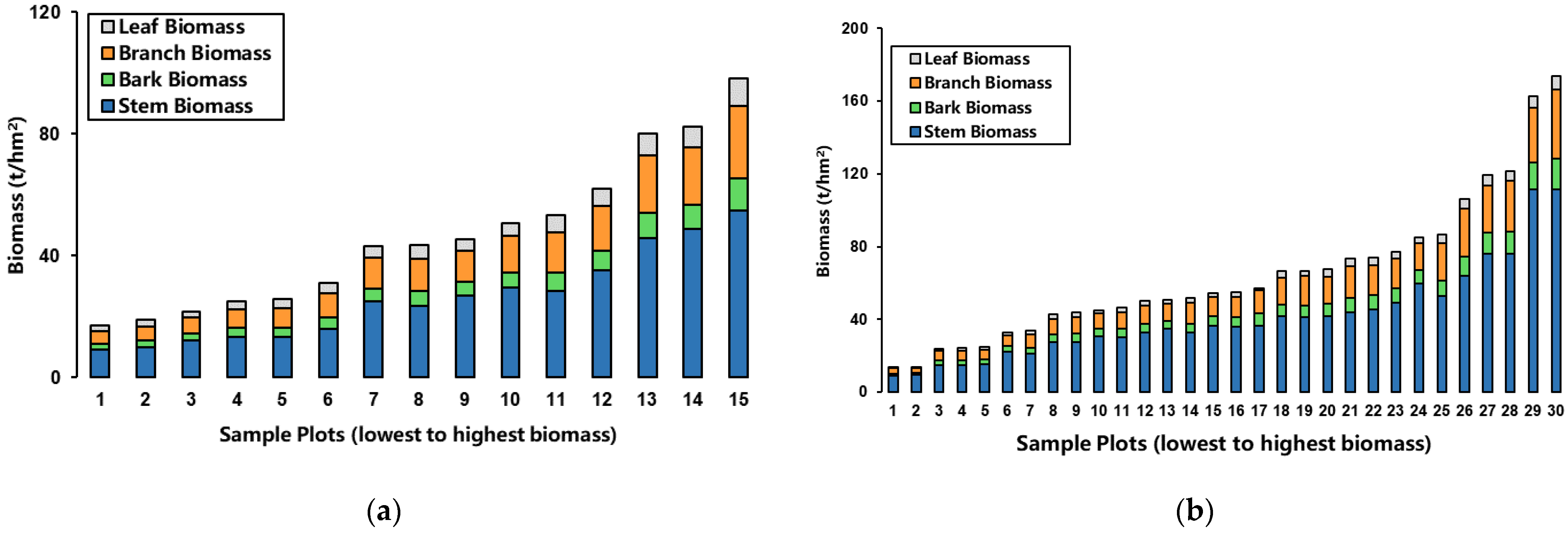
2.2. Plot Measurements

In the field campaign, we recorded tree diameter at breast height (DBH), tree species, and tree height in each plot for the trees with the character of DBH ≥ 5 cm. The sample plots of two test sites were sampled according to a simple random sampling method at the design stage of field work and then several of them were adjusted to be more representative of the forest structure of the study area. Where samples proved difficult to collect during the field campaign due to poor accessibility, the sample sites were changed to make collection easier or abandoned when nearby samples were still not available.
For test site I, the field campaign was conducted in the middle of August, 2019. A total of 15 plots of 25 m × 25 m square stands were investigated. All of the 15 plots were dominated by Pinus yunnanensis.
For test site II, the field campaign was conducted in the middle of August, 2012. A total of 30 plots of 30 m × 30 m square stands were investigated. The dominant tree species in these sample plots were Larix gmelinii, with a few Betula platyphylla and Populus davidiana.
The average AGB value of the sampled plots in test site I was around 50 t/hm2 and the maximum value was less than 150 t/hm2. The average AGB value of the sampled plots in test site II was around 70 t/hm2 and the maximum value was less than 200 t/hm2. The distribution of the plots for the two test sites is shown in Figure 1; Figure 1a is for test site I, while Figure 1b is for test site II. The red plots are the collected sample plots.

2.3. Field-Based AGB Calculation

We calculated total and component AGB using DBH and tree height according to the tree biomass equations shown in Table 1 [29,30,31]. The component biomass values of each tree were totaled to obtain the AGB total amount for all trees in each plot, then the area of each sample plot (0.0625 hm2 for test site I and 0.09 hm2 for test site II) was divided to obtain the total AGB and component biomass of each plot. To eliminate the influence of biomass changes caused by tree growth during the time interval between the sample plot survey and SAR image acquisition, we used the growth pattern models for the corresponding tree species to correct the calculated AGB values of the ground data [32,33,34]. The detailed biomass information for each plot and the distribution of biomass at each component are described in Figure 2.

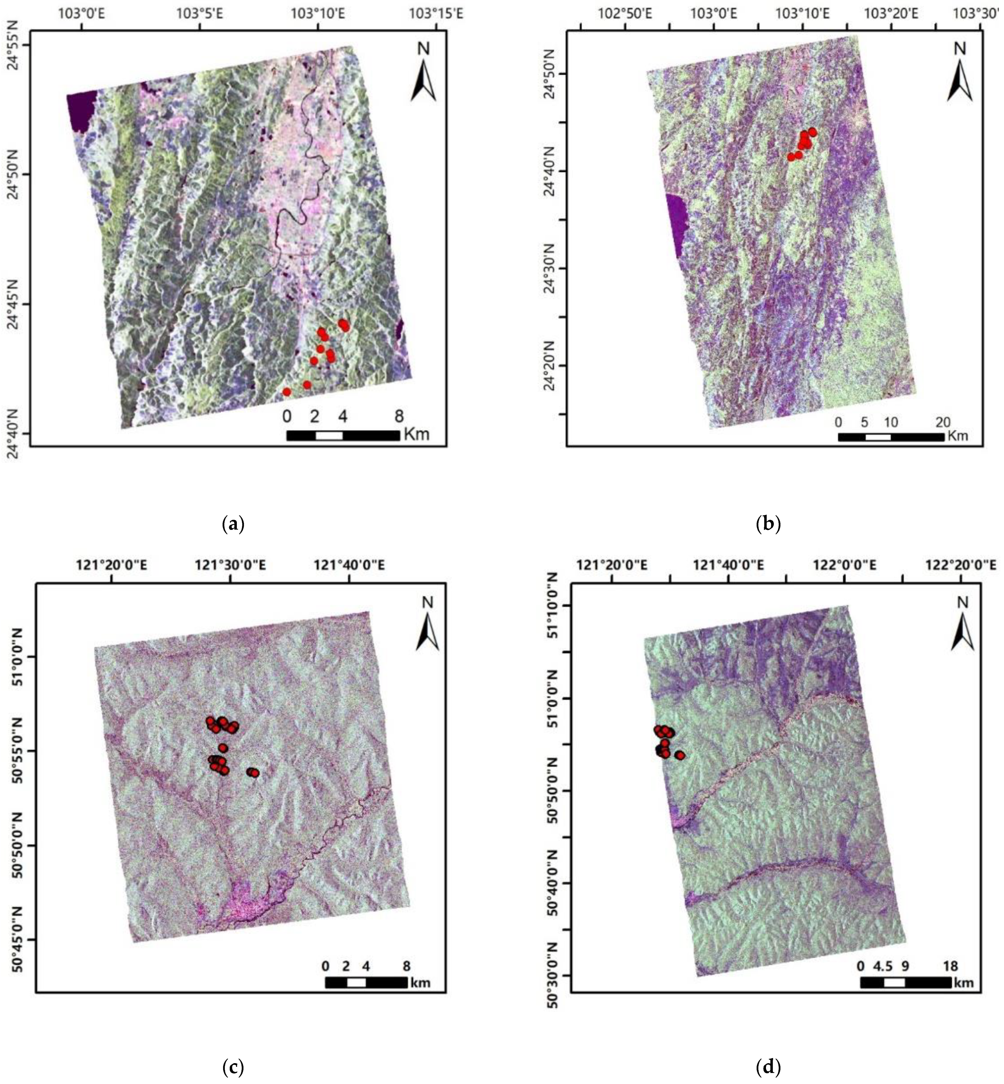
2.4. SAR Data Acquisition and Processing

We acquired a Gaofen-3(GF-3) and an ALOS-2 PALSAR-2 to obtain full polarimetric SAR images covering the study area for test site I and a RADARSAT-2 and an ALOS-2 PALSAR-2 to obtain the images for test site II. Detailed information about the acquired images for the two test sites is shown in Table 2 (test site I) and Table 3 (test site II).
The pre-processing of SAR data was conducted on a computer with the following specifications: Intel Core I7 9750H 2.60 GHz CPU, 16 GB Memory, and an NVIDIA GeForce 1660 Ti GPU. The procedures of SAR data pre-processing included radiometric calibration, speckle filtering, multi-looking, terrain correction, and geocoding. The radiometric calibration, speckle filtering, and multi-looking for the SAR data were performed using PolSARpro software provide by the ESA (European Space Agency), and terrain correction and geocoding were processed using IDL software.
All the images were first radiometrically calibrated to obtain the backscattering coefficients and the scattering matrix (S); the radiometric calibration was carried using the following equation to transform the digital number of each pixel into backscattering coefficients:
For the C-band GF-3 data:
σ d B 0 = 10 log 10 ( P I ( Q V / 32767 ) 2 ) K d B
where P I = I 2 + Q 2 , I and Q are the real and imaginary portions of the level 1A SLC product, respectively, QV is the maximum value of the original image data, which can be found from the QualifyValue in the metadata, and Kdb is the calibration cons in the metadata. For the calibration of C-band RADARSAT-2 data, readers are referred to our previous studies [35,36].
For the L-band ALOS-2 PALSAR-2 data:
σ d B 0 = 10 log 10 ( I 2 + Q 2 ) + C F
where I and Q are the real and imaginary portions of the SLC data and CF is the calibration factor, which is −83 ± 0.406 dB.
After radiometric calibration, the images were speckle filtered and multi-looked with 3 × 3 for PALSAR-2 data, 3 × 3 for GF-3 data, and 2 × 2 for RADARSAT-2 data at range and azimuth directions, respectively. Then, the coherency matrices (T) were obtained. Range-Doppler terrain correction was applied using 30 m Shuttle Radar Topography Mission-1 (SRTM-1) DEM data, the SAR image simulated according to their imaging geometry and available orbit information from the metadata, and the real SAR images were matched to the simulated images, warping to the DEM coordinate system. After the terrain correction, all the SAR images were geocoded into the World Geodetic System-1984 (WGS-84) geographic coordinate system and projected into Universal Transverse Mercator (UTM) map projection (Zone 48N for test site I, Zone 51N for test site II). Next, the SAR parameters corresponding to the sample plot were extracted. Since each sample plot area was 0.0625 or 0.09 ha, we averaged the values of each SAR parameter according to the position relationships between image pixels and the center point of each sample plot. The Pauli RGB color-coded SAR images are shown in Figure 3.

2.5. Polarimetric Parameter Extraction

Since the ground objects in the study area are all woodland and a forest is a complex ecosystem, the ground scattering objects are more complex, and they are basically incoherent targets; therefore, we applied polarimetric decomposition for incoherent targets to the acquired SAR data to extract polarimetric parameters [37]. In this paper, the selected incoherent polarimetric decomposition methods included H/A/Alpha decomposition, Freeman–Durden two-component decomposition (Freeman2), Yamaguchi three-component decomposition (Yamaguchi3), and Target Scattering Vector Model decomposition (TSVM). Table 4 gives the details about the extracted polarimetric parameters.

2.6. Correlation Analysis

Correlation analysis is a statistical method used to express the correlation between two variables by a correlation coefficient. The correlation analysis of the total and component AGB with backscattering and polarimetric information were carried out to explore the relationship between each component biomass and backscattering and polarimetric parameters.

2.7. Parameter Optimal Selection

Parameter optimal selection means selecting a set of parameters with distinguishing properties from a group of parameters according to certain rules. In this study, the total biomass and biomass components were taken as dependent variables, and the backscattering coefficients of four polarization channels at the C- and L-bands and all SAR polarimetric decomposition parameters were taken as the group of independent parameters. We utilized a random forest (RF) algorithm to select the optimal parameters. RF is a machine learning algorithm proposed by Breiman Leo and Adele Cutler in 2001 for classification, regression, and survival analysis [38]. This algorithm can be understood as calculating the importance of features and ranking them. In this study, R language was applied for the performance of RF [39]. For the details of the RF algorithm, readers are referred to the work of Breiman [38].

2.8. Model Building and Evaluation

Regression-based models are the most common biomass estimation approach when using remote sensing data [3]. They have the advantage of flexibility and high interpretability, and many studies have demonstrated their validity for biomass estimation [9,18,23,40]. Therefore, in this study, we selected a multiple linear regression method to build the estimation model. Samples investigated in this study were used for model building and validation. Given the limitations of the small samples, here we used the leave-one-out cross-validation (LOOCV) method to evaluate the capability of the built model [41,42], that is, one sample plot was used as a validation sample each time and other samples were used as training samples for modeling. The process is repeated continuously and all cross-validation results are recorded. Finally, all groups of measured and predicted values were obtained to evaluate the original model. This method can provide unbiased estimation of the true fitting ability of the model and with no data wastage [42]. The coefficient of determination (R2), root mean square error (RMSE), and relative root mean square error (rRMSE in %) were selected to evaluate the model fitting results and estimation results.
R 2 = 1 i = 1 n ( y i y ¯ ) 2 i = 1 n ( Y i y ¯ ) 2
RMSE = 1 n i = 1 n ( Y i y ¯ ) 2
rRMSE = R M S E y ¯ × 100 %
where Y i , y i and y ¯ are measured AGB, predicted AGB, and the mean values of the measured AGB, respectively, and n describes the sample number.

3. Results

3.1. Relating Biomass to Backscattering Coefficients of Each Polarimetric Channel

The correlation analysis was carried out between the backscattering coefficients in the two bands and the total and component AGB of the corresponding sample plots. The results are shown in Table 5 (test site I) and Table 6 (test site II).
For test site I, the values in Table 5 revealed that the backscattering coefficients of each polarimetric channel in the C-band correlated significantly with the total and component AGB at the level of 0.01, the R values indicated that the backscattering of the C-band showed greater sensitivity to the change of biomass in the test site than the L-band. Among them, the C-band HV backscattering coefficient showed a better correlation with total and component AGB than the other three channels. It had the best correlation with the leaf biomass with an R value of 0.831. Next was bark biomass, which was almost the same as that of branch biomass, although the worst correlation was with branch biomass. For other polarimetric channels, the correlations between backscattering coefficients and leaf and branch biomass were also higher than total AGB and stem biomass. The phenomenon revealed the greater sensitivity of C-band backscattering coefficients to the biomass changes in the canopy (branches and leaves).
In test site I, compared with the C-band, each backscattering coefficient of four polarimetric channels of the L-band showed obvious lower sensitivity to both total and each component AGB. Even stem biomass, which usually correlated better with L-band backscattering coefficients in previous studies, also showed a lower correlation with each L-band polarimetric channel backscattering coefficient, with the highest R value being 0.250 obtained via the HV channel. This may result from the different tree species and the forest structure in our study area as compared with previous study areas [43].
Compared to test site I, the R values for the C-band in test site II were lower, but the relationships between HH, VV backscattering coefficients, and biomass were still significant at the 1% level. Meanwhile, HH backscattering coefficients showed the highest correlation with leaf biomass with an R value of 0.532. The relationships between HV, VH backscattering coefficients, and biomass in the L-band were significant at the 1% level, which was better than that obtained at test site I; nonetheless, HH and VV backscattering coefficients showed a poor correlation with total and component biomass.

3.2. Relating Biomass to Polarimetric Decomposition Parameters

The analysis results for the correlations between polarimetric information and forest total and component AGB in this study are shown in Table 7 (test site I) and Table 8 (test site II). Compared with the backscattering coefficients, the correlations between certain polarimetric decomposition parameters and component biomass were obviously increased.
The values in Table 7 revealed that, in test site I, the C-band volume components both from Freeman2 and Yamaguchi3 correlated best with not only total AGB but also each component biomass. Meanwhile, the volume scattering parameter coming from Yamaguchi3 (Yam_Vol3) was more sensitive than that extracted with Freeman2. Next were the Ground (or Dbl) components in these two decomposition methods, which showed better correlation both with total AGB and component biomass. As with the volume component, other parameters extracted from Yamaguchi3 decomposition were better than those extracted from Freeman2. The R value for the C-band volume scattering component of Yamaguchi3 decomposition (Yam3_Vol) was around 0.88, while it was 0.82 for the volume scattering component of the Freeman2 decomposition method (Fre2_Vol). The better performance of Yamaguchi3 parameters may be due to the fact that Yamaguchi modified the volume scattering matrix in the Yamaguchi3 decomposition method according to the relative backscattering magnitudes of the HH channel versus the VV channel. The scattering orientation distribution function of the dipole, which described the dominant scattering objects in the forest canopy, was also modified. The modified volume model seems to be more in accordance with the forest volume scattering in the study area. In addition, the second eigenvector of the TSVM target ellipticity angle (TSVM_tau_m2), Shannon entropy (SE), and its intensity component (SEI) from the C-band were also significantly correlated with the biomass of each fraction.
Among the above-mentioned higher correlations between C-band SAR polarimetric parameters, forest leaf, branch, and bark biomass correlated better with the volume scattering component than with other parts and total AGB. The reason for high correlation between bark biomass and polarimetric SAR parameters needs to be further explored, while the high correlation between leaf and branch biomass and the polarimetric SAR parameters confirmed that the dominant volume scattering mechanism at the C-band came from the forest canopy, while the lower values of R for the correlation between the Dbl component and each component biomass revealed that the Dbl mechanism at the C-band may occur at tree needles, branch, and stem. However, since most of the R values at the L-band did not reach the significance level, we think that the L-band backscatter and polarimetric parameters are disadvantaged for biomass estimation in test site I.
As for test site II, the values in Table 8 revealed that C-band Shannon entropy and components from Freeman2 and Yamaguchi3 decomposition also performed as well as they did in test site I, even with a lower R value. Meanwhile, the L-band polarimetric decomposition parameters performed better in study area II; the Freeman2 ground scattering component (Fre2_Grd), the Yamaguchi3 volume scattering component (Yam3_Vol), and the second eigenvector of the TSVM target phase angle (TSVM_phi_s2) from the L-band all correlated significantly with biomass at the 5% level.

3.3. Optimal Selected Parameters

Table 9 listed the top five parameters which were most important for forest total AGB and component biomass estimation. The order of their importance was determined by the RF optimal parameter selection procedure. The selected features in Table 9 revealed that C-band polarimetric parameters performed better in test site I for estimation of total AGB and for each component biomass, while for test site II, Table 9 shows that the polarimetric parameters both from the C- and L-bands were sensitive for retrieving total AGB and all biomass components. The phenomenon may result from the different forest structures in the two test sites. For test site I, the trees were younger and the forest canopy is more open than that at test site II, meanwhile the average AGB is also lower than that of test site II; the C-band has deeper penetration in test site I and showed better performance than in test site II.

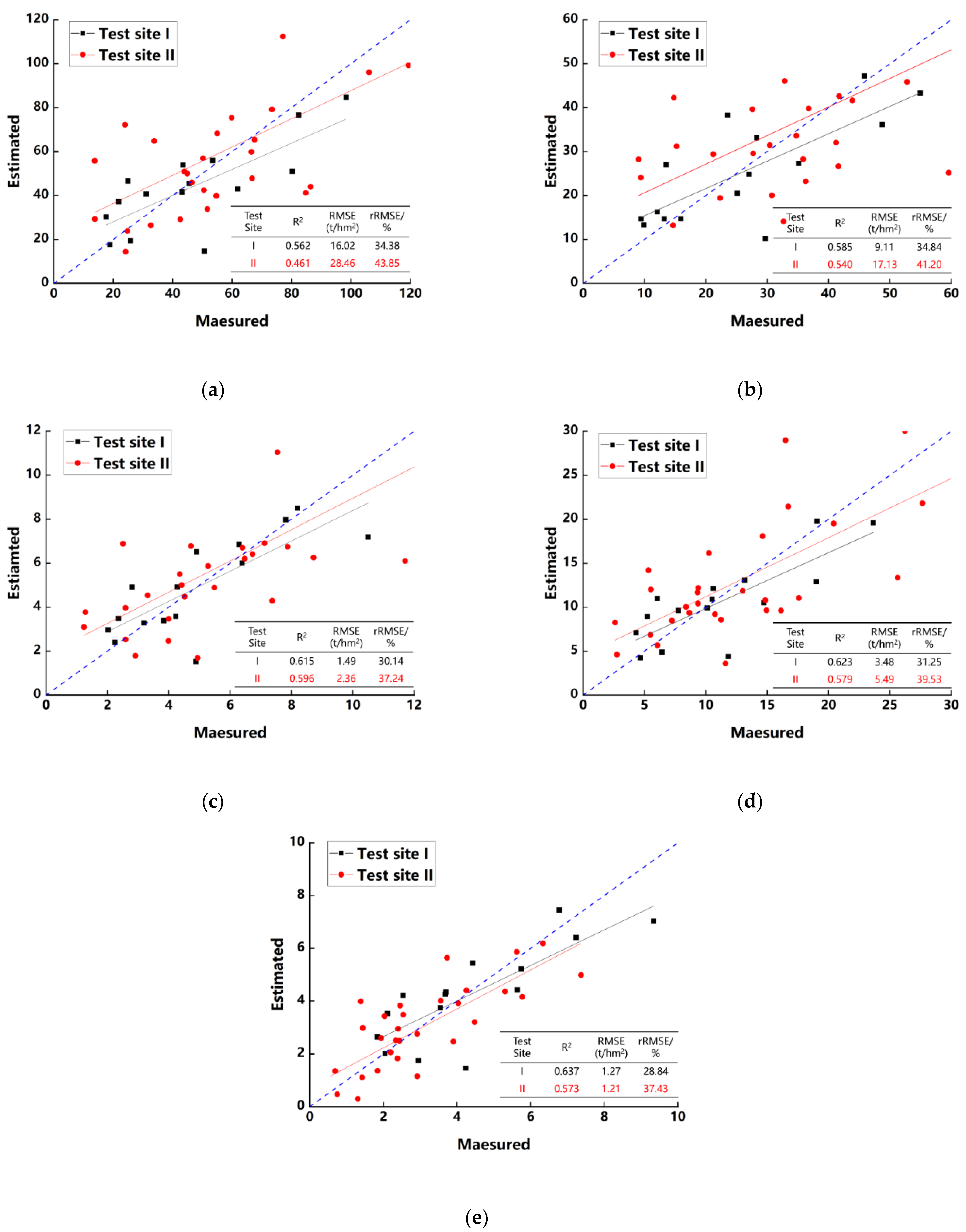
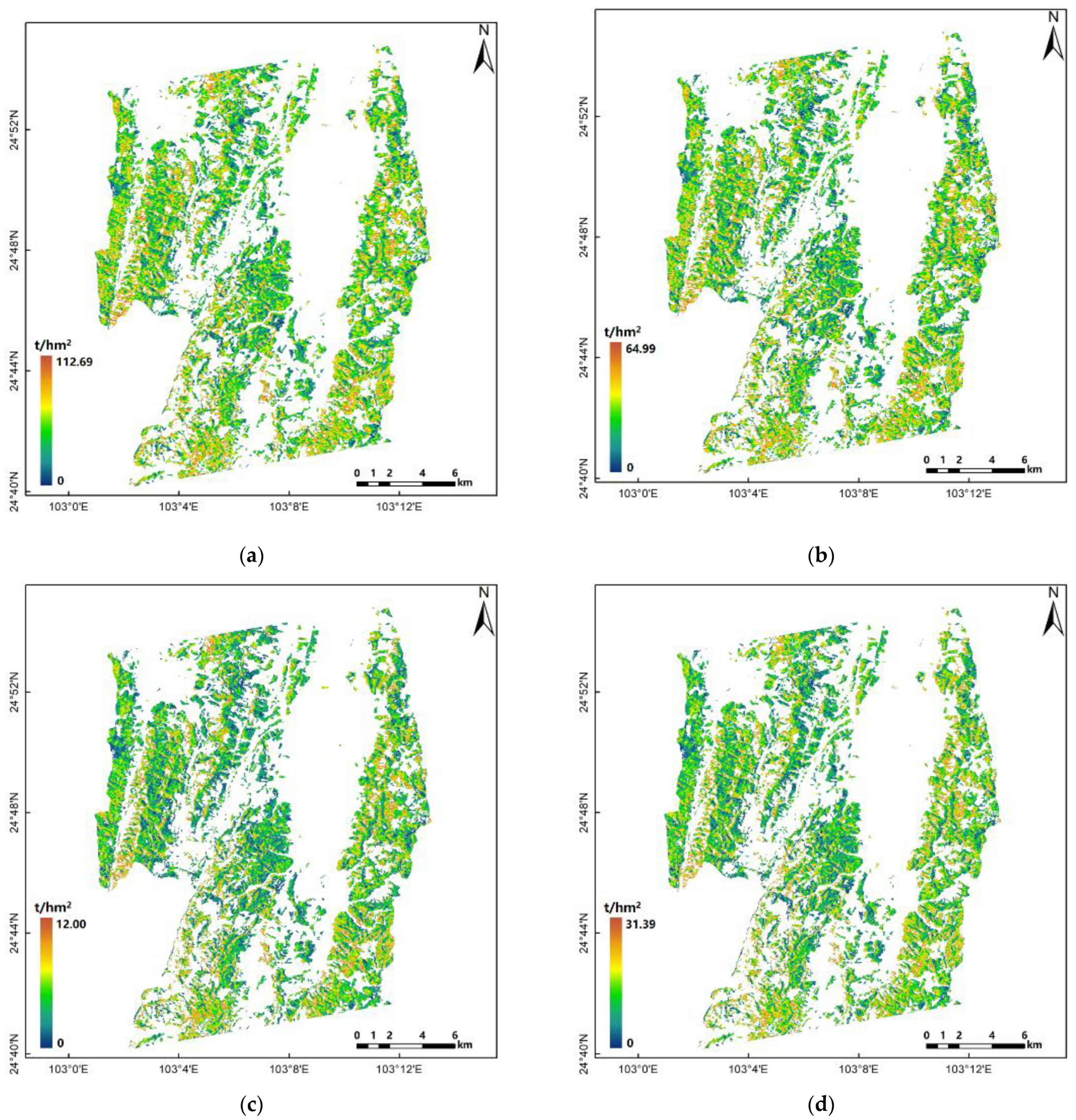
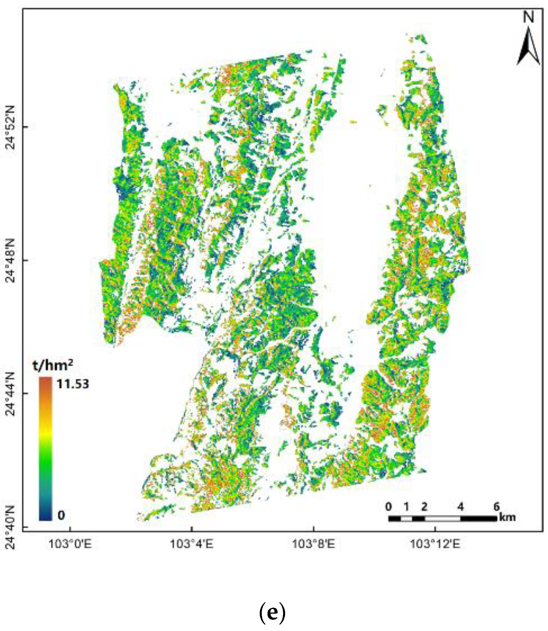
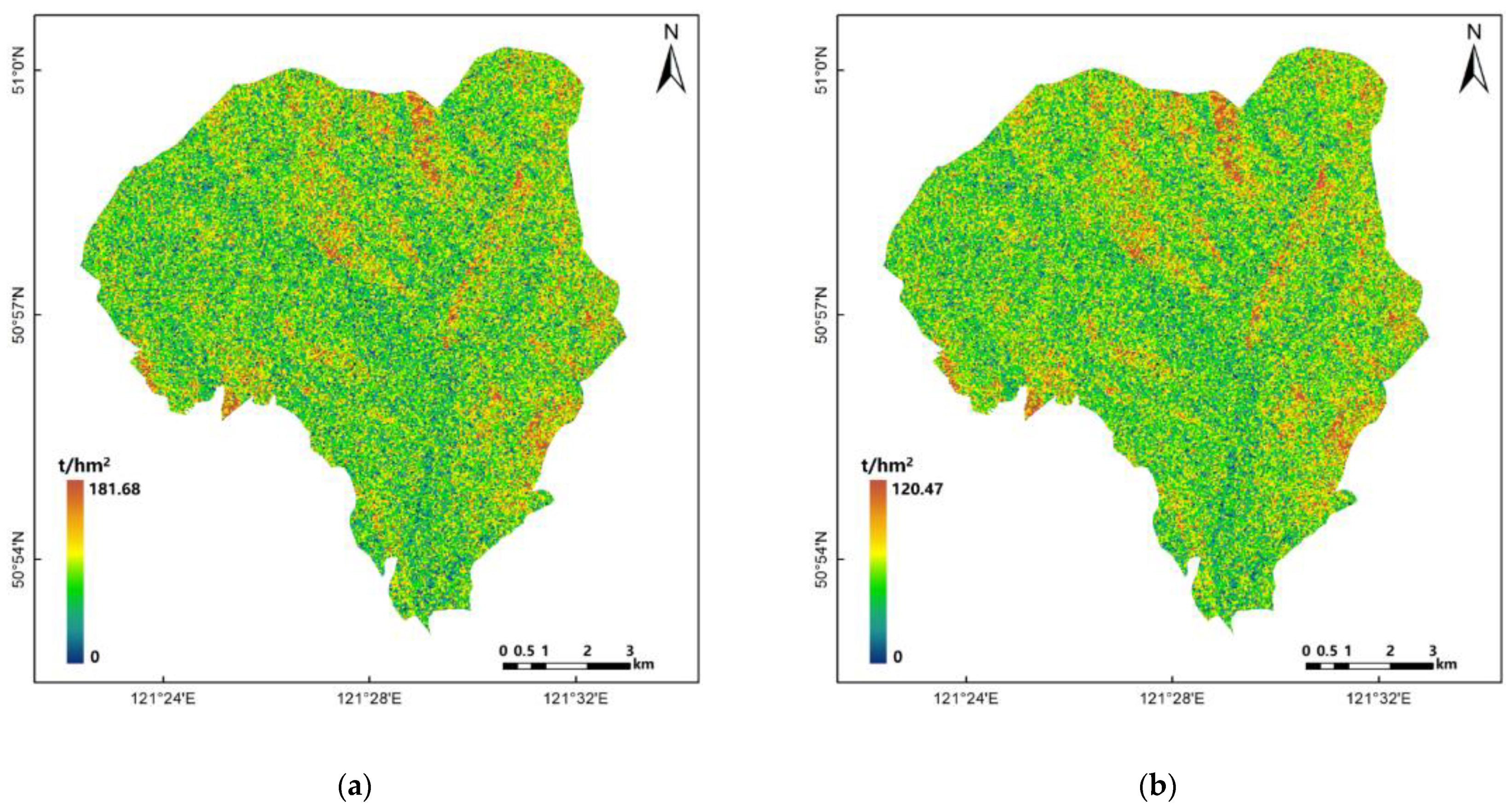
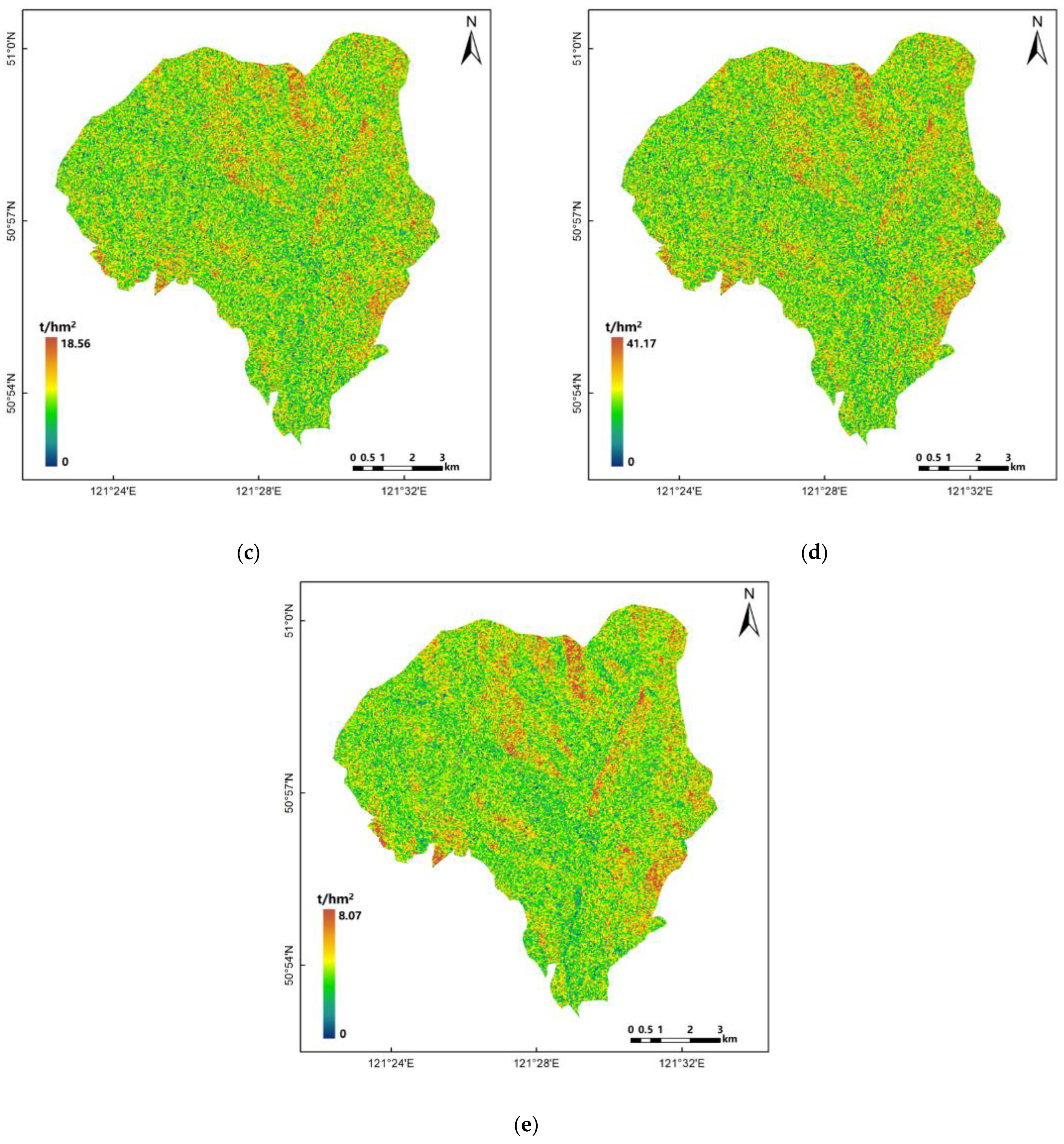
3.4. Forest AGB Estimation and Validation

Figure 4 provides a summary of the validation results of the regression model established with the optimized parameters. For test site I, the model of leaf biomass had the highest accuracy, with R2 = 0.637, RMSE =1.49 t/hm2, and rRMSE = 28.84%. For branch biomass, which was similar to leaf biomass, with a R2 = 0.623, RMSE = 3.48 t/hm2, and rRMSE = 31.25%. The model of total AGB had the lowest accuracy, with R2 = 0.562, RMSE = 16.02 t/hm2, and rRMSE = 34.38%. For test site II, the model of bark biomass had the highest accuracy, with R2 = 0.596, RMSE = 2.36 t/hm2 and rRMSE = 37.24%. Estimation models for branch and leaf biomass performed similar to the bark biomass model; the values of rRMSE were 39.53% and 37.43%, respectively. As for stem biomass, the R2, RMSE, and rRMSE values of the model were 0.540, 17.13 t/hm2, and 41.20%, respectively. The accuracies of each biomass model built for test site II were slightly lower compared to those for test site I.
The distribution maps of total AGB and component biomass for the two test sites were generated and shown here in Figure 5 (test site I) and Figure 6 (test site II). The AGB maps modelled by each component and total retrieval models showed a few overestimations; the areas with overestimated AGB were almost similar for total AGB, stem, bark, branch, and leaf biomass. Most of these areas in both test sites were located in forest areas with higher AGB levels.

4. Discussion

This study utilized the backscatter and polarimetric decomposition parameters extracted from C- and L-band data to estimate forest total AGB and component biomass of Pinus yunnanensis and Larix gmelinii. In test site I, SAR parameters extracted from the C-band showed better performance than those from the L-band for both total and component AGB inversion. The results were in conformity with our previous study in the same study area but where we used a different inversion model [44]. However, they differed from the results mentioned in the research of Kasischke et al. and Cronin et al. [13,22]. In their research, the L-band showed better performance than the C-band. The phenomenon may result from the low biomass level, poor stand structure, and terrain influence in our study area. Le Toan et al. demonstrated that direct volume scattering occurring at the crown having a much smaller scattering component would be stronger than that at a crown with a bigger component and larger canopy gaps, while Dbl would be stronger in lower trees with short scattering waves and higher trees with longer scattering waves [11]. The study of Santoro et al. also addressed the great influence of forest structure on SAR backscattering coefficients [45].
For the SAR backscatter coefficients, in test site I, HV channel backscattering coefficients both at the C- and L-bands correlated best with total AGB and component biomass. For each component biomass, leaf biomass showed the highest correlation with HV channel backscattering coefficients both at the C- and L-bands. R values for these were 0.831 and 0.275, respectively. Stem biomass showed the lowest correlation with HV channel backscattering coefficients with the R = 0.817 and R = 0.204, respectively. The study of [13] also determined that HV channel backscattering coefficients at both the C- and L-bands showed the greatest sensitivity to forest biomass compared to other polarimetric channels.
For polarimetric parameters, volume scattering and double-bounce components both at the C- and L-bands showed obvious high correlations with total and component AGB, especially for test site I. The R values were slightly higher than those in the other study with GF-3 C-band data and similar polarimetric parameters. For example, R values for the correlation between crown biomass and Freeman3 and Yamaguchi3 volume scattering components reported by [23] were 0.68 and 0.74 with significance at the 0.01 level, respectively. Compared with previous studies using Freeman3 to retrieve total AGB, the R values for the correlation between total AGB and surface scattering, double-bounce, and volume scattering components were 0.49, 0.63, and 0.61 respectively. The values were lower than for the same C-band polarimetric components but higher than the L-band components in our study area [18]. The better performance of Yamaguchi3 compared with Freeman2 may be due to the fact that the volume scattering modelling in Yamaguchi3 was improved by adding variable coefficients into the volume scattering model, and the addition of variable coefficients could describe the forest vertical structure information more accurately [46]. The results were also confirmed with the results of [19,20]. However, the correlation between each polarimetric decomposition component and GSV differed from the results obtained from our study area. The results from that study showed higher correlations between volume scattering and surface scattering components with GSV (R = 0.473 and R = 0.732), while in this study, volume scattering and double-bounce scattering components showed better correlations with forest total AGB and component biomass. The phenomenon may have resulted from the difference in tree species and forest structure. Although the Dbl components from Freeman2 and Yamaguchi3 were not correlated as significantly as volume scattering components, they had better correlations to each biomass component. The better performance of the Yamaguchi3 Dbl component in correlating with crown biomass in the artificial forest was also confirmed in the study of [23]. In test site II, parameters exacted from TSVM decomposition, such as the target ellipticity angle (τ) of the eigenvector of TSVM decomposition (TSVM_tau), presented the relative importance in the models. Parameters from the TSVM decomposition were commonly reported to present important information for modelling AGB in the tropics [47,48,49]. Similarly, Shannon entropy and its components were relatively important in the AGB inversion of tropical forests [49,50]. Few studies have been reported on the inversion of AGB in subtropical forests and temperate forests using the above parameters, and the role of parameters from the TSVM decomposition method and Shannon entropy (SE) for the estimation of forest AGB in this region needs to be further explored. The multiple linear regression models showed good performance for total and component biomass estimation in our study. Previous studies also demonstrated the efficiency of multiple linear regression models in forest parameter estimation [9,18,23,40]. Although high rRMSE values were obtained in this study, the error levels were still within the range of similar studies using C-band data. For example, the results obtained by Tsui et al. ranged from 44.0% to 53.6%, while rRMSE values in our study changed from 29.03% to 33.55% [9]. Moreover, the component biomass estimation in this study and in the study of [23] all demonstrated that using polarimetric parameters to invert component biomass showed no obvious saturation phenomenon. This reveals that the method used in this study has potential to improve forest AGB inversion accuracy and saturation levels.

5. Conclusions

This study explored the potential of using backscatter coefficients at different polarimetric channels and polarimetric parameters extracted from C- and L-band full polarimetric SAR data to estimate forest total and component AGB. Through correlation analysis, parameter optimal selection, and a biomass inversion procedure, it is concluded that: (1) adding polarimetric features can improve biomass estimation accuracy both for total and component AGB. Several polarimetric parameters showed better performance than the best backscatter coefficient in the estimation of total and component AGB; (2) the performance of C- and L-band polarimetric observations showed obvious site-dependence during forest total and component AGB estimation. The C-band performed better in more open forests with lower AGB and the L-band performed better in closer forests with moderate AGB levels; (3) for forest component biomass, especially for canopy components, such as branch and leaf biomass, polarimetric features with better performance showed no obvious saturation phenomenon. However, due to the limitation of the collected field sample plots, only 15 sample plots for test site I and 30 sample plots for test site II were used for modelling in this study. Although the results are persuasive, more diverse observational data are needed for verification. Furthermore, in this study only four methods of polarimetric decomposition were used for polarimetric parameter extraction; in the future, other polarimetric parameters extracted by different methods need to be further explored.

Author Contributions

Conceptualization, W.Z.; methodology, P.Z.; project administration, W.Z.; resources, Z.W.; software, P.Z., Y.L. and Z.W.; supervision, W.Z.; validation, P.Z. and J.S.; writing—original draft preparation, P.Z.; writing—review and editing, W.Z., P.Z. and Z.W.; visualization, P.Z. All authors have read and agreed to the published version of the manuscript.

Funding

This research was funded by the Open Research Fund of the Key Laboratory of Earth Observation of Hainan Province, Hainan Research Institute, Aerospace Information Research Institute, Chinese Academy of Sciences, grant number 2020LDE003; the National Natural Science Foundation of China, grant numbers 31860240, 32160365, and 42161059; and the Cultivating Plan Program for the Leader in Science and Technology of Yunnan Province (CN), grant number 80201444.

Institutional Review Board Statement

Not applicable.

Informed Consent Statement

Not applicable.

Data Availability Statement

The datasets analyzed during the current study are available from the Institute of Forest Resources Information Technique, Chinese Academy of Forestry, but restrictions apply to the availability of these data and so they are not publicly available.

Acknowledgments

The authors would like to thank the European Space Agency (https://www.esa.int/, accessed on 11 January 2022) for providing the Polarimetric SAR Data Processing and Educational Toolbox (PolSARpro) software for effectively manipulating the SAR data. The authors also would like to acknowledge the Japan Aerospace Exploration Agency for its Earth Observations (EORA2) projects for the acquired ALOS-2 PALSAR-2 images in this study.

Conflicts of Interest

The authors declare no conflict of interest.

References

  1. Wang, Y.; Pyörälä, J.; Liang, X.; Lehtomäki, M.; Kukko, A.; Yu, X.; Kaartinen, H.; Hyyppä, J. In Situ Biomass Estimation at Tree and Plot Levels: What Did Data Record and What Did Algorithms Derive from Terrestrial and Aerial Point Clouds in Boreal Forest. Remote Sens. Environ. 2019, 232, 111309. [Google Scholar] [CrossRef]
  2. Santoro, M.; Cartus, O.; Fransson, J.E.S.; Wegmüller, U. Complementarity of X-, C-, and L-Band SAR Backscatter Observations to Retrieve Forest Stem Volume in Boreal Forest. Remote Sens. 2019, 11, 1563. [Google Scholar] [CrossRef] [Green Version]
  3. Lu, D.; Chen, Q.; Wang, G.; Liu, L.; Li, G.; Moran, E. A Survey of Remote Sensing-Based Aboveground Biomass Estimation Methods in Forest Ecosystems. Int. J. Digit. Earth 2016, 9, 63–105. [Google Scholar] [CrossRef]
  4. Hayashi, M.; Motohka, T.; Sawada, Y. Aboveground Biomass Mapping Using ALOS-2/PALSAR-2 Time-Series Images for Borneo’s Forest. IEEE J. Sel. Top. Appl. Earth Obs. Remote Sens. 2019, 12, 5167–5177. [Google Scholar] [CrossRef]
  5. Gallaun, H.; Zanchi, G.; Nabuurs, G.-J.; Hengeveld, G.; Schardt, M.; Verkerk, P.J. EU-Wide Maps of Growing Stock and above-Ground Biomass in Forests Based on Remote Sensing and Field Measurements. For. Ecol. Manag. 2010, 260, 252–261. [Google Scholar] [CrossRef]
  6. Baccini, A.; Goetz, S.J.; Walker, W.S.; Laporte, N.T.; Sun, M.; Sulla-Menashe, D.; Hackler, J.; Beck, P.S.A.; Dubayah, R.; Friedl, M.A.; et al. Estimated Carbon Dioxide Emissions from Tropical Deforestation Improved by Carbon-Density Maps. Nat. Clim. Change 2012, 2, 182–185. [Google Scholar] [CrossRef]
  7. Kellndorfer, J.M.; Dubayah, R.; Siqueira, P.; Saatchi, S.S.; Chapman, B.D.; Rosen, P.A. Large-Scale Mapping and Monitoring of Terrestrial Ecosystems with the NISAR Mission. In Proceedings of the AGU Fall Meeting 2014, San Francisco, CA, USA, 15–19 December 2014. [Google Scholar]
  8. Lambert, M.-C.; Ung, C.-H.; Raulier, F. Canadian National Tree Aboveground Biomass Equations. Can. J. For. Res. 2005, 35, 1996–2018. [Google Scholar] [CrossRef]
  9. Tsui, O.W.; Coops, N.C.; Wulder, M.A.; Marshall, P.L.; McCardle, A. Using Multi-Frequency Radar and Discrete-Return LiDAR Measurements to Estimate above-Ground Biomass and Biomass Components in a Coastal Temperate Forest. ISPRS J. Photogramm. Remote Sens. 2012, 69, 121–133. [Google Scholar] [CrossRef]
  10. Saatchi, S.; Halligan, K.; Despain, D.G.; Crabtree, R.L. Estimation of Forest Fuel Load From Radar Remote Sensing. IEEE Trans. Geosci. Remote Sens. 2007, 45, 1726–1740. [Google Scholar] [CrossRef]
  11. Le Toan, T.; Beaudoin, A.; Riom, J.; Guyon, D. Relating Forest Biomass to SAR Data. IEEE Trans. Geosci. Remote Sens. 1992, 30, 403–411. [Google Scholar] [CrossRef]
  12. Dobson, M.C.; Ulaby, F.T.; LeToan, T.; Beaudoin, A.; Kasischke, E.S.; Christensen, N. Dependence of Radar Backscatter on Coniferous Forest Biomass. IEEE Trans. Geosci. Remote Sens. 1992, 30, 412–415. [Google Scholar] [CrossRef]
  13. Kasischke, E.S.; Christensen, N.L.; Bourgeau-Chavez, L.L. Correlating Radar Backscatter with Components of Biomass in Loblolly Pine Forests. IEEE Trans. Geosci. Remote Sens. 1995, 33, 643–659. [Google Scholar] [CrossRef]
  14. Peregon, A.; Yamagata, Y. The Use of ALOS/PALSAR Backscatter to Estimate above-Ground Forest Biomass: A Case Study in Western Siberia. Remote Sens. Environ. 2013, 137, 139–146. [Google Scholar] [CrossRef]
  15. Stelmaszczuk-Górska, M.; Urbazaev, M.; Schmullius, C.; Thiel, C. Estimation of Above-Ground Biomass over Boreal Forests on Siberia Using Updated In Situ, ALOS-2 PALSAR-2, and RADARSAT-2 Data. Remote Sens. 2018, 10, 1550. [Google Scholar] [CrossRef] [Green Version]
  16. Monteith, A.R.; Ulander, L.M.H. Temporal Characteristics of P-Band Tomographic Radar Backscatter of a Boreal Forest. IEEE J. Sel. Top. Appl. Earth Obs. Remote Sens. 2021, 14, 1967–1984. [Google Scholar] [CrossRef]
  17. Garestier, F.; Dubois-Fernandez, P.C.; Guyon, D.; Le Toan, T. Forest Biophysical Parameter Estimation Using L- and P-Band Polarimetric SAR Data. IEEE Trans. Geosci. Remote Sens. 2009, 47, 3379–3388. [Google Scholar] [CrossRef]
  18. Gonçalves, F.G.; Santos, J.R.; Treuhaft, R.N. Stem Volume of Tropical Forests from Polarimetric Radar. Int. J. Remote Sens. 2011, 32, 503–522. [Google Scholar] [CrossRef]
  19. Kobayashi, S.; Omura, Y.; Sanga-Ngoie, K.; Widyorini, R.; Kawai, S.; Supriadi, B.; Yamaguchi, Y. Characteristics of Decomposition Powers of L-Band Multi-Polarimetric SAR in Assessing Tree Growth of Industrial Plantation Forests in the Tropics. Remote Sens. 2012, 4, 3058–3077. [Google Scholar] [CrossRef] [Green Version]
  20. Chowdhury, T.; Thiel, C.; Schmullius, C.; Stelmaszczuk-Górska, M. Polarimetric Parameters for Growing Stock Volume Estimation Using ALOS PALSAR L-Band Data over Siberian Forests. Remote Sens. 2013, 5, 5725–5756. [Google Scholar] [CrossRef] [Green Version]
  21. Dobson, M.C.; Ulaby, F.T.; Pierce, L.E.; Sharik, T.L.; Bergen, K.M.; Kellndorfer, J.; Kendra, J.R.; Li, E.; Lin, Y.C.; Nashashibi, A.; et al. Estimation of Forest Biophysical Characteristics in Northern Michigan with SIR-C/X-SAR. IEEE Trans. Geosci. Remote Sens. 1995, 33, 877–895. [Google Scholar] [CrossRef]
  22. Cronin, N.; Lucas, R.M.; Milne, A.K.; Witte, C. Relationships between the Component Biomass of Woodlands in Australia and Data from Airborne and Spaceborne SAR. IEEE 2000, 4, 1393–1395. [Google Scholar]
  23. Wei, J.; Fan, W.; Yu, Y.; Mao, X. Polarimetric Decomposition Parameters for Artificial Forest Canopy Biomass Estimation Using GF-3 Fully Polarimetric SAR Data. Sci. Silvae Sin. 2020, 56, 174–183. (In Chinese) [Google Scholar] [CrossRef]
  24. Cheng, S.; Xu, Z.; Su, Y.; Zhen, L. Spatial and Temporal Flows of China’s Forest Resources: Development of a Framework for Evaluating Resource Efficiency. Ecol. Econ. 2010, 69, 1405–1415. [Google Scholar] [CrossRef]
  25. Cai, H.; Yang, X.; Wang, K.; Xiao, L. Is Forest Restoration in the Southwest China Karst Promoted Mainly by Climate Change or Human-Induced Factors? Remote Sens. 2014, 6, 9895–9910. [Google Scholar] [CrossRef] [Green Version]
  26. Hu, T.; Hu, H.; Li, F.; Zhao, B.; Wu, S.; Zhu, G.; Sun, L. Long-Term Effects of Post-Fire Restoration Types on Nitrogen Mineralisation in a Dahurian Larch (Larix Gmelinii) Forest in Boreal China. Sci. Total Environ. 2019, 679, 237–247. [Google Scholar] [CrossRef]
  27. Song, Q.; Fan, W. ALOS PALSAR Estimation of Vegetation Biomass in Daxing’anling Region. Chin. J. Appl. Ecol. 2011, 22, 303–308. (In Chinese) [Google Scholar]
  28. Li, M.; Yu, X.; Gao, Y.; Fan, W. Remote Sensing Quantification on Forest Biomass Based on SAR Polarization Decompositon and Landsat Data. J. Beijing For. Univ. 2018, 40, 1–10. (In Chinese) [Google Scholar] [CrossRef]
  29. State Forestry Administration of China. Tree Biomass Models and Related Parameters to Carbon Accounting for Pinus yunnanensis; State Forestry Administration of China: Beijing, China, 2014; pp. 2–3. (In Chinese)
  30. State Forestry Administration of China. Tree Biomass Models and Related Parameters to Carbon Accounting for Larix gmelinii; State Forestry Administration of China: Beijing, China, 2016; pp. 2–6. (In Chinese)
  31. State Forestry Administration of China. Tree Biomass Models and Related Parameters to Carbon Accounting for Betula platyphylla; State Forestry Administration of China: Beijing, China, 2016; pp. 2–6. (In Chinese)
  32. Li, B.; Liu, Z.; Wang, L. A Primary Study on the Structure of the Forest Stands of Forest of Pinus Yunnanensis and the Regular Pattern of Its Development. J. Yunnan Univ. Nat. Sci. 1984, 01, 47–58. (In Chinese) [Google Scholar]
  33. Zhang, J.; Sun, Y.; Xu, J. Research on Growing Process of Larix Gmeini Plantation in Northeast of China. J. Northwest For. Univ. 2008, 23, 179–181. (In Chinese) [Google Scholar]
  34. Wang, L.; Wang, L. The Growth Model of DBH of Birch Based on Quantitative Theory. Anhui Agri. Sci. Bull. 2016, 22, 89–99. (In Chinese) [Google Scholar] [CrossRef]
  35. Zhang, W.; Li, Z.; Chen, E.; Zhang, Y.; Yang, H.; Zhao, L.; Ji, Y. Compact Polarimetric Response of Rape (Brassica Napus L.) at C-Band: Analysis and Growth Parameters Inversion. Remote Sens. 2017, 9, 591. [Google Scholar] [CrossRef] [Green Version]
  36. Zhang, W.; Chen, E.; Li, Z.; Zhao, L.; Ji, Y.; Zhang, Y.; Liu, Z. Rape (Brassica Napus L.) Growth Monitoring and Mapping Based on Radarsat-2 Time-Series Data. Remote Sens. 2018, 10, 206. [Google Scholar] [CrossRef] [Green Version]
  37. Cloude, S.R.; Pottier, E. A Review of Target Decomposition Theorems in Radar Polarimetry. IEEE Trans. Geosci. Remote Sens. 1996, 34, 498–518. [Google Scholar] [CrossRef]
  38. Breiman, L. Random Forests. Mach. Learn. 2001, 45, 5–32. [Google Scholar] [CrossRef] [Green Version]
  39. R Core Team. R: A Language and Environment for Statistical Computing; R Foundation for Statistical Computing: Vienna, Austria, 2020. [Google Scholar]
  40. He, Q.; Chen, E.; An, R.; Li, Y. Above-Ground Biomass and Biomass Components Estimation Using LiDAR Data in a Coniferous Forest. Forests 2013, 4, 984–1002. [Google Scholar] [CrossRef] [Green Version]
  41. Stone, M. Cross-Validatory Choice and Assessment of Statistical Predictions. J. R. Stat. Soc. Ser. B Methodol. 1974, 36, 111–133. [Google Scholar] [CrossRef]
  42. Cawley, G.C.; Talbot, N.L.C. Fast Exact Leave-One-out Cross-Validation of Sparse Least-Squares Support Vector Machines. Neural Netw. 2004, 17, 1467–1475. [Google Scholar] [CrossRef]
  43. Imhoff, M.L. Radar Backscatter and Biomass Saturation: Ramifications for Global Biomass Inventory. IEEE Trans. Geosci. Remote Sens. 1995, 33, 511–518. [Google Scholar] [CrossRef]
  44. Ji, Y.; Xu, K.; Zeng, P.; Zhang, W. GA-SVR Algorithm for Improving Forest above Ground Biomass Estimation Using SAR Data. IEEE J. Sel. Top. Appl. Earth Obs. Remote Sens. 2021, 14, 6585–6595. [Google Scholar] [CrossRef]
  45. Santoro, M.; Fransson, J.E.S.; Eriksson, L.E.B.; Magnusson, M.; Ulander, L.M.H.; Olsson, H. Signatures of ALOS PALSAR L-Band Backscatter in Swedish Forest. IEEE Trans. Geosci. Remote Sens. 2009, 47, 4001–4019. [Google Scholar] [CrossRef] [Green Version]
  46. Cui, Y.; Yamaguchi, Y.; Yang, J.; Park, S.-E.; Kobayashi, H.; Singh, G. Three-Component Power Decomposition for Polarimetric SAR Data Based on Adaptive Volume Scatter Modeling. Remote Sens. 2012, 4, 1559–1572. [Google Scholar] [CrossRef] [Green Version]
  47. Baker, T.R.; Phillips, O.L.; Malhi, Y.; Almeida, S.; Arroyo, L.; Di Fiore, A.; Erwin, T.; Killeen, T.J.; Laurance, S.G.; Laurance, W.F.; et al. Variation in Wood Density Determines Spatial Patterns InAmazonian Forest Biomass: Wood Specific Gravity and Amazonian Biomass Estimates. Glob. Change Biol. 2004, 10, 545–562. [Google Scholar] [CrossRef]
  48. Bispo, P.C.; Santos, J.R.; Valeriano, M.M.; Touzi, R.; Seifert, F.M. Integration of Polarimetric PALSAR Attributes and Local Geomorphometric Variables Derived from SRTM for Forest Biomass Modeling in Central Amazonia. Can. J. Remote Sens. 2014, 40, 26–42. [Google Scholar] [CrossRef]
  49. Cassol, H.L.G.; Carreiras, J.M.; Moraes, E.C.; Aragão, L.E.; Silva, C.V.; Quegan, S.; Shimabukuro, Y.E. Retrieving Secondary Forest Aboveground Biomass from Polarimetric ALOS-2 PALSAR-2 Data in the Brazilian Amazon. Remote Sens. 2018, 11, 59. [Google Scholar] [CrossRef] [Green Version]
  50. Godinho Cassol, H.L.; De Oliveira E Cruz De Aragão, L.E.; Moraes, E.C.; De Brito Carreiras, J.M.; Shimabukuro, Y.E. Quad-Pol Advanced Land Observing Satellite/Phased Array L-Band Synthetic Aperture Radar-2 (ALOS/PALSAR-2) Data for Modelling Secondary Forest above-Ground Biomass in the Central Brazilian Amazon. Int. J. Remote Sens. 2021, 42, 4985–5009. [Google Scholar] [CrossRef]
Figure 1. The test sites and the distribution maps of the collected stands for (a) test site I and (b) test site II.
Forests 13 00442 g001
Figure 2. The distribution of component biomass for each plot: (a) test site I; (b) test site II.
Forests 13 00442 g002
Figure 3. Pauli RGB (R:|HH − VV|, G:|HV + VH|, B:|HH + VV|) color-coded images of C-band GF-3 for test site I: (a) L-band ALOS-2 PALSAR-2 for test site I; (b) C-band RADARSAT-2 for test site II; (c) L-band ALOS-2 PALSAR-2 for test site II; (d) the red dots represent the distribution of the ground sample plots.
Forests 13 00442 g003
Figure 4. The validation results of the estimated total AGB and component biomass of test sites: (a) total AGB; (b) stem; (c) bark; (d) branch; (e) leaf.
Forests 13 00442 g004
Figure 5. Generated biomass distribution map for test site I: (a) total AGB; (b) stem; (c) bark; (d) branch; (e) leaf.
Forests 13 00442 g005aForests 13 00442 g005b
Figure 6. Generated biomass distribution map for test site II: (a) total AGB; (b) stem; (c) bark; (d) branch; (e) leaf.
Forests 13 00442 g006aForests 13 00442 g006b
Table 1. Equations of total and component AGB for Pinus yunnanensis, Larix gmelinii, and Betula platyphylla.
AGBModel EquationsDetermination Coefficient
Total AGB (MA, kg)For Pinus yunnanensis: 0.070231DBH2.10392H0.41120
For Larix gmelinii: 0.06848DBH2.01549H0.59145
For Betula platyphylla: 0.06807DBH2.10850H0.52019
For Pinus yunnanensis: 0.9485
For Larix gmelinii: 0.9690
For Betula platyphylla: 0.9550
Stem (MS, kg) M S = 1 1 + g 1 + g 2 + g 3 × M A For Pinus yunnanensis: 0.9494
For Larix gmelinii: 0.9701
For Betula platyphylla: 0.9545
Bark (MB, kg) M B = g 1 1 + g 1 + g 2 + g 3 × M A For Pinus yunnanensis: 0.8724
For Larix gmelinii: 0.8817
For Betula platyphylla: 0.8678
Branch (MBr, kg) M Br = g 2 1 + g 1 + g 2 + g 3 × M A For Pinus yunnanensis: 0.8395
For Larix gmelinii: 0.8513
For Betula platyphylla: 0.9545
Leaf (ML, kg) M L = g 3 1 + g 1 + g 2 + g 3 × M A For Pinus yunnanensis: 0.6540
For Larix gmelinii: 0.7439
For Betula platyphylla: 0.6311
Note: DBH (cm); H is tree height (m); g1, g2 and g3 are proportional functions of bark, branch, and leaf relative to stem biomass of 1, respectively: g1 = 1.50018DBH−0.27008H−0.57857, g2 = 1.93610DBH0.61425H−1.36341, g3 = 2.37294DBH0.43806H−1.65700 for Pinus yunnanensis; g1 = 0.36742DBH0.16892H−0.17313, g2 = 2.30634DBH0.72188H−1.54081, g3 = 1.57804DBH0.19257H−1.36274 for Larix gmelinii; g1 = 0.53498DBH0.09004H−0.46520, g2 = 1.05167DBH0.66925H−1.04662, g3 = 0.61793DBH0.17097H−0.88182 for Betula platyphylla.
Table 2. Detailed information about the SAR images for test site I.
ParametersGF-3ALOS-2 PALSAR-2
Acquired Date18 May 201822 April 2016
Center frequency5.40 GHz1.24 GHz
Incidence angle39.1°33.9°
Resolution (range × azimuth)2.248 m × 5.120 m2.86 m × 3.21 m
Orbit directionAscendingAscending
Observation modeQuad-Polarization Stripmap I (QPSI)High-Sensitive Full Polarization (HBQ)
Table 3. Detailed information about the SAR images for test site II.
ParametersRADARSAT-2ALOS-2 PALSAR-2
Acquired Date20 August 201329 August 2014
Center frequency5.405 GHz1.24 GHz
Incidence angle37.4°36.52°
Resolution (range × azimuth)4.96 m × 4.73 m2.86 m × 2.64 m
Orbit directionAscendingAscending
Observation modeULTRA FINEHigh-Sensitive Full Polarization (HBQ)
Table 4. Polarimetric decomposition parameters.
MethodParameter
Yamaguchi3
decomposition
Volume scattering component of Yamaguchi3 decomposition (Yam3_Vol)
Odd scattering component of Yamaguchi3 decomposition (Yam3_Odd)
Double-bounce component of Yamaguchi3 decomposition (Yam3_Dbl)
Freeman2
decomposition
Scattering component of Yamaguchi3 decomposition (Fre2_Vol)
Ground scattering component of Yamaguchi3 decomposition (Fre2_Grd)
H/A/alpha
decomposition
Mean scattering angle (alpha)
A parameter for assessing the type of symmetry (anisotropy)
Polarimetric scattering entropy (entropy)
Single-Bounce Eigenvalue Relative Difference (SERD)
Double-Bounce Eigenvalue Relative Difference (SERD)
Shannon entropy (SE)
Intensity component of Shannon entropy (SEi)
Polarization degree component of Shannon entropy (SEp)
Polarization Fraction (PF)
Polarization Asymmetry (PA)
Radar Vegetation Index (RVI)
Pedestal Height (PH)
TSVM
decomposition
4 symmetry scattering parameters (TSVM_alpha_s, TSVM_alpha_s1, TSVM_alpha_s2, TSVM_alpha_s3)
4 target phase angle parameters (TSVM_phi_s; TSVM_phi_s1, TSVM_phi_s2, TSVM_phi_s3)
4 target orientation angle parameters (TSVM_psi, TSVM_psi1, TSVM_psi2, TSVM_psi3)
4 target ellipticity angle parameters (TSVM_tau_m, TSVM_tau_m1, TSVM_tau_m2, TSVM_tau_m3)
Table 5. R values between the backscatter coefficients and forest biomass for test site I.
BiomassHH (C)HV (C)VH (C)VV (C)HH (L)HV (L)VH (L)VV (L)
Total0.737 **0.827 **0.805 **0.723 **−0.1730.2240.2430.008
Stem0.724 **0.817 **0.795 **0.720 **−0.1980.2040.229−0.010
Bark0.748 **0.830 **0.811 **0.710 **−0.1150.2650.2690.047
Branch0.742 **0.829 **0.808 **0.722 **−0.1570.2350.2500.018
Leaf0.748 **0.831 **0.812 **0.711 **−0.0990.2750.2750.057
** Represents a significance level at 1% (two-tailed). C and L in brackets mean C- and L-band, respectively.
Table 6. R values between the backscatter coefficients and forest biomass for test site II.
BiomassHH (C)HV (C)VH (C)VV (C)HH (L)HV (L)VH (L)VV (L)
Total0.511 **0.2850.3350.493 **0.2730.473 **0.481 **0.302
Stem0.508 **0.2680.3210.474 **0.2550.455 **0.462 **0.283
Bark0.515 **0.3060.3500.513 **0.2890.488 **0.499 **0.321
Branch0.494 **0.2960.3420.511 **0.2930.488 **0.500 **0.320
Leaf0.532 **0.3330.401 *0.530 **0.2920.481 **0.508 **0.352
* Represents a significance level at 5% (two-tailed). ** Represents a significance level at 1% (two-tailed). C and L in brackets mean C- and L-band, respectively.
Table 7. R values between the polarimetric parameters and forest biomass for test site I.
BiomassFre2_Grd (C)Fre2_Vol (C)Yam3_Dbl (C)Yam3_Odd (C)Yam3_Vol (C)SE (C)SEi (C)TSVM_tau_m2(C)TSVM_psi3(L)
Total0.798 **0.809 **0.814 **0.675 **0.833 **0.781 **0.837 **0.634 *−0.689 **
Stem0.786 **0.795 **0.835 **0.657 **0.863 **0.789 **0.824 **0.626 *−0.683 **
Bark0.810 **0.825 **0.849 **0.703 **0.868 **0.791 **0.850 **0.640 *−0.692 **
Branch0.804 **0.813 **0.805 **0.684 **0.861 **0.794 **0.841 **0.635 *−0.690 **
Leaf0.809 **0.828 **0.809 **0.708 **0.881 **0.801 **0.851 **0.641 *−0.690 **
* Represents significance level at 5% (two-tailed). ** Represents significance level at 1% (two-tailed). C, L in brackets means the C- and L-bands, respectively.
Table 8. R values between the polarimetric parameters and forest biomass for test site II.
BiomassFre2_Vol (C)Yam3_Odd (C)Yam3_Vol (C)SE (C)SEI (C)TSVM_alpha_s1(C)TSVM_tau_m2(C)Fre2_Grd (L)Yam_3_Vol (L)TSVM_phi_s2(L)
Total0.519 **0.378 *0.561 **0.533 **0.481 **−0.458 *−0.549 **0.419 *0.499 **0.554 **
Stem0.511 **0.371 *0.552 **0.523 **0.470 **−0.439 *−0.536 **0.389 *0.484 **0.550 **
Bark0.535 **0.390 *0.569 **0.546 **0.495 **−0.485 **.−0.564 **0.441 *0.510 **0.546 **
Branch0.519 **0.367 *0.557 **0.526 **0.477 **−0.481 **−0.565 **0.474 **0.507 **0.551 **
Leaf0.520 **0.387 *0.580 **0.538 **0.512 **−0.451 *−0.563 **0.396 *0.512 **0.496 **
* Represents significance level at 5% (two-tailed). ** Represents significance level at 1% (two-tailed). C, L in brackets means the C- and L-bands, respectively.
Table 9. The selected SAR parameters for biomass estimation.
Test SiteComponentParameter
ITotal AGBYam3_Vol(C), Yam3_Dbl(C), SE(C), HV(C), HH(C)
Stem biomassYam3_Dbl(C), SE(C), HV(C), HH(C), VV(C)
Bark biomassYam3_Dbl(C), HV(C), SE(C), HH(C), VV(C)
Branch biomassYam3_Vol(C), SE(C), VV(C), Yam3_Dbl(C), HV(C)
Leaf biomassYam3_Vol(C), Yam3_Dbl(C), VV(C), HV(C), SE(C)
IITotal AGBTSVM_phi_s1(L), TSVM_phi_s2(L), TSVM_tau_m2(C), Yam3_Vol(C), SE(C)
Stem biomassTSVM_phi_s1(L), TSVM_phi_s2(L), TSVM_tau_m2(C), Yam3_Vol(C), SE(C)
Bark biomassTSVM_phi_s2(L), TSVM_phi_s1(L), TSVM_tau_m2(C), SE(C), Yam3_Vol(C)
Branch biomassTSVM_phi_s2(L), TSVM_phi_s1(L), TSVM_tau_m2(C), Yam3_Vol(C), SE(C)
Leaf biomassYam3_Vol(C), TSVM_phi_s2(L), TSVM_tau_m2(C), TSVM_phi_s1(L), SE(C)
Note: (C) and (L) represent the parameters obtained from C- and L-band SAR data, respectively.
Publisher’s Note: MDPI stays neutral with regard to jurisdictional claims in published maps and institutional affiliations.

