Failure Detection in Eucalyptus Plantation Based on UAV Images

Abstract

The information of the locations and numbers of failures is crucial to precise management of new afforestation, especially during seedling replanting in young forests. In practice, foresters are more accustomed to determining the locations of failures according to their rows than based on their geographical coordinates. The relative locations of failures are more difficult to collect than the absolute geographic coordinates which are available from an orthoimage. This paper develops a novel methodology for obtaining the relative locations of failures in rows and counting the number of failures in each row. The methodology contains two parts: (1) the interpretation of the direction angle of seedlings rows on an unmanned aerial vehicle (UAV) orthoimage based on the probability statistical theory (called the grid-variance (GV) method); (2) the recognition of the centerline of each seedling rows using K-means and the approach to counting failures in each row based on the distribution of canopy pixels near the centerline of each seedling row (called the centerline (CL) method). The experimental results showed that the GV method can accurately interpret the direction angle of rows (45°) in an orthoimage and the CL method can quickly and accurately obtain the numbers and relative locations of failures in rows. The failure detection rates in the two experimental areas were 91.8% and 95%, respectively. These research findings can provide technical support for the precise cultivation of planted seedling forests.

1. Introduction

1.1. Background

Eucalyptus is one of the most important fast growing and high-yield trees in China. In recent 30 years, the area of Eucalyptus forests in China has increased rapidly, which has reached 5.4674 million hectares according to the ninth national forest resources inventory data. Eucalyptus plantation plays a very important role in China’s artificial forests. The accurate monitoring of Eucalyptus forest resources is a prerequisite for accurate management of Eucalyptus forests. The most important monitoring problem of young Eucalyptus forests is the preservation rate. If the failures can be detected as soon as possible and accurately, then the timely and accurate replanting can be conducted to avoid the waste of forest land, which is conducive to improving the utilization rate of the forest land, so as to improve the productivity and management benefits of the forest land.

Remote sensing combined with digital image processing technologies has shown great advantages in precision forestry. “Precision forestry” refers to the use of high-tech sensors and analytical tools to support site-specific forest management [1]. It is a new trend of forestry development in the world. According to the Mckinsey & Company research center, precision forestry plays an important role in many aspects related to forests such as genetics and nurseries, forest management, billeting in forestry, wood delivery, and value chain [2]. The value of the precision forestry market will reach USD 6.1 billion [3]. New remote sensing technologies such as unmanned aerial vehicle (UAVs) [4,5,6,7,8,9] and light detection and ranging (Lidar) [5,7,8] make precision forestry possible. They can acquire timely and detailed forestry data and make traditional forest inventory more efficient and economical. Most of the researches on UAV-based precision forestry focus on individual tree identification and the extraction of forest structure parameters with different sources of data, such as UAV visible-light images [4,6,8,9] and three-dimensional (3D) laser point clouds [5,7,8,10,11]. The 3D laser point cloud obtained by UAV–Lidar has high accuracy in forest structure parameters acquisition, but it also has disadvantages, such as relatively high cost of data acquisition and processing [12] and the complex operation of data acquisition with certain risks [13]. High-resolution UAV image and 3D reconstruction point cloud data are more and more widely applied [14]. These data can be used for forest monitoring and tree attribute assessment [15].

In new afforestation activities, in practice, seedling replanting is one of the most important measures of increasing the preservation rate of planting. The information about the failure locations and the number of the failures is crucial to decision-making during seedling replanting and to evaluate the afforestation. Traditionally, information on failures in Eucalyptus forests is obtained through field visits, which are time-consuming and laborious. For a large area of Eucalyptus forests, identifying failures in an orthoimage is a great tool for monitoring the survival rate and preservation rate of Eucalyptus. Foresters are more accustomed to determining the locations of the failures according to their row number (i.e., the relative locations) than based on their geographical coordinates. The geographical coordinates can be easily acquired by UAV remote sensing with global positioning system (GPS), while it is not easy to get the relative locations directly.

1.2. Aim

The aim of this research focuses on the acquisition of the relative locations and the numbers of failures in each row using aerial RGB images collected by a UAV with a low flying altitude. The main contributions of this work are as follows.

An algorithm for row detection which consists of the interpretation of the direction angle of the seedling rows in a UAV orthoimage based on the probability statistical theory (called the grid-variance (GV) method) and the recognition of the centerline of each seedling row using K-means was developed;

An approach to detecting the locations of failures and counting the number of failures in each row based on the distribution of canopy pixels near the centerline of each seedling row (called the centerline (CL) method) was proposed;

A technical reference on precision replanting based on UAV RGB images for Eucalyptus plantation and some other kinds of plantations where seedlings rows are straight and parallel were provided.

1.3. Related Work

This section describes and discusses scientific work on the literature that uses similar technical approaches.

Research on methods for row detection is common in precision agriculture and automatic navigation. The methods commonly used by researchers include Hough transform methods [16], vanishing point [17], linear regression [18,19,20], binary large object (Blob) analysis [21,22], clustering [23,24], Multi-regions of interest (Multi-ROIs) [20], global energy minimization [25], and Fourier transform [26].

After reviewing the predecessors’ studies on row detection, we found the following points: (1) they are mainly focusing on crops in precision agriculture, not trees in precision forestry, e.g., maize [24,25,27], cereal [26], rice [19], wheat [17], celery, potato, onion, sunflower, and soybean crops [25]. Moreover, only Tenhunen et al. [26] calculated the direction angle of crop rows; (2) the images used by above researchers for row detection were mainly taken from a maximal altitude of two meters and showed only a local area of the field, focusing on guiding a tractor or an agricultural robot along the crop rows. To the best of the authors’ knowledge, only Tenhunen et al. [26] and Oliveira et al. [28] used aerial photographs.

There have been lots of researches devoted to studies on seedling information acquisition; many of them focus on counting the numbers of crops or trees using UAV images, satellite images, and Lidar point cloud. Some of the studies are listed in

Table 1. Studies on seedling information.

Data Eesources	Experimental Subjects	Information Obtained	Method
Unmanned aerial vehicle (UAV) images	Potato plants	Number	Random Forest [29]
	cotton	Emergence rate, canopy coverage, and growth uniformity	Support Vector Machine (SVM) [30]
	Wheat	Number	SVM [31]
	maize	Number, coordinates, plant density, and within-row plant distances	“Bwlabel” ”regionprops” function in Matlab [32]
	Banana plants, mango trees, and coconut trees	Number	Extreme learning machine (ELM), Watershed algorithm [33]
	Citrus trees	Number	Convolutional Neural Networks (CNN) [34,35]
Satellite image	Young Eucalyptus plantations	Local density	Marked point process [36]
	oil palm tree	Number	CNN [37]
	palm tree	Number	Multi-level Attention Domain Adaptation Network [38]
Lidar point cloud	corn plant	Number	Clustering algorithm [39]

.

In above studies, crops or plantations are distributed in rows. To the best of the authors’ knowledge, although the number of failures in the whole forest farm can be inferred from the number of plants detected by the above methods, the acquisition of the specific number of failures in each row and their relative locations was less studied.

Tai et al. designed a machine vision system to identify and locate the empty positions in the transplanted seedling trays by counting leaf-like pixels existing in an area which is around the cube center; the success rate is 95% [40]. Ryu et al. developed a robotic transplanter for bedding plants which includes a vision system to identify the location of empty cells by counting and comparing the number of white pixels (seedling leaves) with a pre-defined value [41]. Wang et al. used a camera mounted on a tractor to capture local images of corns and determined whether there is a shortage of corn by obtaining the center of the corn seedling and calculating the distance between the adjacent corn seedlings [42]. Oliveira et al. detected the locations and total length of failures in coffee plantations with morphological operators on orthoimages: first, an RGB image was converted to a binary image; second, row crops were identified by Hough line transform, and then the crop rows were displayed by straight and thick lines [28]; third, the Hough lines and the binary image of crops were compared, and the result was refined by an opening operator. Molin and Veiga used a photoelectric sensor installed on a tractor to scan a sugarcane field to detect gaps [43]. These several studies have similar goals with this paper, but their study objects, methodologies, or data resources are different from those of this paper.

2. Materials and Methods

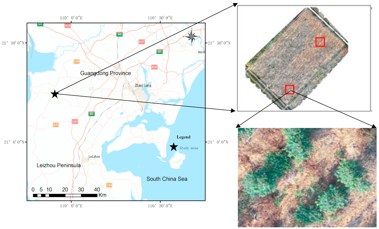
2.1. Study Area and Datasets

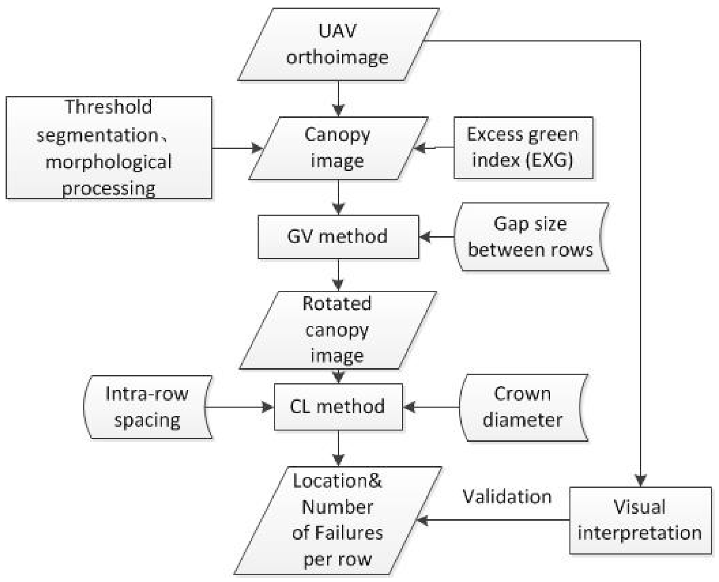
This study area is located in a Eucalyptus forestry site of Leizhou Peninsula, Guangdong Province, Southern China (20°16′38.5″N, 109°56′44.7″E). The Eucalyptus forestry site is located at the northern edge of tropics, which has a maritime monsoon climate with annual temperatures of 21–26 °C and annual precipitations of 1300–2500 mm. The study area is a pure forest of Eucalyptus, with sparse understory vegetation and trees distributed in rows with a 3 m spacing between rows and a 1.5 m spacing between plants within rows.

A light UAV, DJI Genie 4, was used to acquire high-resolution visible-light images of the study area. The UAV was equipped with a visible-light camera with 20 megapixels and an equivalent focal length of 24 mm. Images were taken at noon on 15 November 2019, with an 80% overlap in the heading direction and a 75% overlap in the side direction. The weather was sunny with no wind, the terrain was flat, the flight altitude was 100 m, and the photo resolution was 5472 × 3648 pixels. A total of 316 images were acquired. The Pix4D mapper software was used to stitch adjacent images to generate orthoimages with a ground resolution of 1 cm. The acquired orthoimage and the locations of the two test areas intercepted in this study are shown in Figure 1.

2.2. Methodology

The outline of the proposed methodology is shown in Figure 2. It involves two key technical methods: the GV method to interpret the direction angle of seedling rows and the CL method to find the relative locations and the number of failures in each row.

All analyses about the two intercepted images were implemented in MATLAB including vegetation index calculation, threshold segmentation, morphological processing, and GV method and CL method calculations.

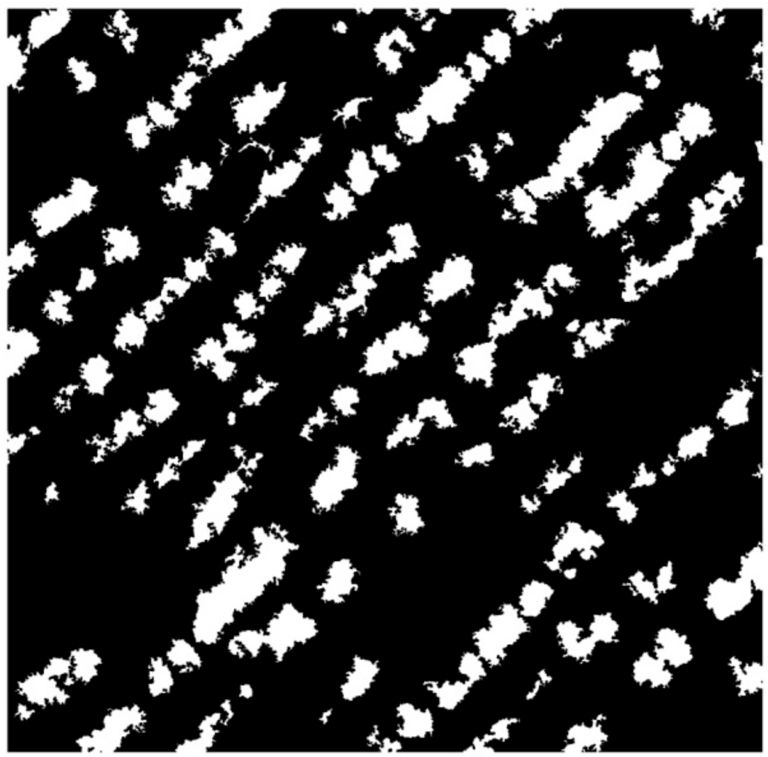
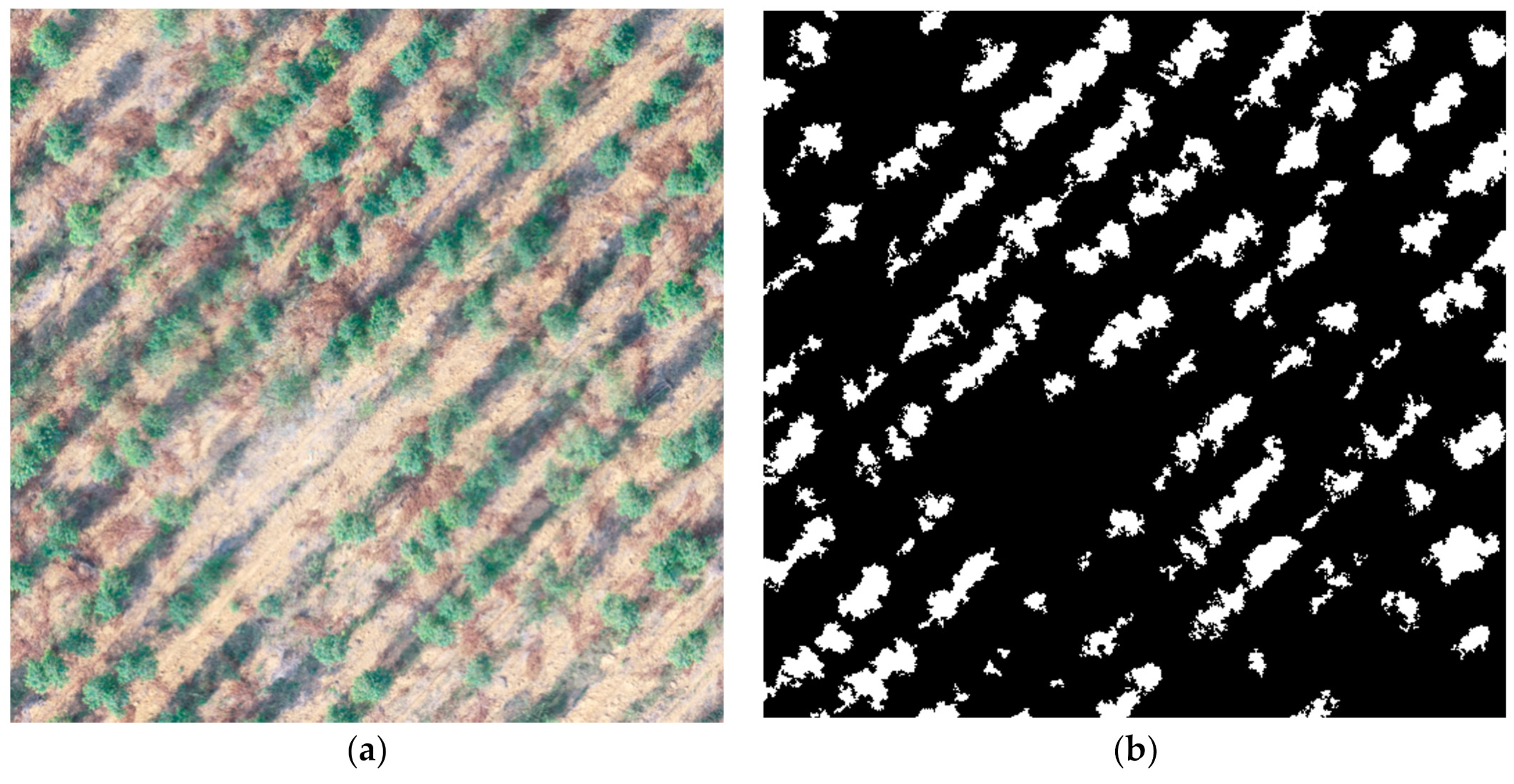
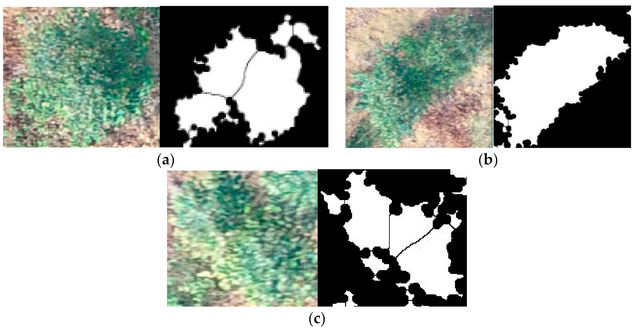
2.2.1. Seedling Recognition

Firstly, in order to distinguish the green canopy from other backgrounds, such as shadows, soil, and stones, the vegetation index (Equation (1)) proposed by Søgaard and Olsen was used to extract green pixels [44]:

EXG = 2G − R − B,

(1)

where R, G, and B, are the pixel values in red, green, and blue light bands, respectively.

There is a small amount of grass of which the spectral characteristics are very similar to those of canopy in the study area, and distinguishing them from canopy is beyond the discussion of this paper.

Secondly, Otsu’s method [44] was applied to obtain the binary images of the test areas. Ostu’s method is one of the best methods to determine threshold [20].

Finally, morphological processing was performed on the image: close operations and hole filling were used to obtain continuous and smooth crown, and small areas were removed as their area was too small to be treated as crown.

The result is shown in Figure 3.

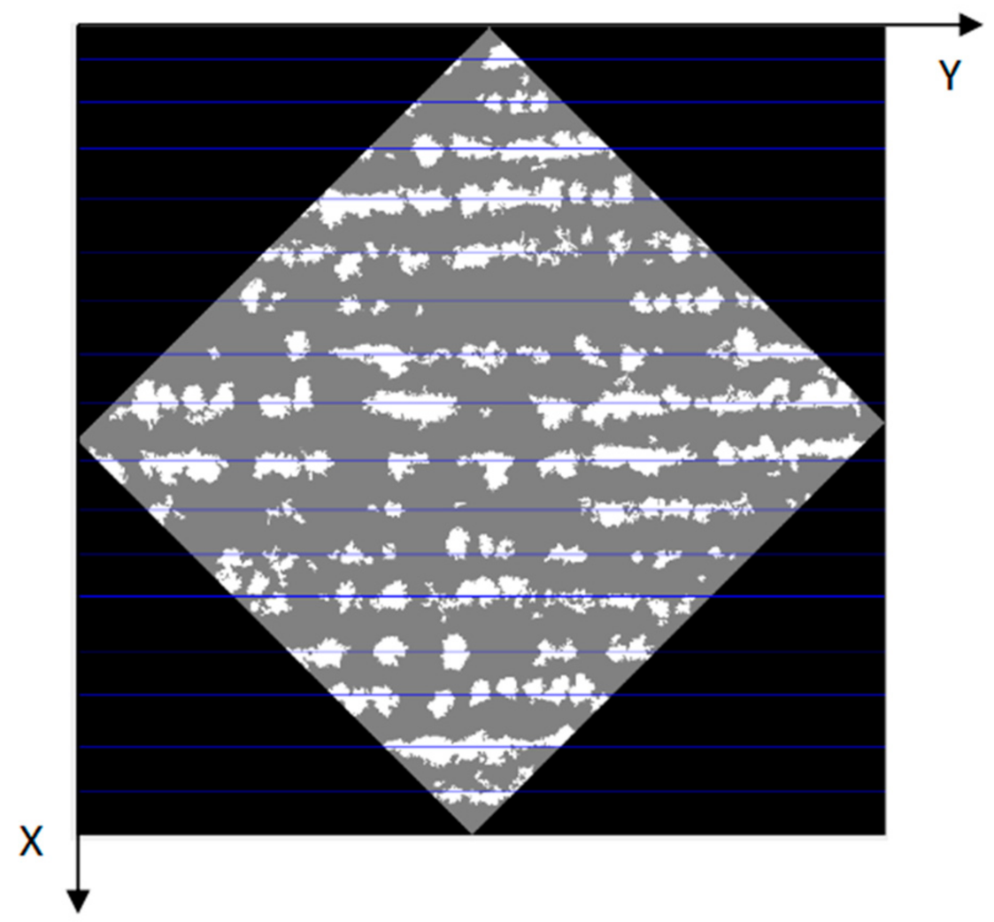
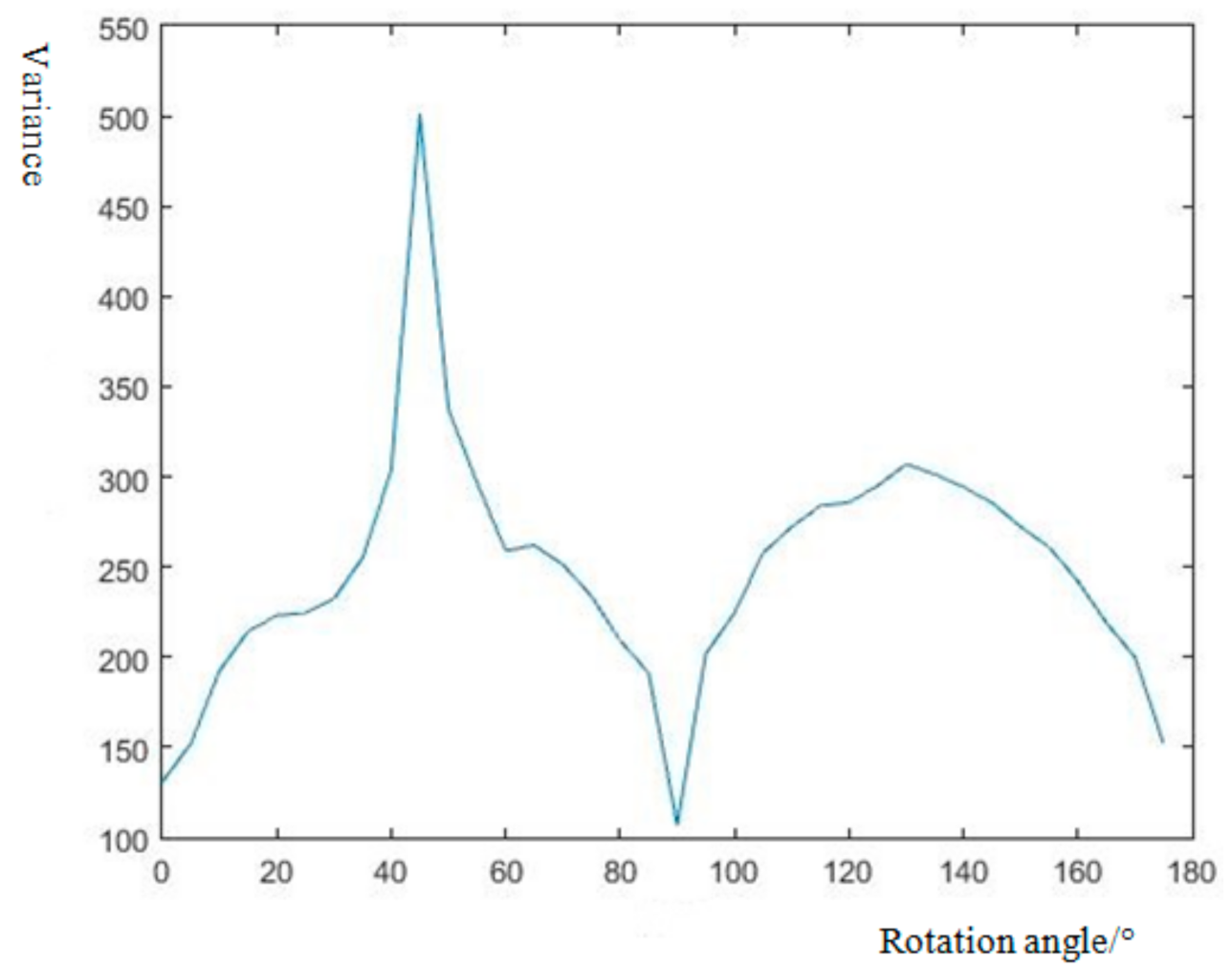
2.2.2. Interpretation of the Direction Angle of Seedling Rows in the Orthoimage by the GV Method

In order to subsequently determine the relative positions of the failures in rows, we needed to determine the orientation of the seedling row which is not always parallel with the horizontal axis or vertical axis (in this study, we chose the horizontal axis as the reference line) and then rotate them to a horizontal position.

Given that in the orthoimage, the seedlings were orderly distributed in rows rather than evenly throughout the whole area, there was a set of horizontal grids (the number of grids was denoted as Num) was assumed parallel to each other covering the whole image. If the binary image was rotated to different angles, the canopy pixels were distributed differently within the grids. When the direction of seedling rows was parallel to the horizontal grid lines (Y-axis), if the width of each grid was smaller than the width of the gap between rows, then an extreme distribution occurred, that is, there were many canopy pixels in some of the grids while a little or even none canopy pixels were in other grids. In other words, the distribution of canopy pixels within the grids was extremely uneven throughout the orthoimage. Based on the distribution of canopy pixels in the horizontal grid, we can use the sample variance of the sequence of the number of canopy pixels in each grid (the number of canopy pixels in each grid was denoted as ${\mathrm{N}}_{\mathrm{i}}$, and the average number of canopy pixels in each grid was represented by $\overline{\mathrm{N}}$) to measure the degree of uniformity of the canopy pixels distribution. The sample variance (S²) was calculated as:

$${\mathrm{S}}^2=\frac{{{\displaystyle \sum }}_1^{\mathrm{Num}}{\left({\mathrm{N}}_{\mathrm{i}}-\overline{\mathrm{N}}\right)}^2}{\mathrm{Num}-1}.$$

(2)

It was assumed that the original image was rotated clockwise from 0° to 180° (e.g., in steps of Δ = 5°), and the sample variance ${\mathrm{S}}_{\mathrm{j}}\left({\mathsf{\beta }}_{\mathrm{j}}\right)$ of the canopy pixels distribution was recorded corresponding to each rotation angle ${\mathsf{\beta }}_{\mathrm{j}}$. The rotation angle ${\mathsf{\beta }}_{\mathrm{k}}$ corresponding to the maximum sample variance $\max \left({\mathrm{S}}_{\mathrm{j}}\left({\mathsf{\beta }}_{\mathrm{j}}\right)\right)$ was direction angle ${\mathsf{\beta }}_0$ of seedling rows, which can be written as:

$${\mathsf{\beta }}_0={\mathsf{\beta }}_{\mathrm{k}}{ \mathrm{if} \mathrm{S}}_{\mathrm{k}}\left({\mathsf{\beta }}_{\mathrm{k}}\right)=\max \left({\mathrm{S}}_{\mathrm{j}}\left({\mathsf{\beta }}_{\mathrm{j}}\right)\right) \left\{\mathrm{j}=1,2,3\dots \frac{{180}^{°}}{∆}\right\},$$

(3)

where j denotes the jth rotation.

A diagram of the principle of the GV method is shown in Figure 4.

The algorithm of the GV method is presented as follows.

Step 1: Rotate the image clockwise by angle θ.

Step 2: Gridding: the maximum X-coordinate and the minimum X-coordinate (the unit is pixel) of the canopy are calculated, and then, the interval [Xmin, Xmax] is divided into a horizontal grid with interval L. The number of subintervals is Num, i.e., [Xmin, Xmin + L), [Xmin + L, Xmin + 2L] …, [Xmin + (Num − 1) × L, Xmax].

Step 3: Count the number of canopy pixels falling into each horizontal grid in step 2, $N_i$, and calculate the sample variance S²_j, with subscript j indicating the jth rotation of the image.

Step 4: Repeat steps 1 to 3 until the image is rotated 180° to obtain the sample variance S² of the canopy pixels distribution in different directions, and the rotation angle corresponding to the maximum variance is the direction angle of the seedling rows.

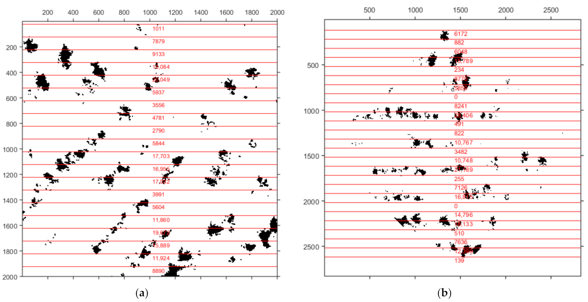
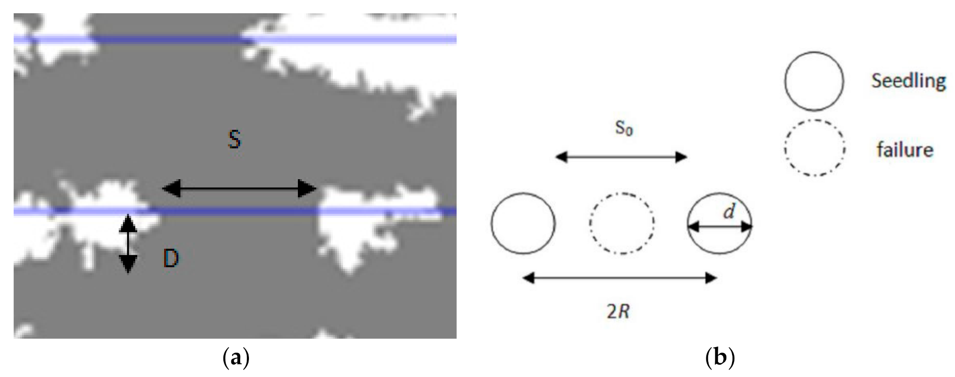
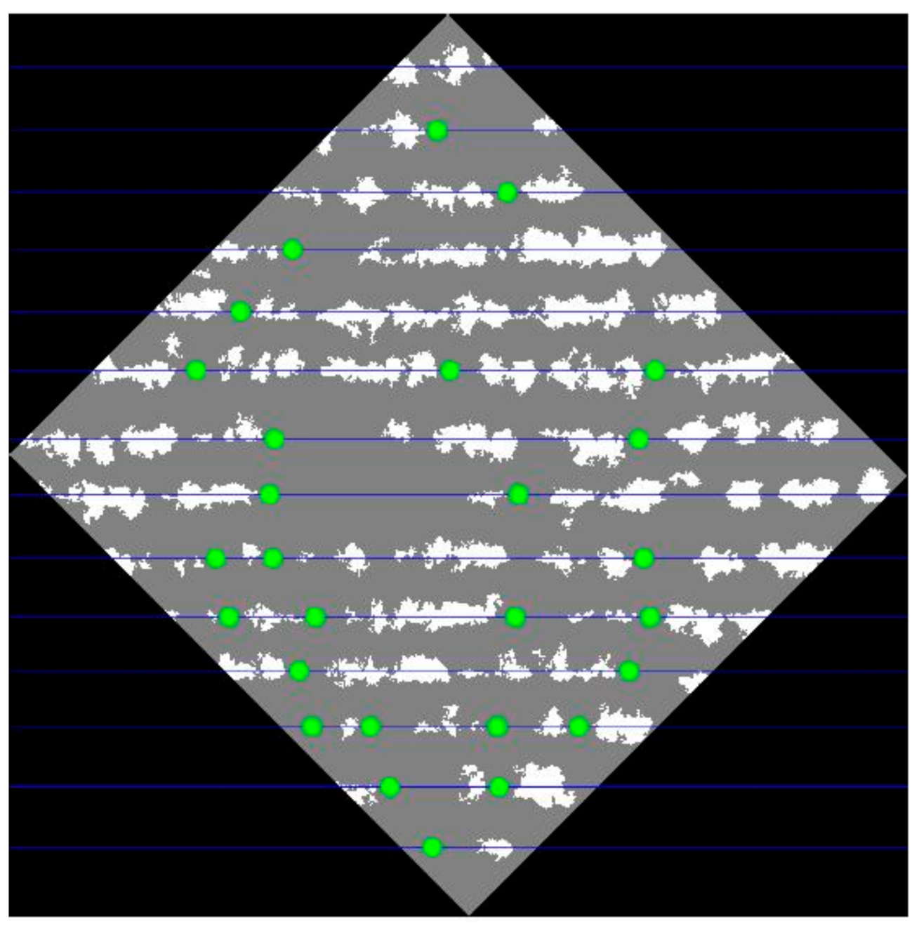
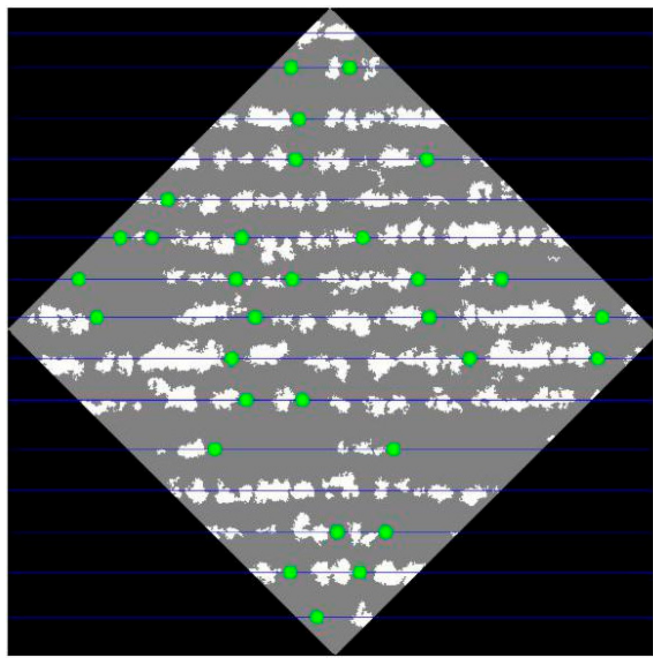
2.2.3. Detection of Failures and Interpretation of Their Relative Locations in Rows

Direction angle ${\mathsf{\beta }}_0$ was calculated by the GV method, and the original canopy image was rotated clockwise by angle ${\mathsf{\beta }}_0$ so that the seedling rows were in a horizontal position.

When seedlings were distributed horizontally in rows, we obtained the centerlines of all seedling rows. The presence or absence of canopy pixels near the centerline of each row was directly related to the failures in that row. Combining the information about the spacing between rows and spacing within rows, we proposed a method (CL method) to detect failures and collect their relative locations and numbers in each row.

The algorithm of the CL method is presented as follows:

Step 1: Rotate an original image to the horizontal position, as shown in Figure 5. As the seedling rows are all horizontal, if canopy pixels in each row are projected onto the X-axis, we will see that the projected pixel points are clustered and spaced on the X-axis because of the large gap between two adjacent seedling rows.

Step 2: Use K-means clustering to obtain the respective center point of each cluster of the projected points on the X-axis [45]. Obviously, the number of clusters is the total number of seedlings rows in the image.

Step 3: Find the relative locations and number of the failures along each centerline using the CL method.

The detailed process of the CL method is shown as following: Firstly, horizontal and parallel centerlines are drawn through each center point, as shown in Figure 5. Secondly, for each pixel on the centerline (denoted as point p), the number of non-vegetated pixels among pixels is found, which is above or below p and less than D (i.e., half the average diameter) pixels away from p. If none of the pixels are vegetated, point p is considered to be non-vegetated, otherwise it is considered to be vegetated. If the length of successive non-vegetated pixels S (shown in Figure 6a) reaches a certain threshold value S₀ (shown in Figure 6b and Equation (5)), i.e., $\mathrm{S}>{\mathrm{S}}_0$, failure occurs, and we define the starting location of the successive failures (successive non-vegetated pixels of which the length is longer than S₀) as the relative location. The relative location was denoted as (Rn, Dn), where Rn is the number of the row and Dn represents the departure from the starting. Thirdly, the number of failures N_i in this row was counted as:

$${\mathrm{N}}_{\mathrm{i}}={{\displaystyle \sum }}_{\mathrm{j}=1}^{\mathrm{n}}\left[\frac{{\mathrm{S}}_{\mathrm{j}}+\mathsf{\delta }}{\mathrm{R}}\right],$$

(4)

$${\mathrm{S}}_0=2\mathrm{R}-\mathrm{d},$$

(5)

$$\mathsf{\delta }=\mathrm{R}-{\mathrm{S}}_0,$$

(6)

where Si, R, and d are the length of the jth successive failures in this line, the spacing within rows, and the maximum diameter of trees, respectively.

In Equation (4), the numerator is ${\mathrm{S}}_{\mathrm{j}}+\mathsf{\delta }$ instead of ${\mathrm{S}}_{\mathrm{j}}$, this is because we treated S, which reaches ${\mathrm{S}}_0$ but does not reach R, as a failure.

3. Results and Discussion

The parameters involved in the experiment were shown as following: R = 1.5 m, i.e., 145 pixels on an image, and the maximum canopy diameter d = 1.8 m, i.e., 174 pixels by the statistics of the canopy size. S₀ = 116 pixels in size. The size of L was a figure smaller than the width of the gap between rows (denoted as G). Here, we set L to be 0.6G, i.e., 168 pixels.

The RGB image and the binary image of canopy of test area 1 (Test_1) are shown in Figure 7. The result (Figure 8) showed the distribution of the variance of the GV method, and there was a distinct peak in variance curve at the rotation angle of 45° that was the direction angle of Test_1. During the calculation, in order to avoid the variance to be too big, the weight of each pixel was set to 0.01. The relative locations on the map of the detected successive failures in Test_1 are shown in Figure 9. The failure information of Test_1 is shown in

Table 2. Failure information of Test_1.

Rn 1 (N 2)	Dn 3/m (PN 4)
1(0)	No failure
2(3)	4.8(3)
3(1)	11.4(1)
4(2)	3.5(2)
5(1)	3.8(1)
6(3)	4.6(1) 17.6(1) 28(1)
7(5)	12.1(4) 30.6(1)
8(8)	10.6(7) 23.3(1)
9(4)	4.6(1) 7.6(1) 26.4(2)
10(5)	2.4(1) 6.7(1) 16.8(2) 23.7(1)
11(3)	3.2(1) 20.0(2)
12(5)	1.0(1) 4.1(1) 10.5(2) 14.6(1)
13(3)	2.0(2) 7.5(1)
14(2)	1.0(2)

¹ Row number. ² Number of failures in row Rn. ³ Each successive failures’ departure from the starting point of row Rn. ⁴ Number of failures each successive failures contain.

, which included the row number (denoted as Rn), the total number of failures in this row (denoted as N), each successive failures’ departure from the starting point of this row (denoted as Dn), and the number of failures the successive failures contain (denoted as PN). The overall detection rate of failures was 91.8% (Table 4).

The relative locations of the successive failures in test area 2 (Test_2) are shown in Figure 10. The failure information of Test_2 is shown in

Table 3. Failure information of Test_2.

Rn 1 (N 2)	Dn 3/m (PN 4)
1(0)	No failure
2(3)	1.0(2) 5.3(1)
3(1)	5.4(1)
4(3)	8.1(1) 17.8(2)
5(1)	1.7(1)
6(4)	1.0(1) 3.4(1) 10.0(1) 18.9(1)
7(12)	1.0(4) 12.6(1) 16.7(1) 26.0(2) 32.0(4)
8(7)	5.1(4) 16.8(1) 29.6(1) 42.3(1)
9(3)	13.8(1) 31.3(1) 40.7(1)
10(2)	11.8(1) 15.9(1)
11(13)	5.9(6) 19.0(7)
12(0)	No failure
13(4)	8.8(1) 12.3(3)
14(2)	1.8(1) 7.0(1)
15(2)	1.0(2)

¹ Row number. ² Number of failures in row Rn. ³ Each successive failures’ departure from the starting point of row Rn. ⁴ Number of failures each successive failures contain.

. The overall detection rate of Test_2 was 95% (

Table 4. Overall detection rates of Test_1 and Test_2.

Test Area	Number of Failures (Proposed Method)	Number of Failures (Visual Interpretation)	Overall Detection Rate
Test_1	45	49	91.8%
Test_2	57	60	95%

).

Although the detection rates of failures were above 90% for the two sample areas, the detection rate of failures was underestimated. The reason is as following: to a great extent, it depends on the accuracy of the distinction between the canopy and the background. In the study areas randomly selected from Eucalyptus forests, some failures were not detected, because there were many weeds growing there of which the spectral characteristics were similar to the canopy. The weeds can easily be misclassified as canopy. In this study, we cared more about the relative failures positions than their detection rates. Thus, the distinction between Eucalyptus canopy from weeds was not studied here.

For the researches on the detection rate of failures, to the best of the author’s knowledge, most researchers concentrated on extracting individual trees and counting the number. If the trees are distributed regularly, then number of failures can be inferred by the number of trees detected. In our study, we compared the experimental results from the proposed method with that with the watershed method, which is widely used by researchers to derive the individual trees [46,47]. Based on the same test data (the binary images of Test_1 and Test_2 obtained in Section 2.2.1), watershed image segmentation was conducted in the ImageJ software.

Most of the linked canopies in the images were segmented, and the number of the detected crown was denoted as ${\mathrm{N}}_{\mathrm{real}}$. As the Eucalyptus in the study area were planted at a basic fixed row spacing and intra-row spacing, the theoretical number of plants that could be accommodated by Test_1 and Test_2 can be obtained from Equation (7):

$${\mathrm{N}}_{\mathrm{tree}-\mathrm{total}}=\frac{\mathrm{S}}{\mathrm{R}\times \mathrm{K}},$$

(7)

where ${\mathrm{N}}_{\mathrm{tree}-\mathrm{total}}$ is the number of trees the test area can hold; S is the area of Test_1 or Test_2; R is the intra-row spacing; K is the row spacing.

Thus, the number of failures can be obtained by subtracting ${\mathrm{N}}_{\mathrm{real}}$ form ${\mathrm{N}}_{\mathrm{tree}-\mathrm{total}}$. The overall detection rates of failures in Test_1 and Test_2 were 55% and 63%, respectively, which were both lower than those using CL method. This is because the CL method is dependent on how well the canopy is separated from the background and does not rely on the results of the canopy-to-canopy segmentation. The number of failures obtained using the watershed method depends not only on the degree of separation between canopy and background, but also on the effectiveness of the canopy-to-canopy segmentation, while the watershed method has the phenomenon of over-segmentation (Figure 11a) and under-segmentation (Figure 11b), resulting in inaccurate segmentation numbers. In addition, the distribution of Eucalypts is not absolutely uniform, so there are some errors in calculating the total number of plants based on the row spacing, intra-row spacing, and total area. Another very important factor affecting the accuracy of the watershed method in obtaining failures is that the study area is a Eucalyptus sprouting forest and it is common to have two seedlings growing from one stump (Figure 11c), which is commonly identified by the watershed method as two or more trees but only occupies the space of one tree. In addition, even though watershed segmentation allows for an accurate number of failures to be obtained, the exact locations and the corresponding number of failures are not available.

Compared with the geographic coordinates provided by the images, the advantage of the relative locations of the failures expressed by row numbers proposed in this paper is as following: The row spacing in Eucalyptus plantations is usually much wider than the intra-row spacing in order to facilitate mechanical inter-row operations. For example, the row spacing in the test area is 3 m, and the intra-row spacing is 1.5 m. When looking for the corresponding location according to geographical coordinates, it is necessary to shuttle through the forest, and this shuttle may exist in any direction, perhaps along a certain row or between rows, which is not convenient for foresters to find or for mechanical equipment to operate. However, if the row position of the failure location is known, it is easier for the mechanical equipment to find the failure location along a certain row direction according to the row number.

4. Conclusions

In this paper, a method of failure detection in young Eucalyptus forests was proposed. Based on tests, we can see that the proposed methodology is feasible and can be used for the automatic calculation of the failure rate and the efficient guidance of replanting. The proposed GV method can be used to calculate the direction angle of seedling rows correctly, where trees are arranged in regular rows. The CL method can correctly obtain the locations and the number of failures in each row. From the experimental results, results with an acceptable accuracy were obtained with the proposed methodology (detection rate of failures: >90%), which can be improved by a more intensive study to distinguish weeds from tree canopy. Thus, as a future work, the authors will focus more on image feature analysis and aim to distinguish tree canopy from other vegetation in order to better extract tree canopy and detect failures more accurately.

References

1. Dash, J.; Pont, D.; Brownlie, R.; Dunningham, A.; Watt, M.S. Remote sensing for precision forestry. N. Z. J. For. 2016, 60, 15–24. [Google Scholar]
2. Choudhry, H.; O’Kelly, G. Precision forestry: A revolution in the woods. McKinsey Insights 2018, 1. [Google Scholar]
3. PR Newswire. US Global Precision Market Projected to Reach $6.1 Billion by 2024, at a CAGR of 9% during 2019–2024; PR Newswire: New York, NY, USA, 2019. [Google Scholar]
4. Mohan, M.; Silva, C.A.; Klauberg, C.; Jat, P.; Catts, G.; Cardil, A.; Hudak, A.T.; Dia, M. Individual tree detection from unmanned aerial vehicle (UAV) derived canopy height model in an open canopy mixed conifer forest. Forests 2017, 8, 340. [Google Scholar] [CrossRef] [Green Version]
5. Dai, W.; Yang, B.; Dong, Z.; Shaker, A. A new method for 3D individual tree extraction using multispectral airborne LiDAR point clouds. ISPRS J. Photogramm. Remote Sens. 2018, 144, 400–411. [Google Scholar] [CrossRef]
6. Mu, Y.; Fujii, Y.; Takata, D.; Zheng, B.Y.; Noshita, K.; Honda, K.; Ninomiya, S.; Guo, W. Characterization of peach tree crown by using high-resolution images from an unmanned aerial vehicle. Hortic. Res. 2018, 5, 74. [Google Scholar] [CrossRef] [PubMed] [Green Version]
7. Peuhkurinen, J.; Tokola, T.; Plevak, K.; Sirparanta, S.; Kedrov, A.; Pyankov, S. Predicting tree diameter distributions from airborne laser scanning, SPOT 5 satellite, and field sample data in the Perm Region, Russia. Forests 2018, 9, 639. [Google Scholar] [CrossRef] [Green Version]
8. Ganz, S.; Käber, Y.; Adler, P. Measuring tree height with remote sensing-a comparison of photogrammetric and LiDAR data with different field measurements. Forests 2019, 10, 694. [Google Scholar] [CrossRef] [Green Version]
9. Wu, J.; Yang, G.; Yang, H.; Zhu, Y.; Li, Z.; Lei, L.; Zhao, C. Extracting apple tree crown information from remote imagery using deep learning. Comput. Electron. Agr. 2020, 174, 105504. [Google Scholar] [CrossRef]
10. Wulder, M.A.; White, J.C.; Nelson, R.F.; Nsset, E.; Rka, H.O.; Coops, N.C.; Hilker, T.; Bater, C.W.; Gobakken, T. Lidar sampling for large-area forest characterization: A review. Rem. Sens. Environ. 2012, 121, 196–209. [Google Scholar] [CrossRef] [Green Version]
11. Penner, M.; Woods, M.; Pitt, D.G. A Comparison of Airborne Laser Scanning and Image Point Cloud Derived Tree Size Class Distribution Models in Boreal Ontario. Forests 2015, 6, 4034–4054. [Google Scholar] [CrossRef] [Green Version]
12. Díaz-Varela, R.A.; de la Rosa, R.; León, L.; Zarco-Tejada, P.J. High-Resolution Airborne UAV Imagery to Assess Olive Tree Crown Parameters Using 3D Photo Reconstruction: Application in Breeding Trials. Remote Sens. 2015, 7, 4213–4232. [Google Scholar] [CrossRef] [Green Version]
13. Moe, K.T.; Owari, T.; Furuya, N.; Hiroshima, T. Comparing Individual Tree Height Information Derived from Field Surveys, LiDAR and UAV-DAP for High-Value Timber Species in Northern Japan. Forests 2020, 11, 223. [Google Scholar] [CrossRef] [Green Version]
14. Dandois, J.P.; Ellis, E.C. High Spatial Resolution Three-Dimensional Mapping of Vegetation Spectral Dynamics Using Computer Vision. Rem. Sens. Environ. 2013, 136, 259–276. [Google Scholar] [CrossRef] [Green Version]
15. Guerra-Hernández, J.; Cosenza, D.N.; Rodriguez, L.C.E.; Silva, M.; Tome, M.; Di´az-Varela, R.A.; Gonza´lez-Ferreiro, E. Comparison of ALS- and UAV(SfM)-derived high-density point clouds for individual tree detection in Eucalyptus plantations. Int. J. Remote Sens. 2018, 39, 5211–5235. [Google Scholar] [CrossRef]
16. Barawid, O.C.; Mizushima, A.; Ishii, K.; Noguchi, N. Development of an autonomous navigation system using a two-dimensional laser scanner in an orchard application. Biosyst. Eng. 2007, 96, 139–149. [Google Scholar] [CrossRef]
17. Jiang, G.; Wang, X.; Wang, Z. Wheat rows detection at the early growth stage based on Hough transform and vanishing point. Comput. Electron. Agric. 2016, 123, 211–223. [Google Scholar] [CrossRef]
18. Montalvo, M.; Pajares, G.; Guerrero, J.M.; Romeo, J.; Guijarro, M.; Ribeiro, A.; Ruz, J.J.; Cruz, J.M. Automatic detection of crop rows in maize fields with high weeds pressure. Expert Syst. Appl. 2012, 39, 11889–11897. [Google Scholar] [CrossRef] [Green Version]
19. Choi, K.H.; Han, S.K.; Han, S.H.; Park, K.-H.; Kim, K.-S.; Kim, S. Morphology-based guidance line extraction for an autonomous weeding robot in paddy fields. Comput. Electron. Agric. 2015, 113, 266–274. [Google Scholar] [CrossRef]
20. Jiang, G.; Wang, Z.; Liu, H. Automatic detection of crop rows based on multi-ROIs. Expert Syst. Appl. 2015, 42, 2429–2441. [Google Scholar] [CrossRef]
21. Fontaine, V.; Crowe, T.G. Development of line-detection algorithms for local positioning in densely seeded crops. Can. Biosyst. Eng. 2006, 48, 19. [Google Scholar]
22. Kise, M.; Zhang, Q. Development of a stereovision sensing system for 3D crop row structure mapping and tractor guidance. Biosyst. Eng. 2008, 101, 191–198. [Google Scholar] [CrossRef]
23. Vidović, I.; Scitovski, R. Center-based clustering for line detection and application to crop rows detection. Comput. Electron. Agr. 2014, 109, 212–220. [Google Scholar] [CrossRef]
24. Zhang, X.; Li, X.; Zhang, B. Automated robust crop-row detection in maize fields based on position clustering algorithm and shortest path method. Comput. Electron. Agr. 2018, 154, 165–175. [Google Scholar] [CrossRef]
25. Vidović, I.; Cupec, R.; Hocenski, Ž. Crop Row Detection by Global Energy Minimization. Pattern Recogn. 2016, 55, 68–86. [Google Scholar] [CrossRef]
26. Tenhunen, H.; Pahikkala, T.; Nevalainen, O.; Teuhola, J.; Mattila, H.; Tyystjärvi, E. Automatic detection of cereal rows by means of pattern recognition techniques. Comput. Electron. Agr. 2019, 162, 677–688. [Google Scholar] [CrossRef]
27. García-Santillín, I.; Guerrero, J.M.; Montalvo, M.; Pajares, G. Curved and straight crop row detection by accumulation of green pixels from images in maize fields. Precis. Agric. 2018, 19, 18–41. [Google Scholar] [CrossRef]
28. Oliveira, H.C.; Guizilini, V.C.; Nunes, I.P.; Souza, J.R. Failure detection in row crops from UAV images using morphological operators. IEEE Geosci. Remote Sens. 2018, 15, 991–995. [Google Scholar] [CrossRef]
29. Li, B.; Xu, X.; Han, J.; Zhang, L.; Bian, C.; Jin, L.; Liu, J. The estimation of crop emergence in potatoes by UAV RGB imagery. Plant Methods 2019, 15, 15. [Google Scholar] [CrossRef] [PubMed] [Green Version]
30. Dai, J.; Xue, J.; Zhao, Q.; Wang, Q.; Chen, B.; Zhang, G.; Jiang, N. Extraction of cotton seedling growth information using UAV visible light remote sensing images. Trans. CSAE 2020, 36, 63–71. [Google Scholar] [CrossRef]
31. Jin, X.; Liu, S.; Baret, F.; Hemerlé, M.; Comar, A. Estimates of plant density of wheat crops at emergence from very low altitude UAV imagery. Remote Sen. Environ. 2017, 198, 105–114. [Google Scholar] [CrossRef] [Green Version]
32. Shirzadifar, A.; Maharlooei, M.; Bajwa, S.G.; Oduor, P.G.; Nowatzki, J.F. Mapping crop stand count and planting uniformity using high resolution imagery in a maize crop. Biosyst. Eng. 2020, 200, 377–390. [Google Scholar] [CrossRef]
33. Kestur, R.; Angural, A.; Bashir, B.; Omkar, S.N.; Anand, G.; Meenavathi, M.B. Tree crown detection, delineation and counting in UAV remote sensed Images: A neural network based spectral–spatial Method. J. Indian Soc. Remote 2018, 46, 991–1004. [Google Scholar] [CrossRef]
34. Ampatzidis, Y.; Partel, V. UAV-based high throughput phenotyping in citrus utilizing multispectral imaging and artificial intelligence. Remote Sens. 2019, 11, 410. [Google Scholar] [CrossRef] [Green Version]
35. Csillik, O.; Cherbini, J.; Johnson, R.; Lyons, A.; Kelly, M. Identification of citrus trees from unmanned aerial vehicle imagery using convolutional neural networks. Drones 2018, 2, 39. [Google Scholar] [CrossRef] [Green Version]
36. Zhou, J.; Proisy, C.; Descombes, X.; Maire, G.L.; Nouvellon, Y.; Stape, J.-L.; Viennois, G.; Zerubia, J.; Couteron, P. Mapping local density of young Eucalyptus plantations by individual tree detection in high spatial resolution satellite images. For. Ecol. Manage. 2013, 301, 129–141. [Google Scholar] [CrossRef] [Green Version]
37. Li, W.; Fu, H.; Yu, L.; Cracknell, A. Deep learning based oil palm tree detection and counting for high-resolution remote sensing images. Remote Sens. 2017, 9, 22. [Google Scholar] [CrossRef] [Green Version]
38. Zheng, J.; Fu, H.; Li, W.; Wu, W.; Zhao, Y.I.; Dong, R.; Yu, L.E. Cross-regional oil palm tree counting and detection via a multi-level attention domain adaptation network. ISPRS J. Photogramm. Remote Sens. 2020, 167, 154–177. [Google Scholar] [CrossRef]
39. Shi, Y.; Wang, N.; Taylor, R.K.; Raun, W.R. Improvement of a ground-LiDAR-based corn plant population and spacing measurement system. Comput. Electron. Agr. 2015, 112, 92–101. [Google Scholar] [CrossRef]
40. Tai, Y.W.; Ling, P.P.; Ting, K.C. Machine vision assisted robotic seedling transplanting. Trans. ASABE 1994, 37, 661–667. [Google Scholar] [CrossRef]
41. Ryu, K.H.; Kim, G.; Han, J.S. Development of a robotic transplanter for bedding plants. J. Agr. Eng. Res. 2001, 78, 141–146. [Google Scholar] [CrossRef]
42. Wang, C.; Guo, X.; Xiao, B.; Du, J.; Wu, S. Automatic measurement of numbers of maize seedlings based on mosaic imaging. Trans. CSAE 2014, 30, 148–153. [Google Scholar] [CrossRef]
43. Molin, J.P.; Veiga, J.P.S. Spatial variability of sugarcane row gaps: Measurement and mapping. Ciência Agrotecnologia 2016, 40, 347–355. [Google Scholar] [CrossRef] [Green Version]
44. Otsu, N. A threshold selection method from gray-level histograms. Automatica 1975, 11, 285–296. [Google Scholar] [CrossRef] [Green Version]
45. MacQueen, J. Some Methods for Classification and Analysis of Multivariate Observation; University of California Press: Berkeley, CA, USA, 1967; pp. 281–297. [Google Scholar]
46. Girish Kumar, D.; Raju, C.; Harish, G. Individual tree crowns computation using watershed segmentation in urban environment (Article). J. Green Eng. 2020, 10, 2644–2660. [Google Scholar]
47. Huang, H.Y.; Li, X.; Chen, C.C. Individual tree crown detection and delineation from very high resolution UAV images based on bias field and Marker-Controlled Watershed segmentation algotithms. IEEE J. Sel. Top. Appl. Earth Obs. Remote Sens. 2018, 11, 2253–2262. [Google Scholar] [CrossRef]
Figure 1. The orthoimages and the locations of two test areas.
Forests 12 01250 g001
Figure 2. Outline of the methodology.
Forests 12 01250 g002
Figure 3. Binary image (canopy image). The tree crowns are indicated in white, and the background is indicated in black.
Forests 12 01250 g003
Figure 4. The diagram of the grid-variance (GV) method: (a) distribution of canopy pixels in grids before rotation; (b) distribution of canopy pixels in grids after rotation. Note: the figure in red is the number of canopy pixels in each grid.
Forests 12 01250 g004
Figure 5. Diagram of the centerlines (in blue) of the seedling rows.
Forests 12 01250 g005
Figure 6. Schematic diagrams for the detection of failures: (a) detection of failures; (b) threshold S0.
Forests 12 01250 g006
Figure 7. RGB image and canopy image of Test_1: (a) RGB image; (b) binary image of canopy.
Forests 12 01250 g007
Figure 8. Distribution of S2 with L = 0.6 G.
Forests 12 01250 g008
Figure 9. Relative locations (green dots) of the successive failures in Test_1 (Blue lines: centerlines of seedling rows).
Forests 12 01250 g009
Figure 10. The relative locations (green dots) of the successive failures in Test_2 (Blue lines: centerlines of seedling rows).
Forests 12 01250 g010
Figure 11. The results of incorrect segmentation obtained with the watershed method: (a) over-segmentation; (b) under-segmentation; (c) two seedlings from one stump.
Forests 12 01250 g011