Revisiting the Performance of the Kernel-Driven BRDF Model Using Filtered High-Quality POLDER Observations

Abstract

The Bidirectional Reflectance Distribution Function (BRDF) is usually used to describe the reflectance anisotropy of a non-Lambertian surface and estimate surface parameters. Among the BRDF models, the kernel-driven models have been extensively used due to their simple form and powerful fitting ability, and their reliability has been validated in some studies. However, existing validation efforts used in situ measurements or limited satellite data, which may be subject to inadequate observational conditions or quality uncertainties. A recently released high-quality BRDF database from Polarization and Directionality of the Earth’s Reflectances (POLDER) provides an opportunity to revisit the performance of the kernel-driven models. Therefore, in order to evaluate the fitting ability of the kernel-driven models under different observational conditions and explore their application direction in the future, we use the filtered high-quality BRDF database to evaluate the fitting ability of the kernel-driven model represented by the RossThick-LiSparseR (RTLSR) kernels in this paper. The results show that the RTLSR model performs well, which shows small fitting residuals under most observational conditions. However, the applicability of the RTLSR model performed differently across land cover types; the RTLSR model exhibited larger fitting residuals, especially over non-vegetated surfaces. Under different sun-sensor geometries, the fitting residuals show a strong positive correlation with the Solar Zenith Angle. The above two factors cause the RTLSR model to exhibit a poorer fitting ability at high latitudes. As an exploration, we designed a model combination strategy that combines the advantages of different models and achieved a better performance at high latitudes. We believe that this study provides a better understanding of the RTLSR model.

1. Introduction

The Bidirectional Reflectance Distribution Function (BRDF) is defined as the ratio of the radiance in the direction of the exit beam to the irradiance caused by the entrance beam [1]. In remote sensing, BRDF commonly represents the distribution of bidirectional reflectance to quantify surface reflectance anisotropy [2]. An accurate estimate of land surface BRDF serves to correct the bidirectional effects in vegetation indices and reflectance and to estimate land surface physical, biological parameters, and vegetation structural parameters, such as albedo and leaf area index (LAI) from reflectance measurements [3,4,5,6,7]. Therefore, accurate modeling of the global land surface BRDF is important for global ecosystem monitoring and radiation balance researches.

Several empirical, semi-empirical, and physical methods have been developed for BRDF modeling. Among them, the semi-empirical linear kernel-driven models introduced by Roujean et al. [8] have been widely used. Wanner et al. [9] and Lucht et al. [6] subsequently improved the kernel-driven model to make it easier to understand and apply as the Algorithm for Model Bidirectional Reflectance Anisotropies of the Land Surface (AMBRALS) [10]. The kernel-driven models were adopted as the operational algorithms for generating land surface albedo products by many spaceborne sensors, including the Moderate Resolution Imaging Spectroradiometer (MODIS) and Polarization and Directionality of the Earth’s Reflectances (POLDER) [6,11,12,13,14,15,16]. Scholars developed many kernels to describe the radiative transfer process of different scenes, such as the well-known Ross kernels and Li kernels [6,8,17]. Li et al. [17,18] also developed a kernel called the LiTransit kernel to describe the geometric–optical relationships of discrete canopies under large zenith angles better. Meanwhile, Maignan et al. [19] and Jiao et al. [20] further modified the hotspot effect of the kernel-driven model. In addition, there were some new models based on the form of kernel-driven models to describe the radiative transfer process of a certain scenario better [21,22], which can also be regarded as an extended form of kernel-driven models.

The reliability of the kernel-driven models was validated using multiangle datasets and field measurements [23,24,25]. However, existing validation efforts used in situ measurements or limited satellite data, which may be subject to inadequate observational conditions or quality uncertainties. This resulted in applicability differences of kernel-driven models under different observational conditions not being adequately compared. This requires high-quality, large-scale global observations from the same sensor to remove the interference from data uncertainty as much as possible. The publication of a high-quality POLDER BRDF database, which is recommended for assessing the typical variabilities of natural surface reflectances and evaluating models, provides an opportunity for a more comprehensive applicability comparison of the kernel-driven model to revisit its performance under different observational conditions [26]. This database provides a set of filtered high-quality reflectance observations with various observation geometries from the POLDER-3 sensor. The observations in this database are representative and of a high quality, and have been used for model validation and bidirectional surface reflectance evaluations [21,27,28]. At the same time, most of the current large-scale researches or product production used only a single kernel-driven model [29,30]. However, as noted above, while many types of kernel-driven models have been developed, to date, to adapt to different observational conditions, studies on the joint application of kernel-driven models are still insufficient and require further exploration. Therefore, the primary objective of this paper is to revisit the fitting ability of the kernel-driven models under different observational conditions using high-quality global observations, and thereby explore its application and future directions.

In this study, we compare the applicability of the kernel-driven model represented by RossThick-LiSparseReciprocal (RTLSR) kernels under different observational conditions using the POLDER BRDF database. As an exploration, a Simple Joint Retrieval Strategy (SJRS), based on the applicability comparison results, is proposed to compensate for the shortcomings of using the RTLSR model alone, which could serve as a guide for continuous improvement of the RTLSR model. This paper is organized as follows. Section 2 introduces the necessary information and mathematical formulas of the kernel-driven models, database, and comparative analysis method, as well as describes the general design idea of the SJRS in detail. Section 3 presents the results of the model applicability comparison. In Section 4, we thoroughly discuss the results of the experiments, the potential of the joint application of multiple models, and future perspectives of kernel-driven models. Finally, the limitations of our experiment are also summarized.

2. Materials and Methods

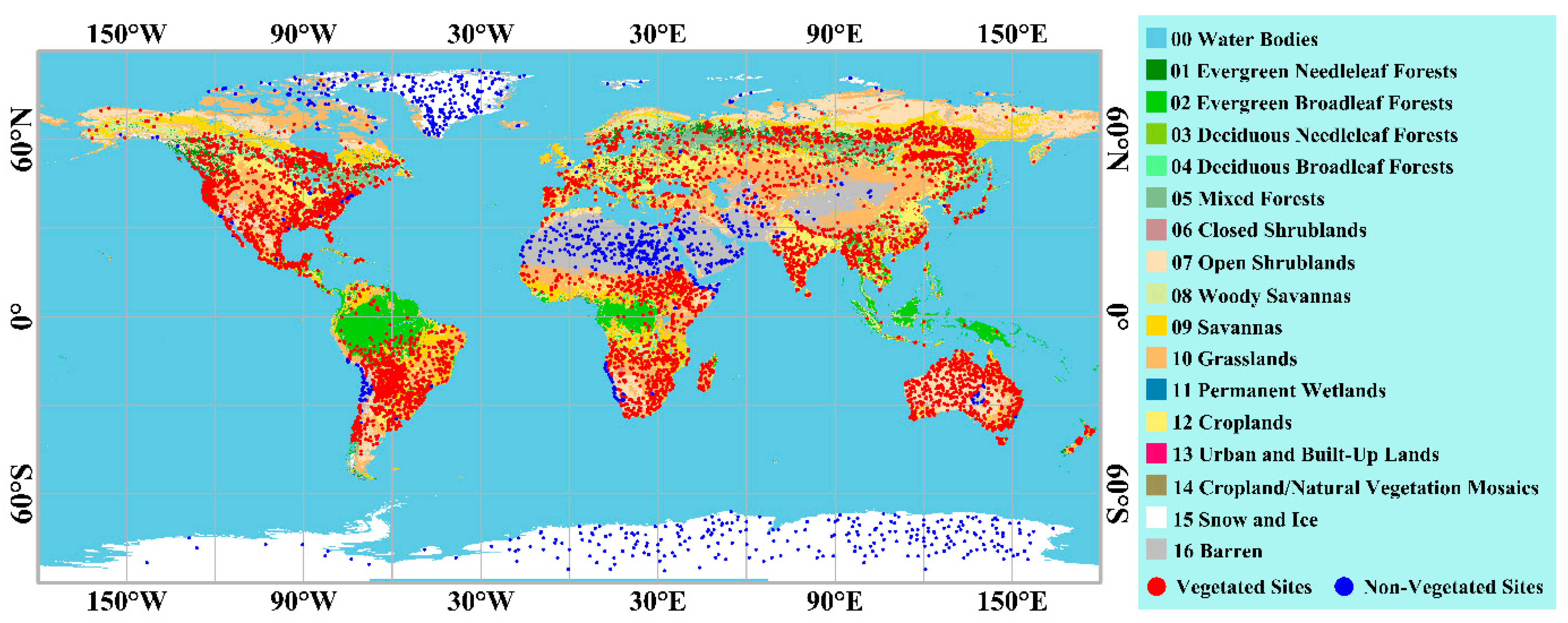
2.1. POLDER BRDF Database

In this study, we used a high-quality BRDF database published by Breon et al. [26], which is recommended by the authors to be applied in assessing the typical variabilities of natural surface reflectances or evaluating the new BRDF models (https://doi.pangaea.de/10.1594/PANGAEA.864090 (accessed on 27 January 2022)). This database provides a set of high-quality reflectance observations from the POLDER-3 sensor collected from January 2008 to December 2008. It only includes observations from 2008, as this year was the best in terms of data acquisition continuity. Moreover, these observations are available without significant cloud or aerosol contamination and were acquired with various observation geometries. The targets are classified into 16 classes of IGBP (International Geosphere-Biosphere Programme) land cover types (without water), the selection of which requires spatial representativeness within the class [14]. The POLDER-3 observes the surface target from up to 16 directions (14 on average) per overflight with a maximum View Zenith Angle (VZA) close to 70° [26]. These allow us to easily compare the fitting ability of the RTLSR model over different land cover types and observation geometries.

The BRDF database contains six bands of reflectance data, and only the red and Near-Infrared (NIR) bands (centered at 670 nm and 865 nm, respectively) were used in this study. It also provides a metric called Aero, which is a non-quantitative indication of the aerosol load retrieved from POLDER measurements. Aero = 0 means minimal aerosol load, whereas Aero = 15 represents a high aerosol load. Only observations with Aero ≤ 5 are used in our study. Figure 1 shows the global distribution of POLDER BRDF database sites.

2.2. Linear Kernel-Driven Models and Retrieval Method

In optics, BRDF is defined as the ratio of the radiance in the direction of the exit beam to the irradiance caused by the entrance beam [1]. However, it cannot be strictly measurable under natural conditions. It essentially describes the anisotropy of the irradiated object. In remote sensing, since pixels are usually non-uniform surfaces with a certain area, the BRDF cannot be defined effectively, while the definition of parameters, such as reflectance, still holds. Therefore, the measured reflectance data are often referred to as BRDF [31,32]. BRDF is usually used to represent the bidirectional reflectance distribution to quantitatively describe the anisotropy of the land surface [22,33]. The linear kernel-driven model, originally proposed by Roujean et al. [8], is usually used to retrieve bidirectional reflectance. It can be formalized as the empirically weighted sum of several scattering components [34]. The equation can be expressed as:

$$R({\theta }_s,{\theta }_v,\phi ,\lambda )=f_{iso}(\lambda )+f_{vol}(\lambda )K_{vol}({\theta }_s,{\theta }_v,\phi )+f_{geo}(\lambda )K_{geo}({\theta }_s,{\theta }_v,\phi )$$

(1)

where $R({\theta }_s,{\theta }_v,\phi ,\lambda )$ is the reflectance in waveband $\lambda$, which is a function of the Solar Zenith Angle (SZA) ${\theta }_s$, VZA ${\theta }_v$, and Relative Azimuth Angle (RAA) $\phi$. $f_{iso}(\lambda )$, $f_{vol}(\lambda )$, and $f_{geo}(\lambda )$ are the weight components of the isotropic scattering kernel (considered as 1), volume-scattering kernel $K_{vol}({\theta }_s,{\theta }_v,\phi )$, and geometric-optical kernel $K_{geo}({\theta }_s,{\theta }_v,\phi )$.

Given reflectance observations $\rho ({\theta }_s,{\theta }_v,\phi ,\lambda )$, the minimization $\frac{\partial e^2}{\partial f_k}=0$ of a least-squares error function:

$$e^2(\lambda )=\frac{1}{d}{\displaystyle \sum _l\frac{{({\rho }_l({\theta }_s,{\theta }_v,\phi ,\lambda )-R_l({\theta }_s,{\theta }_v,\phi ,\lambda ))}^2}{w_l(\lambda )}}$$

(2)

leads to analytical solutions for the weight components $f_k$ of the kernels:

$$f_k(\lambda )={\displaystyle \sum _i\left\{{{\displaystyle \sum _j\frac{{\rho }_j({\theta }_s,{\theta }_v,\phi ,\lambda )K_i({\theta }_s,{\theta }_v,\phi )}{w_j(\lambda )}\times \left({\displaystyle \sum _l\frac{K_i({\theta }_s,{\theta }_v,\phi )K_k({\theta }_s,{\theta }_v,\phi )}{w_l(\lambda )}}\right)}}^{-1}\right\}}$$

(3)

where $w_l(\lambda )$ is the weight given to each observation. In this study, all eligible observations were given the same weight [6]. Additionally, $d$ are the degrees of freedom (number of observations minus number of parameters $f_k$).

Some extended forms of the kernel-driven model typically introduce more input parameters or kernels to improve fitting ability. Therefore, Equation (1) may not be a general form of the kernel-driven models. In this paper, the kernel-driven models can be considered as a general term for models that work in the same way (kernel drive).

2.2.1. RTLSR Model

The RTLSR model is widely used for its excellent fitting ability among many kernel-driven models, which consists of the volume-scattering kernel RossThick and the geometric-optical kernel LiSparseReciprocal. The RossThick kernel was derived by Roujean et al. [8] based on the radiative transfer theory of Ross [35], which is used to calculate the bidirectional reflectance above a horizontally homogeneous plant canopy with large values of the LAI (the formula for the RossThick kernel is given in detail in Appendix A). The LiSparseReciprocal kernel is a reciprocal form of the geometric-optical kernel LiSparse [6,17,36]. The LiSparse kernel is the approximation of a geometric-optical mutual shadowing model by Li and Strahler [37] derived by Wanner et al. [9]. It is modeled as:

$$\begin{array}{ll}{K}_{\mathrm{LiSparse}}& =O({\theta }_s{}^{\prime },{\theta }_v{}^{\prime },\phi )-\sec {\theta }_s{}^{\prime }-\sec {\theta }_v{}^{\prime }+\frac{1}{2}(1+\cos {\xi }^{\prime })\sec {\theta }_v{}^{\prime }\\ & =P({\theta }_s{}^{\prime },{\theta }_v{}^{\prime },\phi )\sec {\theta }_v{}^{\prime }-B({\theta }_s{}^{\prime },{\theta }_v{}^{\prime },\phi )\end{array}$$

(4)

where $B({\theta }_s{}^{\prime },{\theta }_v{}^{\prime },\phi )=\sec {\theta }_s{}^{\prime }+\sec {\theta }_v{}^{\prime }-O({\theta }_s{}^{\prime },{\theta }_v{}^{\prime },\phi )$, $P({\theta }_s{}^{\prime },{\theta }_v{}^{\prime },\phi )=\frac{1}{2}(1+\cos {\xi }^{\prime })$ and

$$O=\frac{1}{\pi }(t-\sin t\cos t)(\sec {\theta }_s{}^{\prime }+\sec {\theta }_v{}^{\prime })$$

(5)

$$\cos t=\frac{h}{b}\frac{\sqrt{D^2+{(\tan {\theta }_s{}^{\prime }\tan {\theta }_v{}^{\prime }\sin \phi )}^2}}{\sec {\theta }_s{}^{\prime }+\sec {\theta }_v{}^{\prime }}$$

(6)

$$D=\sqrt{{\tan }^2{\theta }_s{}^{\prime }+{\tan }^2{\theta }_v{}^{\prime }-2\tan {\theta }_s{}^{\prime }\tan {\theta }_v{}^{\prime }\cos \phi }$$

(7)

$$\cos {\xi }^{\prime }=\cos {\theta }_s{}^{\prime }\cos {\theta }_v{}^{\prime }+\sin {\theta }_s{}^{\prime }\sin {\theta }_v{}^{\prime }\cos \phi$$

(8)

$${\theta }_{s,v}{}^{\prime }={\tan }^{-1}(\frac{b}{r}\tan {\theta }_{s,v})$$

(9)

$$\phi =\mathrm{abs}({\phi }_s-{\phi }_v),0\le \varphi <\pi$$

(10)

where ${\phi }_s$ and ${\phi }_v$ are the solar and view azimuth angles. The LiSparse kernel was designed for sparsely located clumps and associated shadows. The approximation made for LiSparse is $e^{-x}=1-x$, where $x$ is the area proportion of this clump plus shadow, roughly proportional to $\sec {\theta }_v$. Therefore, LiSparse kernel has poor ability for extrapolation at large VZAs, especially when SZA is large, where negative reflectance may appear even the kernel fits the sampled observations very well. To alleviate this problem, the LiSparseReciprocal kernel was proposed based on the reciprocity principle [38]. The kernel is modeled as:

$$K_{\mathrm{LiSparseR}}=P({\theta }_s{}^{\prime },{\theta }_v{}^{\prime },\phi )\sec {\theta }_s{}^{\prime }\sec {\theta }_v{}^{\prime }-B({\theta }_s{}^{\prime },{\theta }_v{}^{\prime },\phi )$$

(11)

In the above equations, the parameters $\frac{b}{r}$ and $\frac{h}{b}$ are used to describe the relative crown shape and relative crown height, respectively. The LiSparseReciprocal kernel set to $\frac{b}{r}=1$ and $\frac{h}{b}=2$ is adopted by the MODIS BRDF/albedo algorithm, which is also used in this study. More details on the derivation of this kernel can be found in [9].

2.2.2. RTLT Model

The Helmholtz principle of reciprocity has been proved that it suffers scale effect over the heterogeneous land surface and thus does not generally apply to the scale of a remote-sensing pixel [39]. To address this issue, Li et al. [17] improved a new kernel with better extrapolation capabilities, LiTransit, which is proposed to replace the LiSparseReciprocal kernel in the next version of AMBRALS. The RTLT model was generated by combining the volume-scattering kernel RossThick and the geometric-optical kernel LiTransit. The LiTransit kernel can be expressed as:

$$K_{\mathrm{LiTransit}}=\{\begin{array}{c}{K}_{\mathrm{LiSparse}},\hspace{0.17em}\hspace{0.17em}B({\theta }_s{}^{\prime },{\theta }_v{}^{\prime },\phi )\le 2\\ \frac{2\cdot K_{\mathrm{LiSparse}}}{B({\theta }_s{}^{\prime },{\theta }_v{}^{\prime },\phi )},\hspace{0.17em}\hspace{0.17em}B({\theta }_s{}^{\prime },{\theta }_v{}^{\prime },\phi )>2\end{array}$$

(12)

In this paper, the RTLT model is tried to process the data with large SZA.

2.2.3. RTLSRS Model

The RTLSRS (RossThick-LiSparseR-Snow) model developed by Jiao et al. [21] was designed to characterize the scattering properties of the snow surface better. The snow kernel in the model can be seen as a correction kernel based on the Asymptotic Radiative Transfer (ART) model, which assumes that snow can be modeled as a semi-infinite, plane-parallel, weakly absorbing light scattering layer. The snow kernel adopts a correction term with a free parameter $\alpha$ to correct the analytic form of the ART model. The snow kernel and RTLSRS model can be written as follows:

$$K_{\mathrm{snow}}=R_0({\theta }_{\mathrm{s}},{\theta }_{\mathrm{v}},\phi \left)\right(1-\alpha \cdot \cos \xi \cdot e^{-\cos \xi })+0.04076\alpha -1.1081$$

(13)

$$\begin{array}{ll}R({\theta }_s,{\theta }_v,\phi ,\lambda )& =f_{iso}(\lambda )+f_{vol}(\lambda )K_{vol}({\theta }_s,{\theta }_v,\phi )+f_{geo}(\lambda )K_{geo}({\theta }_s,{\theta }_v,\phi )\\ & +f_{snow}(\lambda )K_{snow}({\theta }_s,{\theta }_v,\phi )\end{array}$$

(14)

where $R_0$ refers to the surface reflectance of a semi-infinite, non-absorbing media layer at zero absorption. In this paper, the $\alpha$ was set to 0.3 as recommended [21]. The RTLSRS model with the additional snow kernel can be seen as an extended form of the kernel-driven models.

2.3. Comparative Analysis

The kernel-driven models can fit the kernel coefficients by taking the reflectance and sun-sensor geometries data from the POLDER BRDF database as the input data [6]. This database contains data at different sites for different months and IGBP (detailed information on how they are organized can be found in [26]). The coefficients of the kernel-driven model were calculated using one-month valid data for each site. We then used these coefficients to retrieve the corresponding reflectance. By comparing the retrieved reflectance with observational reflectance, the applicability of the RTLSR model in different scenarios can be evaluated. The NDVI (Normalized Difference Vegetation Index) was used to characterize the vegetation densities. The fitting ability of the RTLSR model was comprehensively compared under different IGBP and NDVI, sun-sensor geometries, and spatial and temporal conditions. For statistical data analysis, we restricted only 20 or more eligible sites to participate, and eligible sites must have at least 16 observations with a low aerosol load (Areo ≤ 5).

We quantified the model fitting residuals using the Root-Mean-Square-Error (RMSE), and defined an Optimization Ratio (OR) for comparing the performance of other models with the RTLSR model. The corresponding formulas are as follows:

$$\begin{array}{l}RMSE=\sqrt{\frac{1}{n-1}{\displaystyle \sum _{i=1}^n{(y_i-x_i)}^2}}\\ OR=\frac{RMS{E}_{\mathrm{RTLSR}}-RMS{E}_{\mathrm{Other}}}{RMS{E}_{\mathrm{RTLSR}}}\times 100\%\end{array}$$

(15)

where n is the number of reflectances, and x and y are the observed and retrieved reflectances, respectively. $RMS{E}_{\mathrm{RTLSR}}$ and $RMS{E}_{\mathrm{Other}}$ are the RMSE of RTLSR and other models, respectively.

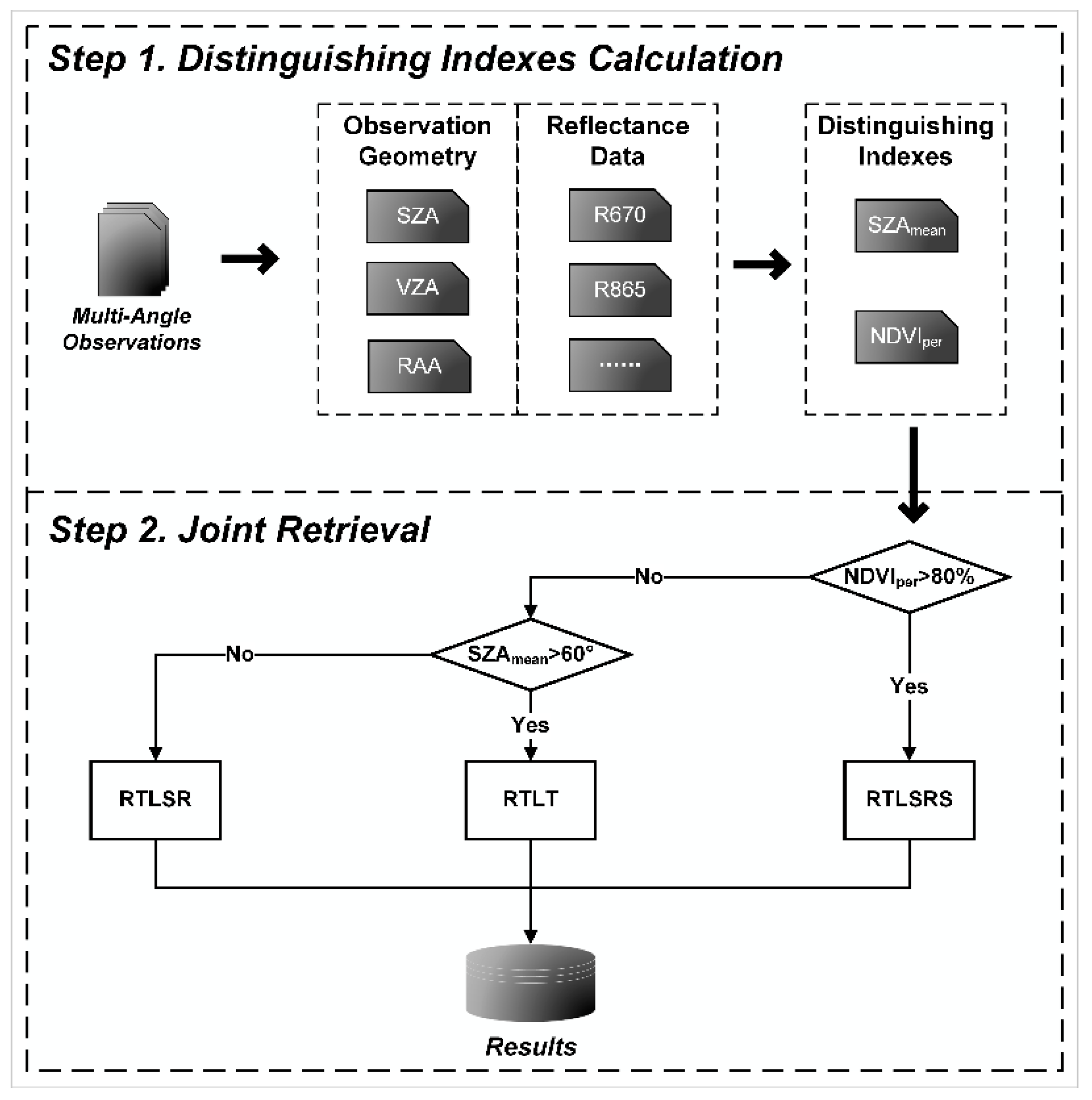
2.4. Simple Joint Retrieval Strategy

In the results of the adaptability comparison of the RTLSR model to different observational conditions (shown in Section 3.1), the model shows a poor fitting ability to non-vegetated surfaces and large SZA conditions. This makes the model exhibit larger fitting residuals at high latitudes. As an exploration, we designed the SJRS and its workflow is shown in Figure 2.

First, we extracted the reflectance and observation geometry information in red and NIR bands from the quality-controlled POLDER sites. Then, the mean SZA (SZA_mean) and the percentage of NDVI less than 0 at each site (NDVI_per) were calculated. We used NDVI_per to determine whether the site is widely covered by snow or ice. If NDVI_per is greater than 80%, the SJRS would use the RTLSRS model to process it. Otherwise, we would further determine whether SZA_mean is greater than 60°, if yes, the site would be retrieved using RTLT. If SZA_mean is less than 60°, the RTLSR model would be used. Finally, the results of each model are integrated into the retrieval results for the global land surface sites. It is worth noting that the thresholds SZA_mean and NDVI_per are adjustable parameters. In this paper, they were set to 60° and 80% empirically for the initial exploration of the joint application of the multiple models.

3. Results

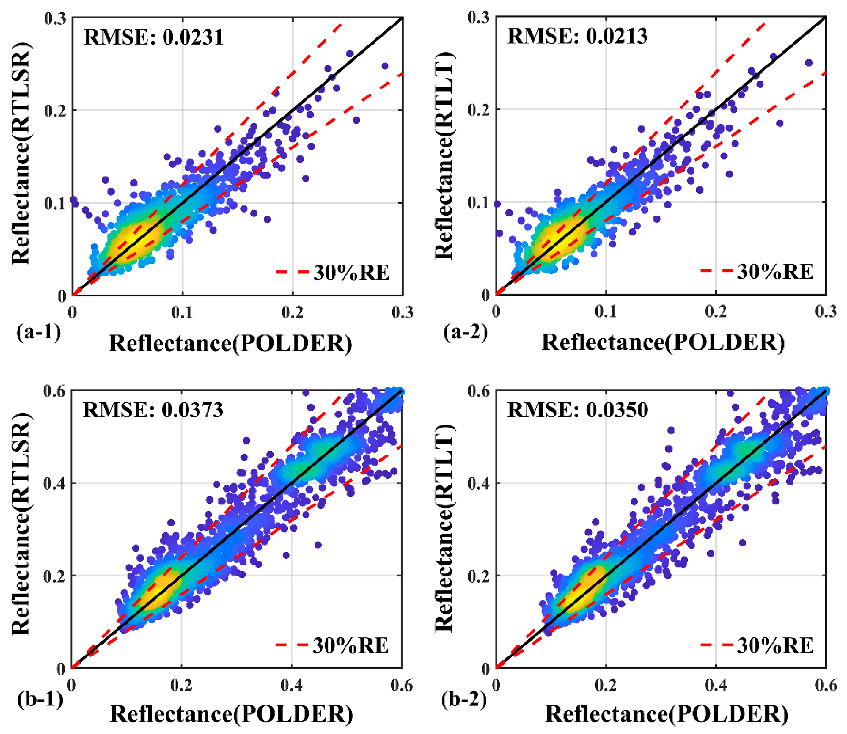
3.1. Applicability Comparison of the RTLSR Model

In this section, the POLDER database was used to revisit the fitting ability of the RTLSR model under different observational conditions. The relevant results are given in Figure 3, Figure 4 and Figure 5. The performance of the RTLSR model over different land covers is given in Figure 3. Overall, the mean fitting residuals of the RTLSR model for all scenarios are 0.0139 and 0.0159 in the red and NIR bands, respectively, indicating a good fitting ability of RTLSR. However, it can be noted that the RTLSR model shows larger fitting residuals in both the red (Figure 3(a-1)) and NIR (Figure 3(a-2)) bands over snow and ice, urban and built-up lands, and evergreen needleleaf forests. Especially for urban and built-up lands, the RMSE is up to 0.1298 (red) 0.0995 (NIR). This is due to the fact that the RTLSR model does not fit well to land covers with large forward scattering. The fitting residuals of the RTLSR model are relatively small over other land covers. For all NDVI levels, the fitting residuals are small over open shrublands and woody savannas. At the same time, the fitting residuals decreased as NDVI increased, as in urban and built-up lands, deciduous broadleaf forests, and mixed forests in the red band. For a more intuitive representation, the fitting residuals of the RTLSR model in vegetated and non-vegetated lands, classified into three levels of vegetation density based on the NDVI values, can be seen in Figure 3(b-1,b-2). The RTLSR model shows lower fitting residuals over vegetated lands, and the fitting residuals decrease with increasing vegetation density. Over non-vegetated lands, the RMSE reaches 0.0424 when NDVI < 0.3 and decreases to 0.0090 when the NDVI > 0.3 in the red band. In the three NDVI levels of vegetated lands, the RMSE is 0.0126, 0.0085, and 0.0042, respectively. The phenomenon also exists for the NIR band: the RMSE is 0.0351 on the non-vegetated lands when NDVI < 0.3 and decreases to 0.0093 when NDVI > 0.3. For the three NDVI levels of vegetated lands, the RMSE is 0.0137, 0.0111, and 0.0102, respectively. In summary, the RTLSR model shows stronger adaptability to densely vegetated lands.

We also explored the influence of sun-sensor geometries on the fitting ability of the RTLSR model, as they are the input parameters of the kernel functions. The relationship between the sun-sensor geometries and the fitting residuals of the RTLSR model in the red (Figure 4a) and NIR (Figure 4b) bands were analyzed. In Figure 4(a-1,b-1), for a given RAA, the color of the dots changes from dark blue to red as the SZA increases from 0° to 75°, which means the values of the RMSE increase with SZA. Figure 4(a-2,b-2) show the change in fitting residuals when the VZA of the retrieved observations are different for a given RAA. The relationship between the fitting residuals and VZA is not clear. From the above statistics, it can be seen that the variations of the SZA greatly affect the fitting ability of the RTLSR model, and the fitting residuals of the RTLSR model increase when SZA becomes larger. Therefore, when SZA is large, the applicability of the RTLSR model needs to be further considered.

Climate, land cover, vegetation density, and sun-sensor geometry are affected by latitude and time, which means that the RTLSR model should have different applicability at different latitudes and times. In the present study, we analyzed the spatial and temporal characteristics of the fitting residuals of the RTLSR model using observations at different latitudes and times (Figure 5). It can be found that the larger fitting residuals are at the four corners in the heat maps of the red and NIR bands. As the top line plot show, the mean fitting residuals of RTLSR reach 0.0444 and 0.0483 at high latitudes in the red and NIR bands, respectively. The reason should be that at high latitudes the land cover is mainly non-vegetated lands (wasteland or snow and ice) and vegetation is sparse, the SZA is also larger. The mean fitting residuals on different months are reflected in the right line plot in the red band (Figure 5a). The relationship between RMSE and time is weak. This suggests that the adaptability of the RTLSR model is not strongly correlated with time. Similar laws are presented in the NIR band (Figure 5b). The results reflected in Figure 5 are consistent with the previous analysis.

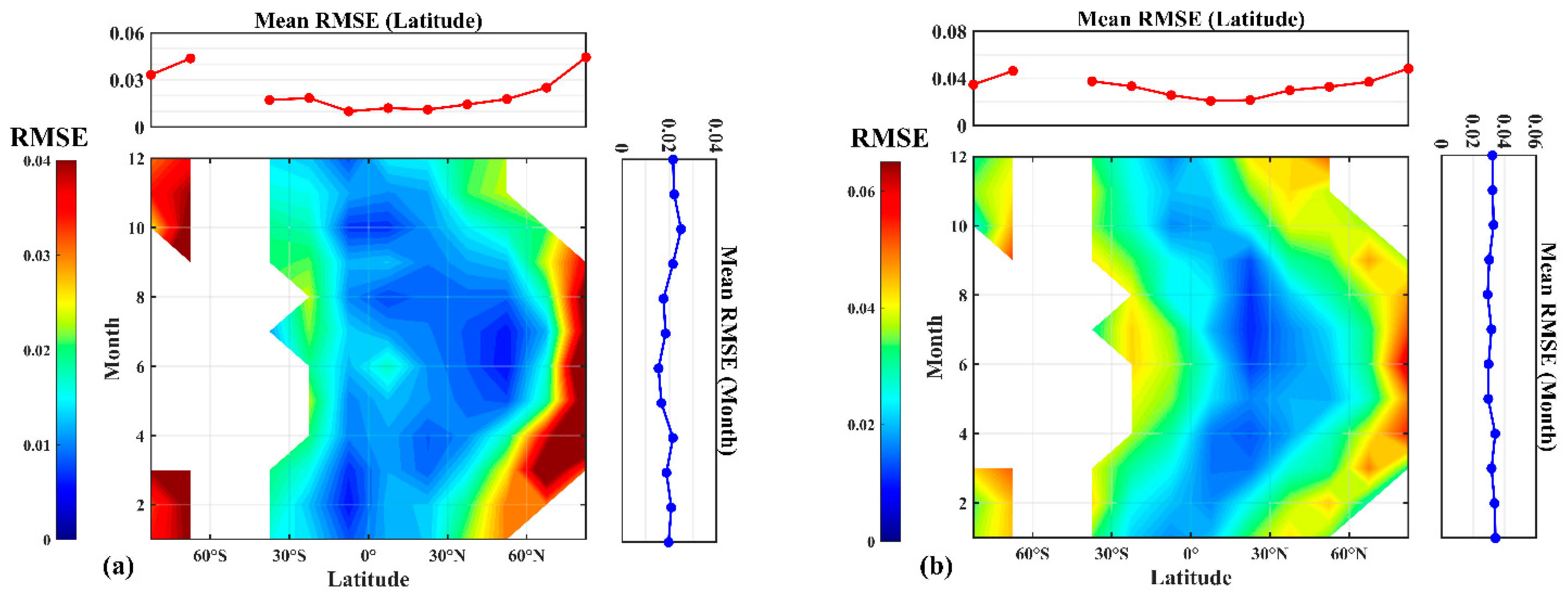
3.2. Joint Application of Kernel-Driven Models

The RTLSR model performs well under most of the observational conditions. It still exhibits large errors at high latitudes due to changes in the land cover and observation geometry. In this section, whether the SJRS can compensate for the shortcomings of a single model is explored. The relevant results are presented in Figure 6, Figure 7 and Figure 8. In Figure 6, the RTLSR and RTLT models are compared using quality-controlled observations with large SZA (SZA > 60°). In the red band (Figure 6a), with the 30% RE (Relative Error) lines as the reference, the predicted results of the RTLT model are more concentrated around the 1:1 line compared to those of the RTLSR model. This means that the predicted reflectance of the RTLSR model deviates more from the POLDER observed reflectance. The results statistics show that the mean RMSE of the RTLSR model in the red band is 0.0231, while the mean RMSE of the RTLT model is 0.0213. This finding is similar in the NIR band (Figure 6b): the mean RMSE of the RTLSR model is 0.0373, while the mean RMSE of the RTLT model is 0.0350. These suggest that the RTLT model does have more reliable extrapolation capability compared to the RTLSR model, and can retrieve these observed data with large SZA conditions more accurately.

The optimized performance of the RTLSRS model compared to the RTLSR model over the snow and ice lands (IGBP = 15) is shown in Figure 7. The horizontal and vertical axes of the figure indicate the RMSE exhibited by the RTLSR and RTLSRS models, respectively. This means that the fitting residual of the RTLSRS model is smaller than that of the RTLSR model in the site when the point is to the lower right of the 1:1 line. Similarly, if the point is on the upper left of the 1:1 line, it means that the fitting residual of the RTLSRS model is larger. Additionally, the darker orange color represents the larger OR of the RTLSRS model, while the darker blue color represents the larger negative OR. In the red (Figure 7a) and NIR (Figure 7b) bands, we can observe that most of the points appear in the lower right of the 1:1 line, which means that the RTLSRS model outperforms the RTLSR model at most of the sites. Among all sites, the max OR of 93.6% and 93.8% for the RTLSRS model were achieved in the red and NIR bands, respectively. The mean RMSE of the RTLSR model can reach 0.0413 and 0.0450 in the red and NIR bands, while the mean RMSE of the RTLSRS model are only 0.0248 and 0.0261. These results suggest that the RTLSRS model can better characterize the bidirectional reflectance of the snow and ice surface, which should effectively reduce the fitting residuals of the snow and ice covered sites.

We compared the differences between using a single RTLSR model and the SJRS using the three kernel-driven models in Figure 8, which uses the same form as Figure 5 to show the fitting residuals for using the hybrid retrieval strategy at different latitudes and months. As can be seen in Figure 8, the fitting residuals of the SJRS are significantly reduced at high latitudes compared to using a single RTLSR model, in comparison to Figure 5. In the Antarctic region, for example, the mean RMSE of the RTLSR model reaches 0.0333 (90° S < latitude < 75° S) and 0.0438 (75° S < latitude < 60° S) in the red band, while the mean RMSE of SJRS is only 0.0194 and 0.0226, respectively. In the NIR band, the mean RMSE of the RTLSR model can reach 0.0347 (90° S < latitude < 75° S) and 0.0463 (75° S < latitude < 60° S), while the mean RMSE of SJRS is only 0.0196 and 0.0225. Similarly, in the Arctic region, the SJRS is also effective in reducing the fitting residuals. Comparing the mean RMSE from different months, the mean RMSE of SJRS are smaller than those of the RTLSR model. These suggest that the SJRS using the three kernel-driven models can effectively compensate for the shortcomings of the retrieval method using a single RTLSR model.

4. Discussion

4.1. Applicability Differences of the RTLSR Strategy

In the results section, the RTLSR model shows a large applicability gap under different observation conditions. There are two important factors: (1) the type of land cover and vegetation cover density, and (2) the SZAs of reflectance used for the retrieval. These two factors cause the RTLSR model to exhibit larger fitting residuals at high latitudes (RMSE can reach up to 0.1 in some pixels, which is also a large fitting residual even for the snow surface). In this section, we discuss why the RTLSR model is significantly influenced by these two factors. Additionally, the impact of the applicability differences on the application of the RTLSR model is illustrated.

The kernel-driven model is a semi-empirical model with the kernels that provide physical condition constraints for an empirical fit. The approximate physical basis on which the kernels rest constrains, in a meaningful way, the possible BRDF shapes in unobserved regions of the viewing and illumination hemisphere. Therefore, the RossThick and LiSparseR kernels of the RTLSR model are the keys to its applicability in different conditions. The RossThick kernel was derived based on the radiative transfer theory of Ross [8], which is used to calculate the bidirectional reflectance above a horizontally homogeneous plant canopy [35]. Additionally, the LiSparseR kernel is the approximation of a geometric-optical model, which is used to describe the bidirectional properties of discrete canopies [9]. This means that the two kernels are both more suitable for vegetated lands and cannot capture large forward scattering, which is why the RTLSR model exhibits large fitting residuals on snow surfaces and urban and built-up lands. Additionally, it is clear why the fitting residuals of the RTLSR model are negatively correlated with vegetation cover density. The RTLSR model performs poorly over evergreen needleleaf forests due to the clumped (nonrandom) arrangement of the needle area in the crown [40], which is inconsistent with the assumptions in the RossThick kernel. For the second factor (the SZAs of reflectance used for retrieval), this may be due to the longer path of photons through the canopy caused by large SZA [41], and the extinction process becomes more complicated, resulting in more difficult modeling of the bidirectional reflectance [17]. Under the influence of the superposition of the two factors, the RTLSR model shows poorer applicability at high latitudes.

Currently, in most BRDF/Albedo global product productions and related large-scale researches, a single kernel-driven model was used. They did not take into account the difference in applicability of a single model under different conditions. This would lead to different absolute accuracies in different regions in the global product. Meanwhile, this may also lead to erroneous conclusions in large-scale researches. Taking the RTLSR model used in the experiments of this paper as an example, it exhibits a large difference in absolute accuracy on vegetated lands and snow surfaces. When it is applied to high altitude mountains, there may be a problem of a large gap of retrieval accuracy. This is cannot be neglected in studies. Therefore, for this type of study, different models should be used in a targeted manner to ensure the best performance.

Many scholars developed many new kernels and kernel-driven models to improve the applicability of the models, which are summarized in Appendix A. These studies provide a rationale for the joint application of multiple models. In this paper, we tried to use the SJRS for a large-scale retrieval. The results show that this approach is effective in reducing the applicability differences. Therefore, we believe that this direction has great potential for exploration, which may be a better choice for global product production and large-scale researches.

4.2. Future Development and Application of the Kernel-Driven Models

Compared to the physical model, the semi-empirical kernel-driven models do not need to describe the details of the physical processes of light scattering in the scene and do not require too much prior knowledge of the scene parameters. At the same time, the linearly weighted form of the kernel-driven models allows for fast retrieval, making it easier to apply to large-scale experimental data processing than other models. This is the main reason why the kernel-driven models have been adopted by many sensors [9].

However, the existing kernels of the kernel-driven models are all based on a physical approximation of a particular hypothetical scenario. This means that the kernels have similar characteristics to the physical model: no kernel is equally suitable for every scenario. They have different adaptability for different scenarios. When the application scenario is closer to the assumed, the kernel-driven model is able to retrieve the results more accurately. On the contrary, if the application scenario deviates significantly from the kernel assumptions, the kernel-driven model exhibits poor adaptability. As demonstrated in the results section, the RTLSR model based on the vegetation cover scenario assumptions exhibit large fit residuals in the non-vegetation cover scenario. On the contrary, the RTLSRS model designed to describe the large forward scattering of the snow surface shows better fitting results at the sites with IGBP = 15 (snow and ice).

As mentioned in Appendix A for the numerous kernels and improved kernel-driven models, they are designed to be better adapted to a certain scenario. However, most of the existing BRDF/albedo products are produced by a single kernel-driven model, which inevitably leads to different degrees of fitting residuals under different observational conditions. Many studies that adopted kernel-driven models have also directly used the so-called widely used kernel-driven model without screening comparisons, which may also have the problem of adaptation differences. Therefore, there are several issues worth noting in future research work on kernel-driven models: (1) more comprehensive comparisons and evaluations of existing models are necessary to inform the selection of models for application; (2) in global product productions and large-scale studies, we should try to combine different models for different application scenarios, which can compensate for the shortcomings of the results due to the difference in adaptability; and (3) future work on the improvement of the kernel-driven models or their kernels may allow for more refined assumptions and modeling, which could improve the accuracy of retrieval. Although this would require more input parameters and prior knowledge, the development of existing computational power should be fully satisfying.

4.3. Limitations of the Study and Future Work

There are still some limitations in this study. First, the applicability comparison for the RTLSR model may be influenced by the coarser resolution of the POLDER-3 sensor (6 km × 7 km). Therefore, the conclusions obtained may be unacceptable at other scales. Second, in this study, we focused only on the red and NIR bands. The ground substance has different spectral properties for different wavelengths. Therefore, the proposed joint-use strategy based on the results in the red and NIR bands may not be applicable for other bands. Third, while SJRS performs better at high latitudes, it is only a simple combination of three kernel-driven models, so more rigorous validations and optimizations are necessary for practical application in the future.

To address the limitations of this paper and some of the problems facing the field, our future work will focus on the following: (1) we will conduct a more comprehensive comparison and evaluation of the existing models and summarize a set of model selection references, and (2) use targeted modeling to address the shortcomings of existing models and attempt to propose a set of joint retrieval strategies applicable to various global observational conditions.

5. Conclusions

This study comprehensively compared the applicability of the kernel-driven model represented by the RTLSR kernels to revisit its performance under different observational conditions using the filtered high-quality POLDER BRDF database. Further, we explored the potential for the joint application of multiple kernel-driven models. The results show that the RTLSR model performs well which has small RMSE under most observational conditions. However, over different land covers, the RTLSR model has a better fitting ability over densely vegetated surfaces, while it shows more than twice as many fitting residuals on non-vegetated lands compared to vegetated. Under different sun-sensor geometries, the fitting residuals are positively correlated with SZA. The RTLSR model shows poorer fitting ability when SZA is large. Therefore, the RTLSR model shows better fitting ability at mid and low latitudes due to the better observational conditions. In contrast, the RTLSR model exhibits larger fitting residuals at high latitudes due to the increased proportion of non-vegetation covered lands and large SZA observational conditions. As an exploration, we proposed a model combination strategy, SJRS, by combining different models using the distinguishing indexes. The SJRS shows better performance at high latitudes. Based on this, we analyzed in depth the root causes for the differences in applicability of RTLSR models and the development potential of the joint application of multiple kernel-driven models. Additionally, we discussed the future direction of the kernel-driven models. These conclusions contribute to a better understanding of the fitting ability of the RTLSR model and are helping to improve the use of kernel-driven models. The proposed view of joint application of models also has the potential to improve the ability to describe the anisotropy of land surface reflectance.

References

1. Nicodemus, F.E.; Richmond, J.C.; Hsia, J.J.; Ginsberg, I.W.; Limperis, T. Geometrical Considerations and Nomenclature for Reflectance. In Final Report National Bureau of Standards; US Department of Commerce, National Bureau of Standards: Washington, DC, USA, 1977; Volume 160. [Google Scholar]
2. Schaepman-Strub, G.; Schaepman, M.E.; Painter, T.H.; Dangel, S.; Martonchik, J.V. Reflectance quantities in optical remote sensing—definitions and case studies. Remote Sens. Environ. 2006, 103, 27–42. [Google Scholar] [CrossRef]
3. Tanioka, Y.; Cai, Y.; Ida, H.; Hirota, M. A spatial relationship between canopy and understory leaf area index in an old-growth cool-temperate deciduous forest. Forests 2020, 11, 1037. [Google Scholar] [CrossRef]
4. Xu, B.; Park, T.; Yan, K.; Chen, C.; Zeng, Y.; Song, W.; Yin, G.; Li, J.; Liu, Q.; Knyazikhin, Y. Analysis of global LAI/FPAR products from VIIRS and MODIS sensors for spatio-temporal consistency and uncertainty from 2012–2016. Forests 2018, 9, 73. [Google Scholar] [CrossRef] [Green Version]
5. Pokrovsky, O.; Roujean, J.-L. Land surface albedo retrieval via kernel-based BRDF modeling: I. Statistical inversion method and model comparison. Remote Sens. Environ. 2003, 84, 100–119. [Google Scholar] [CrossRef]
6. Lucht, W.; Schaaf, C.B.; Strahler, A.H. An algorithm for the retrieval of albedo from space using semiempirical BRDF models. IEEE Trans. Geosci. Remote Sens. 2000, 38, 977–998. [Google Scholar] [CrossRef] [Green Version]
7. Dickinson, R.E. Land processes in climate models. Remote Sens. Environ. 1995, 51, 27–38. [Google Scholar] [CrossRef]
8. Roujean, J.L.; Leroy, M.; Deschamps, P.Y. A bidirectional reflectance model of the Earth’s surface for the correction of remote sensing data. J. Geophys. Res. Atmos. 1992, 97, 20455–20468. [Google Scholar] [CrossRef]
9. Wanner, W.; Li, X.; Strahler, A. On the derivation of kernels for kernel-driven models of bidirectional reflectance. J. Geophys. Res. Atmos. 1995, 100, 21077–21089. [Google Scholar] [CrossRef]
10. Wanner, W.; Strahler, A.; Hu, B.; Lewis, P.; Muller, J.P.; Li, X.; Schaaf, C.B.; Barnsley, M. Global retrieval of bidirectional reflectance and albedo over land from EOS MODIS and MISR data: Theory and algorithm. J. Geophys. Res. Atmos. 1997, 102, 17143–17161. [Google Scholar] [CrossRef] [Green Version]
11. Schaaf, C.B.; Gao, F.; Strahler, A.H.; Lucht, W.; Li, X.; Tsang, T.; Strugnell, N.C.; Zhang, X.; Jin, Y.; Muller, J.-P. First operational BRDF, albedo nadir reflectance products from MODIS. Remote Sens. Environ. 2002, 83, 135–148. [Google Scholar] [CrossRef] [Green Version]
12. Schaaf, C.; Liu, J.; Gao, F.; Strahler, A.H. MODIS albedo and reflectance anisotropy products from Aqua and Terra. Land Remote Sens. Glob. Environ. Change NASA’s Earth Obs. Syst. Sci. ASTER MODIS 2011, 11, 549–561. [Google Scholar]
13. Wang, Z.; Schaaf, C.B.; Sun, Q.; Shuai, Y.; Román, M.O. Capturing rapid land surface dynamics with Collection V006 MODIS BRDF/NBAR/Albedo (MCD43) products. Remote Sens. Environ. 2018, 207, 50–64. [Google Scholar] [CrossRef]
14. Deschamps, P.-Y.; Bréon, F.-M.; Leroy, M.; Podaire, A.; Bricaud, A.; Buriez, J.-C.; Seze, G. The POLDER mission: Instrument characteristics and scientific objectives. IEEE Trans. Geosci. Remote Sens. 1994, 32, 598–615. [Google Scholar] [CrossRef]
15. Bicheron, P.; Leroy, M. Bidirectional reflectance distribution function signatures of major biomes observed from space. J. Geophys. Res. Atmos. 2000, 105, 26669–26681. [Google Scholar] [CrossRef]
16. Bacour, C.; Bréon, F.-M. Variability of biome reflectance directional signatures as seen by POLDER. Remote Sens. Environ. 2005, 98, 80–95. [Google Scholar] [CrossRef]
17. Li, X.; Gao, F.; Chen, L.; Strahler, A.H. Derivation and validation of a new kernel for kernel-driven BRDF models. In Remote Sensing for Earth Science, Ocean, and Sea Ice Applications; International Society for Optics and Photonics: Bellingham, DC, USA, 1999; pp. 368–379. [Google Scholar]
18. Gao, F.; Li, X.; Strahler, A.; Schaaf, C. Evaluation of the Li transit kernel for BRDF modeling. Remote Sens. Rev. 2000, 19, 205–224. [Google Scholar] [CrossRef]
19. Maignan, F.; Bréon, F.-M.; Lacaze, R. Bidirectional reflectance of Earth targets: Evaluation of analytical models using a large set of spaceborne measurements with emphasis on the Hot Spot. Remote Sens. Environ. 2004, 90, 210–220. [Google Scholar] [CrossRef]
20. Jiao, Z.; Dong, Y.; Li, X. An approach to improve hot spot effect for the MODIS BRDF/Albedo algorithm. In Proceedings of the 2013 IEEE International Geoscience and Remote Sensing Symposium-IGARSS, Melbourne, Australia, 21–26 July 2013; pp. 3037–3039. [Google Scholar]
21. Jiao, Z.; Ding, A.; Kokhanovsky, A.; Schaaf, C.; Bréon, F.-M.; Dong, Y.; Wang, Z.; Liu, Y.; Zhang, X.; Yin, S.; et al. Development of a snow kernel to better model the anisotropic reflectance of pure snow in a kernel-driven BRDF model framework. Remote Sens. Environ. 2019, 221, 198–209. [Google Scholar] [CrossRef]
22. Yan, K.; Li, H.; Song, W.; Tong, Y.; Hao, D.; Zeng, Y.; Mu, X.; Yan, G.; Fang, Y.; Myneni, R.B. Extending a Linear Kernel-Driven BRDF Model to Realistically Simulate Reflectance Anisotropy Over Rugged Terrain. IEEE Trans. Geosci. Remote Sens. 2021, 60, 1–16. [Google Scholar] [CrossRef]
23. Hu, B.; Wanner, W.; Li, X.; Strahler, A.H. Validation of kernel-driven semiempirical BRDF models for application to MODIS/MISR data. In Proceedings of the IGARSS’96, 1996 International Geoscience and Remote Sensing Symposium, Lincoln, NE, USA, 27–31 May 1996; pp. 1669–1671. [Google Scholar]
24. Hu, B.; Lucht, W.; Li, X.; Strahler, A.H. Validation of kernel-driven semiempirical models for the surface bidirectional reflectance distribution function of land surfaces. Remote Sens. Environ. 1997, 62, 201–214. [Google Scholar] [CrossRef]
25. Huang, X.; Jiao, Z.; Dong, Y.; Zhang, H.; Li, X. Analysis of BRDF and Albedo Retrieved by Kernel-Driven Models Using Field Measurements. IEEE J. Sel. Top. Appl. Earth Obs. Remote Sens. 2013, 6, 149–161. [Google Scholar] [CrossRef]
26. Breon, F.-M.; Maignan, F. A BRDF–BPDF database for the analysis of Earth target reflectances. Earth Syst. Sci. Data 2017, 9, 31–45. [Google Scholar] [CrossRef] [Green Version]
27. Liu, S.; Yan, L.; Yang, B. Degree of Linear Polarization of Land Surfaces: Analyses Using POLDER/PARASOL Measurements. IEEE Access 2020, 8, 200561–200572. [Google Scholar] [CrossRef]
28. Ye, L.; Xiao, P.; Zhang, X.; Feng, X.; Hu, R.; Ma, W.; Li, H.; Song, Y.; Ma, T. Evaluating Snow Bidirectional Reflectance of Models Using Multiangle Remote Sensing Data and Field Measurements. IEEE Geosci. Remote Sens. Lett. 2020, 19, 1–5. [Google Scholar] [CrossRef]
29. Chopping, M.; Moisen, G.G.; Su, L.; Laliberte, A.; Rango, A.; Martonchik, J.V.; Peters, D.P.C. Large area mapping of southwestern forest crown cover, canopy height, and biomass using the NASA Multiangle Imaging Spectro-Radiometer. Remote Sens. Environ. 2008, 112, 2051–2063. [Google Scholar] [CrossRef] [Green Version]
30. Hilker, T.; Coops, N.C.; Hall, F.G.; Black, T.A.; Wulder, M.A.; Nesic, Z.; Krishnan, P. Separating physiologically and directionally induced changes in PRI using BRDF models. Remote Sens. Environ. 2008, 112, 2777–2788. [Google Scholar] [CrossRef] [Green Version]
31. Liang, S.; Li, X.; Wang, J. Quantitative Remote Sensing: Concepts and Algorithms; Science Press: Beijing, China, 2013. [Google Scholar]
32. Wu, S.; Wen, J.; Gastellu-Etchegorry, J.-P.; Liu, Q.; You, D.; Xiao, Q.; Hao, D.; Lin, X.; Yin, T. The definition of remotely sensed reflectance quantities suitable for rugged terrain. Remote Sens. Environ. 2019, 225, 403–415. [Google Scholar] [CrossRef]
33. Hao, D.; Wen, J.; Xiao, Q.; You, D.; Tang, Y. An Improved Topography-Coupled Kernel-Driven Model for Land Surface Anisotropic Reflectance. IEEE Trans. Geosci. Remote Sens. 2020, 58, 2833–2847. [Google Scholar] [CrossRef]
34. Lucht, W.; Roujean, J.L. Considerations in the parametric modeling of BRDF and albedo from multiangular satellite sensor observations. Remote Sens. Rev. 2000, 18, 343–379. [Google Scholar] [CrossRef]
35. Ross, J. The Radiation Regime and Architecture of Plant Stands; Springer Science & Business Media: Berlin/Heidelberg, Germany, 1981. [Google Scholar]
36. Lucht, W. Expected retrieval accuracies of bidirectional reflectance and albedo from EOS-MODIS and MISR angular sampling. J. Geophys. Res. Atmos. 1998, 103, 8763–8778. [Google Scholar] [CrossRef] [Green Version]
37. Li, X.; Strahler, A.H. Geometric-optical bidirectional reflectance modeling of the discrete crown vegetation canopy: Effect of crown shape and mutual shadowing. IEEE Trans. Geosci. Remote Sens. 1992, 30, 276–292. [Google Scholar] [CrossRef]
38. Lucht, W. AMBRALS User’s Guide. Version 3.0; Center for Remote Sensing: Boston, MA, USA, 1998. [Google Scholar]
39. Li, X.; Wang, J.; Strahler, A.H. Apparent reciprocity failure in directional reflectance of structured surfaces. Prog. Nat. Sci. Beijing 1999, 9, 747–752. [Google Scholar]
40. Stenberg, P. Correcting LAI-2000 estimates for the clumping of needles in shoots of conifers. Agric. For. Meteorol. 1996, 79, 1–8. [Google Scholar] [CrossRef]
41. Yin, G.; Li, A.; Zhao, W.; Jin, H.; Bian, J.; Wu, S. Modeling canopy reflectance over sloping terrain based on path length correction. IEEE Trans. Geosci. Remote Sens. 2017, 55, 4597–4609. [Google Scholar] [CrossRef]
42. Jiao, Z.; Schaaf, C.B.; Dong, Y.; Román, M.; Hill, M.J.; Chen, J.M.; Wang, Z.; Zhang, H.; Saenz, E.; Poudyal, R.; et al. A method for improving hotspot directional signatures in BRDF models used for MODIS. Remote Sens. Environ. 2016, 186, 135–151. [Google Scholar] [CrossRef] [Green Version]
43. Bréon, F.M.; Maignan, F.; Leroy, M.; Grant, I. Analysis of hot spot directional signatures measured from space. J. Geophys. Res. Atmos. 2002, 107, AAC 1-1–AAC 1-15. [Google Scholar] [CrossRef]
44. Chen, J.; Cihlar, J. A hotspot function in a simple bidirectional reflectance model for satellite applications. J. Geophys. Res. Atmos. 1997, 102, 25907–25913. [Google Scholar] [CrossRef]
45. Jupp, D.L.; Strahler, A.H. A hotspot model for leaf canopies. Remote Sens. Environ. 1991, 38, 193–210. [Google Scholar] [CrossRef]
46. Wen, J.; Liu, Q.; Xiao, Q.; Liu, Q.; You, D.; Hao, D.; Wu, S.; Lin, X. Characterizing Land Surface Anisotropic Reflectance over Rugged Terrain: A Review of Concepts and Recent Developments. Remote Sens. 2018, 10, 370. [Google Scholar] [CrossRef] [Green Version]
47. Yan, K.; Pu, J.; Park, T.; Xu, B.; Zeng, Y.; Yan, G.; Weiss, M.; Knyazikhin, Y.; Myneni, R.B. Performance stability of the MODIS and VIIRS LAI algorithms inferred from analysis of long time series of products. Remote Sens. Environ. 2021, 260, 112438. [Google Scholar] [CrossRef]
48. Yan, K.; Zhang, Y.; Tong, Y.; Zeng, Y.; Pu, J.; Gao, S.; Li, L.; Mu, X.; Yan, G.; Rautiainen, M. Modeling the radiation regime of a discontinuous canopy based on the stochastic radiative transport theory: Modification, evaluation and validation. Remote Sens. Environ. 2021, 267, 112728. [Google Scholar] [CrossRef]
49. Wu, S.; Wen, J.; Xiao, Q.; Liu, Q.; Hao, D.; Lin, X.; You, D. Derivation of Kernel functions for Kernel-driven reflectance model over sloping terrain. IEEE J. Sel. Top. Appl. Earth Obs. Remote Sens. 2018, 12, 396–409. [Google Scholar] [CrossRef]
50. Cao, B.; Roujean, J.-L.; Gastellu-Etchegorry, J.-P.; Liu, Q.; Du, Y.; Lagouarde, J.-P.; Huang, H.; Li, H.; Bian, Z.; Hu, T. A general framework of kernel-driven modeling in the thermal infrared domain. Remote Sens. Environ. 2021, 252, 112157. [Google Scholar] [CrossRef]
51. Wu, S.; Wen, J.; Liu, Q.; You, D.; Yin, G.; Lin, X. Improving Kernel-Driven BRDF Model for Capturing Vegetation Canopy Reflectance with Large Leaf Inclinations. IEEE J. Sel. Top. Appl. Earth Obs. Remote Sens. 2020, 13, 2639–2655. [Google Scholar] [CrossRef]
52. Dong, Y.; Jiao, Z.; Ding, A.; Zhang, H.; Zhang, X.; Li, Y.; He, D.; Yin, S.; Cui, L. A modified version of the kernel-driven model for correcting the diffuse light of ground multi-angular measurements. Remote Sens. Environ. 2018, 210, 325–344. [Google Scholar] [CrossRef]
Figure 1. Global distribution of the selected POLDER BRDF database sites over the MODIS IGBP land cover map. The red and blue points represent the data in vegetated and non-vegetated lands, respectively.
Forests 13 00435 g001
Figure 2. Workflow of the Simple Joint Retrieval Strategy (SJRS). SZAmean is the mean Solar Zenith Angle (SZA) of the observations at the site. NDVIper is the percentage of the observations with Normalized Difference Vegetation Index (NDVI) < 0 at the site. RAA is Relative Azimuth Angle. R670 and R865 mean the reflectance in red (670 nm) and NIR (865 nm) bands. RTLSR, RTLT, and RTLSRS are the models mentioned in Section 2.2.
Forests 13 00435 g002
Figure 3. Fitting residuals of the RTLSR model for different land covers and NDVI levels in the red (1) and NIR (2) bands; (a-1,a-2) are values of the fitting residuals over different IGBP types, the colors correspond to RMSE values from low (blue) to high (red), and the blank areas mean no data. (b-1,b-2) show the fitting residuals of the RTLSR model on non-vegetated and vegetated lands. IGBP list: 01 Evergreen Needleleaf Forests; 02 Evergreen Broadleaf Forests; 03 Deciduous Needleleaf Forests; 04 Deciduous Broadleaf Forests; 05 Mixed Forests; 06 Closed Shrublands; 07 Open Shrublands; 08 Woody Savannas; 09 Savannas; 10 Grasslands; 11 Permanent Wetlands; 12 Croplands; 13 Urban and Built-Up Lands; 14 Cropland/Natural Vegetation Mosaics; 15 Snow and Ice; and 16 Barren.
Forests 13 00435 g003
Figure 4. Fitting residuals of the RTLSR model in different sun-sensor geometries in the red (a) and NIR (b) bands. (a-1,b-1) are the fitting residuals when SZA is different for a given RAA. (a-2,b-2) are the fitting residuals when VZA is different for a given RAA. In the plots, the radii orient with the RAA and the concentric circles corresponding to the SZA (1) or VZA (2). The missing dots mean no data. The colors correspond to RMSE values from low (blue) to high (red).
Forests 13 00435 g004
Figure 5. Comparison of the fitting residuals of the RTLSR model at different latitudes and months in the red (a) and NIR (b) bands. The colored bars represent RMSE values. The mean RMSE variation in different latitudes and months in the two bands are shown in the line plots above and to the right of the heatmaps, respectively.
Forests 13 00435 g005
Figure 6. Comparison of the reflectance predicted by RTLSR and RTLT with POLDER observations using data with large SZA. The red dotted lines mean 30% RE. The colors correspond to point density from lowest (blue) to highest (yellow). The horizontal axes represent the reflectance from POLDER. The vertical axes represent the reflectance from RTLSR or RTLT model. (a,b) represent the red and NIR bands. (1) and (2) represent the RTLSR and RTLT models, respectively.
Forests 13 00435 g006
Figure 7. Comparison results of the RTLSR and RTLSRS models using data where IGBP is 15 in the POLDER database. Each point represents an observation site. The colors correspond to OR. The horizontal and vertical axes represent the RMSE of the RTLSR and RTLSRS models. The numbers marked in the upper-left corner are the mean RMSE of the RTLSR and the RTLSRS models. (a,b) represent the red and NIR bands, respectively.
Forests 13 00435 g007
Figure 8. Comparison of the fitting residuals of the SJRS at different latitudes and months in the red (a) and NIR (b) bands. The colored bars represent RMSE values. The mean RMSE variation in different latitudes and months in the two bands are shown in the line plots above and to the right of the heatmaps, respectively. The gray lines in the line plots represent the mean RMSE of the RTLSR model, they are the same as the lines in Figure 5.
Forests 13 00435 g008
Publisher’s Note: MDPI stays neutral with regard to jurisdictional claims in published maps and institutional affiliations.