Abstract
A key aspect of vegetation monitoring from LiDAR is concerned with the use of comparable data acquired from multitemporal surveys and from different sensors. Accurate digital elevation models (DEMs) to derive vegetation products, are required to make comparisons among repeated LiDAR data. Here, we aimed to apply an improved empirical method based on DEMs of difference, that adjust the ground elevation of a low-density LiDAR dataset to that of a high-density LiDAR one for ensuring credible vegetation changes. The study areas are a collection of six sites over the Sierra de Gredos in Central Spain. The methodology consisted of producing “the best DEM of difference” between low- and high-density LiDAR data (using the classification filter, the interpolation method and the spatial resolution with the lowest vertical error) to generate a local “pseudo-geoid” (i.e., continuous surfaces of elevation differences) that was used to correct raw low-density LiDAR ground points. The vertical error of DEMs was estimated by the 50th percentile (P50), the normalized median absolute deviation (NMAD) and the root mean square error (RMSE) of elevation differences. In addition, we analyzed the effects of site-properties (elevation, slope, vegetation height and distance to the nearest geoid point) on DEMs accuracy. Finally, we assessed if vegetation height changes were related to the ground elevation differences between low- and high-density LiDAR datasets. Before correction and aggregating by sites, the vertical error of DEMs ranged from 0.02 to −2.09 m (P50), from 0.39 to 0.85 m (NMDA) and from 0.54 to 2.5 m (RMSE). The segmented-based filter algorithm (CSF) showed the highest error, but there were not significant differences among interpolation methods or spatial resolutions. After correction and aggregating by sites, the vertical error of DEMs dropped significantly: from −0.004 to −0.016 m (P50), from 0.10 to 0.06 m (NMDA) and from 0.28 to 0.46 m (RMSE); and the CSF filter algorithm continued showing the greatest vertical error. The terrain slope and the distance to the nearest geoid point were the most important variables for explaining vertical accuracy. After corrections, changes in vegetation height were decoupled from vertical errors of DEMs. This work showed that using continuous surfaces with the lowest elevation differences (i.e., the best DEM of difference) the raw elevation of low-density LiDAR was better adjusted to that of a benchmark for being adapted to site-specific conditions. This method improved the vertical accuracy of low-density LiDAR elevation data, minimizing the random nature of vertical errors and decoupling vegetation changes from those errors.
1. Introduction
A detailed understanding of the magnitude and source of error in LiDAR elevation data and its derived products (i.e., digital elevation models (DEMs) and canopy height models [CHMs]) is necessary for operational use of LiDAR in deriving accurate forest inventory metrics [1,2,3,4]. Errors in the DEMs propagate to vegetation metrics hindering multitemporal comparison [2,3,5]. However, the accuracy of the LiDAR derived DEMs has been often overlooked, although each stage of the modelling process potentially introduces error into the DEMs [6,7].
The general principle of assessing the vertical accuracy of an elevation dataset is to compare those elevations with a reference data, so that statistical parameters, such as the root mean square error (RMSE), can be calculated [8]. Usually, the quantitative assessment of LiDAR elevation data is conducted by comparing “true” terrain checkpoints with LiDAR ground elevations by using DEMs [2,3]. The two DEMs are paired, and an elevation difference is calculated for each pairing (i.e., DEMs of difference) [4,8,9]. The main drawback of this approach is that field surveying is very time consuming and, in some situations, such as in densely forested areas, it is impossible to collect elevation data [10]. When true ground points are not available, interpolated checkpoints from high-density LiDAR ground data have been used as benchmark DEM to either assess the quality, correct other less accurate DEMs, or both, as photogrammetric [9,11] or satellite derived ones (i.e., SRTM) [12,13] using DEMs of difference as procedure. This method has demonstrated being robust to estimate vertical errors but only a few times, it has been used to correct raw elevation values [12,13]. In the latter cases, elevation differences were corrected by means of regression analysis, using several checkpoints but the corrected DEMs continued being affected by the random nature of the elevation errors. Using DEMs of difference as a local pseudo-geoid (i.e., all interpolated points with elevation deviations) allow adjusting less accurate elevation data (e.g., low-density LiDAR) by means of continuous elevation surfaces instead of only checkpoints. This procedure reduces random and other methodological elevation errors increasing the comparability between DEMs and derived vegetation products.
However, distinguishing between real changes and instrumental or methodological noise requires appropriate error analysis to ensure that DEMs of differences are reliable [14]. Moreover, it has been seen that LiDAR errors are not constant within a site line but possibly even neither within a single scan line [15]. The quality of LiDAR elevation data depends on several factors that can be grouped as follows: instrumental, methodological, and site-specific [3,4,5,15,16,17,18]. Developing suitable corrections for such bias has been challenging because several factors contribute to the underestimation or overestimation of elevation with respect to the benchmark one.
The elimination or reduction of instrumental errors in the system parameters have been the focus of LiDAR research [15,19,20,21]. Instrumental errors are related to vertical accuracy, density and spatial distribution of elevation points [8]. Errors in the vertical accuracy of survey instruments (e.g., global navigation satellite systems (GNSS), total stations (TS), the inertial navigation system (INS) and its derived inertial measurement units (IMU)) with respect to a specified vertical datum are one of the most important factors affecting the accuracy of LiDAR derived DEMs [4,22,23]. The misalignment between the IMU system and the scanner (the boresight misalignment) is the largest source of systematic error in a LiDAR and must be addressed before the sensor can be effectively used because errors propagate into the subsequently derived products [20]. These misalignments may cause systematic errors in DEMs of centimetric range over flat terrain, rising to decimetric range over steep slopes [9]. Overall, vertical errors associated with instrumental issues occurred near strip boundaries [15,24] and increasing flying height and off nadir scan angle [9,19]. In addition, LiDAR point densities and spatial distribution of ground LiDAR points have significant effects on the accuracy of derived DEMs [3,10,14,25,26,27]. The quality of the terrain model is determined by the number and distribution of pulses that successfully reach the ground. Dense vegetation obstructs the LiDAR pulses and then, fewer pulses reaching the ground are available for DEM construction [3]. It has been shown that very low pulse density during initial acquisition of LiDAR data is likely to compromise the quality of DEMs and derived canopy metrics [14,28]. However, with high-density LiDAR data point density reduction can be carried out without compromising elevation accuracy [10,27,29].
Moreover, DEMs’ accuracy can be affected by methodological factors including the filtering algorithm to classify LiDAR points as ground or not ground and the interpolation methods [4,18]. Point cloud classification filters and their settings may induce DEM errors by misclassifying understory or groundcover vegetation as ground returns [3,4,30,31,32,33,34]. Classification filters can be grouped into three families: progressive densification, morphological and segmentation-based. The most popular progressive densification algorithm is the progressive TIN densification developed by Axelsson [35] and implemented in LasTools software [36]. The progressive TIN densification filter is specially designed for airborne LiDAR and works very well in natural environments, such as mountains and forests [37]. Regarding morphological filters, the most outstanding is the progressive morphological filter (PMF) proposed by Zhang [38]. Although the use of the PMF has proven to be successful, the performance of that algorithm changes according to the topographic features of the area, and the results are usually unreliable in complex and very steep areas [39]. Finally, within the segmentation-based filtering, the “Cloth Simulation Filter” (CSF) developed by Zhang [39] is the most used, and compared with a reference DEM, this filter preserved the main terrain shape and the microtopography.
In addition, to transform raw LiDAR points into elevation surfaces (DEMs); those points must be interpolated onto a regular grid. Even though LiDAR points are sampled at very small separation distances, the interpolation from points onto a grid can introduce a degree of uncertainty into DEMs [10,22,27,40]. The interpolation methods for constructing a DEM can be classified into the following [41]: (i) deterministic methods, such as the inverse distance weighted (IDW) (which assumes that each input point has a local influence that decreases with distance) and the Delaunay triangulation-based interpolation that performs interpolation within each TIN (triangulated irregular network); and (ii) geostatistical methods, such as Kriging, which take into account both distance and the degree of autocorrelation (the statistical relationship between sample points) [42]. IDW worked well for dense and evenly distributed sample points [5]. However, if the sample points are sparse or uneven, the results may not sufficiently represent the real surface [41], and Kriging produced better elevation estimates [13,42,43]. Nevertheless, there is still a lack of consensus about which interpolation method is most appropriate for the terrain data, and none of the interpolation methods is universal for all kinds of data sources, terrain patterns or purposes [5,18,44,45]. Finally, the level of uncertainty in DEM accuracy can vary greatly with different grid sizes for resampling. Spatial resolution has significant effects on the accuracy of LiDAR derived DEMs [10,27]. Behan [46] found that the most accurate surfaces were created using grids which had a similar spacing to the original points. It has been seen that the generation of high-resolution DEMs from low-density LiDAR data are more likely to represent the shape of the interpolator used than the actual terrain (i.e., interpolation artefacts will become significant) [47,48].
Furthermore, the vertical accuracy of the DEMs is affected by site conditions (mainly vegetation and terrain morphological characteristics: steepness and roughness) [5,16,17,22,49,50,51]. These influential site characteristics may be the largest contributors to DEM error, exceeding, in some areas, that caused by instrumental or methodological factors [17]. Moreover, the steepness and roughness of the terrain are also responsible for errors in the acquisition of the original LiDAR data [22,52]. It has been found that as terrain slope increases, the vertical error in a LiDAR-derived DEM increases [17], raising uncertainty on dependent forest metrics [53,54]. Bollmann et al. [52] found a very low vertical error (±0.05 m) at slope angles <40° and high error (±1.0 m) for slope angles >40°. On steep slopes, the spatial arrangement of ground and vegetation returns have similar characteristics: large elevation differences within small horizontal distances [53,55]. Consequently, the magnitude of DEM errors and therefore the accuracy of LiDAR-derived terrain models in complex terrains can be very highly variable. Finally, dense canopy vegetation caused large vertical error in LiDAR derived DEMs due to the reduced ground point density [2,10,13,56,57]; making that error increases rapidly with tree height [13]. For example, Tinkham et al. [33] showed DEM accuracies to vary from RMSEs of 0.13 m in forb meadows to 0.30 m under coniferous forest canopies and woodland ecosystem. The effect of vegetation on DEMs has resulted in both an overprediction [16] and underprediction [32,33] of terrain elevation.
The aim of this study was to apply an improved empirical method (i.e., DEMs of difference) to make comparable multitemporal LiDAR datasets collected from different sensors with different point density. The improvement consisted of using continuous surfaces of elevation differences, that worked as a local and dense “pseudo-geoid”, instead of a collection of checkpoints, for adjusting elevations of low-density LiDAR to a high-density LiDAR benchmark. Moreover, we propose to use “the best DEM of difference” (with the lowest vertical error) obtained from comparing the vertical errors raised from different methodologies (i.e., classification filters, interpolation methods and spatial resolutions) to more accurately correct the elevation of low-density LiDAR in each environment. This approach will allow capturing of the micro-topography of each site and will reduce random or methodological errors that would be very difficult to correct by using only checkpoints. To accomplish this main objective:
- (i)
- we explored the effects of methodological factors (i.e., classification filters, interpolation methods and spatial resolution) on vertical errors of DEMs (from the difference between low- and high-density LiDAR derived DEMs) carrying out a factorial ANOVA;
- (ii)
- we assessed how site-properties (elevation, slope and vegetation height as well as the distance to the nearest national reference geoid point) explained the observed vertical errors of DEMs by running GAMs using a random sampling,
- (iii)
- we recalculated the DEMs and the canopy height models (CHMs) from the corrected low-density LiDAR data using the best method (filtering-interpolation-resolution); and finally,
- (iv)
- we assessed if vegetation height changes continued or not related to DEMs elevation errors.
2. Materials and Methods
2.1. The Study Area
We selected 6 areas located in central Spain (Avila province) for which multitemporal LiDAR data was obtained (Figure 1). These areas are representative of continental Mediterranean climate conditions, with cold and wet winters and warm and dry summers. The vegetation is composed of a mosaic of evergreen oaks (Quercus ilex L., Quercus suber L.) and pine (Pinus pinaster Aiton) in the lowlands and deciduous oaks (Quercus pyrenaica Willd.) and Pinus pinaster in montane areas. Shrublands are dominated by heather (Erica spp.) and rockrose (Cistus spp.) at lower elevations and brooms (Cytisus spp.) at middle elevations in abandoned or formerly burned areas. The study areas (sites) had a mean area of 2.77 ha (±0.9) (Figure 1). Elevation ranged from ca. 535 to 1222 m, and slope from ca. 9 to ca. 26° (Table 1). These areas were mainly dominated by Pinus pinaster and shrublands, and were burned, except site 5, from 1985 to 2019: site 1, in 1990; site 2, in 1985 and 1989; and sites 3, 4 and 6 in 2009. Vegetation height was low in all sites (<4 m in 2019) except in sites 1 and 5 (>15 m) on average (Table 1).
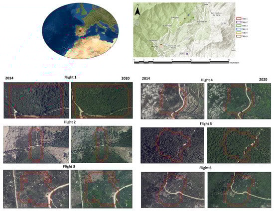
Figure 1.
Location of the sites where different flights were carried out. In the left panels the orthophotos are shown of the year corresponding to the first flight (2014) which was carried out at national level with low-density LiDAR data (0.5 points/m2); and in the right panels, the orthophotos (2020) closer to the second flights (2019) done with high-density LiDAR data (300 points/m2).

Table 1.
Main properties of the study areas (sites) according to the high-density LiDAR data (2019). Area in hectares (ha) and mean values and standard deviation of vegetation height (m), elevation (m), slope (degrees) and distance to nearest national geoid point (m) are given.
2.2. LiDAR Data
Low-density LiDAR data from the National Plan of Aerial Orthophotography (PNOA) was obtained from the 1st Spanish National LIDAR sites for the year 2014 and downloaded from the Spanish Geographic Institute (SGI) (http://centrodedescargas.cnig.es/CentroDescargas/index.jsp (accessed on 20 December 2021)). These LiDAR data were acquired with a Leica ALS60 Laser, which operated at a wavelength of 1064 nm and records up to four returns per pulse. The average point density was 0.5 points/m2 (including all returns), and the average point spacing was <1 m (Table 2) (for further details about LiDAR data see: http://pnoa.ign.es/especificaciones-tecnicas (accessed on 20 December 2021)).
Table 2.
Technical characteristics of sites and operation of the low-density LiDAR (PNOA) and high-density LiDAR (LidarPod) datasets.
High-density LiDAR data was obtained from the LIDAR device TerraSystem-LidarPod system formed by the Velodyne HDL-32e sensor (from now LidarPod) (https://www.routescene.com/ (accessed on 20 December 2021)) onboard of an unoccupied aerial vehicle (UAV). This system can obtain up to 700,000 points per second thanks to its 32 pairs of laser sensors. The density of points was around 300 points/m2 and the average point spacing was <0.05 m (Table 2). The equipment is complemented by a GNSS RTK system (real time kinematic: real-time position corrections) with accuracies of up to 1 cm, and an inertial navigation system (INS) that provides speed, acceleration and orientation. The LidarPod sites were carried out in six areas during 15–16 October 2019. The UAV used was a multirotor (Matrice 600 PRO). The flights were made at 5–7 m/s, 50 m height and in parallel lines separated by 40 m with an overlap greater than 50% (Table 2). Further technical details for each flight are given in Table S1.
2.3. LiDAR Processing
Errors in the vertical and horizontal accuracy of survey instruments were corrected by an automated boresight calibration method using a Bayesian multi-strip adjustment implemented in BayesStripAlign software (http://bayesmap.com/products/bayesstripalign/ (accessed on 20 December 2021)) [58]. To eliminate the boresight misalignment in the benchmark high-density LiDAR, time-tagged LiDAR point cloud, navigation data (trajectory position) and the position and orientation information for each pulse were used. This calibration method can compensate the time-varying boresight errors coming from the IMU, by working locally and directly from the site lines and removing corduroy artifacts (vertical bands) due to noise on attitude angles. The method uses all the strips at once in a Bayesian framework and directly computes the probability density function of the boresight angles [58,59]. Main corrections in XYZ and residual mean errors (RME) after correction are given in Table 3 and visual checking of the correction is shown in Figure S1. According to the vendor, the absolute vertical accuracy of low-density LiDAR data (PNOA) was around 15–40 cm based on real time kinematic (RTK) global positioning system (GPS) points [60].
Table 3.
Boresight calibration of high-density LiDAR data by using BayesStripAlign software (http://bayesmap.com/products/bayesstripalign/ (accessed on 20 December 2021)). Mean global corrections and residual mean errors (RME) after correction are given.
After boresight calibration, LiDAR data was preprocessed using LasTools software [36]: (i) removing replicated points (lasduplicate); (ii) filtering LiDAR points for noise (lasnoise) and (iii) transforming the altimetric datum (from ellipsoidal to orthometric) (lasheight using the options: -all_ground_points and -replace_z). Afterwards, last returns were classified into ground and no-ground classes using different classification filters (Figure 2): (i) the progressive triangulated irregular network (TIN) that it is a densification filter based on the method proposed by Axelsson [35], (ii) the progressive morphological filter (PMF), a morphological filter developed by Zhang et al. [38]; and (iii) the cloth simulation filter (CSF) that is a segmentation filter developed by Zhang et al. [39]. On the other hand, the low-density LiDAR files were previously classified by the vendor; and this filter was called “original”. This classification filter was only used for visual comparisons because the vendor did not explicitly indicate the filter used.
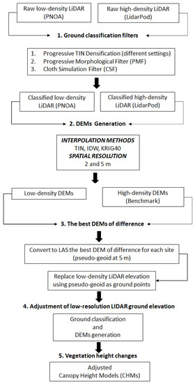
Figure 2.
Flowchart of the methodology followed to adjust low-density LiDAR ground elevation to benchmark high-density LiDAR data.
The progressive TIN densification filter was implemented using lasground tool in LasTools software. The parameterization of this tool consisted of the selection of two settings: (a) the terrain type, that was modulated by two step sizes (3 m (-wilderness) and 5 m (-default)) and (b) the granularity, i.e., how much computational effort to invest into finding the initial ground estimate using the switch “-hyper_fine”. Moreover, we fine-tuned the filter by specifying: (a) different thresholds at which spikes are removed from the ground: 0.5 and 3 m, (b) the maximal offset up to which points above the current ground estimate are included: 0.2 m; and (c) the bulge, a parameter specifying how much the TIN is allowed to bump (0.5 m and 3 m) (Table 4). The progressive morphological filter (PMF) and the cloth simulation filter (CSF) were implemented in the lidR package [61] of RStudio software [62]. In the case of the PMF filter, we used the settings proposed by Zhang et al. [39]: (a) ws: is the sequence of the size of the windows (in meters) used to filter the ground point returns (seq (3, 12, 4)); and (b) th: is the sequence of the threshold of heights above the ground surface over which a ground return is considered (seq (0.1, 1.5, length.out = length (ws)).
Table 4.
Settings of the progressive TIN densification filter used in LasTools software. The setting called Siose Forest (SF) came from the methodology followed to classify low-resolution LiDAR (PNOA) in the Spanish region of La Rioja (https://www.iderioja.larioja.org/ (accessed on 21 December 2021)).
Once the LiDAR point clouds were classified into ground and non-ground using the different filters and settings, DEMs derived from different interpolation methods at 2 m and 5 m pixel size were generated from the ground returns (Figure 2). To carried out this task, we used the lidR package [61] in RStudio applying the Grid Terrain function and selected three types of interpolation: (i) TIN: based on Delaunay triangulation; (ii) knnidw: based on the distance to the nearest neighbor (KNN) with an inverse distance weighting (IDW) and (iii) Kriging: function combining the KNN approach and the Kriging approach (based on spatial correlation). Finally, we built the canopy height models (CHMs), selecting the better spatial resolution from the DEM of difference with the lowest vertical errors, using a “spike-free” algorithm [63] (Figure 2). This method resolves the problem of the empty pixels and so-called “pits” by the interpolation of first returns with a TIN and then, rasterizing it onto a grid. It consisted of several layers of triangulation at different height bins (at 0, 2, 5, 10, 15, 20 and 30 m). Moreover, the pit-free algorithm combined with the subcircling tweak which replaces each return by a circle with a small radius (i.e., option “-subcircle 0.25”) worked adequately without empty pixels or pits. This algorithm was implemented in LidR package in RStudio using the function “grid_canopy”.
2.4. DEMs of Difference: Correction of Low-Density LiDAR Ground Elevation
To correct ground elevation of low-density LiDAR, we took the high-density LiDAR dataset (Figure 2) as the benchmark. We made differences between pairs of DEMs (low- vs. high-density) for all methods (classification filters, interpolation methods and spatial resolutions) and selected the one with the lowest differences (i.e. the best DEM of difference). This approach worked like the standard method for converting ellipsoidal heights to orthometric ones using the geoid and it was adapted to the specific site-conditions of each environment. The elevation differences were used to replace the elevation values of low-density LiDAR using the lasheight function with the following parameters: “-all_ground_points” and “-replace-z” in LasTools. Positive values in elevation differences indicated that the surface derived from the low-density LiDAR was higher than the benchmark elevation and then, over-predicted it, whereas negative values indicated the opposite. As pointed out by Zandberger [64], errors in DEMs are often not normally distributed. Therefore, we checked for non-normality by using quantile-quantile (Q-Q) graphs and calculating robust accuracy measures for non-normal distributions [65]: (i) the 50% quantile (P50) of the errors that is a robust estimator for a systematic shift of DEMs; (ii) the normalized median absolute deviation (NMAD) (Equation (1)) that is a robust estimator, resilient to outliers in DEMs; and (iii) the root mean square error (RMSE) that indicates on average how far observed values differ from the benchmark values [66].
where denotes the individual errors j = 1,…, n and is the median of the errors (P50) [65].
2.5. Factors Influencing DEMs Accuracy
To assess if there were significant differences among the residual DEMs using different classification filters, interpolations and resolutions, factorial ANOVA (analysis of variance) was applied. In the factorial ANOVA, the response variables were the P50, the NMDA and the RMSE of each residual DEM and the explanatory ones were site, classification filter, interpolation method and spatial resolution. Later, the Kruskal–Wallis and Dunn tests were used to assess which factors individually and combined, were significant in explaining the differences among DEMs.
Moreover, to assess how site-specific factors (i.e., topographic features (elevation and slope), vegetation height, and distance to the nearest geoid point) significantly explained the vertical errors of low-density LiDAR derived DEMs, generalized additive models (GAMs) (with linear terms) were carried out. We randomly sampled the study areas using 20 m as minimum distance between points to avoid autocorrelation and extracted elevation differences and the values of the explanatory variables (the number of sampling points ranged from 25 to 50 depending on the size of the sites). To assess the consistency of the relationships, several GAMs were run at different levels of data aggregation: (i) a global multivariate GAM including all explanatory variables and using the sampling points of all sites and their replications by the different classification filters (the interpolation method (TIN) and the spatial resolution (5 m) were kept fixed); (ii) univariate GAMs (including only one explanatory variable) for each site using the replicated sampling points from the different classification filters and, (iii) multivariate GAMs for each classification filter within each site. For estimating distance to the nearest geoid point, the national geoid model “EGM08-REDNAP” was downloaded from the geodesy area of the SGI (https://www.ign.es/web/ign/portal/gds-area-geodesia (accessed on 21 December 2021)). The EGM08-REDNAP provides points at 1′ × 1′ (1′ = 1.85 km) distant, that collect the geoid ondulation, that is the deviation from the vertical (difference between the height of the geoid and the ellipsoid (https://www.ign.es/web/ign/portal/gds-area-geodesia (accessed on 21 December 2021)). Finally, we used GAMs to assess if vertical errors could influence the vegetation height changes observed between dates (2014–2019).
3. Results
The Q-Q plots of the elevation differences between low-and high-dense LiDAR derived DEMs showed that vertical errors in each site followed a non-normal distribution (Figure S2). Accordingly, the RMSE overestimated the vertical error, whereas the 50th percentile (P50), underestimated it; the NMDA being more appropriate for being resilient to outliers in DEMs [65]. Factorial ANOVA indicated that there were significant differences in elevation errors among sites (93% of the variance in residual heights was explained by sites (not shown)); and according to the NMDA and RMSE, among classification filters values too (the CSF filter was significant different of the rest showing the highest error) (Table 5). On the contrary, there were not significant differences in vertical errors aggregating by the interpolation method or the spatial resolution. When vertical errors were analyzed within each site, significant differences among classification filters were found but not among interpolation methods or spatial resolutions (Tables S2–S4). The greatest errors were in site 1 using the CSF filter (P50: −2.38 m; NMDA: 1.07 m and RMSE: 3.19 m) and the lowest ones in site 2 using the TIN-SW2 filter (P50: 0.01 m; NMDA: 0.28 m and RMSE: 0.41 m) (Tables S2–S4).
Table 5.
Mean and standard deviation of the uncorrected elevation differences between low- and high-density LiDAR datasets (i.e., DEMs of difference) measured by the 50th percentile (P50), the normalized median absolute deviation (NMAD) and the root mean square error (RMSE) grouping by sites (sites), classification filters, interpolation methods and spatial resolutions. Letters indicate significant differences within groups according to the post-hoc Dunn´s non-parametric test for Kruskal-type ranked data with a significance level of p < 0.05.
Visually checking the DEMs hillshades, we assessed that the TIN densification algorithms using default parameters (DEF) or low spikes (0.5) (SF, SW2) were smoother (Figure 3 and Figure S3) showing lower vertical errors (Table 5) whereas the CSF and the TIN densification algorithms using large spike (3) (i.e., WILD), followed by the morphological filter (PMF), showed a lot of bumps and spikes (Figure 3 and Figure S3); and also, high elevation differences (Table 5).
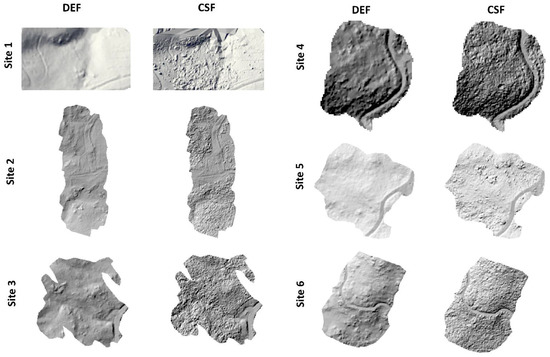
Figure 3.
Hillshades from DEMs (at 1 m pixel size for better interpretation) derived from high-density LiDAR data using TIN densification with default parameters (DEF) and the segmentation-based filtering, the “Cloth Simulation Filter” (CSF).
After subtracting the elevation differences to the raw low-density LiDAR data using the best method (with the lowest vertical errors), a good adjustment was obtained (Figure 4). Histograms of elevation differences before and after correction for each site using the best method are shown in Figure S4. In addition, visual checking of the corrected hillshades allowed assessing of the qualitative improvement in respect to the hillshades derived from the original ground classification of low-density LiDAR data (Figure 5). Furthermore, a cluster analysis on uncorrected and corrected elevation values using the k-means algorithm and the Dunn´s non-parametric test for Kruskal-type ranked data confirmed the significant effects of the correction of raw low-density LiDAR elevation data (Figure S5).
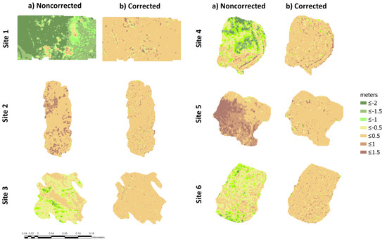
Figure 4.
Elevation differences (in meters) before (a) and after (b) correction using the best classification filter. In sites 1, 4 and 6: TIN densification algorithm with Siose Forest settings (TIN-SF); in site 2, the progressive morphological filter (PMF) and in sites 3 and 5, the TIN densification algorithm with default settings (DEF). For all sites, the TIN interpolation method and 5 m spatial resolution was kept constant. Maps are shown at 2 m spatial resolution for better interpretation.
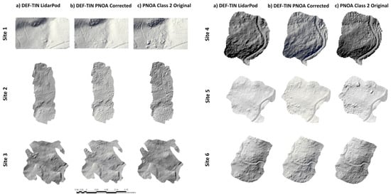
Figure 5.
Hillshades of DEMs using the TIN densification filter with default parameters (DEF) (at 1 m pixel size for better interpretation) from: (a) high-density LiDAR; (b) corrected low-density LiDAR and (c) uncorrected low-density LiDAR using the original classification filter.
The corrected P50 ranged from −0.004 to −0.016 m, the NMDA from 0.06 to 0.10 m and the RMSE from 0.28 to 0.46 m, aggregating by sites (Table 6). The corrected P50 did not show significant differences among sites, classification filters, interpolation methods or spatial resolutions. However, the corrected NMDA and RMSE indicated that the CSF filter algorithm, the spatial resolution at 2 m and the IDW interpolation method, this latter only in accordance with the NMDA, showed the greatest errors (Table 6). Moreover, factorial ANOVA within each site showed significant differences among interpolation methods and spatial resolutions. The greatest errors continued in site 1 using the CSF filter (P50: −0.091 m; NMDA: 0.14 m and RMSE: 0.69 m) and the lowest ones in site 3 using the TIN-DEF filter (P50: −0.001 m; NMDA: 0.04 m and RMSE: 0.09 m). Overall, the TIN densification filters with low spikes (SF, SW2) and default settings (DEF) showed the lowest errors as well as the Kriging interpolation method and the spatial resolution of DEMs at 5 m (Tables S5–S7).
Table 6.
Mean and standard deviation of corrected elevation errors (i.e., DEMs of differences) measured by the 50th percentile (P50), the normalized median absolute deviation (NMAD) and the root mean square error (RMSE) grouping by sites (sites), classification filters, interpolation methods and spatial resolutions. Letters indicated significant differences within groups according to the post hoc Dunn´s non-parametric test for Kruskal-type ranked data with a significance level of p < 0.05.
To explain vertical errors from site-factors, GAMs (with linear terms) at different levels of aggregation were carried out. The global multivariate GAM including all sites and classification filters explained ca. 47% of total deviance (Table 7). The slope and the distance to the nearest geoid point were the most important explanatory variables. Overall, as the slope increased, the elevation residuals were more negative (underestimation of benchmark elevations) whereas as the distance to the nearest geoid point increased, the elevation residuals were more positive (overestimation of benchmark elevations) (Figure 6). Univariate GAMs for each site including all filters indicated that the distance to the nearest geoid point was the best explanatory variable for all sites, except for sites 2 and 6 that were poorly explained by the site conditions (Table 8). Finally, multivariate GAMs for each classification filter within each site indicated that vertical errors in sites 1 and 4 were better explained by site factors than those in the other sites (deviance explained 40% ± 0.07 and 57% ± 0.07, respectively) as well as the TIN densification filter with default settings (DEF) and the PMF filter. Nevertheless, all these GAMs showed low fitting ability (from 13% to 57% of deviance explained) (Tables S8–S13).
Table 7.
Results of the global multivariate GAM (with linear terms) using as response variable the vertical errors of DEMs derived from different classification filters in all sites using the TIN interpolation method at 5 m pixel size; and as explanatory ones: site-specific factors (i.e., elevation, slope, vegetation height and distance to nearest geoid point). Coefficients of main explanatory variables (all significant with a p < 0.05, except the intercept), and global and partial adjusted R2 and explained deviance of GAMs are given.
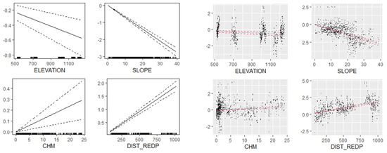
Figure 6.
Plots of partial relationships between the vertical errors of DEMs (y axes) derived from low-density LiDAR and site-specific factors (x axes). Estimations are derived from the global multivariate GAM that included all sites and all classification filters. From left to right: elevation, slope, vegetation height (CHM: canopy height model) and distance to the nearest geoid point (DIST_REDP).
Table 8.
Univariate generalized additive models (GAMs) of each site-specific factor to estimate their relative importance in explaining the vertical errors of DEMs derived from low-density LiDAR. The response variable is the vertical error of each site. All classification filters are included maintaining the interpolation method (TIN) and the spatial resolution (5 m).
Finally, we assessed if changes in vegetation height could be related to the vertical errors found before correction. The results of this analysis indicated that changes in vegetation height were decoupled from elevation vertical errors in nearly all sites (Tables S14 and S15). Nevertheless, we found a significant relationship in site 4 and in site 6 (Figures S6 and S7). In those cases, there was a positive relationship indicating that sampling points with large negative vertical error had the lower vegetation height changes, and points with lower elevation errors (less negative or positive) had larger vegetation height changes. As preliminary results, we observed that from 2014 to 2019, the greatest vegetation height increases occurred in site 1 (+3.9 m on average), followed by site 3 (+3.0 m) and 2 and 4 (ca. +2.0 m). The lowest increases were found in site 6 (+1.33 m) and site 5 (+0.4 m) on average (Figure 7).
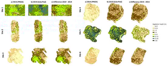
Figure 7.
Canopy height models (CHMs) from: (a) low-density LiDAR (2014), (b) high-density LiDAR (2019) and (c) their height differences for each site using the best classification filter: In sites 1, 4 and 6: TIN densification algorithm with Siose Forest settings (SF); in site 2, the progressive morphological filter (PMF) and in sites 3 and 5, the TIN densification algorithm with default settings (DEF).
Quantitative assessment of vegetation changes by repeated LiDAR data is a challenge because it requires producing reliable change maps that are robust to differences in survey conditions, free of processing artifacts, and that consider various sources of uncertainty, such as different point densities, georeferencing errors and geometric discrepancies [58,59]. Here, the raw elevation of low-density LiDAR was adjusted to the elevation of high-density LiDAR using the best DEM of difference as local pseudo-geoid (i.e., all interpolated points). This approach improved the vertical accuracy of the target DEMs, minimized the random nature of vertical errors and decoupled vegetation changes from ground elevation errors.
4. Discussion
The first step before comparing low- and high-density LiDAR datasets was to assure that there were no systematic or instrumental errors in data collection [15]. The calibration method to eliminate boresight misalignment in the benchmark high-density LiDAR ensured high internal vertical and horizontal consistency (1–6 cm of error in XYZ) and the vertical accuracy given by the vendor was around 3–6 cm. In addition, low-density LiDAR strips were aligned using GNSS ground checking points, and the vertical accuracy was 15–20 cm. Main differences in vertical accuracy of both LiDAR data sets can be attributed to the greater beam size and less sensitivity of the laser as site altitude increases. For example, Hyyppä et al. [17], who used data collected in three separate sites, observed that the increase of site altitude from 400 to 1500 m increased the random error of DEM derivation by 50%. This was mainly due to the decrease of the pulse density and increase in the planimetric error (for non-flat surface).
Nevertheless, DEM derived from low-density LiDAR data (ca. 1 point/m2 in our case) is hampered by poor quality of ground returns [10,14,32,67]. Accordingly, the adjustment of low-density LiDAR elevation with respect to a benchmark with higher point density is recommended [7]. James et al. [11] demonstrated that extracting control points from high-density LiDAR derived DEM can produce a photogrammetric DEM of comparable quality to that achieved with high accurate ground checkpoints. However, to achieve such positive results, it is important to choose suitable control points and to ensure that change between epochs is minimal [11]. Moreover, the inadequate quantity and spatial distribution of GCPs will in turn degrade the accuracy of DEM products [9]. In this sense, other studies assessed certain limitations in correcting less accurate DEMs (i.e., SRTM DEM) by applying regression models using checkpoints from LiDAR data [12,13]. For example, Su and Guo [12] observed that, although vertical errors decreased (from over 12 to −0.8 m) after correction, large errors continued by using the regression model. Likely, Su et al. [13] following the same methodology assessed that the corrected SRTM DEM continued being about 2.5 m lower than the GLAS elevation on average. These results might indicate that the random nature of elevation errors can limit the usefulness of elevation corrections from regression analysis based on some checkpoints and their properties.
Here, we corrected elevation data from low-density LiDAR (1 point/m2 on average taken at 3000 m of site height) to high-density LiDAR elevation data (300 points/m2 on average and taken at 50 m of site height) using the entire grid of interpolated elevation differences as true checkpoints with respect to the high-density LiDAR instead of only some control points. By significantly increasing the number of checkpoints used in the adjustment, the redundancy produced better results than using an inferior number of ground control points [11]. Moreover, by means of the DEMs of difference, we conformed high dense surfaces of elevation deviations (i.e., dense local “pseudo-geoids”) that served to adjust the raw elevation of low-density LiDAR points to the benchmark ones giving a straightforward quantitative control test whereby differences closest to zero represented the best quality DEM surfaces [4,8,9].
However, before making such elevation corrections, a previous checking of the effect of the classification filters, the interpolation methods and the spatial resolution on the vertical errors of DEMs is required. It has been shown that the quality of a DEM is dependent on a correct classification of these points as ground [3,23]. The performance of the classification filters differs under different LiDAR point density as well as terrain and vegetation conditions [2,34,35,68]. Moreover, there is little guidance in the literature regarding the selection of parameters to optimize filtering [37]. Accordingly, due to the lack of optimal classification filters, quality control becomes necessary to select the most suitable in each context [31].
We observed large differences in vertical errors among classification filters. As the Q-Q plots showed that vertical errors in each site followed a non-normal distribution, the NMDA, resilient to outliers, was used to report more appropriate vertical errors in DEMs [65]. Before correction, and according to all error metrics, the CSF and the TIN-WILD filters showed significant higher vertical errors than TIN-DEF, TIN-SW2 and TIN-SF in all sites. After correction, the vertical errors dropped significantly. The NMDA ranged from 0.14 (site 1 using CSF filter) to <0.06 m (in all sites and all classification filters except the CSF and TIN-WILD). These errors were within the accuracy specifications of low-density LiDAR data given by the vendor (0.15–0.20 m). Moreover, a detailed visual analysis of DEMs of difference after correction revealed that vertical errors were more randomly distributed although reflecting some artefacts derived from the used classification filter [47,48].
The TIN densification filter with “Default” settings (DEF) or low spikes (i.e., SW2 and SF) for both LiDAR datasets drew smoother DEMs whereas the segmented-based (CSF) filter and TIN densification one using large spikes (i.e., WILD) showed many artifacts as bumps and peaks. CSF and TIN-WILD erroneously included low and dense vegetation as ground (type II error) but drew cliffs and steep slopes perfectly (see Viedma et al. [68] for further details). On the contrary, TIN densification filters using low spikes (TIN -DEF, -SW2 and -SF) correctly classified understory or low/dense shrubs as non-ground but resulted in several ground classification errors in steep slopes, cliffs and deeply incised stream banks (type I error) [68,69]. In this way, as none of them worked perfectly, and all methods are susceptible to both omission and commission errors, users might consider testing different classification filters to avoid unpredictable results [30] and the possibility of combining multiple classification procedures to exploit the strengths of each other [68,69]. For example, Viedma et al. [68] combined different classification filters to estimate low (<2 m) and high (>2 m) vegetation in a very complex terrain in eastern Spain, removing type I and II errors.
Besides the effects of the classification filters on vertical accuracy of DEMs, the interpolation from points onto a grid can also introduce a degree of uncertainty into the DEMs [6,10,28]. Here, we asserted that before correction there were not significant differences on vertical errors due to the interpolation method neither among nor within sites (even by controlling the filter classification in the ANOVA (not shown here)). Nevertheless, after correction, and according to the NMDA, the vertical errors were significantly lower using the Kriging method than using the IDW in all sites. It has been observed that the vertical errors in DEMs are more dependent on the choice of interpolation method for low points density than for high sampling density [67]. At lower sampling densities, Kriging yielded the best elevation estimations improving IDW (inverse distance weighted) [5,8,13,27,67,70]. However, if sampling data density is high, the IDW method performs well [10,42,67]. Moreover, Yilmaz and Uysal [18] found that the TIN interpolation was superior to other interpolation methods with the lowest RMSE. According to these results, it is evident that these interpolation methods are suitable for some specific conditions, and their general applicability is limited; there still being a lack of consensus about which interpolation method is most appropriate for the different terrain data. None of the interpolation methods is universal for all kinds of data sources, terrain patterns or purposes [18,42].
Furthermore, we found that there were not significant differences on vertical errors due to the spatial resolution of DEMs. Before correction, none of the error metrics showed significant differences in relation to the spatial resolution neither among nor within sites (even by separating/controlling the filter classification in the ANOVA (not shown here)). However, after correction, NMDA, followed by the P50 and RMSE, indicated that the larger the pixel size was, the lower the vertical error. It was expected that the most accurate surfaces were created using grids which had a similar spacing to the original points (ca. 2 m) [10,46]. However, Guo et al. [27] showed that DEMs at high resolutions (0.5 and 1 m) produced relatively higher RMSE than DEMs at lower resolution (5 and 10 m), mainly by the smooth effect of large pixel size.
On the other hand, the vertical accuracy of the DEMs is affected by site conditions (mainly vegetation and terrain morphological characteristics) [3,4,5,17,22,33,49,50,51]. In relation to the effects of vegetation, we showed that vertical errors in DEMs were low and explained by vegetation height (CHM); reaching a maximum ca. 10% of deviance explained in some sites. However, despite the low explanatory power of this factor, vertical errors increased significantly with vegetation height favoring the overestimation of benchmark elevations. These results agreed with other ones finding positive elevation bias in high vegetated areas and negative bias in open vegetation and agricultural land covers [7,9,11,13,53,66,71]. Nevertheless, other studies found the opposite [12,23,68]. For example, Chaplot et al. [67] observed that elevations were overpredicted (6.0 cm) in open vegetated areas and underpredicted (−3.8 to −6.0 cm) in brush low/trees and evergreen forests. Likely, Su and Guo [12] assessed that the percentage of pixels with negative difference increases to nearly 100% in the group with the maximum vegetation height at all study sites. Finally, others have not found any relationship [2,8,33]. In the case of Hodgson et al. [32], it was found that LiDAR derived elevation was significantly underpredicted in all studied land cover classes; although the underprediction was largest in pine forest areas, by up to 0.24 m.
Regarding the effects of terrain complexity on vertical accuracy of DEMs, it has been shown that slopes, roughness or topographic variability (closely related to slope) contribute significantly to the errors of DEMs [2,14,17,23,28]. For example, Razak et al. [51] observed that DEM errors in slopes over 40° were significantly higher than the overall RMSE (1.53 m vs. 0.89 m). Tinkham et al. [2], reported that the vertical error increased on slopes exceeding 30° and Hodgson and Bresnahan [23] that the elevation error in slopes about 25° was twice those in flatter slopes (1.5°). Finally, Mukherjee et al. [66] showed that significant impacts occurred only with slopes above 10° on ASTER and SRTM DEMs accuracy. On the contrary, Su et al. [13] showed that, compared to the influence of vegetation, slope had no significant influence on the mean difference between the SRTM DEM and the LiDAR DEM. Likely, Hodgson et al. [32] reported that, except for low grass, none of the other land cover categories exhibited a statistically significant relationship between LiDAR elevation errors and terrain slope. Here, terrain slope was the best predictor of vertical errors among sites explaining ca. 28% of total deviance but this effect was lower within sites. These results could be explained by the wide range of slope variability (0 to 40°) covered among sites and the low range of variability within them. Consistently, higher slopes increased vertical errors and underpredicted benchmark LiDAR elevations (negative elevation differences).
In addition, we included as site-specific variable, the distance to the nearest geoid point. This variable was never analyzed in previous studies and resulted in high explanatory power (24.3% of total deviance), following the slope. Results indicated that increasing the distance to the nearest geoid points, the greater the positive vertical error (overprediction of benchmark elevation). For example, Daniels [72] observed that the elevation difference between the ellipsoidal heights and the orthometric ones increased as one travels north from the Columbia River toward Washington. This regional trend implied that the use of an orthometric height correction factor calculated for the base station alone will not correct all offsets in the data, and that the correction factor required may vary based on the location of the LIDAR instrument in relation to the base station.
Finally, we assessed that changes in vegetation height were decoupled from elevation vertical errors. The significant relationship observed in some sites did not explain casualty; mainly because we expected similar vertical errors in DEMs and CHMs after correction; and in all cases, height differences were significantly larger than elevation errors; agreeing with the results obtained by Dubayah et al. [73]. Finally, and as preliminary results, we quantified an average annual growth of 0.39 ± 0.24 m/y that ranged from 0.13 (in site 5) to 0.87 m/y (in site 1) for 5 years (2014–2019). These different growth rates could be related to the age of vegetation, assuming that younger trees had a faster growth rate than older ones (site 1 was composed by trees burned in 1990 and site 5 by older trees never burned in the last 40 years). For example, Vepakomma et al. [74], using multitemporal LiDAR, showed that younger trees (ca. 10–15 m) grew ca. 2 m in 5 years (0.5 m/y) whereas the older ones (>15 m) around 0.4 m (0.08 m/y) in Canada. Conversely, others have found larger growth rates in old forests using repeated LiDAR. For example, Englhart et al. [75] quantified a tree height increase of 2.3 m in 4 years (ca. 0.6 m/y) in unaffected forests and Hopkinson et al. [76] an annual growth of 0.5 m/y in a red pine planation in Canada. Moreover, Hudak et al. [77] reported even larger annual growth (0.8 m/y) in a mixed-conifer forest in the US. These large height changes could be attributed to the way conifers trees grow. Conifer trees grew by elongating their tips vertically, and by elongating existing branches horizontally [74]. Accordingly, points that have hit on low surfaces near the crown borders during the first LiDAR survey will be much higher in the last one as the result of hitting on the crown due to lateral growth (Figure 8). These results indicated that changes in canopy architecture over time are also important.
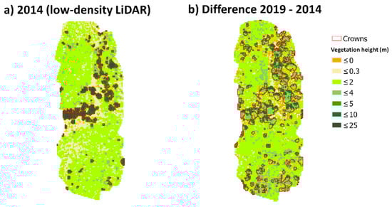
Figure 8.
Canopy height models (CHMs) derived from (a) low-density LiDAR data (2014) and (b) the difference between low- and high-density LiDAR derived CHMs. In red, the crowns shapes identified in low-density LiDAR (a) and those from the high-density LiDAR dataset (b).
On the other hand, it has been reported that low-density LiDAR showed a noticeable underestimation bias of trees height [78,79]. For example, Zhao et al. [79] quantified a bias of −1.5 m (n = 598) in respect to field data mainly due to the increased probability of missing treetops as pulse density decreases. Here, we show, as an example, the cloud of points of some “supra crowns” to visually assess the canopy differences between low- and high-density LiDAR datasets (Figure 9).
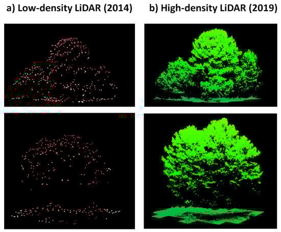
Figure 9.
Snapshots of “supra-crowns” derived from (a) low-density LiDAR (2014) and (b) high-density LiDAR (2019).
As future work, several issues need to be resolved for improving the estimation of vegetation growth from repeated LiDAR with different point densities: (i) a more robust comparison of vegetation height changes from low- and high-density LiDAR datasets, (ii) unmixing the effects of vertical and lateral growth and (iii) to develop robust models between field growth measures (for example, from multitemporal national forest inventories) and observed LiDAR values. In relation to a reliable comparison between low- and high-density LiDAR datasets, we could apply the approach proposed by Zhao et al. [79] who corrected the relative biases of low-density LiDAR measured tree heights using the LiDAR data with the highest laser pulse rate and thinning it at a series of lower point densities. This approach built a regression model whose coefficients were used to correct tree heights derived from low-density LiDAR. In addition, to guarantee the comparability of forest metrics from low- and high-density LiDAR surveys, area-based LiDAR metrics will be applied for being more reliable in estimating forest metrics [79,80,81]. Compared to individual tree analyses, area-based analysis is less affected by the inconsistencies between low- and high-density LiDAR data to measure forest dynamics; and allow the classification the spatiotemporal patterns of forest changes [79]. To unmix the effects of vertical and lateral growth, height measures will consider only the common crown section, giving more accurate height changes; and finally, to assure the robustness of the relationship with ground data; separated LiDAR models for each LiDAR survey with temporally coincident ground data can counteract the inconsistency in repeat LiDAR data with different point densities [2,75].
5. Conclusions
Standardization of ground elevation is obligatory for comparison of LiDAR derived forest metrics at different dates. After standardization, it can be reasonably assumed that the relative accuracy between CHMs is like the DEM accuracy. In this paper, it has been assessed that although high-density LiDAR data does not provide a perfect elevation model, it was considerably more accurate compared to low-density LiDAR; and therefore, it was a good benchmark. Our approach was novel mainly because continuous surfaces of elevation differences, instead of a collection of checkpoints, were used to correct the raw elevation of low-density LiDAR. Moreover, using the “best DEM of difference” approach, based on comparing the vertical errors raised from different methodologies (i.e., classification filters, interpolation methods and spatial resolutions), the elevation of each site was more accurately corrected reducing random or methodological errors that would be very difficult to correct by using only checkpoints.
Overall, it was observed that the classification filters based on TIN densification algorithm using default parameters or low spikes (TIN-DEF or TIN-SF), the Kriging interpolation method and 5 m pixel size adequately corrected elevation deviations in all sites. After correction, vertical errors declined drastically, reaching low values (from 0.04 to 0.08 m) using the best DEM of difference in each site. Nevertheless, none of the classification filters worked perfectly in each site, and all of them are susceptible to both omission and commission errors. Accordingly, the possibility of combining different classification filters in the same environment is recommended to exploit the strengths of each other. On the other hand, the vertical errors observed between low- and high-density LiDAR datasets were partially explained by site factors (maximum deviance explained was 57% ± 0.07). The slope and the distance to the nearest geoid point were the most important explanatory variables. Overall, the higher the terrain slope and the distance to the nearest geoid, the higher the vertical errors. Vegetation height played a minor role, but vertical errors increased significantly with vegetation height. Finally, we assessed that changes in vegetation height were decoupled from elevation vertical errors at all sites.
The findings of the study are important to understand the sources of DEMs error by analyzing the role of methodological and site-specific factors; and also, to correct vertical errors of low-density LiDAR derived DEMs by using “the best DEM of difference” method. This approach considerably reduced the effects of elevation errors on vegetation height changes. The study recommends that, before comparing LiDAR datasets with different point densities, “the best DEM of difference” should be considered for correcting the target elevation dataset; mainly because each environment has its own physical properties, and this method allows adapting of the best DEM to each site. Finally, the estimation of vegetation growth from repeated LiDAR with different point densities must be improved, requiring further studies.
Supplementary Materials
The following supporting information can be downloaded at: https://www.mdpi.com/article/10.3390/f13030380/s1. Table S1: Technical characteristics of LiDAR datasets; Tables S2–S4: Mean and standard deviation of uncorrected elevation errors (i.e., DEMs of differences) measured by the percentile 50th, NMDA and RMSE, respectively; Tables S5–S7: Mean and standard deviation of corrected elevation errors (i.e., DEMs of differences) measured by the percentile 50th, NMDA and RMSE, respectively; Tables S8–S13: GAMs (with linear terms) for each site using as response variable the uncorrected vertical errors derived from the CSF, TIN-DEF, PMF, TIN-SF, TIN-SW2 and TIN-WILD classification filters and as explanatory ones the site conditions; Table S14: Estimated coefficients of the vertical errors of DEMs in GAMs for explaining the corrected vegetation height changes (2014–2019); Table S15: The percentage of deviance in the corrected vegetation height changes (2014–2019) explained by the vertical errors of DEMs. Figure S1: Clouds of points from high-density LiDAR data before (left panel) and after (right panel) correction of the boresight misalignment; Figure S2: Normal Q-Q graph for the distribution of the uncorrected elevation differences; Figure S3: Hillshades of DEMs derived from high-density LiDAR data using different classification filters; Figure S4: Histograms of the elevation differences between low- and high-density DEMs before and after correction; Figure S5: Cluster K-means of the elevation differences between low- and high-density LiDAR derived DEMs before and after correction; Figures S6 and S7: Scatterplots of the relationship between the vegetation height changes (2014–2019) occurred in site 4 and the vertical errors of the DEM built using the TIN-SF and the TIN-SW2 classification filters, respectively.
Funding
This research was part of the INFORICAM project funded by MCIN/AEI/10.13039/501100011033/ and by “European Union NextGenerationEU/PRTR”. Grant number PID2020-119402RB-I00.
Institutional Review Board Statement
Not applicable.
Informed Consent Statement
Not applicable.
Data Availability Statement
Available under request.
Acknowledgments
The support given by the Spanish Agencia Estatal de Investigación (AEI) and the Ministerio de Ciencia e Innovación (MCIN) as well as the European funding (European Union NextGenerationEU/PRTR) (project PID2020-119402RB-I00) is acknowledged. I thank Danilo R. Almeida, Jose Manuel Moreno Rodriguez, and Natalia Quintero Ñustez for their helpful comments and support. I highly appreciate the work of the reviewers for their valuable input to this submission.
Conflicts of Interest
The author declares no conflict of interest. The funders had no role in the design of the study; in the collection, analyses, or interpretation of data; in the writing of the manuscript, or in the decision to publish the results.
References
- Clark, M.L.; Clark, D.B.; Roberts, D.A. Small-footprint lidar estimation of sub-canopy elevation and tree height in a tropical rain forest landscape. Remote Sens. Environ. 2004, 91, 68–89. [Google Scholar] [CrossRef]
- Tinkham, W.T.; Smith, A.M.S.; Hoffman, C.; Hudak, A.T.; Falkowski, M.J.; Swanson, M.E.; Gessler, P.E. Investigating the influence of LiDAR ground surface errors on the utility of derived forest inventories. Can. J. For. Res. 2012, 42, 413–422. [Google Scholar] [CrossRef]
- Hansen, E.H.; Gobakken, T.; Næsset, E. Effects of pulse density on digital terrain models and canopy metrics using airborne laser scanning in a tropical rainforest. Remote Sens. 2015, 7, 8453–8468. [Google Scholar] [CrossRef] [Green Version]
- Simpson, J.E.; Smith, T.E.L.; Wooster, M.J. Assessment of errors caused by forest vegetation structure in airborne LiDAR-derived DTMs. Remote Sens. 2017, 9, 1101. [Google Scholar] [CrossRef] [Green Version]
- Salekin, S.; Burgess, J.H.; Morgenroth, J.; Mason, E.G.; Meason, D.F. A comparative study of three non-geostatistical methods for optimising digital elevation model interpolation. ISPRS Int. J. Geo-Inf. 2018, 7, 300. [Google Scholar] [CrossRef] [Green Version]
- Smith, S.; Holland, D.; Longley, P.A. The importance of understanding error in Lidar digital elevation. Int. Arch. Photogramm. Remote Sens. Spat. Inf. Sci. 2004, 35, 996–1001. [Google Scholar]
- Aguilar, F.J.; Mills, J.P.; Delgado, J.; Aguilar, M.A.; Negreiros, J.G.; Pérez, J.L. Modelling vertical error in LiDAR-derived digital elevation models. ISPRS J. Photogramm. Remote Sens. 2010, 65, 103–110. [Google Scholar] [CrossRef]
- Liu, X. Accuracy assessment of lidar elevation data using survey marks. Surv. Rev. 2011, 43, 80–93. [Google Scholar] [CrossRef] [Green Version]
- Barrand, N.E.; Murray, T.; James, T.D.; Barr, S.L.; Mills, J.P. Optimizing photogrammetric DEMs for glacier volume change assessment using laser-scanning derived ground-control points. J. Glaciol. 2009, 55, 106–116. [Google Scholar] [CrossRef] [Green Version]
- Liu, X.; Zhang, Z.; Peterson, J.; Chandra, S. The effect of LiDAR data density on DEM accuracy. In Proceedings of the MODSIM 2007-International Congress on Modelling and Simulation-Land, Water and Environmental Management: Integrated Systems for Sustainability, Christchurch, New Zealand, 10–13 December 2007; Modelling and Simulation Society of Australia and New Zealand Inc.: Christchurch, New Zealand, 2007; pp. 1363–1369. [Google Scholar]
- James, T.D.; Murray, T.; Barrand, N.E.; Barr, S.L. Extracting photogrammetric ground control from lidar DEMs for change detection. Photogramm. Rec. 2006, 21, 312–328. [Google Scholar] [CrossRef]
- Su, Y.; Guo, Q. A practical method for SRTM DEM correction over vegetated mountain areas. ISPRS J. Photogramm. Remote Sens. 2014, 87, 216–228. [Google Scholar] [CrossRef]
- Su, Y.; Guo, Q.; Ma, Q.; Li, W. SRTM DEM correction in vegetated mountain areas through the integration of spaceborne LiDAR, airborne LiDAR, and optical imagery. Remote Sens. 2015, 7, 11202–11225. [Google Scholar] [CrossRef] [Green Version]
- Williams, R. DEMs of Difference. Geomorphol. Tech. 2012, 2, 1–17. [Google Scholar]
- Latypov, D. Estimating relative lidar accuracy information from overlapping flight lines. ISPRS J. Photogramm. Remote Sens. 2002, 56, 236–245. [Google Scholar] [CrossRef]
- Reutebuch, S.E.; Mc Gaughey, R.J.; Andersen, H.E.; Carson, W.W. Accuracy of a high-resolution lidar terrain model under a conifer forest canopy. Can. J. Remote Sens. 2003, 29, 527–535. [Google Scholar] [CrossRef]
- Hyyppä, H.; Yu, X.; Hyyppä, J.; Kaartinen, H.; Kaasalainen, S.; Honkavaara, E.; Rönnholm, P. Factors affecting the quality of DTM generation in forested areas. Int. Arch. Photogramm. Remote Sens. Spat. Inf. Sci. 2005, 36, 85–90. [Google Scholar]
- Yilmaz, M.; Uysal, M. Comparison of data reduction algorithms for LiDAR-derived digital terrain model generalisation. Area 2016, 48, 521–532. [Google Scholar] [CrossRef]
- Baltsavias, E.P. Airborne laser scanning: Basic relations and formulas. ISPRS J. Photogramm. Remote Sens. 1999, 54, 199–214. [Google Scholar] [CrossRef]
- Pothou, A.; Toth, C.; Karamitsos, S.; Georgopoulos, A. On using QA/QC techniques for LiDAR-IMU boresight misalignment. Int. Arch. Photogramm. Remote Sens. Spat. Inf. Sci. 2007, 36. [Google Scholar]
- Habib, A.F.; Kersting, A.P.; Bang, K.-I.; Zhai, R.; Al-Durgham, M. A strip adjustment procedure to mitigate the impact of inaccurate mounting parameters in parallel lidar strips. Photogramm. Rec. 2009, 24, 171–195. [Google Scholar] [CrossRef]
- Sailer, R.; Rutzinger, M.; Rieg, L.; Wichmann, V. Digital elevation models derived from airborne laser scanning point clouds: Appropriate spatial resolutions for multi-temporal characterization and quantification of geomorphological processes. Earth Surf. Process. Landforms 2014, 39, 272–284. [Google Scholar] [CrossRef]
- Hodgson, M.E.; Bresnahan, P. Accuracy of airborne lidar-derived elevation: Empirical assessment and error budget. Photogramm. Eng. Remote Sensing 2004, 70, 331–339. [Google Scholar] [CrossRef] [Green Version]
- Huising, E.J.; Gomes Pereira, L.M. Errors and accuracy estimates of laser data acquired by various laser scanning systems for topographic applications. ISPRS J. Photogramm. Remote Sens. 1998, 53, 245–261. [Google Scholar] [CrossRef]
- Mitasova, H.; Mitas, L.; Harmon, R.S. Simultaneous spline approximation and topographic analysis for lidar elevation data in open-source GIS. IEEE Geosci. Remote Sens. Lett. 2005, 2, 375–379. [Google Scholar] [CrossRef] [Green Version]
- Aguilar, F.J.; Agüera, F.; Aguilar, M.A.; Carvajal, F. Effects of terrain morphology, sampling density, and interpolation methods on grid DEM accuracy. Photogramm. Eng. Remote Sens. 2005, 71, 805–816. [Google Scholar] [CrossRef] [Green Version]
- Guo, Q.; Li, W.; Yu, H.; Alvarez, O. Effects of topographie variability and lidar sampling density on several DEM interpolation methods. Photogramm. Eng. Remote Sens. 2010, 76, 701–712. [Google Scholar] [CrossRef] [Green Version]
- Watt, M.S.; Meredith, A.; Watt, P.; Gunn, A. The influence of LiDAR pulse density on the precision of inventory metrics in young unthinned Douglas-fir stands during initial and subsequent LiDAR acquisitions. N. Z. J. For. Sci. 2014, 44, 1–9. [Google Scholar] [CrossRef] [Green Version]
- Anderson, E.S.; Thompson, J.A.; Crouse, D.A.; Austin, R.E. Horizontal resolution and data density effects on remotely sensed LIDAR-based DEM. Geoderma 2006, 132, 406–415. [Google Scholar] [CrossRef]
- Sithole, G.; Vosselman, G. Experimental comparison of filter algorithms for bare-Earth extraction from airborne laser scanning point clouds. ISPRS J. Photogramm. Remote Sens. 2004, 59, 85–101. [Google Scholar] [CrossRef]
- Zhang, K.; Whitman, D. Comparison of three algorithms for filtering airborne lidar data. Photogramm. Eng. Remote Sensing 2005, 71, 313–324. [Google Scholar] [CrossRef] [Green Version]
- Hodgson, M.E.; Jensen, J.; Raber, G.; Tullis, J.; Davis, B.A.; Thompson, G.; Schuckman, K. An evaluation of lidar-derived elevation and terrain slope in leaf-off conditions. Photogramm. Eng. Remote Sens. 2005, 71, 817–823. [Google Scholar] [CrossRef] [Green Version]
- Tinkham, W.T.; Huang, H.; Smith, A.M.S.; Shrestha, R.; Falkowski, M.J.; Hudak, A.T.; Link, T.E.; Glenn, N.F.; Marks, D.G. A Comparison of two open source LiDAR surface classification algorithms. Remote Sens. 2011, 3, 638–649. [Google Scholar] [CrossRef] [Green Version]
- Meng, X.; Currit, N.; Zhao, K. Ground filtering algorithms for airborne LiDAR data: A review of critical issues. Remote Sens. 2010, 2, 833–860. [Google Scholar] [CrossRef] [Green Version]
- Axelsson, P. DEM generation from Laser scanner data using adaptative TIn models. Int. Arch. Photogramm. Remote Sens. 2000, 33, 110–117. [Google Scholar]
- RapidLasso GmbH. Efficient LiDAR Processing Software. 2021. Available online: https://rapidlasso.com/ (accessed on 20 December 2021).
- Montealegre, A.L.; Lamelas, M.T.; De La Riva, J. A Comparison of Open-Source LiDAR Filtering Algorithms in a Mediterranean Forest Environment. IEEE J. Sel. Top. Appl. Earth Obs. Remote Sens. 2015, 8, 4072–4085. [Google Scholar] [CrossRef] [Green Version]
- Zhang, K.; Chen, S.C.; Whitman, D.; Shyu, M.L.; Yan, J.; Zhang, C. A progressive morphological filter for removing nonground measurements from airborne LIDAR data. IEEE Trans. Geosci. Remote Sens. 2003, 41, 872–882. [Google Scholar] [CrossRef] [Green Version]
- Zhang, W.; Qi, J.; Wan, P.; Wang, H.; Xie, D.; Wang, X.; Yan, G. An easy-to-use airborne LiDAR data filtering method based on cloth simulation. Remote Sens. 2016, 8, 501. [Google Scholar] [CrossRef]
- Smith, S.L.; Holland, D.; Longley, P. Interpreting Interpolation the Pattern of Interpolation Errors in Digital Surface Models Derived from Laser Scanning Data; Centre for Advanced Spatial Analysis (UCL): London, UK, 2003. [Google Scholar]
- Liu, X. Airborne LiDAR for DEM generation: Some critical issues. Prog. Phys. Geogr. 2008, 32, 31–49. [Google Scholar] [CrossRef]
- Anderson, E.S.; Thompson, J.A.; Austin, R.E. LIDAR density and linear interpolator effects on elevation estimates. Int. J. Remote Sens. 2005, 26, 3889–3900. [Google Scholar] [CrossRef]
- Lloyd, C.; Atkinson, P.M. Deriving ground surface digital elevation models from LiDAR data with geostatistics. Int. J. Geogr. Inf. Sci. 2006, 20, 535–563. [Google Scholar] [CrossRef]
- Arun, P.V. A comparative analysis of different DEM interpolation methods. Egypt. J. Remote Sens. Sp. Sci. 2013, 16, 133–139. [Google Scholar]
- Tan, Q.; Xu, X. Comparative analysis of spatial interpolation methods: An experimental study. Sens. Transducers 2014, 165, 155–163. [Google Scholar]
- Behan, A. On the matching accuracy of rasterised scanning laser altimeter data. Int. Arch. Photogramm. Remote Sens. 2000, 32, 2–9. [Google Scholar]
- Florinsky, I.V. Errors of signal processing in digital terrain modelling. Int. J. Geogr. Inf. Sci. 2002, 16, 475–501. [Google Scholar] [CrossRef]
- Albani, M.; Klinkenberg, B.; Andison, D.W.; Kimmins, J.P. The choice of window size in approximating topographic surfaces from Digital Elevation Models. Int. J. Geogr. Inf. Sci. 2004, 18, 577–593. [Google Scholar] [CrossRef]
- Aguilar, F.J.; Mills, J.P. Accuracy assessment of lidar-derived digital elevation models. Photogramm. Rec. 2008, 23, 148–169. [Google Scholar] [CrossRef]
- Chu, H.J.; Chen, R.A.; Tseng, Y.H.; Wang, C.K. Identifying LiDAR sample uncertainty on terrain features from DEM simulation. Geomorphology 2014, 204, 325–333. [Google Scholar] [CrossRef]
- Razak, K.A.; Santangelo, M.; Van Westen, C.J.; Straatsma, M.W.; de Jong, S.M. Generating an optimal DTM from airborne laser scanning data for landslide mapping in a tropical forest environment. Geomorphology 2013, 190, 112–125. [Google Scholar] [CrossRef]
- Sailer, R.; Bollmann, E.; Hoinkes, S.; Rieg, L.; Sproß, M.; Stötter, J. Quantification of geomorphodynamics in glaciated and recently deglaciated terrain based on airborne laser scanning data. Geogr. Ann. Ser. A Phys. Geogr. 2012, 94, 17–32. [Google Scholar] [CrossRef]
- Gatziolis, D.; Fried, J.S.; Monleon, V.S. Challenges to estimating tree height via LiDAR in closed-canopy forests: A parable from Western Oregon. For. Sci. 2010, 56, 139–155. [Google Scholar] [CrossRef]
- Takahashi, T.; Yamamoto, K.; Senda, Y.; Tsuzuku, M. Estimating individual tree heights of sugi (Cryptomeria japonica D. Don) plantations in mountainous areas using small-footprint airborne LiDAR. J. For. Res. 2005, 10, 135–142. [Google Scholar] [CrossRef]
- Kobler, A.; Pfeifer, N.; Ogrinc, P.; Todorovski, L.; Oštir, K.; Džeroski, S. Repetitive interpolation: A robust algorithm for DTM generation from Aerial Laser Scanner Data in forested terrain. Remote Sens. Environ. 2007, 108, 9–23. [Google Scholar] [CrossRef]
- Su, J.; Bork, E. Influence of vegetation, slope, and lidar sampling angle on DEM accuracy. Photogramm. Eng. Remote Sens. 2006, 72, 1265–1274. [Google Scholar] [CrossRef]
- Bater, C.W.; Coops, N.C. Evaluating error associated with lidar-derived DEM interpolation. Comput. Geosci. 2009, 35, 289–300. [Google Scholar] [CrossRef]
- Jalobeanu, A.; Goncalves, G. Robust ground peak extraction with range error estimation using full-waveform lidar. IEEE Geosci. Remote Sens. Lett. 2014, 11, 1190–1194. [Google Scholar] [CrossRef]
- Gonçalves, G.R.; Jalobeanu, A. LiDAR boresight calibration: A comparative study. In Proceedings of the AGU Fall Meeting Abstracts, San Francisco, CA, USA, 5–9 December 2011; p. EP41A-0575. [Google Scholar]
- Martínez, S.L.; Carlos, J.; Manrique, O.; Rodríguez-cuenca, B.; González, E. Procesado y distribución de nubes de puntos en el proyecto PNOA-LiDAR. In Proceedings of the XVII Congreso de la Asociación Española de Teledetección, Murcia, Spain, 3–7 October 2015; pp. 3–7. [Google Scholar]
- Roussel, J.-R.; Auty, D.; De Boissieu, F.; Meador, A.S. lidR: Airborne LiDAR data manipulation and visualization for forestry applications. R Packag. Version 2018, 251, 112061. [Google Scholar]
- Team, RS. RStudio: Integrated Development for R. RStudio. 2020. Available online: https://www.rstudio.com/ (accessed on 20 December 2021).
- Khosravipour, A.; Skidmore, A.K.; Isenburg, M. Generating spike-free digital surface models using LiDAR raw point clouds: A new approach for forestry applications. Int. J. Appl. Earth Obs. Geoinf. 2016, 52, 104–114. [Google Scholar] [CrossRef]
- Zandbergen, P.A. Characterizing the error distribution of lidar elevation data for North Carolina. Int. J. Remote Sens. 2011, 32, 409–430. [Google Scholar] [CrossRef]
- Höhle, J.; Höhle, M. Accuracy assessment of digital elevation models by means of robust statistical methods. ISPRS J. Photogramm. Remote Sens. 2009, 64, 398–406. [Google Scholar] [CrossRef] [Green Version]
- Mukherjee, S.; Joshi, P.K.; Mukherjee, S.; Ghosh, A.; Garg, R.D.; Mukhopadhyay, A. Evaluation of vertical accuracy of open source Digital Elevation Model (DEM). Int. J. Appl. Earth Obs. Geoinf. 2012, 21, 205–217. [Google Scholar] [CrossRef]
- Chaplot, V.; Darboux, F.; Bourennane, H.; Leguédois, S.; Silvera, N.; Phachomphon, K. Accuracy of interpolation techniques for the derivation of digital elevation models in relation to landform types and data density. Geomorphology 2006, 77, 126–141. [Google Scholar] [CrossRef]
- Viedma, O.; Chico, F.; Fernández, J.J.; Madrigal, C.; Safford, H.D.; Moreno, J.M. Disentangling the role of prefire vegetation vs. burning conditions on fire severity in a large forest fire in SE Spain. Remote Sens. Environ. 2020, 247, 111891. [Google Scholar] [CrossRef]
- Montealegre, A.L.; Lamelas, M.T.; De La Riva, J. Interpolation routines assessment in ALS-derived Digital Elevation Models for forestry applications. Remote Sens. 2015, 7, 8631–8654. [Google Scholar] [CrossRef] [Green Version]
- Lloyd, C.D.; Atkinson, P.M. Deriving DSMs from LiDAR data with kriging. Int. J. Remote Sens. 2002, 23, 2519–2524. [Google Scholar] [CrossRef]
- Florinsky, I.V.; Skrypitsyna, T.N.; Trevisani, S.; Romaikin, S.V. Statistical and visual quality assessment of nearly-global and continental digital elevation models of Trentino, Italy. Remote Sens. Lett. 2019, 10, 726–735. [Google Scholar] [CrossRef]
- Daniels, R.C. Datum conversion issues with LIDAR spot elevation data. Photogramm. Eng. Remote Sensing 2001, 67, 735–740. [Google Scholar]
- Dubayah, R.O.; Sheldon, S.L.; Clark, D.B.; Hofton, M.A.; Blair, J.B.; Hurtt, G.C.; Chazdon, R.L. Estimation of tropical forest height and biomass dynamics using lidar remote sensing at la Selva, Costa Rica. J. Geophys. Res. Biogeosci. 2010, 115. [Google Scholar] [CrossRef]
- Vepakomma, U.; St-Onge, B.; Kneeshaw, D. Assessing Forest Gap Dynamics and Growth Using Multi-Temporal Laser-Scanner Data. In Proceedings of the Conference: Silvilaser 2008, Edinburgh, UK, 17–19 September 2008. [Google Scholar]
- Englhart, S.; Jubanski, J.; Siegert, F. Quantifying dynamics in tropical peat swamp forest biomass with multi-temporal LiDAR datasets. Remote Sens. 2013, 5, 2368–2388. [Google Scholar] [CrossRef] [Green Version]
- Hopkinson, C.; Chasmer, L.; Hall, R.J. The uncertainty in conifer plantation growth prediction from multi-temporal lidar datasets. Remote Sens. Environ. 2008, 112, 1168–1180. [Google Scholar] [CrossRef]
- Hudak, A.T.; Strand, E.K.; Vierling, L.A.; Byrne, J.C.; Eitel, J.U.H.; Martinuzzi, S.; Falkowski, M.J. Quantifying aboveground forest carbon pools and fluxes from repeat LiDAR surveys. Remote Sens. Environ. 2012, 123, 25–40. [Google Scholar] [CrossRef] [Green Version]
- Popescu, S.C.; Wynne, R.H.; Nelson, R.F. Measuring individual tree crown diameter with lidar and assessing its influence on estimating forest volume and biomass. Can. J. Remote Sens. 2003, 29, 564–577. [Google Scholar] [CrossRef]
- Zhao, K.; Suarez, J.C.; Garcia, M.; Hu, T.; Wang, C.; Londo, A. Utility of multitemporal lidar for forest and carbon monitoring: Tree growth, biomass dynamics, and carbon flux. Remote Sens. Environ. 2018, 204, 883–897. [Google Scholar] [CrossRef]
- Garcia, M.; Saatchi, S.; Ferraz, A.; Silva, C.A.; Ustin, S.; Koltunov, A.; Balzter, H. Impact of data model and point density on aboveground forest biomass estimation from airborne LiDAR. Carbon Balance Manag. 2017, 12, 1–18. [Google Scholar] [CrossRef] [PubMed] [Green Version]
- Cao, L.; Coops, N.C.; Innes, J.L.; Sheppard, S.R.J.; Fu, L.; Ruan, H.; She, G. Estimation of forest biomass dynamics in subtropical forests using multi-temporal airborne LiDAR data. Remote Sens. Environ. 2016, 178, 158–171. [Google Scholar] [CrossRef]
Publisher’s Note: MDPI stays neutral with regard to jurisdictional claims in published maps and institutional affiliations. |
© 2022 by the author. Licensee MDPI, Basel, Switzerland. This article is an open access article distributed under the terms and conditions of the Creative Commons Attribution (CC BY) license (https://creativecommons.org/licenses/by/4.0/).