
Planning of Commercial Thinnings Using Machine Learning and Airborne Lidar Data


Abstract
1. Introduction
2. Materials and Methods
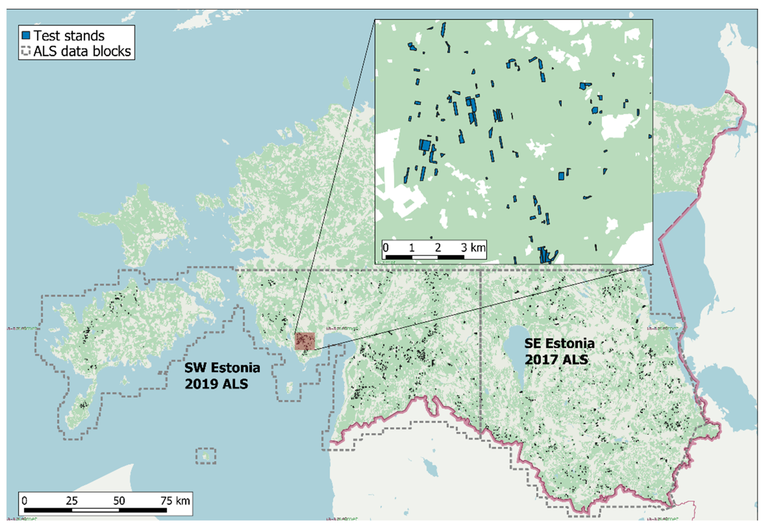
2.1. Forest Inventory and Management Data
2.2. Airborne Lidar Data
2.3. Random-Forest-Based Model Construction
2.4. General-Linear-Model-Based Prediction
3. Results
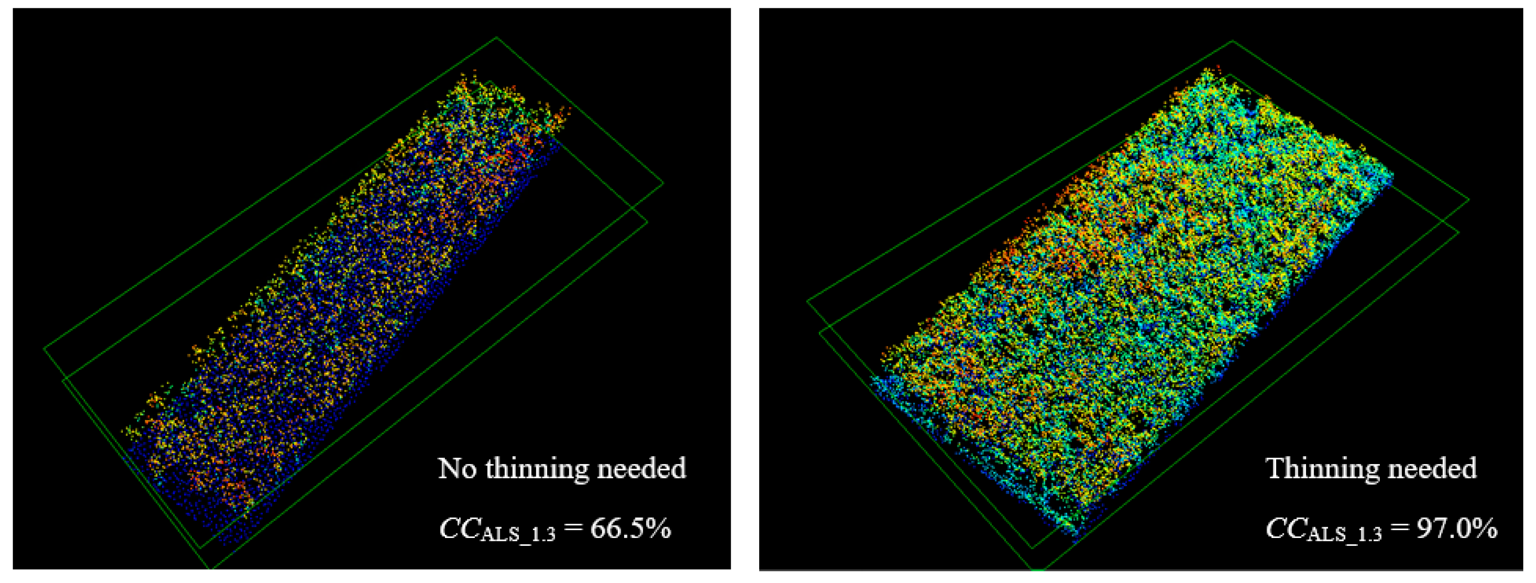
3.1. ALS Metrics
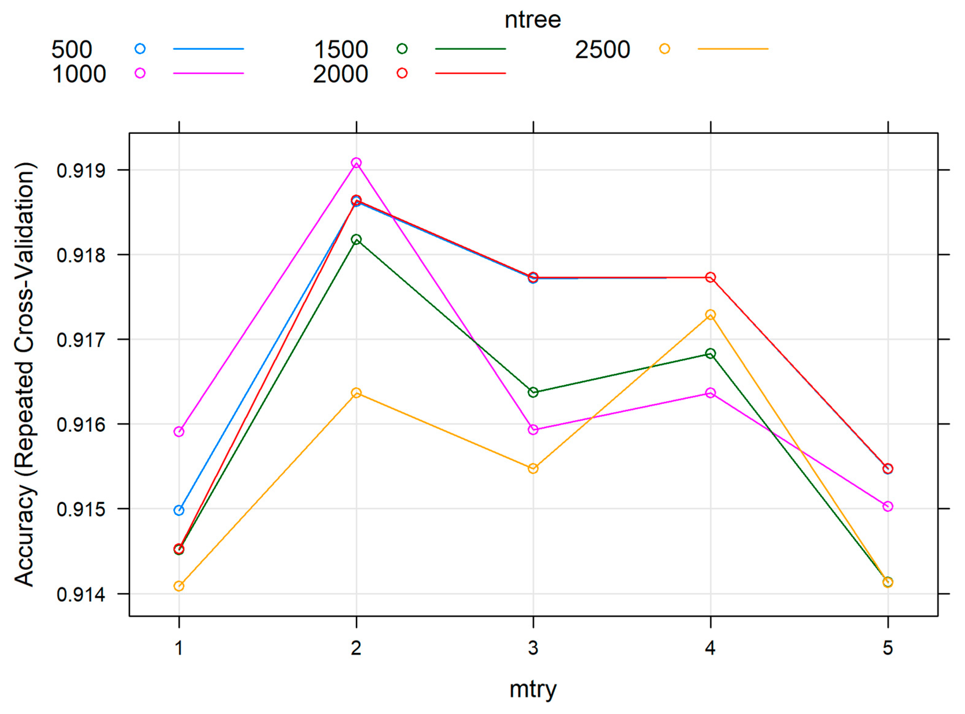
3.2. Random Forest Model Optimization
3.3. Validation and Decision Error Sensitivity Test
3.4. General-Linear-Model-Based Predictions
4. Discussion
5. Conclusions
Author Contributions
Funding
Acknowledgments
Conflicts of Interest
References
- Nelson, R.; Krabill, W.; MacLean, G. Determining forest canopy characteristics using airborne laser data. Remote Sens. Environ. 1984, 15, 201–212. [Google Scholar] [CrossRef]
- Tiner, R.W. Use of high-altitude aerial photography for inventorying forested wetlands in the United States. For. Ecol. Manag. 1990, 33-34, 593–604. [Google Scholar] [CrossRef]
- Lang, M.; Arumäe, T.; Anniste, J. Estimation of main forest inventory variables from spectral and airborne lidar data in Aegviidu test site, Estonia. For. Stud. 2012, 56, 27–41. [Google Scholar] [CrossRef]
- Arumäe, T.; Lang, M. ALS-based wood volume models of forest stands and comparison with forest inventory data. For. Stud. 2016, 64, 5–16. [Google Scholar] [CrossRef]
- Olesk, A.; Praks, J.; Antropov, O.; Zalite, K.; Arumäe, T.; Voormansik, K. Interferometric SAR Coherence Models for Characterization of Hemiboreal Forests Using TanDEM-X Data. Remote Sens. 2016, 8, 700. [Google Scholar] [CrossRef]
- Lang, M.; Kaha, M.; Laarmann, D.; Sims, A. Construction of tree species composition map of Estonia using multispectral satellite images, soil map and a random forest algorithm. For. Stud. 2018, 68, 5–24. [Google Scholar] [CrossRef][Green Version]
- Arumäe, T.; Lang, M. Estimation of canopy cover in dense mixed-species forests using airborne lidar data. Eur. J. Remote Sens. 2018, 51, 132–141. [Google Scholar] [CrossRef]
- Guerra-Hernández, J.; Arellano-Pérez, S.; González-Ferreiro, E.; Pascual, A.; Altelarrea, V.S.; Ruiz-González, A.D.; Álvarez-González, J.G. Developing a site index model for P. Pinaster stands in NW Spain by combining bi-temporal ALS data and environmental data. For. Ecol. Manag. 2021, 481, 118690. [Google Scholar] [CrossRef]
- Large, A.R.G.; Heritage, G.L. Laser Scanning for the Environmental Sciences. In Laser Scanning—Evolution of the Discipline; Heritage, G.L., Large, A.R.G., Eds.; John Wiley & Sons, Ltd.: West Sussex, UK, 2009; pp. 1–20. [Google Scholar]
- Zhao, Q.; Yu, S.; Zhao, F.; Tian, L.; Zhao, Z. Comparison of machine learning algorithms for forest parameter estimations and application for forest quality assessments. For. Ecol. Manag. 2019, 434, 224–234. [Google Scholar] [CrossRef]
- Hawryło, P.; Francini, S.; Chirici, G.; Giannetti, F.; Parkitna, K.; Krok, G.; Mitelsztedt, K.; Lisańczuk, M.; Stereńczak, K.; Ciesielski, M.; et al. The Use of Remotely Sensed Data and Polish NFI Plots for Prediction of Growing Stock Volume Using Different Predictive Methods. Remote Sens. 2020, 12, 3331. [Google Scholar] [CrossRef]
- McRoberts, R.E.; Tomppo, E.O. Remote sensing support for national forest inventories. Remote Sens. Environ. 2007, 110, 412–419. [Google Scholar] [CrossRef]
- Packalén, P.; Maltamo, M. The k-MSN method for the prediction of species-specific stand attributes using airborne laser scanning and aerial photographs. Remote Sens. Environ. 2007, 109, 328–341. [Google Scholar] [CrossRef]
- Ayrey, E.; Hayes, D.J. The Use of Three-Dimensional Convolutional Neural Networks to Interpret LiDAR for Forest Inventory. Remote Sens. 2018, 10, 649. [Google Scholar] [CrossRef]
- Breiman, L. Random forests. Mach. Learn. 2001, 45, 5–32. [Google Scholar] [CrossRef]
- Krigul, T. Metsatakseerimine; Valgus: Tallinn, Estonia, 1972. [Google Scholar]
- Rules of Forest Management. Available online: https://www.riigiteataja.ee/en/eli/ee/KKM/reg/521112017002/consolide (accessed on 22 November 2021).
- Zeide, B. Thinning and growth: A full turnaround. J. For. 2001, 99, 20–25. [Google Scholar] [CrossRef]
- Cameron, A.D. Importance of early selective thinning in the development of long-term stand stability and improved log quality: A review. Forestry 2002, 75, 25–35. [Google Scholar] [CrossRef]
- Bose, A.K.; Weiskittel, A.; Kuehne, C.; Wagner, R.G.; Turnblom, E.; Burkhart, H.E. Does commercial thinning improve stand-level growth of the three most commercially important softwood forest types in North America? For. Ecol. Manag. 2018, 409, 683–693. [Google Scholar] [CrossRef]
- Slodicak, M.; Novak, J. Silvicultural measures to increase the mechanical stability of pure secondary Norway spruce stands before conversion. For. Ecol. Manag. 2006, 224, 252–257. [Google Scholar] [CrossRef]
- Liu, Z.; Peng, C.; Work, T.; Candau, J.-N.; DesRochers, A.; Kneeshaw, D. Application of machine-learning methods in forest ecology: Recent progress and future challenges. Environ. Rev. 2018, 26, 339–350. [Google Scholar] [CrossRef]
- Lõhmus, E. Eesti Metsakasvukohatüübid; Eesti Loodusfoto: Tartu, Estonia, 2004. [Google Scholar]
- Orthophoto Metadata by Year. Available online: https://geoportaal.maaamet.ee/eng/Spatial-Data/Orthophotos/Orthophoto-metadata-by-year-p350.html (accessed on 22 November 2021).
- Dual Channel Waveform Processing Airborne Lidar Scanning System for High-Point Density and Ultra-Wide Area Mapping: Riegl VQ-1560i Datasheet. Available online: http://www.riegl.com/nc/products/airborne-scanning/produktdetail/product/scanner/55/ (accessed on 22 November 2021).
- McGaughey, R.J. FUSION/LDV: Software for LIDAR Data Analysis and Visualization. March 2014—FUSION; Version 4.00; United States Department of Agriculture Forest Service Pacific Northwest Research Station: Portland, OR, USA, 2020.
- R: A Language and Environment for Statistical Computing; R Foundation for Statistical Computing: Vienna, Austria; Available online: https://www.R-project.org/ (accessed on 22 November 2021).
- Strobl, C.; Boulesteix, A.-L.; Kneib, T.; Augustin, T.; Zeileis, A. Conditional variable importance for random forests. BMC Bioinform. 2008, 9, 307. [Google Scholar] [CrossRef]
- Louppe, G.; Wehenkel, L.; Sutera, A.; Geurts, P. Understanding variable importances in forests of randomized trees. In Advances in Neural Information Processing Systems; Burges, C.J.C., Bottou, L., Welling, M., Ghahramani, Z., Weinberger, K.Q., Eds.; Curran Associates Inc.: New York, NY, USA, 2013; pp. 431–439. [Google Scholar]
- Aastaraamat “Mets 2019”. Available online: https://keskkonnaagentuur.ee/media/882/download/ (accessed on 22 November 2021).
- Schumacher, J.; Hauglin, M.; Astrup, R.; Breidenbach, J. Mapping forest age using National Forest Inventory, airborne laser scanning, and Sentinel-2 data. For. Ecosyst. 2020, 7, 60. [Google Scholar] [CrossRef]
- Arumäe, T.; Lang, M. A simple model to estimate forest canopy base height from airborne lidar data. For. Stud. 2013, 58, 46–56. [Google Scholar] [CrossRef]


| Test Site | Thinning Necessity | Number of Stands | ALS Metrics | |
|---|---|---|---|---|
| Canopy Cover (%) | HP95 (m) | |||
| Southwestern Estonia | Yes | 637 | 85.1 (9.2) | 18.2 (3.6) |
| No | 416 | 71.9 (12.9) | 20.1 (5.7) | |
| Southeastern Estonia | Yes | 360 | 89.1 (7.8) | 20.5 (3.5) |
| No | 591 | 71.1 (27.1) | 25.4 (6.3) | |
| Test Site | ALS Metrics | Mean Decrease in Accuracy | Mean Decrease in Gini |
|---|---|---|---|
| Southwestern Estonia | Canopy cover | 138.4 | 115.8 |
| 95th height percentile | 56.1 | 65.4 | |
| Height MAD mode | 42.6 | 29.1 | |
| Coefficient of height variation | 23.3 | 17.6 | |
| 25th height percentile | 19.6 | 15.6 | |
| Southeastern Estonia | Canopy cover | 99.5 | 109.5 |
| 95th height percentile | 79.8 | 111.4 | |
| Height MAD mode | 36.8 | 34.3 | |
| Height skewness | 26.4 | 30.3 | |
| 20th height percentile | 20.9 | 29.1 |
| Test Area | Model Accuracy | ALS Metric | Parameter Value |
|---|---|---|---|
| Southwestern Estonia | 92.1% | 50th height percentile | −0.04817 (0.004) |
| Coefficient of height variation | −0.00209 (0.001) | ||
| Canopy cover above mean height Intercept | 0.02321 (0.001) | ||
| −0.28000 (0.045) | |||
| Southeastern Estonia | 81.8% | Mean height | −0.04887 (0.004) |
| Kurtosis of height | 0.06119 (0.011) | ||
| Canopy cover above mean height Intercept | 0.01193 (0.001) | ||
| 0.31203 (0.088) |
Publisher’s Note: MDPI stays neutral with regard to jurisdictional claims in published maps and institutional affiliations. |
© 2022 by the authors. Licensee MDPI, Basel, Switzerland. This article is an open access article distributed under the terms and conditions of the Creative Commons Attribution (CC BY) license (https://creativecommons.org/licenses/by/4.0/).
Share and Cite
Arumäe, T.; Lang, M.; Sims, A.; Laarmann, D. Planning of Commercial Thinnings Using Machine Learning and Airborne Lidar Data. Forests 2022, 13, 206. https://doi.org/10.3390/f13020206
Arumäe T, Lang M, Sims A, Laarmann D. Planning of Commercial Thinnings Using Machine Learning and Airborne Lidar Data. Forests. 2022; 13(2):206. https://doi.org/10.3390/f13020206
Chicago/Turabian StyleArumäe, Tauri, Mait Lang, Allan Sims, and Diana Laarmann. 2022. "Planning of Commercial Thinnings Using Machine Learning and Airborne Lidar Data" Forests 13, no. 2: 206. https://doi.org/10.3390/f13020206
APA StyleArumäe, T., Lang, M., Sims, A., & Laarmann, D. (2022). Planning of Commercial Thinnings Using Machine Learning and Airborne Lidar Data. Forests, 13(2), 206. https://doi.org/10.3390/f13020206