Evaluating the Performance of a Forest Succession Model to Predict the Long-Term Dynamics of Tree Species in Mixed Boreal Forests Using Historical Data in Northern Ontario, Canada

Abstract

Environmental concerns and economic pressures on forest ecosystems have led to the development of sustainable forest management practices. As a consequence, forest managers must evaluate the long-term effects of their management decisions on potential forest successional pathways. As changes in forest ecosystems occur very slowly, simulation models are logical and efficient tools to predict the patterns of forest growth and succession. However, as models are an imperfect representation of reality, it is desirable to evaluate them with historical long-term forest data. Using remeasured tree and stand data from three data sets from two ecoregions in northern Ontario, the succession gap model ZELIG-CFS was evaluated for mixed boreal forests composed of black spruce (Picea mariana [Mill.] B.S.P.), balsam fir (Abies balsamea [L.] Mill.), jack pine (Pinus banksiana L.), white spruce (Picea glauca [Moench] Voss), trembling aspen (Populus tremuloides Michx.), white birch (Betula papyrifera Marsh.), northern white cedar (Thuja occidentalis L.), American larch (Larix laricina [Du Roi] K. Koch), and balsam poplar (Populus balsamefera L.). The comparison of observed and predicted basal areas and stand densities indicated that ZELIG-CFS predicted the dynamics of most species consistently for periods varying between 5 and 57 simulation years. The patterns of forest succession observed in this study support gap phase dynamics at the plot scale and shade-tolerance complementarity hypotheses at the regional scale.

1. Introduction

Emulating natural disturbances in managed forests has been recommended as a means to sustainably manage boreal forests for timber production, climate regulation and climate change mitigation [1], biodiversity [2], and many other ecosystem services that are essential to human well-being [3,4,5]. These multiple social and environmental demands have led to increasing pressure on forest ecosystems. Consequently, forest managers must be concerned with the application of the basic principles of ecosystem management and integrity, which requires the evaluation and prediction of potential successional pathways [6,7]. Here, succession is defined as the directional change through time of species composition and vegetation physiognomy of a single site where climate remains relatively constant [8]. Bazzaz [9] introduced the notion of scale into the discussion of succession. In boreal forests, evidence points to gap dynamics at the local scale and species succession at the landscape scale.

For boreal forests, a growing body of evidence [10,11,12,13,14,15] suggests that emulating natural disturbances in managed forests should be performed in the context of forest gap dynamics theory [16]. Forest gap dynamics is a process that occurs when one or a few canopy trees die standing, snap off, or are blown to the ground, creating small ‘gaps’ in the forest canopy that are then filled with other trees [17,18]. Studies on gap dynamics of boreal forests provide evidence suggesting that, in the absence of broad-scale stand replacing disturbances, boreal forests can remain in the old-growth stage for long periods [1,10,11,13,14,15].

At the regional scale in boreal forests, species pools, density dependence, site resources and intermediate disturbances have all proven to be key mechanisms in species dynamics and coexistence over time [19]. Other mechanisms including shade-tolerance complementarity and resource ratio hypothesis may also drive species dynamics and coexistence. Resource-poor soils favour species that tolerate limited resources, whereas rich soils permit invasion and promote mixtures.

As forest gap models have a mechanistic basis to represent the effects of ecological site characteristics, including light and climatic conditions and basic soil properties, they are well equipped to predict the growth and development of uneven-aged mixed forests with complex structures [20]. In JABOWA [21] gap type models, individual-tree growth is governed by species-specific ecological properties, including shade tolerance, climatic response and effects of basic soil properties. Moreover, as they include model components to predict regeneration establishment and mortality, they can be used to address questions on long-term successional pathways.

Forest gap models have been used mostly as research tools for studying tree population dynamics and examining long-term theoretical succession questions or hypotheses [7,22,23,24]. Less importance has been given to the evaluation of their performance with regional forest ecosystems. Some models were validated by comparing their predictions against pollen records or potential natural vegetation development [22,25], but these two methods are not based on comparisons with long-term forest records. Relatively little effort has been devoted to testing the performance of gap models using long-term historical forest records, despite the fact that this issue has been raised several times in recent years [25,26,27,28]. Comparing model predictions against long-term observations is essential to build confidence in models and guide silvicultural operations when improved knowledge of changes in species composition is needed to maintain biodiversity or evaluate the potential effects of global change [6,25,27,28,29].

The relatively small number of studies that evaluated, validated or tested gap models in boreal mixedwood forests of Canada may be attributable to the limited availability of historical forest records containing long-term inventory or experimental sites with repeated measurements [25,26,27]. Using historical repeated measurements to evaluate the performance of gap models has two advantages. First, they allow comparison of long-term predicted changes in productivity and species composition with field observations, which may contribute to improving models. Second, comparisons over repeated long-term measurements provide the opportunity to evaluate the performance of models for various simulation periods. This approach may be a safeguard against random unpredictable fluctuations caused by unforeseen disturbances. As a result, agreement between observations and predictions may be high for some simulation periods, but low for other periods. For the boreal forest, the performance of gap models with repeated measurements was evaluated in studies that used a variety of models, such as SORTIE-ND, FAREAST, FORSKA-2V, BOREALIS, ForClim, and SIBBORK [26,28,30,31,32,33,34,35,36]. These studies provided invaluable results for the evaluation of gap models, but they had some limitations. In some studies, data sets included many sample plot data, but comparisons between observations and predictions were performed at a single point in time. For other studies, comparisons between observations and predictions were conducted with long-term historical data, but only a few sample plot data were used or sample plot data contained only few species. As such, these justify the need for further research that can take advantage of historical remeasurement data sets. The objective of this study was to evaluate the extent to which the gap model ZELIG-CFS [37] realistically predicted the long-term dynamics of tree species in mixed boreal forest types in northern Ontario, Canada, using historical long-term observations.

2. Materials and Methods

2.1. Study Area

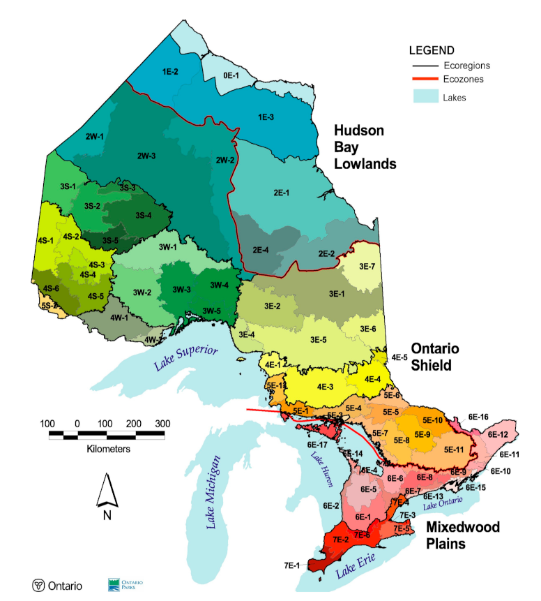
This study was conducted using historical data obtained from the boreal forest region of northern Ontario in ecoregions 3E and 3W in the middle section of the boreal forest of the Ontario Shield Ecozone (Figure 1). Details on ecological characteristics may be found in [38]. A brief summary follows. The area of this ecozone is approximately 65 millions hectares (ha) with variable topography and its climate is characterized by long, cold and moist winters and short warm summers. Variations in temperature and precipitations are considerable. In average, daily temperatures are approximately −15 and 17 °C in January and July, respectively. As the ecoregions 3E and 3W differ in basic ecological characteristics, results are presented separately. Ecoregion 3E is in the Humid Mid-Boreal ecoclimatic region. Precipitation varies between 652 and 1029 mm year⁻¹. Its deposits consist of morainal clays in the northeastern part, while ground moraine is generally found in most other areas. Soils consist mostly of podzols. The ecoclimatic region of ecoregion 3W is moist mid-boreal with lower annual precipitations than ecoregion 3E, varying from 654 to 879 mm. The geology of this ecoregion consists of granitic bedrock, but also includes basalt and volcanic rocks, greenstone, siltstone and shale. Soils consist of brunisols and podzols. The following tree species were found in both ecoregions: black spruce (Picea mariana [Mill.] B.S.P.), balsam fir (Abies balsamea [L.] Mill.), jack pine (Pinus banksiana L.), white spruce (Picea glauca [Moench] Voss), trembling aspen (Populus tremuloides Michx.), white birch (Betula papyrifera Marsh.) northern white cedar (Thuja occidentalis L.), American larch (Larix laricina [Du Roi] K. Koch) and balsam poplar (Populus balsamifera L.) (

Table 1. Average basal area (m² ha⁻¹) for tree species by ecoregion included in the study in northern Ontario, Canada.

Species	Ecoregion 3E	Ecoregion 3W
Black spruce	17.89 (0.005, 46.61) 1	14.23 (0.007, 49.05)
Balsam fir	2.53 (0.001, 22.19)	2.01 (0.006, 20.25)
Jack pine	7.59 (0.016, 44.18)	17.49 (0.053, 47.23)
White spruce	1.79 (0.006, 5.91)	1.37 (0.004, 12.99)
Trembling aspen	20.31 (0.012, 45.38)	13.85 (0.028, 65.70)
White birch	2.30 (0.002, 19.82)	3.43 (0.009, 15.70)
Northern white cedar	0.72 (0.008, 8.25)	0.95 (0.58, 2.17)
American larch	3.22 (0.133, 9.14)	1.08 (0.072, 5.46)
Balsam poplar	7.22 (0.005, 34.37)	2.92 (0.006, 18.19)

¹ Minimum and maximum values in parentheses.

). The importance of species composition differed between ecoregions 3E and 3W. Mean basal area was higher in Ecoregion 3E than 3W for black spruce, trembling aspen, American larch, and balsam poplar, but the opposite for jack pine and white birch. Differences in mean basal area between both ecoregions were relatively small for balsam fir, white spruce and northern white cedar. For the range of variation between minimum and maximum values, differences between the ecoregions were pronounced for white spruce, trembling aspen, white birch, northern white cedar, American larch and balsam poplar.

2.2. Historical Forest Data Sets

The individual-tree sample plot data used in this study to compare model predictions against observations were obtained from three data sets maintained by the Ontario Ministry of Northern Development, Mines, Natural Resources and Forestry (NDMNRF): American Can, Kimberly Clark and Spruce Falls Power and Paper Co. (SFPP), which included 148, 115 and 113 sample plots, respectively. Measurements were conducted between 1951 and 2000 for American Can, between 1952 and 2000 for Kimberly Clark and between 1930 and 1989 for SFPP. All the trees in each sample plot were measured for diameter at breast height (dbh). For all three data sets, the combination of sample plots and remeasurement periods resulted in tree measurements that exceeded 1 million records (

Table 2. Basic statistics (mean and range) of stand density and diameter at breast height (dbh) and number of tree measurements for data sets in the boreal forest of northern Ontario.

Species	Stand Density	Dbh (cm)	Number of Tree
	(Trees ha−1)		Measurements
American Can
Black spruce	1243 (12, 8961) 1	9.2 (0.8, 63.2)	84,258
Balsam fir	550 (12, 4697)	6.6 (0.3, 50.0)	31,963
Trembling aspen	563 (12, 5278)	16.3 (1.3, 71.7)	26,613
White birch	455 (12, 9546)	9.0 (0.3, 50.3)	20,826
Jack pine	675 (12, 7713)	14.5 (1.3, 53.8)	18,273
American larch	627 (12, 2841)	6.7 (1.3, 28.9)	3099
Northern white cedar	326 (12, 4299)	4.6 (1.3, 34.5)	2408
White spruce	102 (12, 1124)	8.9 (0.8, 54.0)	1448
Balsam poplar	206 (12, 1211)	12.7 (1.3, 42.0)	1321
Kimberly Clark
Black spruce	991 (12, 4573)	12.6 (1.3, 37.8)	50,600
Jack pine	728 (12, 6440)	16.8 (2.0, 46.5)	33,756
Trembling aspen	331 (12, 3164)	17.2 (2.0, 55.4)	8051
White birch	203 (12, 853)	10.9 (2.0, 37.8)	4947
Balsam fir	136 (12, 2546)	10.0 (1.5, 45.0)	2742
Balsam poplar	330 (12, 457)	17.8 (2.5, 39.4)	1246
White spruce	53 (12, 420)	19.2 (1.3, 61.5)	935
American larch	18 (12, 37)	10.3 (4.1, 14.5)	9
Spruce Falls Power and Paper Co.
Black spruce	2444 (2, 20,306)	8.5 (2.5, 55.9)	565,094
Balsam fir	650 (2, 12,592)	5.2 (2.5, 43.2)	108,563
Trembling aspen	217 (2, 8848)	11.9 (2.5, 63.5)	58,859
White birch	117 (2, 988)	9.7 (2.5, 53.3)	16,317
Balsam poplar	334 (2, 4744)	11.5 (2.5, 73.7)	40,555
Jack pine	225 (2, 2835)	15.2 (2.5, 48.3)	11,810
American larch	89 (2, 781)	8.7 (2.5, 38.1)	9274

¹ Minimum and maximum values in parentheses.

).

For all three data sets, stand age varied between 5 and 214 years. Most sample plots were remeasured every 5 years (

Table A1. Number of measurements for different time intervals between two measurements for the data sets used in this study.

Time Interval between Two Measurements	Number of Time Intervals between Two Measurements
(Year)	American Can	Kimberly Clark	Spruce Falls Power and Paper Co.
1		2	5
2	1	4	5
3	1	3	15
4	12	5	50
5	404	387	706
6		5	155
7		7	7
8		9	8
9		7	35
10	77	46	25
11	53	11	10
12		24	2
13	1	24
14		1	1
15		2	10
16		1	2
17			2
18	20		1
19		2
20		2
21	3	1	3
22	21		1
23		1
24		2
25			3
28	1	1
29			2
30		1
31			1
32	1
35			1
36			1
41	1		1
49			1

). Remeasurement intervals between 1 and 4 years and between 6 and 49 years were less frequent. The number of sample plots in different age classes varied substantially (

Table 3. Number of sample plots in different age classes and minimum and maximum duration of remeasurements. For each sample plot, age class consists of stand age at first measurement.

Age Class	Number of	Duration of Remeasurements (Year)
(Year)	sample plots	Minimum	Maximum
5 to 19	10	10	56
20 to 29	19	5	51
30 to 39	50	20	55
40 to 49	27	5	49
50 to 59	44	5	57
60 to 69	37	10	56
70 to 79	39	5	48
80 to 89	70	5	56
90 to 99	34	5	47
100 to 109	15	5	48
110 to 119	8	15	48
120 to 129	5	15	48
130 to 139	7	18	48
160 to 169	10	10	48
≥170	1	15	15

). Relatively high numbers of sample plots were found in the age classes from 30 to 39 to 90 to 99 years. The duration of remeasurements generally varied from a minimum of 5 years to a maximum of 56 years. Most of the maximums were close to 50 years. Sample plot size varied between 400 and 4047 m² (

Table A2. Plot size distribution for the sample plot data in the three data sets used in this study maintained by the Ontario Ministry of Natural Resources and Forestry.

Data Set	Plot Size (m2)	Number of Sample Plots
American Can	400	3
	404.7	4
	506	17
	809	124
Kimberly Clark	809	115
Spruce Falls Power and Paper Co.	404	10
	405	1
	1011	24
	1012	3
	1214	1
	2023	32
	2043	1
	2428	1
	3035	1
	4046	9
	4047	31

). The majority of them measured 809 m² in size (30.5%). While the sample plots for the American Can data set were in ecoregions 3E and 3W, the sample plots for Kimberly Clark and SFPP were in 3W and 3E, respectively (

Table 4. Number of sample plots for each data set by ecoregions included in the study in northern Ontario, Canada.

Data Set	Ecoregion 3E	Ecoregion 3W
American Can	68	80
Kimberly Clark		115
Spruce Falls Power and Paper Co.	113

). The sample plots were established on sites of natural origin and soils that had sandy, sandy-loam, loam, silty-loam or clayey-loam textures. However, for the SFPP data set, 21 sample plots originated from stands that were cut or cut and burned.

Variation in stand density and dbh was considerable for most species (Table 2). For stand density, substantial variations were evident for black spruce, balsam fir, trembling aspen, jack pine and white birch in the three data sets, but were less pronounced for the other species. Low species density values observed may be related to the mixed nature of the stands. Only 2.3% of the stands contained 1 species, which consisted of black spruce, but 68.2% of the stands included between 4 and 6 species. Approximately one-quarter of the stands were composed of 2 or 3 species (22%) and 7.4% had 7 or 8 species. Thus, variations in species proportions were important among the stands, varying from small to large presence.

2.3. Overview of ZELIG-CFS

ZELIG-CFS, a gap model that belongs to the JABOWA [21] type model, simulates individual-tree growth and mortality and regeneration on an annual time step. Its core structure is based on the integration of species-specific ecological properties (

Table 5. Ecological trait database used in the ZELIG-CFS model to simulate forest stand conditions for mixed species forests in northern Ontario, Canada.

Species	Mage 1	Dmax	Hmax	DDmin	DDmax	Toler	Drought	Nutri
Black spruce	250	40	2000	265	1929	2	3	3
Balsam fir	200	65	3000	250	2404	1	1	3
Jack pine	150	50	2500	213	2234	5	4	3
White spruce	200	64	3000	447	1929	2	3	3
Trembling aspen	125	75	3700	889	5556	5	3	2
White birch	250	150	4500	1420	3084	3	2	2
Northern white
cedar	400	100	2900	1000	2188	2	4	3
American larch	335	75	2500	280	2660	5	4	3
Balsam poplar	150	75	2500	555	2491	5	1	3

¹ Mage is the maximum expected age for a species (year), Dmax is maximum diameter at breast height (cm) that a species can reach in its area of distribution, Hmax is the maximum height (cm) that a species can reach in its area of distribution, DDmin and DDmax are the minimum and maximum growing degree-days needed for a species to grow, Toler is species-specific shade tolerance class (1 = shade tolerant; 5 = shade intolerant), Drought is the species-specific drought tolerance class (1 = very drought-intolerant; 5 = very drought tolerant), and Nutri represents a soil fertility response class (1 = nutrient stress intolerant; 3 = nutrient stress tolerant).

) and representation of local environmental growth conditions, including monthly mean temperatures and precipitations, site fertility, and light interception at the individual-crown and canopy scales at different height strata on tree growth and seedling establishment. The basic approach in modelling tree growth consists in computing species-specific potential diameter increment (calculated from Dmax in Table 5), which is then modified by light available growing factor and species-specific shade tolerance class (Toler in Table 5), site growing degree-days parabolic response functions (estimated from temperature values and DDmin and DDmax in Table 5), soil moisture (estimated from precipitation values), and a soil fertility factor (estimated from site-specific potential biomass production). Regeneration establishment is modelled based on potential number of seedlings that can germinate on a site modified by understory light conditions adjusted by species-specific shade tolerance class, growing degree-days and soil moisture and fertility response classes.

ZELIG-CFS originates from the ZELIG model [39,40,41], but was modified to improve the representation of some processes. The major modification was made to the modelling of the available light growing factor (ALGF) and its effect on species-specific dbh growth rate. In ZELIG, individual-tree leaf area is assumed to be distributed uniformly with crown depth. In ZELIG-CFS, a sigmoidal cumulative leaf area distribution function is computed to more realistically represent the pattern of changes in light conditions with crown depth that integrates species-specific shade tolerance classes, which influences how crown recession rate occurs and, ultimately, dbh growth rate. Additionally, as crown recession takes place, change in crown width is adjusted based on species-specific crown shape functions: (1) a parabolic function for white spruce, northern white cedar, trembling aspen, jack pine and balsam poplar, (2) an ellipsoid function for American larch and white birch, (3) a conical function for balsam fir and (4) a cylindrical function for black spruce. This approach is consistent with findings reported by [42,43,44,45]. Other modifications were made to the mortality and regeneration model components. Mortality is handled by computing species-specific survival probability functions from dbh and dbh growth rate. For regeneration, a stocking factor representing space occupancy was added to the model. ZELIG-CFS was used to successfully predict the development of North American mixed forest types, including hardwood and softwood species [37,46] and subtropical dry forests [47].

2.4. Initialization Files

The development of each sample plot of the three data sets was simulated. For each sample plot, basic site information, including plot area and shape, latitude, longitude, altitude, soil field capacity and wilting points, soil fertility factor and monthly mean temperature and precipitation along with their standard deviations were stored in initialization files. Standard deviations for climatic data are used to randomly select monthly mean temperature and precipitation variations over the course of simulations. Site-specific monthly mean temperature and precipitation values were obtained from BIOSIM, an application that is used interpolate temperature and precipitation among regional weather stations [48].

Individual-tree data provided for each sample plot in the initialization files included tree number, species code and dbh. The first tree dbh measurements for each sample plot of the data sets were used as initialization data to initiate the simulations. They were considered as the state of the stands at simulated year 0. For each plot, the periodic observed data obtained from remeasurements over time were relative to simulated year 0, which facilitated the matching of observed and predicted basal areas and stand densities at specific simulated years.

Initial regeneration data provided as input in the initialization files included number of seedlings per square meter and stocking. The number of seedlings is, in fact, a potential number of seedlings per species that may germinate every year during the simulations. This number is then adjusted in every simulation year by a random value that represents the natural variability, understory light conditions, soil moisture and fertility and air temperature [37]. Stocking represents the proportion of the area that seedlings of a species may occupy within a forest ecosystem.

As regeneration data were not available in the data set, a procedure was developed to derive realistic estimates for both potential number of seedlings and stocking by assuming that regeneration was related to species-specific density in the tree layer at the individual-plot scale. A literature review on regeneration studies conducted in the boreal forest of northern Ontario and Quebec allowed us to identify several studies providing results on both seedling abundance and stocking [49,50,51,52,53,54,55,56,57]. As no regeneration study was found for northern white cedar in northern Ontario or Quebec, values documented by [58] in the Ottawa valley, near the southern limit of the boreal forest were used.

For each sample plot and species within each data set, the potential number of seedlings (PNS) provided in the initialization files to run the simulations was estimated as:

$$\mathrm{PNS} = \mathrm{MNS}\times \mathrm{STD}/\mathrm{MAD}$$

(1)

where MNS is an estimate of the maximum number of seedlings per m² that can be found in northern Ontario, as determined from the literature, STD the species-specific tree density in a sample plot and MAD the maximum species-specific tree density observed in the data set.

For each species present in the sample plots, stocking values (STOCK) were estimated as:

$$\mathrm{STOCK}=\mathrm{MINS}+\left(\mathrm{STD} - \mathrm{MIND}\right) \times \left(\mathrm{MAXS} - \mathrm{MINS}\right)/\left(\mathrm{MAD} - \mathrm{MIND}\right)$$

(2)

where MINS is the minimum stocking value that can be found in northern Ontario, MIND the minimum species-specific tree density observed in the data set, and MAXS the maximum stocking value determined from the literature.

For the initialization files, balsam fir had the highest estimated average potential number of seedlings per m², followed by trembling aspen, black spruce and northern white cedar (

Table 6. Average potential number of seedlings per m² and stocking values for each species provided as input for the sample plots in the initialization files.

Species	Number of Seedlings m−2	Stocking (Proportion)
Black spruce	0.4552 (0.5135) 1	0.262 (0.191) 1
Balsam fir	5.7385 (65.8297)	0.278 (0.253)
Jack pine	0.0096 (0.0195)	0.119 (0.123)
White birch	0.0534 (0.1246)	0.314 (0.304)
White spruce	0.0045 (0.0230)	0.010 (0.026)
Balsam poplar	0.0027 (0.0226)	0.057 (0.116)
Trembling aspen	0.7808 (2.3265)	0.119 (0.151)
Northern white cedar	0.1421 (0.2519)	0.145 (0.039)
American larch	0.0069 (0.0254)	0.079 (0.164)

¹ Standard deviation.

). The potential numbers of seedlings were much lower for jack pine, white spruce, white birch, American larch and balsam poplar. The large numbers of seedlings per m² for balsam fir and black spruce were also associated with relatively high average stockings (Table 6). The highest average stocking was observed for white birch, but was not associated with a relatively high potential number of seedlings. Trembling aspen was among the species with high potential number of seedlings, but had a relatively low stocking. Relatively lower stocking values were observed for jack pine, white spruce, northern white cedar, American larch and balsam poplar. Relatively large standard deviations indicated much variation in the potential number of seedlings and stocking among the sample plots for each species. As the presence of northern white cedar was very marginal, simulation results for this species were not included here.

2.5. Data Analysis

Three statistics were computed to compare model predictions against observed plot attributes, including basal area and stand density over time. Both basal area and stand density were computed for each plot and by species and year and then averaged for each year. The relative model bias was computed to compare predicted and observed basal areas for each sample plot as:

$$\mathrm{Bias}=\lfloor \frac{\mathrm{Predictions} - \mathrm{observations}}{\mathrm{observations}}\times 100\rfloor$$

(3)

This statistic was discussed in several studies that evaluated the performance of models [23,27,59,60]. It was averaged among plots to calculate an agreement indicator between simulated and observation data. High agreement between simulations and observations is associated with a low bias value. Negative values indicate that a model underestimates, while positive values indicate that it overestimates.

Model efficiency (ME) was computed to evaluate the capacity of a model to reproduce observations on a relative scale with values below 0 indicating a poor performance and 1 perfect performance [59]. It is computed as:

$$\mathrm{ME} = 1 - \frac{{{\displaystyle \sum }}^{ }{\left({\mathrm{y}}_{\mathrm{i}}-{\hat{\mathrm{y}}}_i\right)}^2}{{{\displaystyle \sum }}^{ }{\left({\mathrm{y}}_{\mathrm{i}}-\overline{\mathrm{y}}\right)}^2}$$

(4)

where ${\mathrm{y}}_{\mathrm{i}}$ is observation i, ${\hat{\mathrm{y}}}_i$ prediction i, and $\overline{\mathrm{y}}$ the average of observations.

Observed and predicted diameter distributions were compared by computing a similarity coefficient (PS) [25] for every observation year to evaluate the extent to which observed and predicted dbh distributions differed:

$$\mathrm{PS}=1 - \frac{{{\displaystyle \sum }}_{\mathrm{i}=1}^{\mathrm{n}}{|\mathrm{x}}_{\mathrm{i}}{- \mathrm{y}}_{\mathrm{i}}|}{{{\displaystyle \sum }}_{\mathrm{i}=1}^{\mathrm{n}}\left({\mathrm{x}}_{\mathrm{i}}{+\mathrm{y}}_{\mathrm{i}}\right)}$$

(5)

where x_i and y_i are the predicted and observed numbers of trees in dbh class i, respectively. This coefficient varies between 0 and 1 and indicates the proportion of values common to predicted and observed data sets [61].

3. Results

3.1. Basal Area

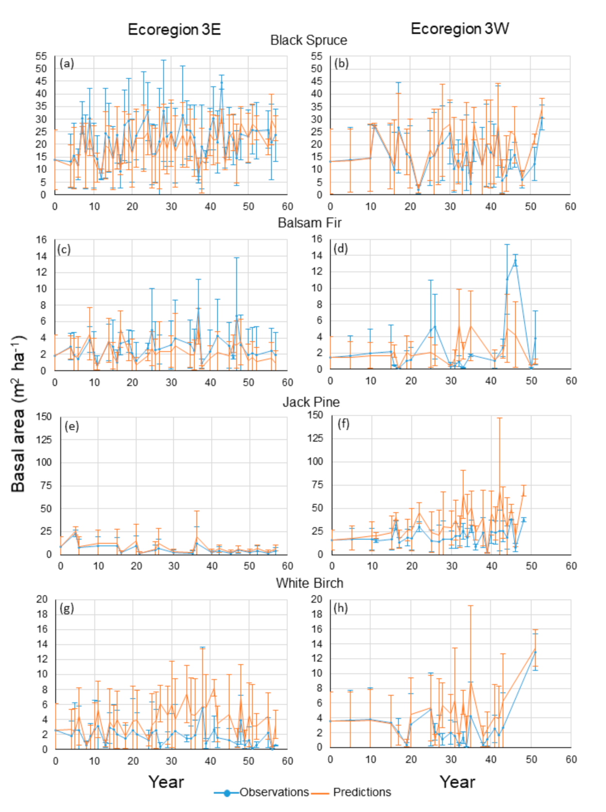
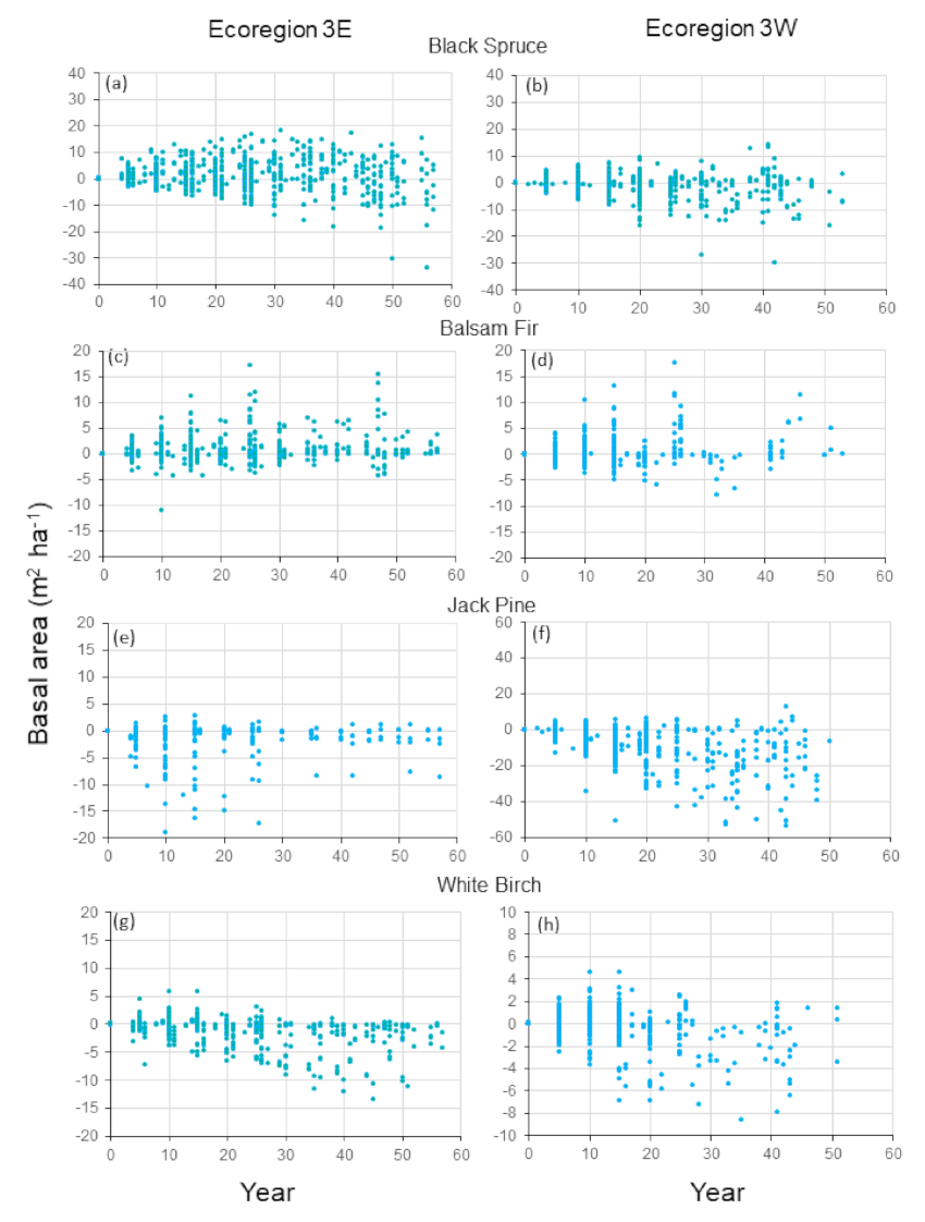
Agreement between mean predicted and observed basal areas was high for black spruce in the two ecoregions for nearly every year and the standard deviations between observations and predictions overlapped considerably (Figure 2a,b). For Ecoregion 3E, percentages of differences between observations and predictions smaller than 2 and 5 m² ha⁻¹ in absolute values were 54 and 78%, respectively (Figure 3a). The maximum amplitudes of the majority of the differences were ±10 m² ha⁻¹ over years and the number of differences smaller or higher than −10 or 10 m² ha⁻¹ were marginal, representing only 6% of the differences. The same statistics for differences smaller than 2 and 5 m² ha⁻¹ in absolute values for Ecoregion 3W were 73 and 90%, with a pronounced proportion of negative differences (Figure 3b). Only 2.9% of the differences between observations predictions were smaller or higher than 10 m² ha⁻¹ over years and were observed in the past 30 years. Fluctuations were important for both ecoregions, but most of them occurred in the same years for predictions and observations (Figure 3a,b). Mean basal area increased slightly over time in Ecoregion 3E. For Ecoregion 3W, there was a relatively stable pattern of change over time, despite fluctuations.

The pattern of change over years in mean basal area for balsam fir was relatively stable for both ecoregions, but fluctuations were more pronounced than those for black spruce and did not always occur in the same years, particularly in Ecoregion 3W (Figure 2c,d). For Ecoregion 3W, agreement between predictions and observations was reasonably high from years 0 to 15, and for years 19, 20, 30, 41, 41 and 50, with large overlaps between the standard deviations of observations and predictions. At the plot scale and by year, 82 and 94% of the differences between predictions and observations in Ecoregion 3W were less than 2 and 5 m² ha⁻¹, respectively, and were within the same amplitude of differences over years (Figure 3d). Only 6% of the differences between observations and predictions were higher than 5 m² ha⁻¹. A close examination of the sample plot data in observation years 25 and 26 indicated that the large differences between observations and predictions were caused by extreme values in nine sample plots. The pronounced increases in basal area that was observed from years 25 to 26 and from years 44 to 46, which increased the differences between observations and predictions, were probably caused by measurement or record errors in the historical data. Differences between mean predictions and observations for Ecoregion 3E were generally less pronounced than in Ecoregion 3W, but comparable percentages of differences among sample plots and years were observed: 83 and 95% were less than 2 and 5 m² ha⁻¹ in absolute values, respectively (Figure 3c). The range of variation was the same over years, except for some large differences at years 10, 25, 26 and 47, which represented 2.5% of the total number of differences. Substantial overlaps in the standard deviations of observations and predictions and the occurrences of fluctuations were evident at the same time for most years.

Agreement between mean observations and predictions was high for jack pine in Ecoregion 3E, which was characterized by a slight pattern of decrease over time (Figure 2e). Differences between predictions and observations smaller than 2 and 5 m² ha⁻¹ represented 77 and 87% of the differences at the plot scale and by year. The amplitude of variation was relatively homogeneous over years, except for some large negative differences from year 10 to 60 (Figure 3e), representing 13% of the total number of differences. For Ecoregion 3W, mean observed and predicted basal areas for jack pine more than doubled in 48 years, despite fluctuations (Figure 2f). Differences between mean predictions and observations were generally higher than those in Ecoregion 3E (Figure 3f), but their standard deviations overlapped considerably for most years: 50 and 63% of the differences between observations and predictions were less than 2 and 5 m² ha⁻¹ in absolute values, respectively, over years.

Mean predicted and observed basal areas for white birch in Ecoregion 3E fluctuated considerably and generally did not occur the same years (Figure 2g). Agreement was high between mean observations and predictions for the first 25 years. Then, differences generally increased until year 50, but were all not pronounced: 80 and 91% of the differences between observations and predictions were smaller than 2 and 5 m² ha⁻¹ in absolute values, respectively (Figure 3g). The greatest differences between observations and predictions were observed from years 27 to 51 (8%). Mean observed and predicted basal areas in Ecoregion 3W were characterized by a pattern of decrease in the first 40 years, followed by a sharp increase (Figure 2h). Agreement was high between predictions and observations for the first 15 years. Then, relatively large negative differences were observed between years 15 and 43, with no strong overlap between the standard deviations of predictions and observations. When considered at the plot scale and by year, these relatively large differences can be attributed to sharp decreases in observations for some years only (Figure 3h), considerably decreasing the mean values. Despite these discrepancies, 86 and 96% of the differences between predicted and observed basal areas were less than 2 and 5 m² ha⁻¹ over years, respectively.

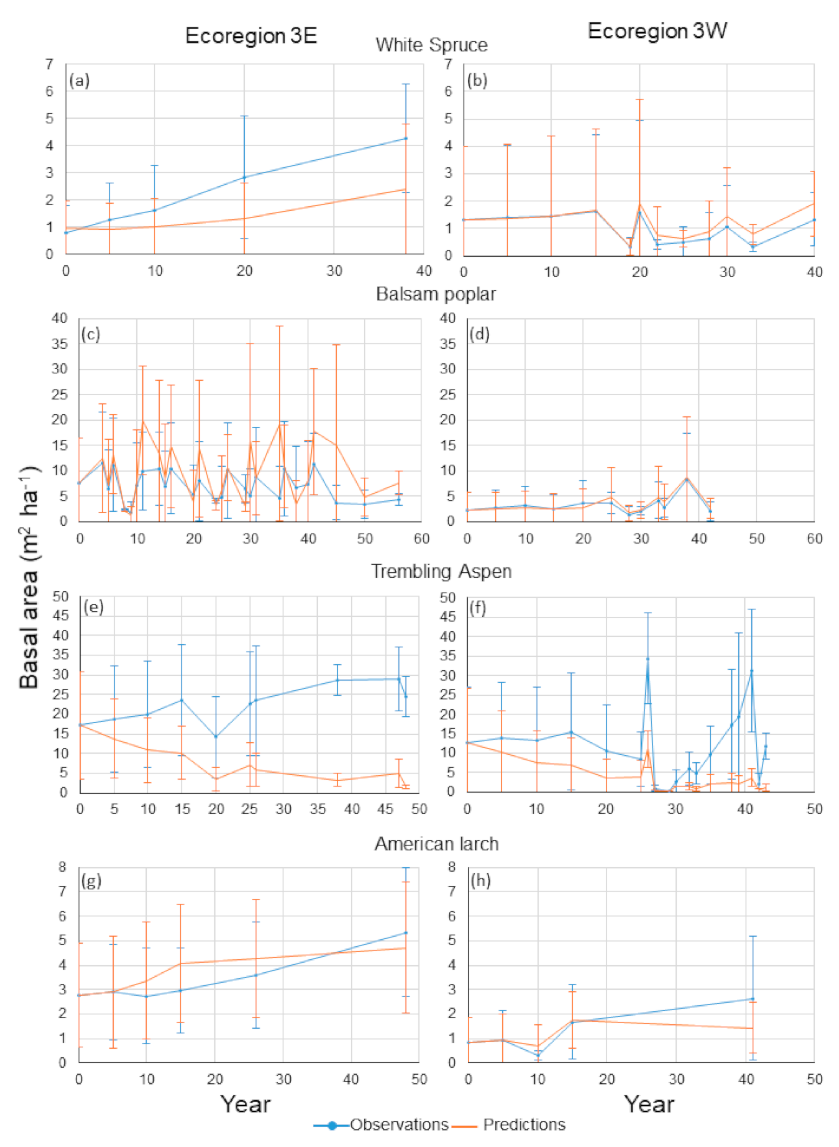
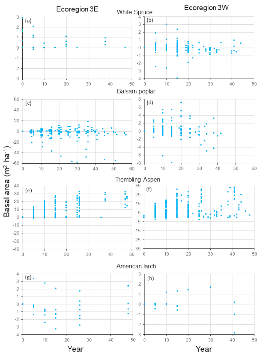
Compared to the other species, white spruce occupied small proportions of the stands, as indicated by the relatively small basal area values (Figure 4a,b). Mean predictions and observations were similar until year 10 and their standard deviations overlapped considerably for Ecoregion 3E (Figure 4a). However, compared to other species, there was a higher agreement between observations and predictions: 72% of the differences between predictions and observationsover years were smaller than 1 m² ha⁻¹ and only 2 differences were greater than 2 m² ha⁻¹ (Figure 5a). Even though differences between mean predictions and observations increased over years (Figure 4a), they remained relatively small (Figure 5a). Agreement was high between mean predicted and observed basal areas in Ecoregion 3W for all years (Figure 4b). The standard deviations for both mean predictions and observations overlapped considerably and fluctuations occurred in the same years. Deviations between observations and predictions were similar to those in Ecoregion 3E: 95% of the differences between predictions and observations were smaller than 1 m² ha⁻¹ in absolute values (Figure 5b).

Mean predictions and observations for balsam poplar in Ecoregion 3E fluctuated, with no obvious pattern of increase or decrease over time (Figure 4c). Despite apparent large discrepancies, the percentages of differences smaller than 2 and 5 m² ha⁻¹ between predictions and observations were 62 and 81%, respectively, over years (Figure 5c). Very large differences between mean predictions and observations at years 11, 21, 30, 35 and 45 also resulted from sudden decreases in observed basal area relative to previous years in some sample plots. However, the number of large differences between observations and predictions represented only 12% of these values. Mean predictions and observations for balsam poplar in Ecoregion 3W were very close and their standard deviations overlapped considerably (Figure 4d) and 76% of the differences between predictions and observations over years were less than 1 m² ha⁻¹ (Figure 5d).

Results for trembling aspen were not as consistent as those for the other species. Large differences between mean predictions and observations were observed for nearly every year in Ecoregion 3E and standard deviations did not much overlap (Figure 4e). Large positive differences between predictions and observations were observed nearly every year (Figure 5e). For Ecoregion 3W, mean predicted basal area decreased over years and mean observed basal area fluctuated considerably (Figure 4f). However, agreement was relatively high for years 29, 30 and 42. In years 5, 10, 15, 25 and 32, the standard deviations for both predictions and observations overlapped. Despite large differences between mean predictions and observations for several years, 52 and 66% of the differences between observations and predictions were less than 2 and 5 m² ha⁻¹, respectively (Figure 5f). The large differences for years 26, 35 to 41 and 43 were caused by high mortality rates predicted by ZELIG-CFS for some sample plots.

American larch occupied a small proportion of the forests compared to the other species (Figure 4g,h). For the two ecoregions, agreement was high between mean predictions and observations and their standard deviations largely overlapped. Over years, 57 and 81% of the differences between observations and predictions were less than 1 m² ha⁻¹ for ecoregions 3E and #w, respectively (Figure 5g,h).

Bias values indicated that, on average, ZELIG-CFS slightly underestimated basal area for black spruce in ecoregions 3E and 3W, but slightly overestimated basal area for jack pine in Ecoregion 3E (

Table 7. Average bias and model efficiency coefficients between observations and predictions by Ecoregion included in the study in northern Ontario, Canada.

	Ecoregion 3E		Ecoregion 3W
		Model	Model
Species	Bias (%)	efficiency	Bias (%)	efficiency
Black spruce	−3.3	0.85	−0.82	0.93
Balsam fir	96.39	0.47	0.88	0.4
Jack pine	0.47	0.45	27.35	−0.22
White birch	132.78	0.38	51.63	0.78
White spruce	−18.74	0.74	23.07	0.94
Balsam poplar	252.41	0.55	−0.02	0.7
Trembling aspen	−34	0.04	−29.96	0.54
American larch	26.71	0.57	12.21	0.66

). In Ecoregion 3E, high positive bias values were observed for balsam fir, white birch, balsam poplar and American larch, but relatively high negative bias for white spruce and trembling aspen. Balsam fir and balsam poplar had high average bias values in Ecoregion 3E, but lower average bias values in Ecoregion 3W. The reverse was observed for jack pine between Ecoregions. In absolute values, lower bias values were observed for white birch, trembling aspen and American larch in Ecoregion 3W than in 3E. While a negative bias was observed for white spruce in Ecoregion 3E, a positive bias was observed in Ecoregion 3W. In many cases, high bias values were caused by extremes that were not necessarily associated with many substantial differences between predictions and observations. For instance, 25% of the bias values at the combined plot scale and by year for balsam fir in Ecoregion 3E were less than 10% and most of the high bias values occurred in simulation results past 20 years. Additionally, high bias values were observed in many sample plots that did not contain many trees of particular species. For instance, predicted basal area for balsam fir in a sample plot was 0.011 m² ha⁻¹, but observed basal area was 0.056 m² ha⁻¹, which resulted in a bias of 80% in absolute value. The predicted basal area represented 15 small trees with average dbh of 2.5 cm over 184 trees in a 809 m² sample plot. For the other five species in the sample plot, average dbh was 9 cm, with 42 trees larger than 15 cm in dbh. This pattern was observed in several sample plots for species with high average bias values (data now shown).

Model efficiency was fairly high for black spruce and white spruce in both ecoregions and for white birch and balsam poplar in Ecoregion 3W (Table 7). It was greater than 0.50 for American larch in both ecoregions, and trembling aspen in Ecoregion 3W, between 0.40 and 0.50 for balsam fir in both ecoregions and jack pine in Ecoregion 3E, and very low for trembling aspen in Ecoregion 3E. Only two negative values were observed: balsam poplar in Ecoregion 3E and jack pine in Ecoregion 3W. Low or negative values of model efficiency observed for some species can be associated with the occurrence of substantial differences between observations and predictions, but they did not affect the general patterns of similarity of changes in basal area over time for most species (Figure 2 and Figure 4).

3.2. Stand Density

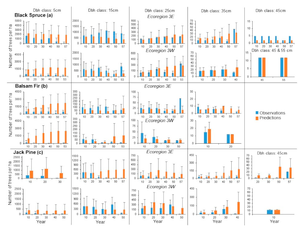
Agreement for dbh class distributions for black spruce in Ecoregion 3E was relatively high between mean observed and predicted stand densities for several years and dbh classes (Figure 6a). Differences between mean observations and predictions were generally more pronounced in older years and large dbh classes. However, for most dbh classes and years, the standard deviations between observations and predictions largely overlapped. For the 45 cm dbh class, the absence of standard deviations was the result of lack of variation in the observed and predicted numbers of trees. These results are consistent with the similarity coefficients computed at the plot scale, which indicated a gradual decrease over year, but with relatively high coefficients in the first 40 years (Figure 7). Differences between mean observed and predicted stand densities in Ecoregion 3W were larger than those in Ecoregion 3E for the 5 cm dbh class, but agreement was relatively high for the 15, 25 and 35 cm dbh classes for most years (Figure 6a). For the 45 and 55 cm dbh classes, observed and predicted mean stand densities at years 45 and 55 were the same, which explains the absence of standard deviations. The similarity coefficients were generally smaller than those in Ecoregion 3E, particularly in the first few years, and were also characterized by a pattern of decrease over time (Figure 7). When analyzed by combining plots, years and dbh classes, results indicated that 47.3 and 61.2% of the differences between observed and predicted stand densities were less than 100 trees ha⁻¹ for ecoregions 3E and 3W, respectively (

Table 8. Percentages of plots in different classes (20 trees ha⁻¹) of differences between observed and predicted stand densities (trees ha⁻¹) in Ecoregion 3E, northern Ontario, Canada.

Species	Classes of Differences between Observations and Predictions in Stand Density
	0	1–20	21–40	41–60	61–80	81–100	101–120	121–140	141–160	161–180	181–200	>200
Black spruce	16.1	11.7	7.8	4.3	4.1	3.3	1.9	2.5	2	1.6	2	42.8
Balsam fir	22.2	16.2	7	2.6	2.8	3.8	1.2	1.9	2.3	1.7	1.4	37
Jack pine	32.7	22.6	11.3	8.7	5.3	2.9	0.2	2.4	1.2	0.5	1.7	10.6
White birch	29.3	20.3	11.8	4.9	6	3.4	2.3	2.1	1.6	1.1	1.1	16.2
White spruce	36.7	8.3	31.7	6.7	10	1.7	1.7	-	-	1.7	-	1.7
Balsam poplar	31.9	27.2	13.3	6.6	5.9	3.3	2	1.5	1.8	1.2	0.7	14.5
Trembling aspen	28.2	14.3	11.8	5.5	7.1	4.7	3	2.8	1.7	2.9	1.1	17
American larch	29.8	36.7	8.2	5.6	3.9	3	1.5	0.9	0.6	0.9	0.9	7.9

and

Table 9. Percentages of plots in different classes (20 trees ha⁻¹) of differences between observed and predicted stand densities (trees ha⁻¹) in Ecoregion 3W in northern Ontario, Canada.

Species	Classes of Ranges of Differences between Observations and Predictions in Stand Density
	0	1–20	21–40	41–60	61–80	81–100	101–120	121–140	141–160	161–180	181–200	>200
Black spruce	26.4	10.4	11.4	3.5	5.6	3.9	2.2	2.4	1.9	1.4	1.4	29.5
Balsam fir	33.8	10.9	7.4	3.1	3.8	2.1	0.7	1.9	0.9	1.3	1.6	32.5
Jack pine	27.5	8	9.8	3.5	7.1	5.8	1.7	4.5	1.8	2	3	25.3
White birch	37.8	16.3	14.9	3.7	4.8	3.5	1.2	2.1	1	1.3	0.5	12.9
White spruce	58.6	26.9	9.6	1.3	1.1	0.4	0.2	1.1	0.4	-	-	0.2
Balsam poplar	56.6	15.9	13.1	2.8	5.6	3.4	0.9	0.9	-	0.3	-	0.3
Trembling aspen	36.9	13.6	12.7	3.8	4.9	5.3	2.2	2.5	1.8	1.9	2	12.4
American larch	66.7	22.2	6.7	-	-	-	2.2	-	-	2.2	-	-

). Differences greater than 100 trees ha⁻¹ may appear considerable, but, in reality, they are less important when adjusted to sample plot area That is, a difference of 100 trees ha⁻¹ means a difference of 4 trees in a 400 m² sample plot. Differences greater than 100 trees ha⁻¹ were observed for sample plots combined with years and dbh classes with high densities.

For balsam fir in Ecoregion 3E, relatively good agreements were observed between mean observed and predicted densities for some years in the 15, 25 and 35 cm dbh classes (Figure 6b). Low agreement was evident for all years for the 5 cm dbh class. For year 50 for the 35 cm dbh class, ZELIG-CFS predicted the presence of 7 trees ha⁻¹, but none were present in the observations. However, 7 years later (year 57), trees were present in this dbh class, suggesting an error in the observation data set. No differences were observed between 22% of the observed and predicted stand densities and 37% were greater than 200 trees ha⁻¹ (Table 8). Percent differences decreased gradually from the lowest (1–20 trees ha⁻¹) to the highest (181–200 trees per plot) density classes. Except for 11 years, the similarity coefficients were higher than 0.50 (Figure 7). Differences between observed and predicted mean stand densities were more pronounced in Ecoregion 3W than 3E, particularly for the 5 and 15 cm dbh classes (Figure 6b), which resulted in lower similarity coefficients (Figure 7). ZELIG-CFS predicted high densities for both dbh classes, but observations indicated that few trees were present. It is possible that errors in the observation data set may be the cause of the disparity. Despite the large differences between observations and predictions, agreement was high in many instances. The absence of differences between observations and predictions were evident for 33.8% of the combinations of sample plots, years and dbh classes, 33.7% of the differences varied between 1 and 200 trees ha⁻¹ and 32.5% of the differences were greater than 200 trees ha⁻¹ (Table 8).

Larges differences between mean observed and predicted stand densities were observed for jack pine in Ecoregion 3E for most years in each dbh class (Figure 6c). However, the percentages of differences between observed and predicted stand densities suggest that the large differences were caused by only a relatively small number of combinations of sample plots, years and dbh classes in the results (Table 8). As much as 32.7% of the differences between observed and predicted stand densities were less than 1 tree ha⁻¹, 56.8% of them were between 1 and 200 trees ha⁻¹ and only 10.6% of them were greater than 200 trees ha⁻¹ (Table 8). The relatively high percentage of the absence of differences between observations and predictions may explain the occurrence of relatively high similarity coefficients (Figure 7). Except for the 5 cm dbh class, differences between observed and predicted stand densities were smaller for Ecoregion 3W than for 3E (Figure 6c). Substantial overlaps between the standard deviations of observations and predictions suggested that agreement was high in several instances. As much as 27.5% of the differences between observations and predictions were negligible, 47.2% were between 1 and 200 stems ha⁻¹, and 25.3% were greater than 200 stems ha⁻¹ (Table 9). Similarity coefficients were greater than 0.50 for 13 years over a total of 40 years (Figure 7).

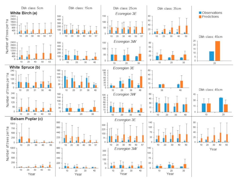
The patterns of mean dbh class distribution for white birch in Ecoregion 3E indicated high agreement between observations and predictions for some years and dbh classes (Figure 8a). Substantial differences were observed for the older years in the 5, 15 and 35 cm dbh classes and only for year 57 in the 25 cm dbh class. Large overlaps in the standard deviations between observations and predictions indicated agreement was high in several cases: differences between observations and predictions did not differ for 29.3% of the combinations of sample plots, years and dbh classes and only 16.2% of them were greater than 200 trees ha⁻¹ (Table 8). Similarity coefficients were relatively low for most years (Figure 7). Results for Ecoregion 3W differed considerably from those for Ecoregion 3E (Figure 8a). Most of the large differences between mean observed and predicted stand densities were observed in the older years for most dbh classes, except for the 25 cm dbh class. As suggested by the large overlaps between the standard deviations of observations and predictions, agreement was high for many combinations of sample plots, years and dbh classes: no difference between observed and predicted stand densities were observed in 37.8% of the cases and only 12.9% had differences greater than 200 trees ha⁻¹ (Table 9). Most of the similarity coefficients were smaller than 0.50 (Figure 7).

For white spruce in Ecoregion 3E, agreement between observed and predicted mean stand densities were high for most dbh classes and years (Figure 8b). There were no differences between observed and predicted stand densities for 36.7% of the combinations of sample plots, years and dbh class distributions and only 1.7% of them were greater than 200 trees ha⁻¹ (Table 8). The similarity coefficients were all greater than 0.60 (Figure 7). Except for the 5 cm dbh class, agreement between observed and predicted stand densities was high for Ecoregion 3W (Figure 8b). In general, differences between observed and predicted stand densities were smaller than those in Ecoregion 3E (Figure 8b): 58.6% of the differences between observed and predicted stand densities were negligible and only 0.2% of them were higher than 200 trees ha⁻¹. The similarity coefficients were all greater than 0.60.

Differences between observed and predicted mean stand densities were large for balsam poplar in Ecoregion 3E for most of the dbh classes and years (Figure 8c). Relatively high agreement was observed only for year 10 in the 5, 15 and 25 cm dbh classes. However, despite the pronounced differences in the mean densities, the results at the sample plot scale and by dbh class and year indicated that 31.9% of observed stand densities coincided with the predicted densities and 14.5% of them were higher than 200 trees ha⁻¹ (Table 8). The similarity coefficients were low beyond year 20 (Figure 7). The comparison of mean stand densities for Ecoregion 3W indicated better agreement than that for Ecoregion 3E between observations and predictions (Figure 8c). This can be seen in the percent differences between observed and predicted stand densities (Table 9). Only 0.3 % of the differences between observed and predicted stand densities were higher than 200 trees ha⁻¹ and as much as 56.6% of them were negligible. The similarity coefficients were all greater than 0.60, except for years 31 and 33 (Figure 7).

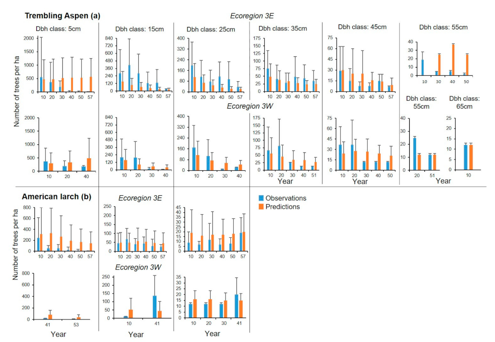
In Ecoregion 3E, observed and predicted mean stand densities for trembling aspen differed considerably in the 5, 15, 25 and 55 cm dbh classes for nearly all years (Figure 9a). Relatively high agreements between observations and predictions were observed for years 10 and 20 in the 5 cm class and for most years in the 35 and the 45 cm dbh classes. Similar to the other species, there were large overlaps between the standard deviations for most combinations of sample plots, years and dbh classes that can be associated with several high agreements between observations and predictions. As much of 28.2% of the differences between observed and predicted stand densities did not differ and 54.9% of the percent differences were between 1 and 200 trees ha⁻¹ (Table 8). Most of the similarity coefficients were smaller than 0.50 (Figure 7). Higher agreements between observed and predicted mean stand densities were observed for Ecoregion 3W than that for 3E for most years and dbh classes, except for year 30 in the 15, 25 and 45 cm dbh classes, year 40 in the 5, 15, 35 and 45 cm dbh classes (Figure 9a). Despite the large departures, agreement was high between observed and predicted stand densities in many cases (Table 9). There were no differences between observed and predicted stand densities for 36.9% of the combinations of sample plots, years and dbh classes and only 12.4 of them were greater than 200 trees ha⁻¹. Similarity coefficients were higher than 0.40 until year 35, except for years 29 and 33, then gradually declined, except for year 46 (Figure 7).

For American larch, agreement was high between observed and predicted mean stand densities in Ecoregion 3E, except for years 20 to 57 in the 5 cm dbh class and years 10, 20, 40 and 50 in the 25 cm dbh class (Figure 9b). As much as 29.8% of the differences between observed and predicted stand densities were negligible and only 7.9% of them were greater than 200 trees ha⁻¹ (Table 8). Most similarity coefficients were greater than 0.40 for most years (Figure 5d). American larch was less present in Ecoregion 3W (Figure 9b). Agreement was high between mean observations and predictions only in the 25 cm dbh class. As much of 66.7% of the differences between observations and predictions were negligible and 11.1% of them were higher than 21 trees ha⁻¹ (Table 9). These results can be associated with relatively high similarity coefficients (Figure 7).

4. Discussion

As far as could be evaluated from the literature covering recent decades, support is high for the existence of forest gap dynamics in boreal forests [10,11,12,13,14,15]. The present study is, however, one of the rare efforts, such as the study by [62], that have evaluated the performance of a gap model using extensive long-term historical data for forest types varying substantially in species composition. This issue was raised by [26] who highlighted the need for using extensive data sets for evaluating the performance of gap models to avoid bias toward some species or ages. The factors that must be considered in the comparison of the predictions of gap models with observed stand data can be classified in three groups [29]: (1) degree to which the environmental site variables used in the simulations are accurate and representative of the field conditions; (2) extent to which observed data, which may originate from inventory surveys, represent the forests under examination; and (3) extent to which potential successional changes and management activities are taken into account. As previously mentioned, ZELIG-CFS is a semi-mechanistic model that includes basic environmental site variables for the simulations, including monthly mean temperatures and precipitations and basic soil texture, in the initialization files. For climatic and soil texture data, the estimates were fairly accurate and representative of field conditions at the sample plot scale. The application BioSIM [48], which was used to estimate monthly mean temperatures and precipitations, is based on interpolations from regional weather stations by taking each sample plot’s latitudes, longitudes and altitudes into account to the coordinates of each sample plot. Soil texture data were obtained from soil maps and basic description of soil characteristics for each sample plot. The historical long-term sample plot data set used in this study originated from a databank developed and maintained by the NDMNRF Growth and Yield Program and the measurements were conducted by ministry staff or forest companies mentioned above, which provides a strong confidence in the validity of the measurements. Of course, measurement errors were possibly made at the time of measurements or introduced in inventory reports, but it is unlikely that they were sufficient to invalidate a large proportion of the data set. The third factor was less relevant for the present study, as very few sample plots were subject to management activities, such as partial cuts. However, since remeasurement data spanned relatively long periods of time, the successional pathways were likely well captured.

The patterns of change in predicted mean basal area over relatively long periods were consistent with observations for most species in both ecoregions, except for trembling aspen in Ecoregion 3E. The simultaneous occurrences of fluctuations in observations and predictions for several years suggest that the patterns of predicted mortality and regeneration were generally well captured by ZELIG-CFS. Relatively small fluctuations from years to years are normal in the course of stand dynamics when observations and predictions from several sample plots are assembled and analyzed. However, large fluctuations were observed in mean basal area in several cases within very short periods, such as those in Ecoregion 3W from years 25 to 27 for trembling aspen and from years 43 to 50 for balsam fir and, in Ecoregion 3W, from years 42 to 44 for black spruce. These rapid changes might have been caused by some errors in the records.

ZELIG-CFS generally overpredicted stand density, particularly in the small dbh classes, but, similarly to the results by [63,64], predicted that the differences between observed and predicted stand densities tended to decrease with increasing dbh class for most species. This pattern can be explained by high regeneration rates predicted by ZELIG-CFS for several sample plots, which increased predicted stand density in the smallest dbh classes. Then, differences between observed and predicted densities were reduced over time, as young trees died in the years following their establishment. Thus, our results suggest that ZELIG-CFS consistently predicted small tree mortality in the years after their establishment. However, overprediction of regeneration did not occur consistently in all sample plots. As indicated above, large overlaps in the standard deviations were evident between observed and predicted mean densities, which could be associated with many cases of agreement between observed and predicted stand densities and high similarity coefficients. Nevertheless, these patterns do not indicate that ZELIG-CFS consistently failed to realistically predict regeneration establishment. Large differences between observations and predictions do not necessarily indicate that a model does not adequately represent mechanisms or failed to make realistic predictions [29]. A good example of this statement is the modelling of regeneration [37]. ZELIG-CFS requires as input the potential numbers of seedlings that might germinate every year and then randomly selects the number of seedlings that will appear by considering the site conditions, including understory light conditions and soil moisture. This modelling procedure is biologically consistent and is an optimal solution given the lack of experimental data. Many surveys have been conducted to estimate regeneration establishment in forest ecosystems, but they are just a picture at one point in time and, as such, do not capture potential annual variations and early seedling survival. This may partially explain some of the differences between observed and predicted stand densities in small dbh classes. Despite consistent predictions of regeneration, these results suggest that there is a need to gain a better understanding on the different stages of regeneration, including seed germination, seedling growth and mortality and transition from seedlings to trees to improve the modelling of regeneration. However, the fact that differences between observed and predicted stand densities diminished over time for some species suggests that ZELIG-CFS consistently and realistically predicted tree mortality, which is a complex process involving interactive effects of several factors [65,66,67]. The prediction of mortality may be more difficult for some species. For instance, mortality in paper birch stands may be important throughout all its life, unless suppressed trees are released early [68].

Black spruce is a dominant species in both ecoregions. It was present in 94 and 97% of the sample plots in ecoregions 3E and 3W, respectively, and was characterized by high basal areas and stand densities for nearly all years and dbh classes. These results can be related to the ecological properties of black spruce. Black spruce grows well in a wide range of ecological conditions, including organic and mineral soils, cold and high temperatures and low and high precipitation [69,70]. Additionally, as a shade-tolerant species, it grows well in pure and mixed forests and its seedlings may grow in as little as one-tenth of understory sunlight [71]. Black spruce occupies a special niche as a late succession species where most succession pathways converge in the boreal forest of Ontario [6].

Balsam fir was less present in terms of basal area and stand density than black spruce in both ecoregions, but was found in 65 and 48% of sample plots in ecoregions 3E and 3W, respectively. It has growing requirements similar to those of black spruce with respect to temperature and precipitation [71,72] and is a late successional species that may maintain itself in mixed forests with black spruce, white spruce and white birch for long periods in the absence of disturbances, particularly fires [71]. Additionally, its seedlings can grow well under poor understory light conditions for long periods, but respond vigorously to increases in understory light conditions following gap openings [71]. Its development in mixed stands and longevity was consistently represented by ZELIG-CFS.

Basal area for jack pine was similar in both ecoregions for approximately the first 20 years of the simulations. While there was a pattern of slight increase in basal area in Ecoregion 3W, it decreased in Ecoregion 3E. Jack pine occurred more often in Ecoregion 3W than in 3E. The decline in Ecoregion 3E may be explained by the fact that jack pine is a transient species that is eventually replaced by late successional species, such as black spruce or balsam fir, that better tolerate understory shade conditions [69]. Additionally, as jack pine is a shade-intolerant species, its seedlings do not grow well in low-light conditions [70,71]. Two possible reasons for its more frequent occurrence in Ecoregion 3W than 3E are: first, more stands were in a state of successional transition in Ecoregion 3E. Second, soil conditions were more favorable for jack pine in Ecoregion 3W. The best soil conditions for jack pine are well drained or dry loamy acidic sands, such as those Ecoregion 3W [38,69]. Large areas in Ecoregion 3E have calcareous fine texture soils, including silts or clay [38], which are less favorable for jack pine.

White birch was present in 58 and 50% of the sample plots in ecoregions 3E and 3W, respectively. It is a shade-intolerant species that can grow as a minor component in openings of mixed late successional forests [18,69]. White birch presented patterns similar to those of jack pine with respect to basal area in both ecoregions: a decline in Ecoregion 3E, but an increase in 3W, despite fluctuations. Again, more stands were in a state of transition in Ecoregion 3E than 3W, reducing white birch occurrence. Another explanation is that it may grow as codominant with trembling aspen, black spruce, white spruce, jack pine and balsam fir, but rarely is a late successional species [69]. The presence of white birch in mixed old forests may be associated with its robust capacity to produce and propagate seedlings on different soil conditions [68,72]. The fact that its seedlings can develop under 50% of full sunlight probably contributes to its higher densities in Ecoregion 3W [65], contrary to jack pine. The effect of differences in soil properties and temperature and precipitation conditions between both ecoregions may not explain differences in basal area development in both ecoregions. White birch usually grows on well-drained sandy loams and is adapted to wide variations in temperature and precipitation [70].

White spruce was present in 4 and 33% of the sample plots in ecoregions 3E and 3W, respectively, but stand density was generally higher in Ecoregion 3E than 3W. Its ecological properties do not explain the differences of its development between ecoregions. White spruce can grow in large variations of climatic conditions and soil properties, including acid or calcareous loams and clays and wet or dry sites [69]. As suggested by the basal area and stand density values relative to the other species, it is a minor component in most stands surveyed in the present study. White spruce can grow in successional transitions with trembling aspen and paper birch that may eventually become pure stands, but may also reach a late successional status with other boreal species, such as black spruce, which explains why it was found in so many mixed stands for both observations and predictions [69]. In particular, white spruce may benefit from the presence of trembling aspen [73].

Despite fluctuations, basal area and stand density for balsam poplar were generally higher in Ecoregion 3E than 3W and this species was present in 37 and 22% of the sample plots in the respective ecoregions. Balsam poplar is a low shade-tolerant species that grows in a wide range of climatic conditions and, although it grows best on moist sites, it can tolerate dry sites [69]. It is an early successional species that colonizes disturbed wet sites that will generally lead to mixed forests [69]. The fine textured soils with silts or clay likely explains its greater presence and development of basal area in Ecoregion 3E. These soils retain more water than the generally well drained soils in Ecoregion 3W.

Trembling aspen was the species with the lowest agreement between observed and predicted basal areas and stand densities in both ecoregions. It is a pioneer species that grows well in various cold boreal climatic conditions and can colonize disturbed sites with poor soils, including bare soils, but requires moist conditions to grow well [69,70,74]. It is widely distributed in North America [70], but was found in only 26 and 57% of the sample plots in this study, which may indicate that sample plots were not evenly disturbed, considering its capacity to invade disturbed sites. It is also possible that, as a shade-intolerant species, its seedlings normally cannot grow below its own canopy [74], unless there are gaps caused by disturbances, such as windthrow, as observed in aspen-white spruce forests [74,75]. An explanation for the large differences between observations and predictions may be that ZELIG-CFS did not well capture the complexity of the mortality process for this species in the region. It seems that mortality does not occur on a regular basis for trembling aspen, as there may be episodes of high mortality rates in young stands caused by competition for light from shade-tolerant dominant species that will replace them in the course of succession, drought conditions or intensive browsing [70,76].

American larch was a minor species in the data set. It was present in 6 and 5% of the sample plots in ecoregions 3E and 3W, respectively, and its basal area and stand density were smaller than those for most species. The simulation results agree with what has been observed for this species. In the boreal forest of Ontario, American larch may grow alone or with other species, including black spruce, balsam fir, white spruce, white birch or trembling aspen, but remains in small proportions in mixed stands [69]. The reasons that may explain why it was found in only a few sample plots include its specific site requirements and its shade intolerance to the extent that its seedlings cannot grow under its own canopy. Its best growth conditions occur on moist to poorly drained soils, including acid swamps, bogs, or muskegs, but it can also be found in moist areas along streams or lakes [65].

5. Conclusions

The evaluation of the performance of the succession model ZELIG-CFS for various boreal mixed forest types in northern Ontario indicated that it generally predicted the development of most species well when compared with historical data sets and also captured the effects of differences in species-specific ecological properties. Some important discrepancies between observations and predictions could be partly explained by potential errors in the data sets. However, as with any model, the representations of some mechanisms could be improved. The major one involves the dynamics of the transitions from seedling to sapling to tree stages. For most species, understanding about these transitions remains sparse as forest ecosystem studies focus on young or mature forests. Even with current knowledge or information, the modelling of some processes, such as regeneration, competitive effects or temperature and precipitation variation, will always include some degree of uncertainty. Most available models provide deterministic results. Including uncertainty algorithms to provide uncertainty estimates in model predictions might be helpful.

References

1. Pan, Y.; Birdsey, R.A.; Fang, J.; Houghton, R.; Kauppi, P.E.; Kurz, W.A.; Phillips, O.L.; Shvidenko, A.; Lewis, S.L.; Canadell, J.G.; et al. A large and persistent carbon sink in the world’s forests. Science 2011, 333, 988–993. [Google Scholar] [CrossRef] [PubMed] [Green Version]
2. Venier, L.A.; Thompson, I.D.; Fleming, R.; Malcolm, J.; Aubin, I.; Trofymow, J.A.; Langor, D.; Sturrock, R.; Patry, C.; Outerbridge, R.O.; et al. Effects of natural resource development on the terrestrial biodiversity of Canadian boreal forests. Environ. Rev. 2014, 22, 457–490. [Google Scholar] [CrossRef]
3. Brandt, J.P.; Flannigan, M.D.; Maynard, D.G.; Thompson, I.D.; Volney, W.J.A. An introduction to Canada’s boreal zone: Ecosystem processes, health, sustainability, and environmental issues. Environ. Rev. 2013, 21, 207–226. [Google Scholar] [CrossRef]
4. Gauthier, S.; Bernier, P.; Kuuluvainen, T.; Shvidenko, A.Z.; Schepaschenko, D.G. Boreal forest health and global change. Science 2015, 349, 819–822. [Google Scholar] [CrossRef] [PubMed]
5. Pohjanmies, T.; Triviño, M.; Le Tortorec, E.; Mazziotta, A.; Snäll, T.; Mönkkönen, M. Impacts of forestry on boreal forests: An ecosystem services perspective. Ambio 2017, 46, 743–755. [Google Scholar] [CrossRef] [PubMed]
6. Drescher, M.; Perera, A.H.; Buse, L.J.; Arnup, R.; Bowling, C.; Etheridge, D.; Niznowski, G.; Ride, K.; Vasiliauskas, S. Boreal Forest Succession in Ontario: An Analysis of the Knowledge Space; Forest Research Report No. 171; Ontario Forest Research Institute: Sault Ste. Marie, ON, Canada, 2008; 59p. [Google Scholar]
7. Taylor, A.R.; Chen, H.Y.H.; VanDamme, L. A review of forest succession models and their suitability for forest management planning. For. Sci. 2008, 55, 23–36. [Google Scholar]
8. Finegan, B. Forest succession. Nature 1984, 312, 109–114. [Google Scholar] [CrossRef]
9. Bazzaz, F.A. Plants in Changing Environments; Cambridge University Press: Cambridge, UK, 1996; pp. 4–5. ISBN 9-780521-398435. [Google Scholar]
10. Kuuluvainen, T. Gap disturbance, ground microtopography, and the regeneration dynamics of boreal coniferous forests in Finland: A review. Ann. Zool. Fennici 1994, 31, 35–51. [Google Scholar]
11. Kneeshaw, D.D.; Bergeron, Y. Canopy gap characteristics and tree replacement in the southeastern boreal forest. Ecology 1998, 81, 1500–1516. [Google Scholar] [CrossRef]
12. Pham, A.T.; De Grandpré, L.; Gauthier, S.; Bergeron, Y. Gap dynamics and replacement patterns in gaps of the northeastern boreal forest of Quebec. Can. J. For. Res. 2004, 34, 353–364. [Google Scholar] [CrossRef]
13. Hill, S.B.; Mallik, A.U.; Chen, H.Y.H. Canopy gap disturbance and succession in trembling aspen dominated boreal forests in northeastern Ontario. Can. J. For. Res. 2005, 35, 1942–1951. [Google Scholar] [CrossRef]
14. Caron, M.-N.; Kneeshaw, D.D.; Grandpré, L.; Kauhanen, H.; Kuuluvainen, T. Canopy gap characteristics and disturbance dynamics in old-growth Picea abies stands in northern Fennoscandia: Is the forest in quasi-equilibrium. Ann. Bot. Fennici 2009, 46, 251–262. [Google Scholar] [CrossRef] [Green Version]
15. Barrette, M.; Bélanger, L.; De Grandpré, L.; Royo, A.A. Demographic disequilibrium caused by canopy gap expansion and recruitment failure triggers forest cover loss. For. Ecol. Manag. 2017, 401, 117–124. [Google Scholar] [CrossRef]
16. Sernander, R. Granskär och Fiby urskog. En studie över stormluckornas och marbuskarnas betydelse i den svenska granskogens regeneration [The primitive forests of Granskär and Fiby. A study of the part played by storm gaps and dwarf trees in the regeneration of the Swedish spruce forest, English summary p. 220-227]. Acta Phytogeogr. Suec. 1936, 8, 1–232. [Google Scholar]
17. Yamamoto, S.-I. Forest gap dynamics and tree regeneration. J. For. Res. 2000, 5, 223–229. [Google Scholar] [CrossRef]
18. McCarthy, J. Gap dynamics of forest trees: A review with particular attention to boreal forests. Environ. Rev. 2001, 9, 1–59. [Google Scholar] [CrossRef]
19. Chen, H.Y.H.; Taylor, A.R. A test of ecological succession hypotheses using 55-year time-series data for 361 boreal forest stands. Global Ecol. Biogeogr. 2012, 21, 441–454. [Google Scholar] [CrossRef]
20. Larocque, G.R. Forest models. In Ecological Models. Volume 2 of Encyclopedia of Ecology; Jøgensen, S.E., Fath, B.D., Eds.; Elsevier: Oxford, UK, 2008; pp. 1663–1673. [Google Scholar]
21. Botkin, D.B.; Janak, J.F.; Wallis, J.R. Some ecological consequences of a computer model of forest growth. J. Ecol. 1972, 60, 849–872. [Google Scholar] [CrossRef] [Green Version]
22. Risch, A.C.; Heiri, C.; Bugmann, H. Simulating structural forest patterns with a forest gap model: A model evaluation. Ecol. Modell. 2005, 181, 161–172. [Google Scholar] [CrossRef]
23. Wehrli, A.; Zingg, A.; Bugmann, H.; Huth, A. Using a forest patch model to predict the dynamics of stand structure in Swiss mountain forests. For. Ecol. Manag. 2005, 205, 149–167. [Google Scholar] [CrossRef]
24. Larocque, G.R.; Shugart, H.H.; Xi, W.; Holm, J.A. Forest succession models. In Ecological Forest Management Handbook; Larocque, G.R., Ed.; CRC Press: Boca Raton, FL, USA, 2016; pp. 179–221. [Google Scholar]
25. Didion, M.; Kupferschmid, A.D.; Lexer, M.J.; Rammer, W.; Seidl, R.; Bugmann, H. Potentials and limitations of using large-scale forest inventory data for evaluating forest succession models. Ecol. Modell. 2009, 220, 133–147. [Google Scholar] [CrossRef]
26. Bugmann, H.K.M.; Wullschleger, S.D.; Price, D.T.; Ogle, K.; Clark, D.F.; Solomon, A.M. Comparing the performance of forest gap models in North America. Clim. Chang. 2001, 51, 349–388. [Google Scholar] [CrossRef]
27. Ngugi, M.R.; Botkin, D.B. Validation of a multispecies forest dynamics model using 50-year growth from Eucalyptus forests in eastern Australia. Ecol. Modell. 2011, 222, 3261–3270. [Google Scholar] [CrossRef]
28. Schuman, J.K.; Shugart, H.H.; Krankina, O.N. Testing individual-based models of forest dynamics: Issues and an example from the boreal forests of Russia. Ecol. Modell. 2014, 293, 102–110. [Google Scholar] [CrossRef]
29. Badeck, F.-W.; Lischke, H.; Bugmann, H.; Hickler, T.; Honninger, K.; Lasch, P.; Lexer, M.J.; Mouillot, F.; Schaber, J.; Smith, B. Tree species composition in European pristine forests: Comparison of stand data to model predictions. Clim. Chang. 2001, 51, 307–347. [Google Scholar] [CrossRef]
30. Stadt, K.J.; Huston, C.; Coates, K.D.; Feng, Z.; Date, M.R.T.; Lieffers, V.J. Evaluation of competition and light estimation indices for predicting diameter growth in mature boreal mixed forests. Ann. For. Sci. 2007, 64, 477–490. [Google Scholar] [CrossRef] [Green Version]
31. Thorpe, H.C.; Vanderwel, M.C.; Fuler, M.M.; Thomas, S.C.; Caspersen, J.P. Modelling stand development after partial harvests: An empirically based, spatially explicit analysis for lowland black spruce. Ecol. Model. 2010, 221, 256–267. [Google Scholar] [CrossRef]
32. Beaudet, N.; Harvey, B.D.; Messier, C.; Coates, K.D.; Poulin, J.; Kneeshaw, D.D.; Brais, S.; Bergeron, Y. Managing understory light conditions in boreal mixedwoods through variation in the intensity and spatial patternof harvest: A modelling approach. For. Ecol. Manage. 2011, 261, 84–94. [Google Scholar] [CrossRef] [Green Version]
33. Rasche, L.; Fahse, L.; Zingg, A.; Bugmann, H. Enhancing gap model accuracy by modeling dynamic height growth and dynamic maximum tree height. Ecol. Modell. 2012, 232, 133–143. [Google Scholar] [CrossRef]
34. Brazhnik, K.; Shugart, H.H. SIBBORK: A new spatially-explicit gap model for boreal forest. Ecol. Modell. 2016, 320, 182–196. [Google Scholar] [CrossRef] [Green Version]
35. Bose, A.K.; Harvey, B.D.; Coates, K.D.; Brais, S.; Bergeron, Y. Modelling stand development after partial harvesting in boreal mixedwoods of eastern Canada. Ecol. Modell. 2015, 300, 123–136. [Google Scholar] [CrossRef]
36. Maleki, K.; Gueye, M.A.; Lafleur, B.; Leduc, A.; Bergeron, Y. Modeling post-disturbance successional dynamics of the Canadian boreal mixedwoods. Forests 2020, 11, 3. [Google Scholar] [CrossRef] [Green Version]
37. Larocque, G.R.; Archambault, L.; Delisle, C. Development of the gap model ZELIG-CFS to predict the dynamics of North American mixed forest types with complex structures. Ecol. Modell. 2011, 222, 2570–2583. [Google Scholar] [CrossRef]
38. Crins, W.J.; Gray, P.A.; Uhlig, P.W.X.; Wester, M.C. The Ecosystems of Ontario, Part I: Ecozones and Ecoregions; Inventory, Monitoring and Assessment, SIB TER IMA, TR-01; Ontario Ministry of Natural Resources: Peterborough, ON, Canada, 2009; 71p. [Google Scholar]
39. Urban, D.L. A Versatile Model to Simulate Forest Pattern: A User’s Guide to ZELIG Version 1.0; University of Virginia: Charlottesville, Virginia, 1990. [Google Scholar]
40. Urban, D.L. Using model analysis to design monitoring programs for landscape management and impact assessment. Ecol. Appl. 2000, 10, 1820–1832. [Google Scholar] [CrossRef]
41. Urban, D.L.; Bonan, G.B.; Smith, T.M.; Shugart, H.H. Spatial applications of gap models. For. Ecol. Manag. 1991, 42, 95–110. [Google Scholar] [CrossRef]
42. Yang, X.; Miller, D.R.; Montgomery, M.E. Vertical distributions of canopy foliage and biologically active radiation in a defoliated/refoliated hardwood forest. Agric. For. Meteorol. 1993, 67, 129–146. [Google Scholar] [CrossRef]
43. Yang, X.; Witcosky, J.J.; Miller, D.R. Vertical overstory canopy architecture of temperate deciduous hardwood forests in the eastern United States. For. Sci. 1999, 45, 349–358. [Google Scholar]
44. Baldwin, V.C., Jr.; Peterson, K.D.; Burkhart, H.E.; Amateis, R.L.; Doughterty, P.M. Equations for estimating loblolly pine branch and foliage weight and surface area distributions. Can. J. For. Res. 1997, 27, 918–927. [Google Scholar] [CrossRef]
45. Larocque, G.R. Coupling a detailed photosynthetic model with foliage distribution and light attenuation functions to compute daily gross photosynthesis in sugar maple (Acer saccharum Marsh.) stands. Ecol. Modell. 2002, 148, 212–232. [Google Scholar] [CrossRef]
46. Elzein, T.; Larocque, G.R.; Sirois, L.; Arseneault, D. Comparing the predictions of gap model with vegetation and disturbance data in south-eastern Canadian mixed forests. For. Ecol. Manag. 2020, 455, 1–12. [Google Scholar] [CrossRef]
47. Holm, J.A.; Shugart, H.H.; Van Bloem, S.J.; Larocque, G.R. Gap model development, validation, and application to succession of secondary subtropical forests of Puerto Rico. Ecol. Modell. 2012, 233, 70–82. [Google Scholar] [CrossRef]
48. Régnière, J.; Saint-Amant, R.; Béchard, A.; Moutaoufik, A. BioSIM 11 User’s Manual; Update of Inf. Rep.LAU-X-137; Natural Resources Canada, Canadian Forest Service: Gatineau, QC, Canada, 2017. [Google Scholar]
49. Groot, A. Stand and Site Conditions Associated with Abundance of Black Spruce Advance Growth in the Northern Clay Section of Ontario; Inf. Rep.O-X-358; Department of the Environment, Canadian Forestry Service, Great Lakes Forest Research Centre: Sault Ste. Marie, ON, Canada, 1984; p. 14. [Google Scholar]
50. Groot, A. Regeneration and Surface Condition Trends Following Forest Harvesting on Peatlands; NODA/NFP Tech. Rep. TR-26; Natural Resources Canada, Canadian Forest Service, Great Lakes For. Cen.: Sault Ste. Marie, ON, Canada, 1996; p. 12. [Google Scholar]
51. Harvey, B.D.; Bergeron, Y. Site patterns of natural regeneration following clear-cutting in northwestern Quebec. Can. J. For. Res. 1989, 19, 1458–1469. [Google Scholar] [CrossRef]
52. Walsh, S.A.; Wickware, G.M. Stand and Site Conditions Associated with the Occurrence and Distribution of Black Spruce Advance Growth in North Central Ontario; COFRDA Rep. 3309, Tech Rep. 24; Forestry Canada, Ontario Region: Sault Ste. Marie, ON, Canada; Northwestern Ontario Forest Technology Development Unit, Ontario Ministry of Natural Resources: Thunder Bay, ON, Canada, 1991. [Google Scholar]
53. Arnup, R.W. Stand and Site Conditions Associated with the Abundance and Distribution of Black Spruce and Balsam Fir Advance Growth in Northeastern Ontario; NODA/NFP Tech. Rep. TR-29; Natural Resources Canada, Canadian Forest Service, Great Lakes Forestry Centre: Sault Ste. Marie, ON, Canada, 1996; p. 25. [Google Scholar]
54. Brais, S.; Harvey, B.D.; Bergeron, Y.; Messier, C.; Greene, D.; Belleau, A.; Paré, D. Testing forest ecosystem management in boreal mixedwoods of northwestern Quebec: Initial response of aspen stands to different levels of harvesting. Can. J. For. Res. 2004, 34, 431–446. [Google Scholar] [CrossRef] [Green Version]
55. Man, R.; Rice, J.A.; MacDonald, G.B. Five-year light, vegetation, and regeneration dynamics of boreal mixedwoods following silvicultural treatments to establish productive aspen-spruce mixtures in northeastern Ontario. Can. J. For. Res. 2010, 40, 1529–1541. [Google Scholar] [CrossRef]
56. Man, R.; Rice, J.A.; Freeman, L.; Stuart, S. Effects of pre- and post-harvest spray with glyphosate and partial cutting on growth and quality of aspen regeneration in a boreal mixedwood forest. For. Ecol. Manag. 2011, 262, 1298–1304. [Google Scholar] [CrossRef]
57. Man, R.; Rice, J.A.; MacDonald, G.B. Performance of planted spruce and natural regeneration after pre- and post- harvest spraying with glyphosate and partial occurring on an Ontario (Canada) boreal mixedwood site. Forestry 2013, 86, 475–480. [Google Scholar] [CrossRef] [Green Version]
58. Larouche, C.; Ruel, J.-C.; Lussier, J.-M. Factors affecting northern white-cedar (Thuja occidentalis) seedling establishment and early growth in mixedwood stands. Can. J. For. Res. 2011, 41, 568–582. [Google Scholar] [CrossRef]
59. Vanclay, J.K. Modelling Forest Growth and Yield: Applications to Mixed Tropical Forests; CAB International: Wallingford, UK, 1994; p. 312. [Google Scholar]
60. Pabst, R.J.; Goslin, M.N.; Garman, S.L.; Spies, T.A. Calibrating and testing a gap model for simulating forest management in the Oregon Coast Range. For. Ecol. Manag. 2008, 256, 958–972. [Google Scholar] [CrossRef]
61. Bugmann, H. An efficient method for estimating the steady-state species composition of forest gap models. Can. J. Res. 1997, 27, 551–556. [Google Scholar] [CrossRef]
62. Seidl, R.; Lexer, M.J.; Jäger, D.; Hőnninger, K. Evaluating the accuracy and generality of a hybrid patch model. Tree Physiol. 2005, 25, 939–951. [Google Scholar] [CrossRef] [Green Version]
63. Lasch, P.; Badeck, F.-W.; Suckow, F.; Lindner, M.; Mohr, P. Model-based analysis of management alternatives at stand and regional level in Brandenburg (Germany). For. Ecol. Manag. 2005, 207, 59–74. [Google Scholar] [CrossRef]
64. Foster, A.C.; Shuman, J.K.; Shugart, H.H.; Dwire, K.A.; Fornwalt, P.J.; Sibold, J.; Negron, J. Validation and application of a forest gap model to the southern Rocky Mountains. Ecol. Modell. 2017, 351, 109–128. [Google Scholar] [CrossRef]
65. Keane, R.E.; Austin, M.; Field, C.; Huth, A.; Lexer, M.J.; Peters, D.; Solomon, A.; Wyckoff, P. Tree mortality in gap models: Application to climate change. Clim. Chang. 2001, 51, 509–540. [Google Scholar] [CrossRef]
66. Wang, W.; Peng, C.; Kneeshaw, D.D.; Larocque, G.R.; Luo, Z. Drought-induced tree mortality: Ecological consequences, causes, and modeling. Environ. Rev. 2012, 20, 109–121. [Google Scholar] [CrossRef] [Green Version]
67. Bircher, N.; Cailleret, M.; Bugmann, H. The agony of choice: Different empirical mortality models lead to sharply different future forest dynamics. Ecol. Appl. 2015, 25, 1303–1318. [Google Scholar] [CrossRef]
68. Safford, J.O.; Bjorkbom, J.C.; Zasada, J.C. Betula papyrifera Marsh., Paper birch. In Silvics of North America: Volume 2. Hardwoods; Agriculture Handbook, 654, Burns, R.M., Honkala, B.H., Eds.; USDA, Forest Service: Madison, WI, USA, 1990; pp. 158–171. [Google Scholar]
69. Sims, R.A.; Kershaw, H.M.; Wickware, G.M. The Autecology of Major Tree Species in the North Central Region of Ontario; COFRDA Rep. 3302 NWOFTDU Tech. Rep. 48; Northwestern Ontario Forest Technology Development Unit, Ontario Ministry of Natural Resources: Thunder Bay, ON, Canada; Forestry Canada, Ontario Region: Sault Ste. Marie, ON, Canada, 1990; p. 126. [Google Scholar]
70. Burns, R.M.; Honkala, B.H. Tech. Coords. Silvics of North America: 1. Conifers; 2. Hardwoods. Agriculture Handbook 654; US Department of Agriculture, Forest Service: Washington, DC, USA, 1990; Volume 2, p. 877.
71. Messier, C.; Doucet, R.; Ruel, J.-C.; Claveau, Y.; Kelly, C.; Lechowicz, M.J. Functional ecology of advance regeneration in relation to light in boreal forests. Can. J. For. Res. 1999, 29, 812–823. [Google Scholar] [CrossRef]
72. Marquis, D.A.; Bjorkbom, J.C.; Yelenosky, G. Effect of seedbed condition and light exposure on paper birch regeneration. J. For. 1964, 62, 876–881. [Google Scholar]
73. Man, R.; Lieffers, V.J. Are mixtures of aspen and white spruce more productive than single species stands. For. Chron. 1999, 75, 505–513. [Google Scholar] [CrossRef]
74. Howard, J.L.; Populus Tremuloides in Fire Effects Information System. US Department of Agriculture, Forest Service, Rocky Mountain Research Station, Fort Collins, Colorado, Fire Sciences Laboratory (Producer). 1996. Available online: https://www.fs.fed.us/database/feis/plants/tree/poptre/all.html (accessed on 15 March 2021).
75. Kabzems, R.; Garcia, O. Structure and dynamics of trembling aspen–white spruce mixed stands near Fort Nelson, B.C. Can. J. For. Res. 2004, 34, 384–395. [Google Scholar] [CrossRef]
76. Senecal, D.; Kneeshaw, D.; Messier, C. Temporal, spatial, and structural patterns of adult trembling aspen and white spruce mortality in Quebec’s boreal forest. Can. J. For. Res. 2004, 34, 396–404. [Google Scholar] [CrossRef] [Green Version]
Figure 1. Map showing the ecozones, ecoregions and ecodistricts of Ontario, Canada. (Source: Crins, W.J., Gray, P.A., Uhlig, P.W.X., Wester, M.C., 2009. The Ecosystems of Ontario, Part I: Ecozones and Ecoregions. Ont. Min. Nat. Resour., Peterborough, ON, Inventory, Monitoring and Assessment, SIB TER IMA TR-01, 71pp.)
Forests 12 01181 g001
Figure 2. Comparisons between mean observed and predicted basal areas for black spruce (a,b), balsam fir (c,d), Jack pine (e,f) and white birch (g,h) over years in ecoregions 3E and 3W of the boreal forest region of northern Ontario, Canada. Error bars are standard deviations.
Forests 12 01181 g002
Figure 3. Graphs of differences between observed and predicted basal areas for black spruce (a,b), balsam fir (c,d), Jack pine (e,f) and white birch (g,h) over years in ecoregions 3E and 3W of the boreal forest region of northern Ontario, Canada.
Forests 12 01181 g003
Figure 4. Comparisons between mean observed and predicted basal areas for white spruce (a,b), balsam poplar (c,d), trembling aspen (e,f) and American larch (g,h) over years in ecoregions 3E and 3W of the boreal forest region of northern Ontario, Canada. Error bars are standard deviations.
Forests 12 01181 g004
Figure 5. Graphs of differences between observed and predicted basal areas for white spruce (a,b), balsam poplar (c,d), trembling aspen (e,f) and American larch (g,h) over years in ecoregions 3E and 3W of the boreal forest region of northern Ontario, Canada.
Forests 12 01181 g005
Figure 6. Comparisons between mean observed and predicted stand densities for black spruce (a), balsam fir (b) and Jack pine (c) over years in ecoregions 3E and 3W of the boreal forest region of northern Ontario, Canada. Error bars are standard deviations.
Forests 12 01181 g006
Figure 7. Similarity coefficients derived for comparing observed and predicted diameter distributions for different tree species over years in two ecoregions of the boreal forest region of northern Ontario, Canada.
Forests 12 01181 g007
Figure 8. Comparisons between mean observed and predicted stand densities for white birch (a), white spruce (b) and balsam poplar (c) over years in ecoregions 3E and 3W of the boreal forest region of northern Ontario, Canada. Error bars are standard deviations.
Forests 12 01181 g008
Figure 9. Comparisons between mean observed and predicted stand densities for trembling aspen (a) and American larch (b) over years in ecoregions 3E and 3W of the boreal forest region of northern Ontario, Canada. Error bars are standard deviations.
Forests 12 01181 g009