Article

Canopy Gap Structure as an Indicator of Intact, Old-Growth Temperate Rainforests in the Valdivian Ecoregion

by
Álvaro G. Gutiérrez
1,*,
Roberto O. Chávez
2 and
Ignacio Díaz-Hormazábal
3
1
Departamento de Ciencias Ambientales y Recursos Naturales Renovables, Facultad de Ciencias Agronómicas, Universidad de Chile, Av. Santa Rosa 11315, La Pintana, Santiago 8820808, Chile
2
Laboratorio de Geo-Información y Percepción Remota, Instituto de Geografía, Pontificia Universidad Católica de Valparaíso, Avenida Brasil 2241, Valparaíso 2362807, Chile
3
Corporación Nacional Forestal, Paseo Bulnes 285, Santiago 8320000, Chile
*
Author to whom correspondence should be addressed.
Forests 2021, 12(9), 1183; https://doi.org/10.3390/f12091183
Submission received: 5 February 2021 / Revised: 29 June 2021 / Accepted: 2 July 2021 / Published: 31 August 2021
(This article belongs to the Section Forest Ecology and Management)

Abstract

:
Forest degradation continues to increase globally, threatening biodiversity and the survival of species. In this context, identifying intact, old-growth forest stands is both urgent and vital to ensure their existence and multiple contributions to society. Despite the global ecological importance of the Valdivian temperate rainforests, they are threatened by forest degradation resulting from constant and intense human use in the region. Identification of remnant intact forests in this region is urgent to global forest protection efforts. In this paper, we analyzed whether forests-canopy alterations due to logging produce a distinctive canopy gap structure (e.g., a gap area and a fraction of canopy gaps in the forest) that can be used to remotely distinguish intact from altered forests. We tested this question by comparing the canopy gap structure of 12 old-growth temperate rainforests in south-central Chile (39–40° S), with different levels of canopy alterations due to logging. At each stand, we obtained aerial or satellite very high spatial-resolution images that were automatically segmented using the Mean-Shift segmentation algorithm. We validated the results obtained remotely with ground data on the canopy gap structure. We found that the variables, canopy gap fraction, gap area frequency distribution, and mean gap area could be measured remotely with a high level of accuracy. Intact forests have a distinct canopy gap structure in comparison to forests with canopy alterations due to logging. Our results provided a fast, low-cost, and reliable method to obtain canopy gap structure indicators for mapping and monitoring intact forests in the Valdivian ecoregion. The method provided valuable information for managers interested in maintaining and restoring old-growth forest structures in these southern-temperate rainforests.

1. Introduction

In recent decades, the concern about deforestation and forest degradation has increased due to the global decline in primary forests and the high percentage (82%) of degraded forest cover [1,2]. On a global scale, the loss of forest cover has accelerated since the 1990s [3,4]; remaining forests are more frequently converted to other land uses or are cut down and maintained in early successional stages [5]. This global trend endangers the remaining intact forests and the services that they provide to society, such as climate change mitigation and biodiversity [6]. For example, cumulative carbon dioxide (CO2) emissions from forest felling currently account for 24% of global anthropogenic greenhouse gas emissions [7]. Therefore, slowing deforestation and forest degradation is relevant to reduce CO2 emissions and prevent further human intervention in the climate system [7,8]. We need to develop methods to detect alterations in the remaining intact forests to effectively map changes, prevent conversion, and facilitate conservation efforts.
Forests, lacking remotely detected signs of human alteration in the last 50 years (hereafter referred to as intact forests [2]), can be used to test hypotheses on complexity, stability, resilience, and ecosystem change [6,9,10,11]. They are, therefore, key sites for ecological monitoring. These forests often present structural characteristics, e.g., unevenly aged forest structures, which could be measured using ground-based sampling and used to differentiate intact from altered and young-secondary forests [10,12,13,14,15]. Based on these findings, in this paper, we hypothesized that the forest canopy gap structure could be used as an indicator of intact forests. The forest canopy gap structure refers to the amount of gaps in the canopy, the frequency of gap areas, and the average gap area [16]. In contrast to other forest structural data, the canopy structure can be measured remotely for large areas (>1000 km2) [17]. This is possible because the identification of canopy gaps and the measurement of their area is a detectable and easy-to-measure variable that can be monitored by remote sensors [18] and, therefore, used for mapping forest degradation [3]. For example, the Landsat satellite has a pixel resolution of 900 m2, so canopy gaps above this size can be distinguished using spectral data and specialized algorithms. Other products with a higher resolution (e.g., satellite images with a pixel resolution of 50 m) can identify canopy gaps >90 m2 [19,20]. A very high spatial resolution is needed (<4 m [21]) to quantify key canopy-structural attributes such as small treefall canopy gaps produced by selective logging. Currently, this spatial resolution can be obtained with unmanned aerial vehicles (UAV) or very high spatial-resolution satellite imagery (VHSR-SI). These technologies can promptly detect the status of canopy alterations due to logging; this information is crucial for management decisions aimed at reducing carbon emissions due to forest degradation.
The Valdivian Ecoregion (37–43° S) provides an exceptional opportunity for the study of the forest canopy gap structure of intact, temperate rainforests. This region contains the second-largest remnant of coastal temperate rainforests in the world [22], made up of broad-leaved temperate forests high in biodiversity and species endemism [23]. Human intervention in the region has been intense in the last 200 years and generated significant alterations to native forests [24,25]. Human activities such as the expansion of forestry plantations and agriculture, housing, hydropower dams, and new roads are likely to continue putting pressure on remnant intact forests in this region in the next decade. Given their global ecological relevance [9,10,23], we need to develop strategies for the preservation of intact forests that address the increasing degradation of these unique ecosystems. Preventing the degradation of intact forests in the Valdivian Ecoregion also reduces carbon emissions because of old-growth forests in this region store higher amounts of carbon in their biomass than tropical and boreal forests (>300 tC/ha [26,27,28,29,30]).
To the best of our knowledge, there is no validated approach to accurately map intact forests in the Valdivian Ecoregion. According to estimates, 45% percent of this original forest cover still remains and may contain intact forests [31]. Yet, we lack key information such as rate of loss, location, and exact remnant area for intact forests in the Valdivian ecoregion. In the same region, structural components of old-growth forests have been documented, such as the presence of long-lived and large trees, high accumulation of basal areas, high accumulation of trunks, and dead woody material, complex vertical structures, among others [9,10,30,32,33,34]. However, these structural components are difficult and expensive to measure, which limits their use in large areas (>1 km2). Furthermore, few studies have assessed the forest canopy gap structure in Valdivian temperate rainforests. Therefore, it is necessary to develop criteria for the detection of intact forests in this region using the currently available remote sensing technology.
Here, we propose that intact forests in the Valdivian ecoregion have a distinct canopy gap structure in comparison to forests with canopy alterations due to logging. In other words, logging modifies forest canopy gap structures, e.g., by increasing the size of gaps, which would generate changes in the gap area frequency distribution. We analyzed whether these changes in forest canopy gap structure are detectable and measurable with remote sensors and can be used to distinguish intact forests from altered forests in this region. We developed an approach to detect the forest canopy gap structure remotely using VHSR-SI and UAV data of the Valdivian ecoregion. Using this approach, we addressed the following question: Do intact forests have a distinct canopy gap structure (e.g., gaps, a fraction of gaps in the forest, etc.) that can be used to distinguish them from altered forests?

2. Materials and Methods

2.1. Study Area

Our study focused on an area of the Valdivian Ecoregion that contains the highest richness of vascular plant species in temperate South America [23]. In this region (39–40° S), the annual rainfall tends to exceed 2000 mm year−1 with a low annual-temperature oscillation, conditions which allow temperate rainforests to dominate [35,36,37]. In the Andes, these forests are dominated by evergreen Nothofagus tree species. Other broad-leaved tree species such as Eucryphia cordifolia, Weinmannia trichosperma, and a large number of tree species of the Myrtaceae family are common in the coastal rainforests [10]. These species also occur in mixtures with conifers of the Cupressaceae and/or Podocarpaceae families, dominating as the altitude increases in the mountain ranges [38]. Nothofagus pumilio is the prevalent tree species in tree lines in this region [38]. The soil in the Andes originates mainly from volcanic ashes, whereas soils in the Coastal Range originate from sedimentary and metamorphic rocks [38]. In this region, old-growth forests with different degrees of alteration represent approximately 74% of the native forest cover (539,000 ha) [39].

2.2. Forests Studied

We studied 12 old-growth forests representing intact stands and stands altered due to logging (Table 1). Selected intact forests had no evidence of logging or human-set fires and were protected before 1960 due to their inclusion in national parks, private reserves, or protected by their landowners. Inside these protected areas, we made sure to select forest stands where logging was unfeasible due to the lack of access routes. We verified with the landowners and park rangers that these forest stands had not been logged. We used available Google Earth images to ensure that the selected stands had not been altered in the recent decades. We also searched in the field for forest stands lacking signs of logging such as stumps, sprout cuttings, any evidence of recent felling, absence of fire scars on trees, and axes scars in stems. We checked structural attributes such as tree size structure, presence of large trees, among others, to ensure that the selected stands represented intact, old-growth forests [10,40]. We selected intact forests representing the main forest types found in the study area, i.e., mixed broad-leaved forests composed of Nothofagus dombeyi, Nothofagus alpina, and Laureliopsis philippiana (hereafter Nothofagus-Laureliopsis forest type), Andean forests with the pure composition of Nothofagus pumilio, and coastal evergreen forests with a mixed canopy of broadleaved tree species such as Eucryphia cordifolia, Drimys winteri, and Amomyrtus sp. (Table 1). In addition, for each forest type, we selected forest stands altered by logging (hereafter referred to as altered forests). We selected altered forests from the National Forest Service (CONAF) database of logged stands, where legal and illegal cuttings are registered along with their intervention dates. We checked with the landowners to ensure that altered forest stands were logged after 2000. Although logged, all altered forest stands were in a mature state, i.e., >12 m canopy height, with remaining old trees and removed basal <80%.

2.3. Ground-Based Measurements

In each forest stand, we delimited an area with a homogenous canopy structure, as assessed by photointerpretation. In the delimited area, we set up a 1000 m long transect designed to systematically cover the whole selected area. For those canopy gaps crossing the transect, we obtained their GPS position and measured their area and expanded area. We obtained the gap and expanded the gap area by fitting their length (largest distance from gap edge to gap edge) and width (largest distance perpendicular to the length) to the formula for an ellipse [41]. We recorded the distance of the transect in the gap and expanded the gap to calculate the ground-based gap fraction of each stand (i.e., the total gap distance in the transect divided by the transect length [42]). For each canopy gap, we also recorded the cover of Chusquea bamboos (estimated qualitatively in 5 cover classes), the identity and size of the gap makers, and the presence of saplings in a plot of 1 m radii in the center of the gap. We defined the saplings as individuals of tree species with a stem height of 1.3 m and a diameter (dbh) in the range of 0.1–5 cm. For all intact forests and a subset of the altered forests, we conducted a forest inventory to measure stem structure. We used 20 circular plots of 500 m2 (1 ha total per stand) distributed along the same transect and regularly spaced every 50 m. In each plot, we measured all individuals with dbh ≥ 5 cm (referred to as trees). It is very difficult to carry out the same sampling protocol in altered forests since the understory is generally packed with Chusquea bamboos at very high densities (Figure 1b). Thus, we limited the forest inventory to a subset of four altered forests. In all altered forests, however, we performed the gap transect and qualitatively estimated the removed basal area.

2.4. Gap Fraction Analysis

We searched for the best available high spatial-resolution remote sensing data for all sites. Not all the sites presented safe conditions for flying a UAV system. For this reason, we also searched for VHSR-SI that included the stands under study and corresponded or were taken close to our field sampling dates. For stands without suitable satellite images (e.g., without clouds) but located in areas where we could fly the UAV, we used a DJI Phantom 3 UAV to generate a photogrammetric mosaic with a resolution of 50 cm of the area covered by the transect in each forest (Figure 1). The photogrammetric flights were programmed using the free application Pix4D (https://pix4d.com, accessed on 20 September 2016). We flew the UAV at the height of 100 m from the ground and at fixed flight speed. We ensured an overlap between the photographs of 95% frontal and 80% lateral. All images were radiometrically corrected to transform the digital levels to reflectivity values using the methods described in [43].
In order to distinguish the gaps in the canopy of each forest, we segmented the images using the Mean-Shift method [44]. This method groups colored pixels into segments (polygons, Figure 1c,d) considering the following criteria: (1) homogeneity (range-radius parameter), (2) the distance between the resulting objects (spatial-radius parameter), and (3) the minimum size of the resulting segment (minimum region-size parameter) [44]. These parameters were adjusted by visually interpreting the segmentation results of each image. We then checked the segmentation results using the average value of the enhanced vegetation index (EVI) for each segment extracted from the multispectral bands of Landsat imagery (downloaded for dates closest to the field sampling). This allowed the segments to be classified as potential gaps based on the following four assumptions: (1) The gaps have an EVI > 0, which allowed us to discard water bodies or other objects. (2) The EVI of the gaps is lower than the EVI of the forest because the areas covered with forest have greener biomass, even when the gaps are covered by other types of vegetation (e.g., a pasture, Chusquea bamboos). (3) To distinguish the EVI from the gap, we obtained the EVI for all segments where a gap was found in the field. We found that gaps represented less than 5% probability in the density function of all EVI values of segments included in our sampling transects. We used this threshold value to confirm potential gaps. In other words, all segments with values less than 5% probability were classified as a potential gap. (4) A gap must be completely surrounded by forest. This allowed us to discard areas of low EVI that are outside the forest. Using a neighborhood analysis, we classified all potential segments that were 100% surrounded by segments classified as a forest as canopy gaps. We selected VHSR-SI images with the limited off-nadir angle to minimize internal canopy shadowing. Therefore, big, shadowed areas are in fact part of canopy gaps (e.g., Figure 1c) and were considered as such in the segmentation process. The results were exported as a vector layer, which we used to calculate the segmented gap area, gap frequencies, and total gap fraction for each forest stand. For each segmented gap, we also calculated the mean of EVI pixels found in the gap. We analyzed the similarities and differences between the gap metrics obtained from ground-based and image segmentation data for the stands. We used the Kolmogorov–Smirnov test to evaluate the differences in the gap area distributions between ground-based and segmented data of intact forests. We used the paired statistics Shapiro–Wilk and Lilliefors to determine significant differences in the frequency distributions [45,46]. We determined the distribution associated with each data set using a maximum likelihood adjustment [47].
We fitted a nonlinear model to study the relationship between the canopy gap area detected and the values of a spectral index of the stand in the Landsat grid [48]. To ensure that there were no mismatches, we georeferenced the UAV photomosaic and Landsat images using distinguishable geographic elements such as roads, water bodies, and other clear landmarks. Finally, we fitted logistic regression models to analyze the canopy gap structure into altered and intact forests. As explanatory variables, we used: (1) the gap area, measured from the canopy gaps identified remotely, and (2) the mean EVI obtained from the Landsat grid. As dependent variables, we used the forest type and the degree of alteration (altered/intact). We evaluated the models using the Akaike Information Criterion (AIC), the goodness of fit (i.e., the difference between the observed and the predicted values of the dependent variable), the model chi-square (offering a significance test of the model), and the pseudo r2 (1 − (ln L/ln L0) [48,49,50,51]. All statistical analyses were conducted in R [52].

2.5. Canopy Alteration Index
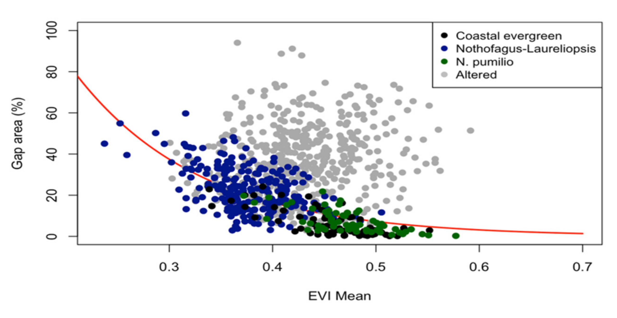
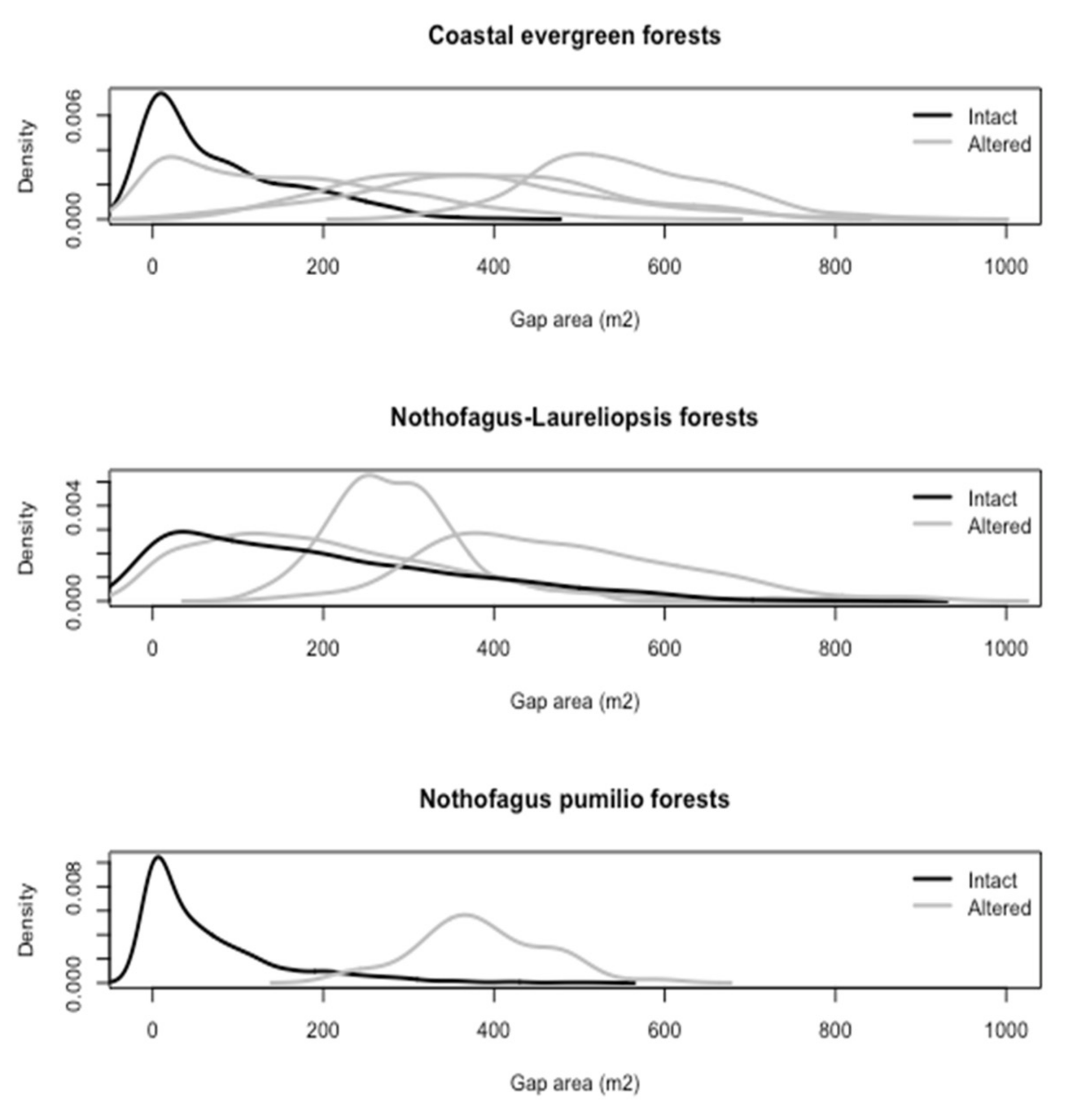
We developed a canopy alteration index using the segmentation gap metrics for each forest stand, which was calculated as follows:
IA = (%AC − utpf)/(top − utpf)
where IA is the canopy alteration index, %AC is the gap area percentage calculated using the segmentation results, utpf is the gap area percentage found in the intact forests for each forest type under analysis, and top is the gap area percentage required to consider a forest with the highest level of alteration. We also considered that IA = 0 when %AC = utpf and IA = 1 when %AC = top. The top parameter was arbitrarily set at 75% of the gap area for all forest types. We obtained the utpf parameter from the minimum value of the gap fraction along the ground-based transect from intact forests for each forest type.

3. Results

3.1. Accuracy of the Remotely Sensed Data

The percentage of the ground-detected canopy gap that we identified remotely was >60% (percentage of agreement in Table 2), in accordance with the expected trend (Spearman correlation, rho = 0.87, p < 0.001) but generally lower with respect to the values obtained in the ground-based sampling. In fact, Coastal evergreen forests presented the lowest agreement between the ground-based and segmentation data, probably due to the lesser number of gaps and their smaller size compared to the other forest stands (Table 2). The Kolmogorov–Smirnov test for gap area distributions in intact forests showed no significant or marginal differences between the ground-based and segmented data (p ranging from 0.037 to 0.5, where p < 0.05 indicates significant differences).

3.2. Comparison of Altered vs. Intact Forests

Intact forests had the lowest values in the percentage of gap area, but these values differed between the forest types (Table 2). We found that intact Coastal evergreen forests had the lowest gap area values (9%), whereas the intact Nothofagus-Laureliopsis forest type had the highest gap area values (29%). All intact forests had gap area density distributions following a log-normal distribution, but their mean and standard deviation varied among forest types (Figure 2). In accordance with their log-normal distributions, small gaps were more common (<100 m2) than large gaps (400–900 m2) in all intact forests. We did not detect any gap >900 m2 in intact forests (Figure 2). The basal area and tree density differed in the altered compared to intact forests of the same forest type (Table 2). The frequency distributions varied between the intact and altered forests of the same forest type, with evident changes in the median of the distributions as well as in the density and dispersion of the gap areas (Figure 2). For example, in stands of the Coastal evergreen forest-type, the mean gap areas increased from 79 m2 in the intact forest to 366 m2 in the altered forest. We observed that as the forests had higher mean gap areas, their gap area frequency distribution tended towards a Gaussian type distribution (Figure 2). Chusquea bamboos were present in 55% of the gaps in the intact forests and covered <70% of their area. All canopy gaps were important places for regeneration in intact forests, with saplings present in >60% of the gaps. The exception was the N. pumilio forest, where 25% of the gaps had saplings due to the high cover provided by Gaultheria sp. shrubs.
We found a strong relationship between the mean EVI values obtained from the Landsat sensor and the gap area for intact forests, but this relationship was lost for altered forests (gap area = 443.329 × exp (EVI * −8.235955), r-Spearman = −0.74, p < 0.001, Figure 3). For example, the N. pumilio and Coastal evergreen forests had mean EVI values > 0.4 with relatively small gap areas, whereas the Nothofagus-Laureliopsis forests had a mean EVI < 0.4 with larger gap areas. Both gap area and mean EVI were related to the degree of alteration of the forest stands (Table 3), but the explanatory power of the gap area was stronger than that of the mean EVI. In fact, the explanatory power of these relationships increased when the stands were analyzed by forest type (Table 3), with the Nothofagus-Laureliopsis forest-type having a stronger effect on the gap area than other forest types.

4. Discussion

Our results expanded the current knowledge on the forest canopy gap structure of temperate rainforests in the Valdivian ecoregion and revealed that intact forests (1) have distinctive canopy gap structure characteristics that are distinguishable from those of logged forests and (2) their canopy gap structure can be identified using remote sensors. Below, we discuss (1) the importance of the canopy gap structure of intact forests, (2) how our approach can be expanded to map the intact forest cover in this region, and (3) how the canopy gap structure can complement the analysis of forest degradation in this region.

4.1. Canopy Structure of Intact Forests and Their Alterations by Logging

Our results on gap area distributions in intact forests were similar to those described in other studies [53,54], which show that old-growth forests have a high frequency of small canopy gaps produced by individual treefalls. We propose that log-normal gap area distribution (Figure 2) is a distinct characteristic of intact forests in the Valdivian ecoregion since we did not find such a distribution in any of the altered forest stands. Additionally, we found that intact forests in the Valdivian ecoregion had gap areas <900 m2 (Figure 2), which is consistent with mature forests elsewhere, such as the North American temperate rain forests [55]. We found that the intact Coastal evergreen forests had a smaller gap-fraction and mean gap area compared to previously reported values for temperate rainforests (Table 3). This result reflects the capability of the very high spatial-resolution remote sensing data and the image segmentation method to explore large, forested areas, even when different remote sensing data sets are combined. In spite of using these two different kinds of remote sensing data, our study shows that the intact canopy gap structure differs among forest types in our study region (Table 3). The gap characteristics for the Nothofagus forests fell within the range reported in previous studies (Table 2 and Table 4). Other gap metrics obtained in our study were also comparable with data reported for other forests, although larger gap areas have been found in southern temperate forests (Table 4). Based on our results (Figure 2), we propose that treefall gaps with areas >900 m2 are very uncommon in intact forests of the Valdivian ecoregion. Altogether, our results on the canopy gap structure of intact forests can be used to complement the evaluation of structural characteristics found in old-growth forests in this region [10,56].
Our results support the hypothesis that the forest gap fraction, gap area frequency distribution, and mean gap area are variables that can be used to distinguish intact from altered forests in the Valdivian ecoregion. Managers and researchers could, therefore, use these variables to easily detect and measure structural changes in the canopy of altered forests via low-cost technology such as UAV images. The alteration index presented here could facilitate the classification of forests in this region according to their degree of canopy alteration and is applicable to forest types adjacent to our study area. Future research could also explore the effectiveness of this approach for other highly endangered forests in south-central Chile, such as the Mediterranean-type broadleaved Nothofagus forests.

4.2. Identifying and Mapping Intact Forests in the Valdivian Ecoregion

Previous studies have estimated deforestation and land-use change rates in the Valdivian ecoregion [60]. However, mapping intact, old-growth forests in this region remains a challenge because of their high forest structural heterogeneity [10] and topographic complexity [38]. Further, mapping intact forests requires the detection of small spatial-scale logging (e.g., removing just one tree) that is continuously degrading forests in this region. The structural attributes of the canopy in intact forests identified herein (e.g., Figure 2) provided a baseline to map intact forests in the Valdivian ecoregion, which presumably cover >500,000 ha on the Chiloé Island and the Chilean coastal range [22]. Additionally, the canopy gap structure described here can inform restoration programs of highly degraded forests and management strategies aimed at uneven-aged forest structures.
In this study, we demonstrated that, as expected, gaps > 200 m2 were more common in altered forests due to logging and can be perceived using either UAV or VHSR-SI (Figure 1 and Figure 2). In addition to patterns found in gap area frequency distributions (Figure 2), we showed that variations in a spectral vegetation index (EVI) derived from coarser spatial resolution satellite images of altered forests are related to gap areas of intact forests (Figure 3, Table 3). The EVI gap area relationship for intact forests could be influenced by the small size of treefall gaps, with a greater influence of shadows reducing the EVI value (Figure 1a). This relationship holds for intact forests of different forest types, although EVI mean and gap area values vary according to forest types (Table 3). However, the EVI mean did not change significantly for altered forests due to their higher gap area, and possibly due to the cover of Chusquea bamboos and other shrubs in the gaps (e.g., Figure 1b). Therefore, the relationship between mean EVI and gap area should be used with caution to distinguish altered from intact forests.
We propose that remote sensing data with fine spatial resolution can be used as an efficient and low-cost method to detect and monitor intact forests in the Valdivian ecoregion. Our field validation results (e.g., accuracy in Table 2) support the use of the available remote sensing datasets to quantify forest gaps in Chilean forests, where few studies exist, assessing canopy structure. We did not attempt to validate with other indirect approaches such as Digital Surface Models (DSM) from UAV images because some of our studied stands were not flown by UAV images. It would have been ideal to use only one type of data (VHSR-SI or UAV). Nevertheless, VHSR-SI was not available for all our forest stands. Moreover, many of the forest stands were inaccessible and/or presented harsh weather conditions during our fieldwork that did not allow us to use a UAV system. Considering these limitations, future research could explore the use of DSM from UAV images to identify canopy gaps. Such an analysis could potentially expand the validation of our results. In addition, future research could focus on the spatially upscaling of these results and explore EVI trajectories, which can be related to spatiotemporal changes in biomass [61,62,63]. LiDAR data, spectral mixture analysis, texture analyses of images, and machine learning techniques can enhance or complement this approach to produce maps of forest degradation [64,65,66,67,68,69]. In addition to the application presented here, these techniques could also be used to estimate variables such as the height of the upper canopy, height profiles of forests, and the estimation of aboveground biomass, among other applications [69]. However, for many forests in the world, LiDAR is not available, or UAV flights are difficult to implement due to accessibility. In those cases, VHSR-SI is the only choice. The constellation of such satellites has been growing, providing worldwide coverage with a higher temporal resolution (e.g., the Pleiades constellation). Implementing VHSR-SI to monitor forest degradation would generate significant savings in economic and human resources, both of which are in short supply in countries such as Chile and Argentina.

4.3. Detecting Logging and Complementing Forest Degradation Criteria

Our method to detect intact, old-growth forests could be extended, as discussed above, to detect illegal logging. In Chile, approximately 90% of logging activities are illegal, causing degradation in native forests of high diversity and high carbon density [24,70]. Despite its pervasiveness, we lack both yearly and regional quantitative data on illegal logging in Chile. As shown in our research, the monitoring of intact forests through remote sensing data with fine spatial resolution has a high potential for photogrammetry since it is possible to map the horizontal and vertical structure of the forest and identify treefall gaps in detail (e.g., Figure 1c,d). This approach is a cost-effective tool both to quantify illegal logging and to supervise forest management plans focused on sustainable, selective loggings in uneven-aged forests (e.g., producing small canopy gaps). One of the main advantages of using either VHSR-SI or UAV images is their potential to reduce the sampling time in degraded forests that are hard to access and transit. Using the methods proposed in this research, managers can make high-precision measurements based on images obtained from UAVs. Furthermore, as forest canopy gaps play a fundamental role in the potential recovery of the structure of an altered forest [71], the analysis of the canopy gap structure using remote sensing data with fine spatial resolution can assist in decision-making processes to evaluate the best silvicultural strategies for forest recovery.
Forest degradation is a process that derives from the anthropic alteration of ecosystems and generates a loss of productivity, biodiversity, and structure [72]. Degradation implies the alteration or persistent change of ecosystem attributes due to direct or indirect human activities such as logging, fires, introduction of exotic species, land-use changes, etc. [72,73]. Since these processes act synergistically, managers need to address them in combination. Thus, identifying changes in the canopy gap structure should be complemented with other criteria for assessing forest degradation in the Valdivian ecoregion.

5. Conclusions

Intact forests in the Valdivian ecoregion have a distinguishable canopy gap structure that can be used to develop criteria for their detection. The alterations of the canopy of intact forests due to logging in this region are associated with the distribution of the canopy gap area and are detectable using very high spatial resolution images. These results are steps forward in the refinement of criteria to evaluate the state of alteration of forests. Such an effort will help curtail the loss of unique biodiversity, changes in biogeochemical cycles, and carbon emissions to the atmosphere in a region which still has extensive, intact forest landscapes. The approach developed in this study is a fast, low-cost, and reliable method to obtain canopy structure indicators that are useful for identifying intact forest canopies and for managers interested in maintaining and restoring uneven-aged forests in southern temperate rainforests.

Author Contributions

Conceptualization, writing—original draft preparation, and funding acquisition Á.G.G.; methodology, all authors; I.D.-H. formal analysis; writing—review and editing, all authors. All authors have read and agreed to the published version of the manuscript.

Funding

This work was supported by Fondo de Investigación Bosque Nativo [grant number 27/2015] and Programa de Estímulo a la Excelencia Institucional 2017 Universidad de Chile [PEEI.2017].

Data Availability Statement

The data presented in this study are available on request from the corresponding author.

Acknowledgments

We acknowledge the landowners and CONAF that allowed us to work in their forests. We thank E. Arias, T. Matamala, A. Lara, A. Oyarzún, D. Nuñez, J. Poblete, R. Novoa, Y. Asenie for the field assistance. We thank the editors and anonymous reviewers that provided useful comments.

Conflicts of Interest

The authors declare no conflict of interest.

References

  1. Mackey, B.; DellaSala, D.A.; Kormos, C.; Lindenmayer, D.; Kumpel, N.; Zimmerman, B.; Hugh, S.; Young, V.; Foley, S.; Arsenis, K.; et al. Policy Options for the World’s Primary Forests in Multilateral Environmental Agreements. Conserv. Lett. 2015, 8, 139–147. [Google Scholar] [CrossRef] [Green Version]
  2. Potapov, P.; Hansen, M.C.; Laestadius, L.; Turubanova, S.; Yaroshenko, A.; Thies, C.; Smith, W.; Zhuravleva, I.; Komarova, A.; Minnemeyer, S.; et al. The Last Frontiers of Wilderness: Tracking Loss of Intact Forest Landscapes from 2000 to 2013. Sci. Adv. 2017, 3, e1600821. [Google Scholar] [CrossRef] [PubMed] [Green Version]
  3. Hansen, M.C.; Potapov, P.V.; Moore, R.; Hancher, M.; Turubanova, S.A.; Tyukavina, A.; Thau, D.; Stehman, S.V.; Goetz, S.J.; Loveland, T.R.; et al. High-Resolution Global Maps of 21st-Century Forest Cover Change. Science 2013, 342, 850–853. [Google Scholar] [CrossRef] [PubMed] [Green Version]
  4. Kim, D.-H.; Sexton, J.O.; Townshend, J.R. Accelerated Deforestation in the Humid Tropics from the 1990s to the 2000s. Geophys. Res. Lett. 2015, 42, 3495–3501. [Google Scholar] [CrossRef] [PubMed]
  5. Laurance, W.F.; Nascimento, H.E.M.; Laurance, S.G.; Andrade, A.C.; Fearnside, P.M.; Ribeiro, J.E.L.; Capretz, R.L. Rain Forest Fragmentation and the Proliferation of Successional Trees. Ecology 2006, 87, 469–482. [Google Scholar] [CrossRef]
  6. Watson, J.E.M.; Evans, T.; Venter, O.; Williams, B.; Tulloch, A.; Stewart, C.; Thompson, I.; Ray, J.C.; Murray, K.; Salazar, A.; et al. The Exceptional Value of Intact Forest Ecosystems. Nat. Ecol. Evol. 2018, 2, 599–610. [Google Scholar] [CrossRef] [PubMed]
  7. Edenhofer, O.; Pichs-Madruga, R.; Sokona, Y.; Farahani, E.; Kadner, S.; Seyboth, K.; Adler, A.; Baum, I.; Brunner, S.; Eickemeier, P.; et al. IPCC, 2014: Climate Change 2014: Mitigation of Climate Change. Contribution of Working Group III to the Fifth Assessment Report of the Intergovernmental Panel on Climate Change; Cambridge University Press: Cambridge, UK, 2014. [Google Scholar]
  8. Smith, J.B.; Schneider, S.H.; Oppenheimer, M.; Yohe, G.W.; Hare, W.; Mastrandrea, M.D.; Patwardhan, A.; Burton, I.; Corfee-Morlot, J.; Magadza, C.H.D.; et al. Assessing Dangerous Climate Change through an Update of the Intergovernmental Panel on Climate Change (IPCC) “Reasons for Concern” . Proc. Natl. Acad. Sci. USA 2009, 106, 4133–4137. [Google Scholar] [CrossRef] [PubMed] [Green Version]
  9. Armesto, J.J.; Smith-Ramírez, C.; Carmona, M.R.; Celis-Diez, J.L.; Díaz, I.A.; Gaxiola, A.; Gutiérrez, A.G.; Núñez-Avila, M.C.; Pérez, C.A.; Rozzi, R. Old-Growth Temperate Rainforests of South America: Conservation, Plant–Animal Interactions, and Baseline Biogeochemical Processes. In Old-Growth Forests; Ecological Studies; Wirth, C., Gleixner, G., Heimann, M., Eds.; Springer: Berlin/Heidelberg, Germany, 2009; pp. 367–390. ISBN 978-3-540-92705-1. [Google Scholar]
  10. Gutiérrez, A.G.; Armesto, J.J.; Aravena, J.-C.; Carmona, M.; Carrasco, N.V.; Christie, D.A.; Peña, M.-P.; Pérez, C.; Huth, A. Structural and Environmental Characterization of Old-Growth Temperate Rainforests of Northern Chiloé Island, Chile: Regional and Global Relevance. For. Ecol. Manag. 2009, 258, 376–388. [Google Scholar] [CrossRef]
  11. Hendrickson, O. Old-Growth Forests: Data Gaps and Challenges. For. Chron. 2003, 79–3, 645–651. [Google Scholar] [CrossRef] [Green Version]
  12. Foster, D.R.; Orwlg, D.A.; McLachlan, J.S. Ecological and Conservation Insights from Reconstructive Studies of Temperate Old-Growth Forests. Trends Ecol. Evol. 1996, 11, 419–424. [Google Scholar] [CrossRef]
  13. Franklin, J.F.; Spies, T.A.; Pelt, R.V.; Carey, A.B.; Thornburgh, D.A.; Berg, D.R.; Lindenmayer, D.B.; Harmon, M.E.; Keeton, W.S.; Shaw, D.C.; et al. Disturbances and Structural Development of Natural Forest Ecosystems with Silvicultural Implications, Using Douglas-Fir Forests as an Example. For. Ecol. Manag. 2002, 155, 399–423. [Google Scholar] [CrossRef]
  14. Franklin, J.F.; Cromack, K.J.; Denison, W.; McKee, A.; Maser, C.; Sedell, J.; Swanson, F.; Juday, G. Ecological Characteristics of Old-Growth Douglas-Fir Forests; General Technical Report (GTR); U.S. Department of Agriculture, Forest Service, Pacific Northwest Research Station: Portland, OR, USA, 1981. [CrossRef]
  15. Wirth, C.; Gleixner, G.; Heimann, M. Old-Growth Forests: Function, Fate and Value; Springer Science & Business Media: Berlin/Heidelberg, Germany, 2009; ISBN 978-3-540-92706-8. [Google Scholar]
  16. Runkle, J.R. Gap Regeneration in Some Old-Growth Forests of the Eastern United States. Ecology 1981, 62, 1041–1051. [Google Scholar] [CrossRef]
  17. De Sy, V.; Herold, M.; Achard, F.; Asner, G.P.; Held, A.; Kellndorfer, J.; Verbesselt, J. Synergies of Multiple Remote Sensing Data Sources for REDD+ Monitoring. Curr. Opin. Environ. Sustain. 2012, 4, 696–706. [Google Scholar] [CrossRef]
  18. Baumann, M.; Ozdogan, M.; Wolter, P.T.; Krylov, A.; Vladimirova, N.; Radeloff, V.C. Landsat Remote Sensing of Forest Windfall Disturbance. Remote Sens. Environ. 2014, 143, 171–179. [Google Scholar] [CrossRef]
  19. Chambers, J.Q.; Negron-Juarez, R.I.; Marra, D.M.; Vittorio, A.D.; Tews, J.; Roberts, D.; Ribeiro, G.H.P.M.; Trumbore, S.E.; Higuchi, N. The Steady-State Mosaic of Disturbance and Succession across an Old-Growth Central Amazon Forest Landscape. Proc. Natl. Acad. Sci. USA 2013, 110, 3949–3954. [Google Scholar] [CrossRef] [Green Version]
  20. Espírito-Santo, F.D.B.; Gloor, M.; Keller, M.; Malhi, Y.; Saatchi, S.; Nelson, B.; Junior, R.C.O.; Pereira, C.; Lloyd, J.; Frolking, S.; et al. Size and Frequency of Natural Forest Disturbances and the Amazon Forest Carbon Balance. Nat. Commun. 2014, 5. [Google Scholar] [CrossRef] [PubMed] [Green Version]
  21. Chambers, J.Q.; Asner, G.P.; Morton, D.C.; Anderson, L.O.; Saatchi, S.S.; Espírito-Santo, F.D.B.; Palace, M.; Souza, C. Regional Ecosystem Structure and Function: Ecological Insights from Remote Sensing of Tropical Forests. Trends Ecol. Evol. 2007, 22, 414–423. [Google Scholar] [CrossRef]
  22. Smith-Ramírez, C. The Chilean Coastal Range: A Vanishing Center of Biodiversity and Endemism in South American Temperate Rainforests. Biodivers. Conserv. 2004, 13, 373–393. [Google Scholar] [CrossRef]
  23. Armesto, J.J.; Rozzi, R.; Smith-Ramírez, C.; Arroyo, M.T.K. Conservation Targets in South American Temperate Forests. Science 1998, 282, 1271–1272. [Google Scholar] [CrossRef] [Green Version]
  24. Armesto, J.J.; Manuschevich, D.; Mora, A.; Smith-Ramirez, C.; Rozzi, R.; Abarzúa, A.M.; Marquet, P.A. From the Holocene to the Anthropocene: A Historical Framework for Land Cover Change in Southwestern South America in the Past 15,000 Years. Land Use Policy 2010, 27, 148–160. [Google Scholar] [CrossRef]
  25. Lara, A.; Soto, D.; Armesto, J.; Donoso, P.; Wernli, C.; Nahuelhual, L.; Squeo, F. (Eds.) Componentes Científicos Clave Para Una Política Nacional Sobre Usos, Servicios y Conservación de Los Bosques Nativos Chilenos; Universidad Austral de Chile, Iniciativa Científica Milenio de MIDEPLAN: Valdivia, Chile, 2003; ISBN 956-299-005-2. [Google Scholar]
  26. Heilmayr, R.; Echeverría, C.; Lambin, E.F. Impacts of Chilean Forest Subsidies on Forest Cover, Carbon and Biodiversity. Nat. Sustain. 2020, 3, 701–709. [Google Scholar] [CrossRef]
  27. Gutierrez, A.G. Long-Term Dynamics and the Response of Temperate Rainforests of Chiloé Island (Chile) to Climate Change. Ph.D. Thesis, Technische Universität München, Munich, Germany, 2010. [Google Scholar]
  28. Keith, H.; Mackey, B.G.; Lindenmayer, D.B. Re-Evaluation of Forest Biomass Carbon Stocks and Lessons from the World’s Most Carbon-Dense Forests. Proc. Natl. Acad. Sci. USA 2009, 106, 11635–11640. [Google Scholar] [CrossRef] [Green Version]
  29. Perez-Quezada, J.F.; Olguín, S.; Fuentes, J.P.; Galleguillos, M. Reservorio de Carbono Arbóreo En Bosques Siempreverdes de Chiloé, Chile. Bosque Valdivia 2015, 36, 27–39. [Google Scholar] [CrossRef] [Green Version]
  30. Urrutia-Jalabert, R.; Malhi, Y.; Lara, A. The Oldest, Slowest Rainforests in the World? Massive Biomass and Slow Carbon Dynamics of Fitzroya Cupressoides Temperate Forests in Southern Chile. PLoS ONE 2015, 10, e0137569. [Google Scholar] [CrossRef] [PubMed] [Green Version]
  31. Lara, A.; Solari, M.E.; del Rosario Prieto, M.; Peña, M.P. Reconstruction of vegetation cover and land use ca. 1550 and their change towards 2007 in the Valdivian Rainforest Ecoregion of Chile (35°–43°30′ S). Bosque 2012, 33, 13–23. [Google Scholar] [CrossRef] [Green Version]
  32. Schlegel, B.C.; Donoso, P.J. Effects of Forest Type and Stand Structure on Coarse Woody Debris in Old-Growth Rainforests in the Valdivian Andes, South-Central Chile. For. Ecol. Manag. 2008, 255, 1906–1914. [Google Scholar] [CrossRef]
  33. Ponce, D.B.; Donoso, P.J.; Salas-Eljatib, C.; Ponce, D.B.; Donoso, P.J.; Salas-Eljatib, C. Índice de Bosque Adulto: Una Herramienta Para Evaluar Estados de Desarrollo de Bosques Nativos de Tierras Bajas Del Centro-Sur de Chile. Bosque Valdivia 2019, 40, 235–240. [Google Scholar] [CrossRef] [Green Version]
  34. Oyarzún, A.; Donoso, P.J.; Gutiérrez, Á.G. Patrones de Distribución de Alturas de Bosques Antiguos Siempreverde Del Centro-Sur de Chile. Bosque Valdivia 2019, 40, 355–364. [Google Scholar] [CrossRef] [Green Version]
  35. Alaback, P.B. Comparative Ecology of Temperate Rainforests of the Americas along Analogous Climatic Gradients. Rev. Chil. Hist. Nat. 1991, 64, 399–412. [Google Scholar]
  36. Veblen, T.T.; Schlegel, F.M.; Oltremari, J.V. Temperate broad-leaved evergreen forests of South America. In Temperate Broad-Leaved Evergreen Forests; Elsevier: Amsterdam, The Netherlands, 1983; pp. 5–31. [Google Scholar]
  37. Arroyo, M.T.K.; Riveros, M.; Peñaloza, A.; Cavieres, L.; Faggi, A.M. Phytogeographic Relationships and Regional Richness Patterns of the Cool Temperate Rainforest Flora of Southern South America. In High-Latitude Rainforests and Associated Ecosystems of the West Coast of the Americas; Lawford, R.G., Fuentes, E., Alaback, P.B., Eds.; Springer: New York, NY, USA, 1996; pp. 134–172. ISBN 978-1-4612-8453-6. [Google Scholar]
  38. Donoso, C. Bosques Templados de Chile y Argentina: Variación, Estructura y Dinámica; Editorial Universitaria: Santiago, Chile, 1993; ISBN 978-956-11-0926-1. [Google Scholar]
  39. CONAF. Catastro de Los Recursos Vegetacionales Nativos de Chile. Monitoreo de Cambios y Actualizaciones Periodo 1997–2011; Corporación Nacional Forestal: Santiago, Chile, 2011; p. 28. [Google Scholar]
  40. Gutiérrez, A.G.; Huth, A. Successional Stages of Primary Temperate Rainforests of Chiloé Island, Chile. Perspect. Plant. Ecol. Evol. Syst. 2012, 14, 243–256. [Google Scholar] [CrossRef]
  41. Runkle, J.R. Patterns of Disturbance in Some Old-Growth Mesic Forests of Eastern North America. Ecology 1982, 63, 1533–1546. [Google Scholar] [CrossRef] [Green Version]
  42. Runkle, J.R. Guidelines and Sample Protocol for Sampling Forest Gaps; U.S. Department of Agriculture, Forest Service, Pacific Northwest Research Station: Portland, OR, USA, 1992.
  43. Kuester, M. Absolute Radiometric Calibration: 2015v2; Digital Globe: Longmont, CO, USA, 2016. [Google Scholar]
  44. Comaniciu, D.; Meer, P. Mean Shift: A Robust Approach toward Feature Space Analysis. IEEE Trans. Pattern Anal. Mach. Intell. 2002, 24, 603–619. [Google Scholar] [CrossRef] [Green Version]
  45. Dallal, G.E.; Wilkinson, L. An Analytic Approximation to the Distribution of Lilliefors’s Test Statistic for Normality. Am. Stat. 1986, 40, 294–296. [Google Scholar] [CrossRef]
  46. Royston, J.P. An Extension of Shapiro and Wilk’s W Test for Normality to Large Samples. J. R. Stat. Soc. Ser. C Appl. Stat. 1982, 31, 115–124. [Google Scholar] [CrossRef]
  47. Venables, W.N.; Ripley, B.D. Modern Applied Statistics with S, 4th ed.; Statistics and Computing; Springer: New York, NY, USA, 2002; ISBN 978-0-387-95457-8. [Google Scholar]
  48. Bates, D.M.; Watts, D.G. Nonlinear Regression Analysis and Its Applications; Wiley Series in Probability and Statistics; John and Wiley and Sons: Hoboken, NJ, USA, 1988; ISBN 978-0-471-81643-0. [Google Scholar]
  49. Menard, S. Applied Logistic Regression Analysis; SAGE Publications: Thousand Oaks, CA, USA, 2001; ISBN 978-1-5443-3258-1. [Google Scholar]
  50. Kumar, R.; Nandy, S.; Agarwal, R.; Kushwaha, S.P.S. Forest Cover Dynamics Analysis and Prediction Modeling Using Logistic Regression Model. Ecol. Indic. 2014, 45, 444–455. [Google Scholar] [CrossRef]
  51. Hosmer, D.W.; Hosmer, T.; Cessie, S.L.; Lemeshow, S. A Comparison of Goodness-of-Fit Tests for the Logistic Regression Model. Stat. Med. 1997, 16, 965–980. [Google Scholar] [CrossRef]
  52. R Core Team. R: A Language and Environment for Statistical Computing; R Foundation for Statistical Computing: Vienna, Austria, 2019. [Google Scholar]
  53. Bartemucci, P.; Coates, K.D.; Harper, K.A.; Wright, E.F. Gap Disturbances in Northern Old-Growth Forests of British Columbia, Canada. J. Veg. Sci. 2002, 13, 685–696. [Google Scholar] [CrossRef]
  54. McCarthy, J. Gap Dynamics of Forest Trees: A Review with Particular Attention to Boreal Forests. Environ. Rev. 2001, 9, 1–59. [Google Scholar] [CrossRef]
  55. Lertzman, K.P.; Sutherland, G.D.; Inselberg, A.; Saunders, S.C. Canopy Gaps and the Landscape Mosaic in a Coastal Temperate Rain Forest. Ecology 1996, 77, 1254–1270. [Google Scholar] [CrossRef]
  56. Ponce, D.B.; Donoso, P.J.; Salas-Eljatib, C. Differentiating Structural and Compositional Attributes across Successional Stages in Chilean Temperate Rainforests. Forests 2017, 8, 329. [Google Scholar] [CrossRef] [Green Version]
  57. Gutiérrez, A.G.; Aravena, J.C.; Carrasco-Farías, N.V.; Christie, D.A.; Fuentes, M.; Armesto, J.J. Gap-Phase Dynamics and Coexistence of a Long-Lived Pioneer and Shade-Tolerant Tree Species in the Canopy of an Old-Growth Coastal Temperate Rain Forest of Chiloé Island, Chile. J. Biogeogr. 2008, 35, 1674–1687. [Google Scholar] [CrossRef]
  58. Nagel, T.A.; Svoboda, M.; Kobal, M. Disturbance, Life History Traits, and Dynamics in an Old-Growth Forest Landscape of Southeastern Europe. Ecol. Appl. 2014, 24, 663–679. [Google Scholar] [CrossRef]
  59. Promis, A. Claros de dosel en bosques nativos templados de Chile y Argentina: Conocimientos actuales y desafíos para el futuro. In Silvicultura en Bosques Nativos; Chile Initiative, OSU College of Forestry: Corvallis, OR, USA, 2018; pp. 23–50. [Google Scholar]
  60. Miranda, A.; Altamirano, A.; Cayuela, L.; Lara, A.; González, M. Native Forest Loss in the Chilean Biodiversity Hotspot: Revealing the Evidence. Reg. Environ. Change 2017, 17, 285–297. [Google Scholar] [CrossRef]
  61. Huete, A.; Didan, K.; Miura, T.; Rodriguez, E.P.; Gao, X.; Ferreira, L.G. Overview of the Radiometric and Biophysical Performance of the MODIS Vegetation Indices. Remote Sens. Environ. 2002, 83, 195–213. [Google Scholar] [CrossRef]
  62. Shimizu, K.; Ponce-Hernandez, R.; Ahmed, O.S.; Ota, T.; Win, Z.C.; Mizoue, N.; Yoshida, S. Using Landsat Time Series Imagery to Detect Forest Disturbance in Selectively Logged Tropical Forests in Myanmar. Can. J. For. Res. 2016, 47, 289–296. [Google Scholar] [CrossRef] [Green Version]
  63. Verbesselt, J.; Hyndman, R.; Newnham, G.; Culvenor, D. Detecting Trend and Seasonal Changes in Satellite Image Time Series. Remote Sens. Environ. 2010, 114, 106–115. [Google Scholar] [CrossRef]
  64. Asner, G.P.; Keller, M.; Pereira, R., Jr.; Zweede, J.C.; Silva, J.N.M. Canopy Damage and Recovery after Selective Logging in Amazonia: Field and Satellite Studies. Ecol. Appl. 2004, 14, 280–298. [Google Scholar] [CrossRef] [Green Version]
  65. Asner, G.P.; Keller, M.; Pereira, R.; Zweede, J.C. Remote Sensing of Selective Logging in Amazonia: Assessing Limitations Based on Detailed Field Observations, Landsat ETM+, and Textural Analysis. Remote Sens. Environ. 2002, 80, 483–496. [Google Scholar] [CrossRef]
  66. Asner, G.P.; Heidebrecht, K.B. Spectral Unmixing of Vegetation, Soil and Dry Carbon Cover in Arid Regions: Comparing Multispectral and Hyperspectral Observations. Int. J. Remote Sens. 2002, 23, 3939–3958. [Google Scholar] [CrossRef]
  67. Mao, X.; Hou, J. Object-Based Forest Gaps Classification Using Airborne LiDAR Data. J. For. Res. 2019, 30, 617–627. [Google Scholar] [CrossRef]
  68. Tang, H.; Armston, J.; Hancock, S.; Marselis, S.; Goetz, S.; Dubayah, R. Characterizing Global Forest Canopy Cover Distribution Using Spaceborne Lidar. Remote Sens. Environ. 2019, 231, 111262. [Google Scholar] [CrossRef]
  69. Ota, T.; Ahmed, O.S.; Minn, S.T.; Khai, T.C.; Mizoue, N.; Yoshida, S. Estimating Selective Logging Impacts on Aboveground Biomass in Tropical Forests Using Digital Aerial Photography Obtained before and after a Logging Event from an Unmanned Aerial Vehicle. For. Ecol. Manag. 2019, 433, 162–169. [Google Scholar] [CrossRef]
  70. Bannister, J.R.; Vargas-Gaete, R.; Ovalle, J.F.; Acevedo, M.; Fuentes-Ramirez, A.; Donoso, P.J.; Promis, A.; Smith-Ramírez, C. Major Bottlenecks for the Restoration of Natural Forests in Chile. Restor. Ecol. 2018, 26, 1039–1044. [Google Scholar] [CrossRef] [Green Version]
  71. Bauhus, J.; Puettmann, K.; Messier, C. Silviculture for Old-Growth Attributes. For. Ecol. Manag. 2009, 258, 525–537. [Google Scholar] [CrossRef] [Green Version]
  72. Ghazoul, J.; Chazdon, R. Degradation and Recovery in Changing Forest Landscapes: A Multiscale Conceptual Framework. Annu. Rev. Environ. Resour. 2017, 42, 161–188. [Google Scholar] [CrossRef] [Green Version]
  73. Achard, F.; Eva, H.; Mollicone, D.; Popatov, P.; Stibig, H.-J.; Turubanova, S.; Yaroshenko, A. Detecting Intact Forests from Space: Hot Spots of Loss, Deforestation and the UNFCCC. In Old-Growth Forests; Ecological Studies; Wirth, C., Gleixner, G., Heimann, M., Eds.; Springer: Berlin/Heidelberg, Germany, 2009; pp. 411–427. ISBN 978-3-540-92705-1. [Google Scholar]
Figure 1. Example of intact forest canopies in Hueicolla (a) and San Pablo de Tregua (c) compared to altered forest canopies due to logging in Lomas del Sol (b) and Raulintal2 (d). Note how treefall gaps are small in size in (a) with a greater influence of shadows, whereas canopy gaps in the altered stand (b) are filled by Chusquea bamboos. Examples of the segmentation results are shown in (c) and (d).
Forests 12 01183 g001
Figure 2. Comparison of the gap area frequency distributions in altered and intact forests.
Forests 12 01183 g002
Figure 3. The relationship between the mean EVI calculated in the Landsat grid for each forest stand studied and the gap area percentage in each cell. Blue, black, and green dots indicate data from intact forests. The red line is the best nonlinear model adjusted to data from intact forests.
Forests 12 01183 g003
Table 1. Forest stand characteristics and remote-sensing data used in this study. UAV: unmanned aerial vehicle mosaic; VHSR-SI: very high spatial-resolution satellite imagery.
Forest Stand NameLatitudeLongitudeElevationStand Area (ha)Alteration StatusRemote Sensing Data
Coastal evergreen
Cutipay−39.84−73.363408.9AlteredUAV
Hueicolla−40.16−73.6127057.5IntactVHSR-SI
Llancahue−39.85−73.1333086.7AlteredUAV
Lomas del Sol−39.83−73.1429045.4AlteredUAV
Pilolkura−39.70−73.34480147.4AlteredVHSR-SI
Raulintal2−40.24−73.3960017.8AlteredUAV
Nothofagus—Laureliopsis
Ankacoihue−39.78−71.87101016.2AlteredUAV
Epulafquen−39.76−71.75720106.1IntactVHSR-SI
Raulintal1−40.22−73.3768025.9AlteredUAV
San Pablo de Tregua−39.60−72.0990081.8IntactVHSR-SI
Nothofagus pumilio
Choshuenco−39.94−72.1210105.7AlteredUAV
Antillanca−40.78−72.19123050.2IntactVHSR-SI
Table 2. The forest canopy gap structure of the stands studied in the Valdivian ecoregion. Accuracy refers to the percentage of ground-detected canopy gaps identified remotely using very high-resolution data.
Forest TypeSite NameCanopy-Alteration Index (-) Ground-Based DataImage-Segmentation Data
Basal Area Stand DensityForest Gap AreaNumber of GapsForest Gap AreaMean Gap AreaAccuracy
(m2/ha)(Trees/ha)(%)(Count)(%)(m2)(%)
Coastal evergreen
Hueicolla088.23127910279.260
Llancahue0.0868.9100932.52115156.988
Lomas del Sol0.3240.8139343273036658
Cutipay0.5133302042.33143385.975
Pilolkura0.66no datano data63.43052368.473.3
Raulintal20.85no datano data66.43965554.463
Nothofagus—Laureliopsis
San Pablo de Tregua0142.487828.82124194.678
Epulafquen0.13148.172031.31935200.884
Ankacoihue0.5150.8111168.23952291.694.9
Raulintal10.57no datano data66.43965554.4100
Nothofagus pumilio
Antillanca055.6248011.820364.970
Choshuenco0.22no datano data30.83139384.190.3
Table 3. Univariate and multiple logistic regression models that explain the variation of the total gap area and mean EVI with the degree of alteration (intact/altered) and forest type. AIC: Akaike information criterion. See also the Materials and Methods Section for an explanation of the statistical analysis. * indicates p < 0.01, *** indicates p < 0.001.
Explanatory Variables
Gap AreaMean EVI
Univariate models
Regression coefficientsEstimatePr(>|z|) EstimatePr(>|z|)
Intercept−2.19<2 × 10⁻¹⁶***−3.07379.62 × 10−8***
Slope1.14 × 10−3<2 × 10⁻¹⁶***7.75441.37 × 10−8***
Model statistics
AIC811.0 1075.1
Goodness of fit 298.4 34.20
Model chi-square 7.51 × 10−67 4.97 × 10⁻⁹
Pseudo r20.27 0.03
Multiple models
Regression coefficients
Intercept−1.8514.06 × 10−11***0.41070.6204
Variable0.003<2 × 10⁻¹⁶***4.86650.0118*
Nothofagus-Laureliopsis −7.243<2 × 10⁻¹⁶***−3.0086<2 × 10⁻¹⁶***
Nothofagus pumilio−8.3290.064 −4.0522<2 × 10⁻¹⁶***
Coastal evergreen-- --
Model statistics
AIC307.2 709.3
Goodness of fit 806.2 404.0
Model chi-square 2.00 × 10−174 2.99 × 10−87
Pseudo r20.73 0.37
Table 4. Gap characteristics found in the forests of the world. Data obtained from [53,54,55,57,58,59].
Forest TypeGap FractionMean Gap AreaMaximum Gap Area
(Range %)(Range m2)(Range m2)
Northern Hemisphere
Boreal and subalpine6–7725–17612–1245
Temperate hardwood 2–2028–400144–2009
Temperate coniferous 14–4619–131380–734
Tropical forests0.8–810–120135–700
Southern Hemisphere
New Zealand subalpine montane2.540–68
South American temperate
rainforest
3.3–8.6151–4321532
South American old-growth Nothofagus temperate rainforests4–3561–8983462
South American old-growth
Fitzroya temperate rainforests
143736
South African plateau2–1020–38122
Publisher’s Note: MDPI stays neutral with regard to jurisdictional claims in published maps and institutional affiliations.

