Growing Stock Volume Retrieval from Single and Multi-Frequency Radar Backscatter

Abstract

While products generated at global levels provide easy access to information on forest growing stock volume (GSV), their use at regional to national levels is limited by temporal frequency, spatial resolution, or unknown local errors that may be overcome through locally calibrated products. This study assessed the need, and utility, of developing locally calibrated GSV products for the Romanian forests. To this end, we used national forest inventory (NFI) permanent sampling plots with largely concurrent SAR datasets acquired at C- and L-bands to train and validate a machine learning algorithm. Different configurations of independent variables were evaluated to assess potential synergies between C- and L-band. The results show that GSV estimation errors at C- and L-band were rather similar, relative root mean squared errors (RelRMSE) around 55% for forests averaging over 450 m³ ha⁻¹, while synergies between the two wavelengths were limited. Locally calibrated models improved GSV estimation by 14% when compared to values obtained from global datasets. However, even the locally calibrated models showed particularly large errors over low GSV intervals. Aggregating the results over larger areas considerably reduced (down to 25%) the relative estimation errors.

1. Introduction

Forests are among the most biodiverse terrestrial ecosystems and a key element for carbon sequestration as they store large amounts of organic matter (i.e., biomass). Therefore, forest above ground biomass (AGB) estimation is a sensitive research topic, as information on AGB levels and dynamics is needed to estimate greenhouse gases flux and thus to shape policies development, implementation, and monitoring [1]. This importance is highlighted by the countless forest inventory programs aimed at evaluating, monitoring, and reporting, among others, AGB or Growing Stock Volume (GSV) levels. Such programs use an array of data sources from in situ measurements to information acquired by earth observation (EO) platforms. In situ surveys, based on systematic sampling grids, are the backbone of traditional national forest inventory (NFI) programs sometimes stretching back centuries [2]. However, NFI programs are expensive and time consuming while not providing for a synoptic view across the landscape [3].

With the development of EO technologies, new avenues were open as the systematic data collection allowed for frequent, spatially resolved AGB or GSV estimates to be derived within a range of national and global initiatives, such as the Japan Aerospace Exploration Agency (JAXA) Kyoto and Carbon (KC) Initiative, the United Nation Collaborative Programme on Reducing Emissions from Deforestation and Forest Degradation (REDD), NASA’s Carbon Monitoring System (CMS), and the European Space Agency (ESA) Climate Change Initiative (CCI). Forest AGB was estimated from optical, radar, and lidar sensors. Tracking forest properties with optical sensors is usually limited to the first decades of development [4]. Lidar sensors provide very accurate information on forest vertical structure [5], but their use is limited by temporal (airborne) or spatial (space borne) coverage and cloud presence. As the radar signal is directly influenced by the vegetation structure, synthetic aperture radar (SAR) sensors are more sensitive to AGB levels when compared to optical data, and less limited by spatial and temporal availability when compared to Lidar data [6]. Therefore, over the past two decades SAR sensors have been widely used to retrieve forest biomass at a regional to global level due to constant improvements in coverage and temporal and spatial resolutions, as well as independence from cloud cover [7,8,9,10,11,12,13]. Such studies used a variety of modelling approaches, including empirical, semi-empirical, numerical, and non-parametric modelling. Regardless of the models used, the major limitation of spaceborne SAR observations is the sensitivity to forest unrelated variables which result in substantial uncertainties and AGB-dependent biases [14].

From the first prototype studies in the 1990s which evaluated the capability of a certain set of optical and SAR observations to estimate GSV or AGB, recent studies in the 2000s demonstrated that a combination of observations is beneficial to map biomass across extended landscapes. While most studies reported on estimating biomass at local to regional scale, a range of projects targeted biomass mapping at continental to a global scale [13,15,16,17,18,19,20]. However, such data products are of limited use at national level due to the (i) limited sensitivity to biomass, obtained through indirect relationship requiring inference with models and approximations, (ii) low temporal frequency (e.g., one off), (iii) generally low (>100 m) spatial resolution, (iv) unknown errors at national levels, (v) compromises in the retrieval algorithms which need to account for a wide range of conditions (e.g., boreal to tropical), and (v) the lack of calibration data over large tracts of forests with the in situ data used for algorithm development being sourced from relatively few countries. Such limitations translate into discrepancies between in situ and mapped biomass stocks. Indeed, many studies have shown differences between the global products specified accuracy and in situ samples over national to regional scales [14,18,21,22,23,24] with locally calibrated products providing significant improvements for the estimated forest parameters [14,23,24,25].

Forests are under constant pressure due to anthropogenic factors related to clearing activities and changes in land use with approximately 4.5% of the Romanian forests being affected by at least one disturbance event (complete or nearly complete tree removal) over the past two decades. The high rate of forest disturbance, as estimated from remote sensing datasets [26], suggest changes in Romanian forests growing stock volume as significant as those caused by climate changes alone [27,28]. However, spatially explicit GSV estimates are not available for the Romanian forests, as remote sensing technologies were mostly used to estimate forest cover rather than GSV [26,29,30]. The hypothesis of this study was that SAR datasets may provide the means to derive spatially explicit estimates of GSV with higher frequency when compared to the five-year cycle of the National Forest Inventory (NFI) and lower errors when compared to globally derived GSV estimates [13,20]. The aim of this study was to ascertain the utility of locally calibrated models, based on in situ NFI information and SAR datasets, for GSV estimation in the Romanian forests. The specific objectives were to (i) calibrate single- and multi-frequency SAR-based models for GSV retrieval in the Romanian forests, and (ii) ascertain the synergies of C- and L-band SAR datasets for GSV retrieval. The results were then compared against recent global GSV maps [20] to assess the potential utility of the locally calibrated models over global datasets.

2. Materials

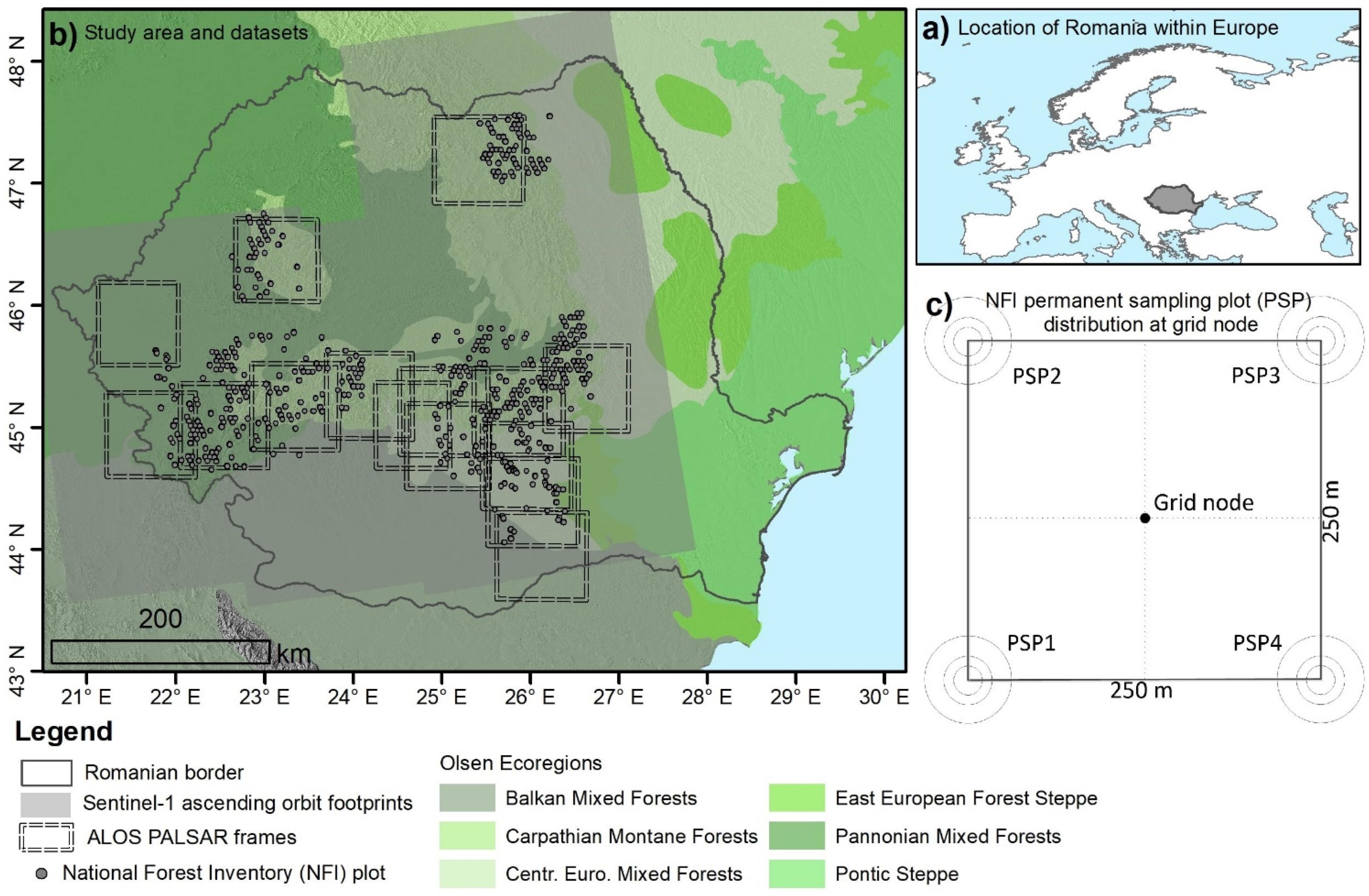
2.1. Study Area and In Situ Data

The study was carried out in selected areas of the Romanian Carpathian Mountains (Figure 1). The Carpathians is third longest range within Europe, after the Urals and the Scandinavian Mountains, and stretches 1500 km across seven countries, although most of the range (54%) is located within the Romanian borders. The Carpathians are an eastward continuation of the Alps, but differ considerably from them as they are less compact and reach lower elevations. In contrast to the Alps, glaciation affected only the highest peaks, with the remaining areas being shaped by rivers. The climate is influenced by polar-continental air from east and northeast in winter and oceanic mases from the west during the rest of the year differentiating them from the much dryer surrounding plains. Precipitations range from 600 to 1800 mm. The vegetation is dominated by forests, mainly beech, spruce, and, to a lesser extent, oak species, which provide habitats for the largest European populations of brown bears, wolves, and lynxes. The Carpathians contains most of the European Union’s remnant virgin forests. The selected areas include some of the highest mountain peaks (exceeding 2500 m) as well as three of the six ecoregions present within the Romanian national territory [31].

The in situ samples were collected within the second cycle (2013–2018) of the Romanian NFI. The NFI was established in 2008 using a 4 × 4 km grid, although a denser 2 × 2 km grid is used in plains where forest cover is low. The NFI is a two stage (aerial photography followed by in situ surveys) continuous forest inventory with a five-year cycle that covers the entire national territory. The field surveys comprise, at the end of the five-year cycle, about 24,000 permanent sample plots. To increase field work efficiency, the measurements are realized on four permanent sampling plots (PSP) at each grid node (Figure 1b). Each PSP contains three concentric circles (7.98 m, 12.62 m, and 25 m in radius) where different forest characteristics are assessed, including forest type, tree species, diameter at breast height (DBH), height (H), lying deadwood, and ground vegetation. DBH and height are assessed in the first two circles, 7.98 m (5.6 cm ≤ DBH ≤ 28.5 cm) and 12.62 m (DBH ≥ 28.5 cm). The GSV estimation is based on species-specific (43 main species) allometry based on DBH and height. For conifers, the volume of branches (>5 cm diameter) was established through specific equations as percentage of stem volume and was added to the stem volume [32]. The volume measurements are scaled (by the circle area), aggregated, and reported per hectare. NFI estimates GSV with a sampling error of 1.79%, with target differences between measurements and control surveys less than 1%. The NFI objective is to derive statistics of forest properties over the national territory. As such, individual plot measurements are not optimized to calibrate or evaluate remote sensing products due to the relatively small sampling area.

For each PSP, the data provided included the main forest species, forest inventory date, percentage forest cover, mean diameter at breast height, and height, as well as per hectare GSV. Of the 1815 PSPs available for this study, 1153 were inventoried between 2015 and 2016, coinciding with the EO data acquisition period. The remaining plots were inventoried in 2014. As forest stands in Romania consist of homogeneous tracts (species composition, age, and DBH classes), the NFI plots are representative of larger areas were not falling on stand border, as stands range between 6–10 ha in hilly and 10–15 ha in mountainous regions. The DBH, H, and GSV over the in-situ data, reached 96 cm, 50 m, and 1577 m³ ha⁻¹, respectively, depending on the sample plot (

Table 1. Range of plot-wise mean DBH and H and GSV. Values for all/modelling plots (see Section 3.1).

Main Species	DBH Range (cm)	H Range (m)	GSV Range (m3 ha−1)
beech (n = 900/322)	7–157/8–96	3–50/8–50	5–1577/9–1577
oaks (n = 249/72)	11–80/11–52	9–36/11–32	13–742/22–731
coniferous (n = 560/238)	8–85/11–85	8–44/9–43	12–1470/22–1401
other species (n = 106/33)	10–66/10–59	9–39/12–39	15–1080/15–1080

). As small pockets of large trees influence average values, when relatively small areas are assessed, the PSP-wise GSV was high (>1000 m³ ha⁻¹) for some plots (Figure 2).

2.2. Earth Observation Data

The NFI plots used in this study were covered within 13 ALOS PALSAR-2 frames and six ascending and descending Sentinel-1 relative orbits (Figure 1). 104 L-band ALOS PALSAR-2 dual-polarized (HH and HV polarizations) datasets were provided by JAXA (2014–2017 period) as single look complex (SLC) images, while 1034 Sentinel-1 A and B granules were downloaded from open repositories for the years 2015–2016, the period when most (83) ALOS PALSAR-2 datasets were acquired. Sentinel-1 ground range detected (GRD) dual polarized (VV and VH polarizations) C-band datasets (A and B satellites) were downloaded for the six relative orbits (29, 102, and 131 ascending and 7, 80, and 109 descending passes) covering the selected study areas.

3. Methods

3.1. SAR Data Processing and Extraction

The images acquired on the same orbit were first co-registered in the radar geometry. For Sentinel-1 products, the orbital state vectors were updated using the Precise Orbit Ephemerides, with the co-registration process being carried out by relative orbit after slice assembly (i.e., concatenation) as the Sentinel-1 image frames (i.e., slices) acquired from the same orbital path are provided in slices of variable ground footprints. For the ALOS PALSAR-2 data, the SAR processing was carried out on a path/frame basis. Image co-registration was based on a cross-correlation algorithm [33] with the first image of the temporal data series being used as reference. Each co-registered image was multi-looked to obtain a ground pixel spacing of approximately 30 m (4 × 8 pixels in range and azimuth for ALOS PALSAR-2 and 20 × 3 pixels in range and azimuth for Sentinel-1). The backscatter was converted to gamma0 using an ellipsoid-based area as reference, to account for the influence of topography [34]. The backscatter coefficient (γ◦) was subsequently topographically normalized using the real scattering area, derived pixel-wise [35], from the one arc-second Shuttle Radar Topography Mission (SRTM) digital elevation model (DEM). Each image was then orthorectified to the Universal Transverse Mercator (UTM) coordinate system (zone 35 North, datum WGS84) using a look-up table that related the coordinates of each pixel in the radar geometry with the coordinates of the same pixel in the map geometry. The look-up table was generated using image orbital information and the digital elevation model [36].

At each PSP, the backscatter coefficient of all images acquired before the forest inventory date was extracted for the pixel containing the center coordinates. The backscatter values were averaged for all available dates by polarization and by relative orbit (Sentinel-1). The standard deviation of the backscatter temporal series (i.e., temporal stability) was also computed at each PSP location for every sensor, polarization, and relative orbit (Sentinel-1). Out of the 1815 available NFI samples, 704 (665 forest and 39 non-forest) were used for modelling and validation of the retrieved GSV. The reduced number of useful samples was determined by the intersection between ALOS PALSAR-2 and Sentinel-1 orbits, the correspondence between NFI inventory date and ALOS PALSAR-2 and Sentinel-1 image acquisition dates, and topography, as pixels affected by geometric distortions were masked out during SAR data processing. As both ascending and descending Sentinel-1 orbits were tested, the number of PSPs affected by layover and shadow was high.

3.2. Growing Stock Volume Retrieval

Several modeling approaches can be used to retrieve forest GSV (or AGB) from radar backscatter coefficients, including parametric and nonparametric models [3,8,9,10,13,16,24,37,38,39,40,41]. Within a previous study, some of these models were evaluated using the Romanian NFI and ALOS PALSAR-2 datasets [42]. The results suggested that non-parametric models provide the lowest errors and bias, regardless of polarization or forest species over the selected study area. Therefore, we used a non-parametric modelling approach, based on Random Forests [43], to assess the synergies between the C- and L-band dataset for GSV retrieval. As non-parametric models offer the opportunity to include non-linearly related variables, and have no assumptions regarding the statistical properties of the data, such models are often preferred when a sufficiently large dataset of samples is available for model parameterization. The models use ensemble learning methods to improve the overall predictive power with respect to any of the constituent models by aggregating their predictions. In random forest regression, each tree is built using a deterministic algorithm by selecting a random set of variables and a random sample from the training dataset [43]. Although RF models provide high fit statistics there are known drawbacks, including difficulties in interpreting the results, potential overfitting, and high computational demands. A total of 85 RF models were trained and evaluated by gradually increasing the independent variables, starting from single polarized to multi-polarization multi-sensor data (see Section 4 and

Table A1. GSV accuracy as a function of the selected independent variables for a range of configurations. Abbreviations as follows: RMSE—root mean squared error, RelRMSE—relative RMSE, r—Pearson’s correlation coefficient, L—stands for L-band, C—stands for C-band, H—horizontal, V—vertical, a—ascending pass, d—descending pass, sd—standard deviation, Ft—forest type, and LIA—local incidence angle.

Independent Variables	RMSE	RelRMSE	Bias	r	Independent Variables	RMSE	RelRMSE	Bias	r
Single polarized models based on L-band data					Single polarized models based on C-band data
L-HH	282.9	66.3	3.1	0.14	Ca-VV	275.0	63.9	−2.7	0.21
					Cd-VV	277.5	64.6	−2.9	0.19
L-HH, L-HHsd	264.0	61.6	−1.1	0.24	Cd-VH, Cd-VHsd	265.0	62.7	−2.6	0.26
					Ca-VV, Ca-VVsd	262.6	62.4	−0.5	0.27
					Cd-VV, Cd-VVsd	264.6	62.8	0.36	0.26
L-HV, L-HVsd, Ft	244.0	57.1	0.02	0.41	Ca-VH, Ca-VHsd, Ft	249.0	59.2	2.1	0.38
L-HH, L-HHsd, Ft	244.2	57.6	4.3	0.40	Cd-VH, Cd-VHsd, Ft	253.7	59.8	−3.8	0.36
					Ca-VV, Ca-VVsd, Ft	248.7	59.3	1.0	0.39
					Cd-VV, Cd-VVsd, Ft	249.9	59.5	3.1	0.37
L-HV, L-HVsd, LIA	246.4	57.6	1.5	0.40	Ca-VH, Ca-VHsd, LIA	256.8	60.9	−2.0	0.31
L-HH, L-HHsd, LIA	250.7	58.8	0.75	0.37	Cd-VH, Cd-VHsd, LIA	260.0	61.2	−3.5	0.32
					Ca-VV, Ca-VVsd, LIA	257.4	61.3	1.7	0.30
					Cd-VV, Cd-VVsd, LIA	261.1	61.7	−3.5	0.30
L-HV, L-HVsd, LIA, Ft	240.3	56.2	−0.6	0.44	Ca-VH, Ca-VHsd, LIA, Ft	248.4	59.3	2.4	0.38
L-HH, L-HHsd, LIA, Ft	237.7	55.9	3.4	0.45	Cd-VH, Cd-VHsd, LIA, Ft	252.5	59.7	−0.3	0.37
					Ca-VV, Ca-VVsd, LIA, Ft	249.5	59.5	3.7	0.38
					Cd-VV, Cd-VVsd, LIA, Ft	249.8	58.6	−5.4	0.39
Multi-polarized models based on L-band data					Multi-polarized models based on C-band data
L-HV, L-HH	253.0	58.9	0.2	0.36	Ca-VV, Ca-VH	267.0	62.4	0.7	0.25
					Cd-VV, C-VH	262.0	61.1	0.2	0.27
L-HV, L-HH, L-HH/HV	251.9	59.1	2.5	0.39	Ca-VV, Ca-VH, Ca-VV/VH	264.8	61.8	3.3	0.24
					Cd-VV, Cd-VH, Cd-VV/VH	260.6	61.2	2.6	0.28
L-HV, L-HH, L-HH/HV, Ft	249.2	58.0	0.42	0.40	Ca-VV, Ca-VH, Ca-VV/VH, Ft	253.1	59.0	−1.0	0.35
					Cd-VV, Cd-VH, Cd-VV/VH Ft	248.8	58.0	−1.9	0.38
L-HV, L-HH, L-HH/HV, LIA	242.7	56.3	−2.1	0.43	Ca-VV, Ca-VH, Ca-VV/VH, LIA	253.4	59.7	6.1	0.30
					Cd-VV, Cd-VH, Cd-VV/VH, LIA	251.9	58.	−0.5	0.34
L-HV, L-HH, L-HH/HV, LIA, Ft	241.9	56.1	−3.4	0.46	Ca-VV, Ca-VH, Ca-VV/VH, LIA, Ft	252.4	58.5	−3.0	0.36
					Cd-VV, Cd-VH, Cd-VV/VH, LIA, Ft	245.7	57.0	−4.6	0.41
L-HV, L-HH/HV	252.8	58.8	−0.1	0.38	Ca-VH, Ca-VV/VH	264.2	61.5	−1.8	0.26
					Cd-VH, Cd-VV/VH	263.9	61.4	−3.5	0.27
L-HH, L-HH/HV	251.5	58.6	1.2	0.36	Ca-VV, Ca-VV/VH	265.3	62.0	0.4	0.25
					Cd-VV, Cd-VV/VH	262.3	61.3	−0.1	0.26
L-HV, L-HH/HV, LIA	242.9	56.9	2.6	0.42	Ca-VH, Ca-VV/VH, LIA	258.8	60.4	0.4	0.29
					Cd-VH, Cd-VV/VH, LIA	253.8	59.2	−1.1	0.35
L-HV, L-HH/HV, LIA, Ft	241.2	56.3	1.4	0.45	Ca-VV, Ca-VV/VH, LIA, Ft	249.2	58.1	1.4	0.36
L-HH, L-HH/HV, LIA, Ft	239.1	55.9	2.7	0.46	Cd-VV, Cd-VV/VH, LIA, Ft	246.0	57.4	−0.5	0.41
L-HV, L-HH/HV, L-HVsd	247.0	58.0	1.7	0.39	Ca-VH, Ca-VV/VH, Ca-VHsd	259.4	61.3	−2.4	0.31
L-HH, L-HH/HV, L-HHsd	248.6	58.1	−0.9	0.38	Cd-VH, Cd-VV/VH, Cd-VHsd	261.6	62.2	2.8	0.28
L-HV, L-HH/HV, L-HVsd, LIA	242.8	56.6	0.9	0.44	Ca-VH, Ca-VV/VH, Ca-VHsd, LIA	258.2	61.4	0.8	0.31
L-HV, L-HH/HV, L-HVsd, LIA, Ft	236.0	55.4	2.1	0.47	Ca-VH, Ca-VV/VH, Ca-VHsd, LIA, Ft	248.9	59.5	2.0	0.38
L-HH, L-HH/HV, L-HHsd, LIA, Ft	237.7	55.7	1.7	0.48	Cd-VH, Cd-VV/VH, Cd-VHsd, LIA, Ft	246.8	58.3	−1.3	0.42
Independent variables	RMSE	RelRMSE	Bias	r	Independent variables	RMSE	RelRMSE	Bias	r
Multi-frequency models (C- and L-band data)					Models based on C-band data from ascending and descending passes
L-HV, Ca-VV/VH	258.7	60.4	−0.3	0.32	Ca-VV, Ca-VVsd, Cd-VV, Cd-VVsd	256.9	61.2	−1.3	0.32
L-HV, Ca-VV/VH, Ft	249.0	58.1	−1.6	0.39	Ca-VH, Ca-VHsd, Cd-VH, Cd-VHsd	258.3	61.2	−3.9	0.32
L-HV, Ca-VV/VH, Cd-VV/VH	252.0	59.1	2.7	0.34	C-VVa, C-VVa sd, C-VVd, C-VVd sd, Ft	249.4	59.8	1.5	0.38
L-HV, Ca-VV/VH, Cd-VV/VH, LIA	243.2	57.2	4.9	0.41	Ca-VH, Ca-VHsd, Cd-VH, Cd-VHsd, Ft	254.2	59.8	−3.5	0.37
L-HV, L-HH/HV, Ca-VV, Ca-VV/VH, LIA	239.3	55.8	2.6	0.45	C-VVa, C-VVa sd, C-VVd, C-VVd sd, Ft, LIAa, LIAd	248.6	59.0	−1.4	0.40
L-HV, L-HH/HV, Ca-VV/VH, Cd-VV/VH, LIA	240.3	56.1	0.2	0.45	Ca-VH, Ca-VVVH, Ca-VVsd, Cd-VH. Cd-VVVH, Cd-VVsd	251.6	60.0	1.9	0.34
L-HV, L-HH/HV, Ca-VV/VH, Ca-VHsd, Cd-VV/VH, Cd-VHsd, LIA	242.3	57.6	−0.3	0.46	Ca-VV, Ca-VVVH, Cd-VV, Cd-VVVH, Ca-VHsd, Cd-VHsd	254.6	60.7	0.6	0.33
L-HV, L-HH/HV, Ca-VH, Ca-VV/VH, Cd-VH, Cd-VV/VH, LIA	240.1	57.3	1.2	0.46

in Appendix A for detailed information of the predictor variables used). Each sensor was individually tested to generate a reference baseline and allow for cross-sensor comparisons. The use of additional variables (e.g., forest type, temporal backscatter variability, and local incidence angle) was also evaluated to ascertain the opportunity for GSV retrieval improvements. For each sensor, we increased the independent variables, starting with the average backscatter, temporal stability (i.e., the standard deviation of the time series, sd), local incidence angle (LIA), and the forest type (Ft). For the C-band we analyzed the ascending and descending passes separately, as well as their combination. The models were calibrated using the 704 PSP samples. In this study, TreeBagger from MATLAB^® software package (v. 2020b) was used to construct the RF classifier. The number of decision trees was set to 200 and a curvature test was used to select the best split predictor and grow unbiased trees [44]. The remaining parameters were kept as default, with surrogate splits being allowed to account for missing values in the data.

3.3. GSV Retrieval Accuracy

Model performance was evaluated at both pixel and grid levels. At pixel (i.e., plot) level, the retrieval was evaluated using repeat random sub-sampling with cross-validation for each individual sensor and polarization, as well as for dual polarized and dual frequency configurations. To reduce variability due to random sampling effects, 100 rounds were performed by randomly splitting the 704 PSPs into training (75%) and validation (25%) samples. During each round, the models were calibrated using the training samples and subsequently used to estimate the GSV for the validation samples. The observed and predicted GSV for the validation samples was accumulated over the 100 rounds and used to compute four accuracy error metrics: the root mean squared error (RMSE, Equation (1)), the relative RMSE (RelRMSE, Equation (2)), the bias (Equation (3)), and the Pearson’s correlation coefficient (r).

$$RMSE=\sqrt{\frac{1}{n}{\displaystyle \sum }_{j=1}^n{\left(P_j-O_j\right)}^2}$$

(1)

$$RelRMSE=RMSE/\tilde{O}$$

(2)

$$Bias=\tilde{P}-\tilde{O}$$

(3)

where: P_j = predicted values, O_j = in situ observed values, n = number of samples, and $\tilde{O}$ and $\tilde{P}$ = mean values for the observed and predicted values, respectively.

As GSV estimation errors are inherently large when using small NFI plots for SAR models calibration [45,46], accuracy metrics (as per Equations (1)–(3)) were also derived over predefined grids of 10 × 10, 20 × 20, and 30 × 30 km. The grid size was a compromise between having enough samples in each tile to obtain a more reliable estimate of the NFI average stem volume and having enough tiles to compute the accuracy metrics by volume intervals. As the Sentinel-1 strips covered the 1815 available PSPs (Figure 1), the analysis was focused on the GSV maps derived from C-band VH polarized data (see Section 4.2) to maximize the number of tiles containing at least 4 in situ plots (i.e., one NFI grid node). The errors were estimated for both ascending and descending satellite passes. Models using the VH backscatter and its temporal standard deviation (see Table 2, in bold) were calibrated using the reduced set (704) of NFI for cross-comparison purposes. At each tile, the average NFI GSV was compared to the average GSV for the corresponding predicted pixels.

3.4. Local vs. Global GSV Retrieval

The GSV overall accuracy estimates were compared against values derived at continental to global levels. We used the GlobBiomass dataset [20], the only global product currently available at comparable pixel spacing (100 m) and derived from comparable remote sensing datasets (C- and L-band SAR data). The GlobBiomass product provides GSV estimates for the reference year 2010 based on the combined use of Envisat ASAR (C-band) and ALOS PALSAR (L-band) sensors and ancillary information from Landsat imagery. GSV values from the first NFI cycle (2008–2012) were used as reference to match the dates of the GlobBiomass product. As NFI data collection protocol and location did not change between the first and second NFI cycles and we have used the same SAR wavelengths to derive the local product, input datasets influence on the results were minimized. Please note that Envisat ASAR and ALOS PALSAR sensors were decommissioned in 2012 and 2011, respectively while data from Sentinel-1 and ALOS PALSAR-2 were not available until 2014. The GlobBiomass GSV values were extracted at the location of the available NFI plots to compute the same error metrics.

4. Results and Discussions

The higher backscatter variability at L-band when compared to C-band, due to the limited number of multi-temporal datasets available is evident for all the main species in the Carpathians (Figure 3). Additionally, notice the different GSV ranges, significantly larger for beech forests when compared to the coniferous and oak forests. The backscatter coefficient shows the specific raise with GSV up to a SAR wavelength specific saturation point. By main species, the average backscatter values were slightly higher at L-band over the coniferous forests (Figure 3b). For display reasons, a logarithmic model was fitted to the data. The fit was very similar for both SAR wavelengths over the high biomass beech forests (Figure 3c). Different saturation points between the two wavelengths are apparent over the coniferous and oak forests (Figure 3b,d), suggesting changed sensitivity to GSV.

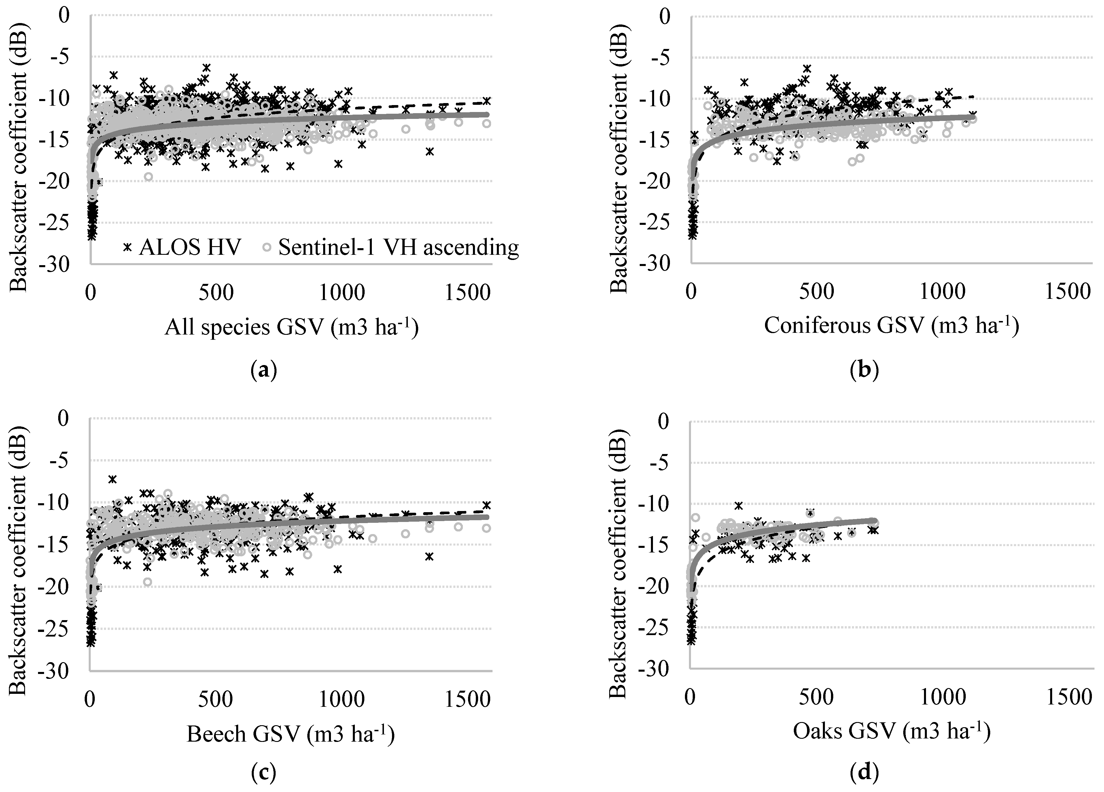
4.1. Pixel-Wise GSV Estimation

Over all sensors, polarizations, and predictor variables combinations, the RMSE, Rel RMSE, and r ranged between 238–278 m³ ha⁻¹, 55–65%, −5–6 m³ ha⁻¹, and 0.14–0.48, respectively (

Table 2. GSV accuracy as a function of the independent variables used for the single polarized models. Bold numbers show overall results for the models analyzed by GSV intervals in Figure 4 and Figure 5. Abbreviations as follows: RMSE—root mean squared error, RelRMSE—relative RMSE, r—Pearson’s correlation coefficient, L—stands for L-band, C—stands for C-band, H—horizontal, V—vertical, a—ascending pass, d—descending pass, sd—standard deviation, Ft—forest type, and LIA—local incidence angle.

Independent Variables	RMSE	RelRMSE	Bias	r	Independent Variables	RMSE	RelRMSE	Bias	r
L-HV	266.9	62.4	−1.4	0.30	Ca-VH	274.0	63.9	−0.3	0.24
L-HH	282.9	66.3	3.1	0.14	Ca-VV	275.0	63.9	−2.7	0.21
L-HV, L-HVsd	254.3	59.5	−1.4	0.35	Ca-VH, Ca-VHsd	263.4	62.6	−0.3	0.28
L-HV, L-HH	253.0	58.9	0.2	0.36	Ca-VV, Ca-VH	267.0	62.4	0.7	0.25
L-HV, L-HVsd, Ft	244.0	57.1	0.02	0.41	Ca-VH, Ca-VHsd, Ft	249.0	59.2	2.1	0.38
L-HV, L-HH, L-HH/HV, LIA, Ft	241.9	56.1	−3.4	0.46	Cd-VV, Cd-VH, Cd-VV/VH, LIA, Ft	245.7	57.0	−4.6	0.41
L-HV, L-HH/HV, Ca-VH, Ca-VV/VH, LIA	239.9	56.2	1.9	0.45	Ca-VH, Ca-VHsd, Cd-VH, Cd-VHsd, Ft, LIAa, LIAd	249.5	59.5	−0.6	0.40

and Table A1). As showing results for all possible combinations of the predictor variables (19) is problematic, Table 2 shows the error metrics for a selection of models to understand their variations when expanding the number of predictor variables. Notice that adding more variables does not translate into more accurate predictions. Additional configurations were provided in Table A1 for completeness. The data is presented by SAR wavelength, multi-frequency configurations and descending C-band passes combinations.

Within the single sensor single polarization configuration, the L-band data provided similar relative RMSE errors when compared to the C-band data. The small difference was explained by the much denser C-band time series, and the use of average backscatter over 3 years prior to the forest inventory date. This allowed for a considerable reduction in the environmental induced noise (i.e., backscatter variation due to changes in soil and vegetation water content) at C-band, where over 150 images were averaged over each relative orbit. In contrast, fewer images (5–10) were available for the ALOS PALSAR-2 sensor over each acquisition frame. Improved GSV retrieval accuracy at C-band was observed when adding as an independent variable either the local incidence angle (LIA) or the forest type (FT). However, such improvements were marginal for all accuracy metrics. The RMSE, RelRMSE, and r improved, on average, by 15 m³ ha⁻¹, 3%, and 0.1, respectively. Dual polarized models were slightly more accurate (2–5%) when compared to single polarized models at both C- and L-bands, while the addition of co- to cross-polarized backscatter ratios further decreased the estimation error, albeit marginally. Adding the time series standard deviation to backscatter and co- to cross-polarized ratios improved the accuracy metrics slightly, suggesting that some information can be added to that already contained in the backscatter coefficient. Similarly, adding LIA and/or FT to the models only resulted in marginal improvement, most likely being related to the increased number of variables available in the model. No synergies were observed in terms of retrieval accuracy, when combining information from both ascending and descending C-band passes with model performance not improving over the use of either pass. However, GSV estimation from both ascending and descending passes has merit over the rough Carpathian topography, as it limits the extent of ‘not-observed’ areas, i.e., areas with topographic distortion due to shadows and layover which are masked out during SAR processing. Further, the similar error level from both passes provides for a homogeneous GSV estimation over the entire landscape. Little synergy was also observed when simultaneously using C- and L-band for GSV retrieval. Improvements in the RMSE, RelRMSE, and r were noticed with respect to using single pass C-band data, but were marginal, i.e., 10 m³/ha, 3%, and 0.05, respectively. In addition, such improvements were observed when adding the LIA to the various combinations of SAR frequencies, polarizations, and passes. The information provided by LIA and Ftype was largely interchangeable in all configurations (single, dual, multi-frequency, and multi-pass), as simultaneously using both variables did not improve the results. In fact, the opposite was observed for some of the tested combinations. It seems that LIA partitions data in a similar way to Ftype as oak forests are mostly found on lesser slopes in the hilly region, with conifers being found towards the mountain tops on steep terrain. This explanation is further supported by the fact that adding the LIA from different sensors or satellite passes provided no tangible improvement of the accuracy metrics.

Error analysis by intervals (Figure 4 for models in bold in Table 2) shows much higher relative RMSE errors over forests supporting low (<100 m³ ha⁻¹) GSV values at both C- and L-bands, which is consistent with previous findings [14,47]. The high relative RMSE are related to the high signal variability due to the influence of local surface conditions (i.e., soil surface roughness and moisture) as direct scattering from the ground dominates the signal in forests supporting low GSV levels [48]. In addition, the relative RMSE metric is unstable at lower GSV values, as the denominator approaches zero the relative error approaches infinity. Over the remaining GSV intervals the relative RMSE decreased significantly at both wavelengths with the minimum values (around 20%) being observed for the 400–600 m³ ha⁻¹ GSV range. The estimation error was largely dominated by bias, as the coefficient of variation (CV) of the error was below one (data not shown), for most GSV intervals except the 400–600 m³ ha⁻¹ where the random error dominated, and the 0–100 m³ ha⁻¹ interval where bias and random error contribution was balanced (0.8 < CV < 0.9). Note that the bias was positive over low GSV ranges and negative over the high GSV ranges (Figure 5b), with a crossover at the GSV range with the lowest errors, 400–600 m³ ha⁻¹. The standard deviation (SD) of the predicted values did not vary across GSV intervals (75–85 m³ ha⁻¹) except for the first bin, where the SD was twice as much (Figure 5a). Similar values were observed over temperate forests in Poland in previous studies [14]. Overall, the accuracy assessment shows that GSV is over- and under-estimated at low and high GSV values, respectively as the models fitting aims at the point defined by the average of the observed and predicted values [14].

The relatively large errors observed for all combinations of predictor variables may be related to potential mismatches between the Earth Observation data and the in situ samples, as the coordinates at each PSP were reconstructed from the node grid coordinates using the specified distance and azimuth. This may introduce displacements with respect to the real location of the NFI plot where field crews were not able to precisely measure the required azimuth and distance, or the exact location of the grid node (e.g., GPS location error under dense forest canopy may reach several meters). Such positioning errors coupled with the relatively small area inventoried may induce errors particularly for border stands. For the remaining NFI samples, the positioning errors should have limited effects as Romanian forests stands, averaging between 3.5 and 15 ha from plains to mountains, have homogeneous structure and species composition.

4.2. Grid Based GSV Accuracy

Over the 10 × 10 km grid (244 cells), the RMSE and RelRMSE decreased to 158 m³ ha⁻¹ and 35%, respectively (average values), with marginal differences being observed between values from ascending (35.2%) and descending (33.8%) satellite passes. Averaging GSV values from ascending and descending passes did not result in improved accuracy metrics. Further aggregation through the larger 20 × 20 (125 cells) and 30 × 30 km (78 cells) grids improved RMSE (119 and 105 m³ ha⁻¹, respectively) and RelRMSE (29% and 25%, respectively) values, but also increased the bias from 13 to 30 and, 35 m³ ha⁻¹, respectively, as only two or three bins were available. The RelRMSE for the 30 × 30 km aggregation level was similar to that observed over the Swedish forests (21.4%) at the same scale. However, our retrieval statistics indicate some residual bias, which was not the case in Sweden, where a longer wavelength (L-band) was used for retrieval and more samples were aggregated [49].

When compared to the pixel-based assessment, similar patterns were observed over all biomass intervals except for the 0–100 m³ ha⁻¹ range for which no grid cell was available (Figure 5 for models in bold in Table 2). The improvement in retrieval statistics seemd related to the absence of low GSV plots (<100 m³ ha⁻¹) where large estimation errors were observed at pixel level (Figure 4 and Figure 5). Notice that the lower number of available cells at larger grids precluded a similar analysis for the 20 × 20 and 30 × 30 km grids.

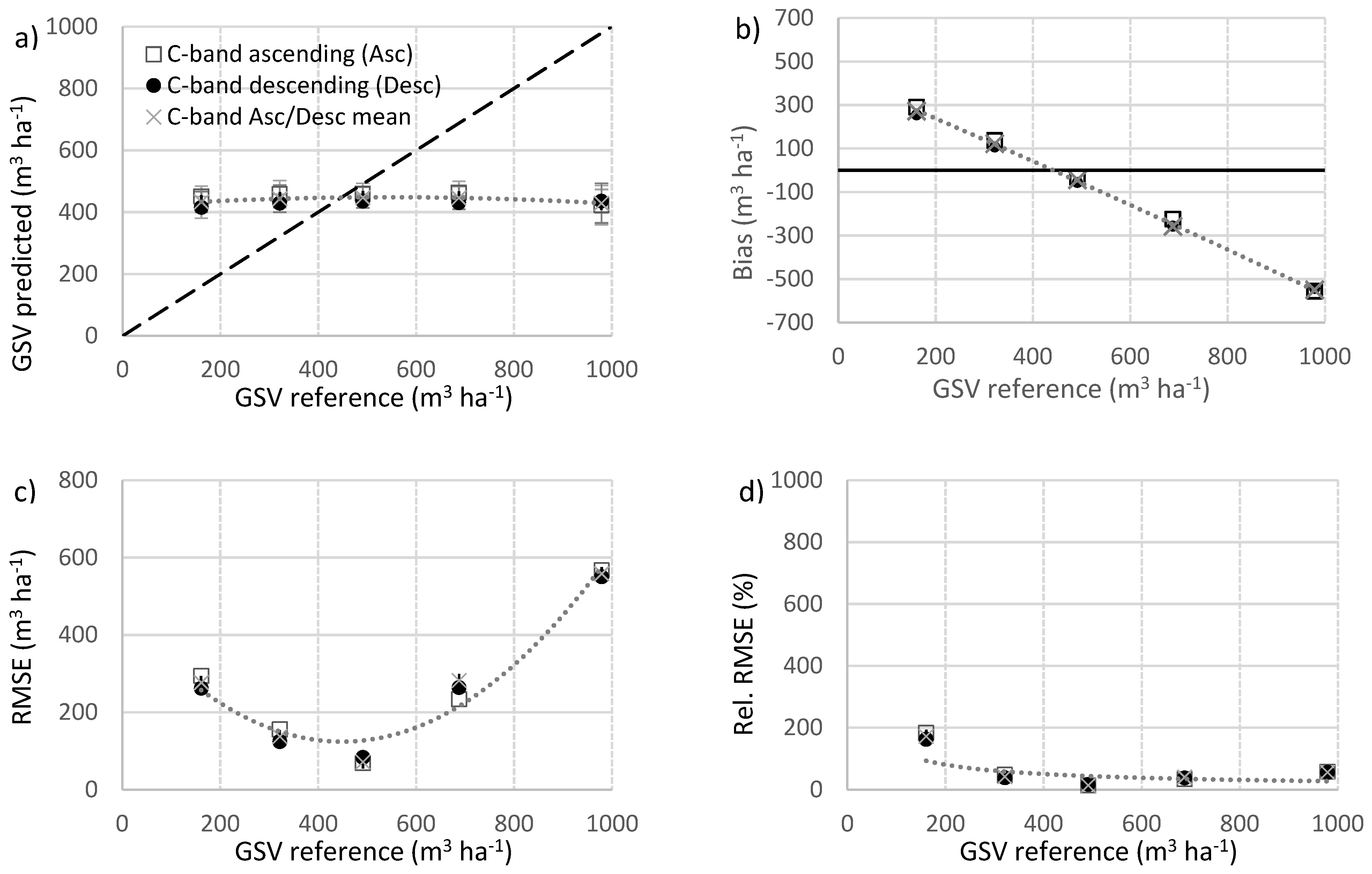
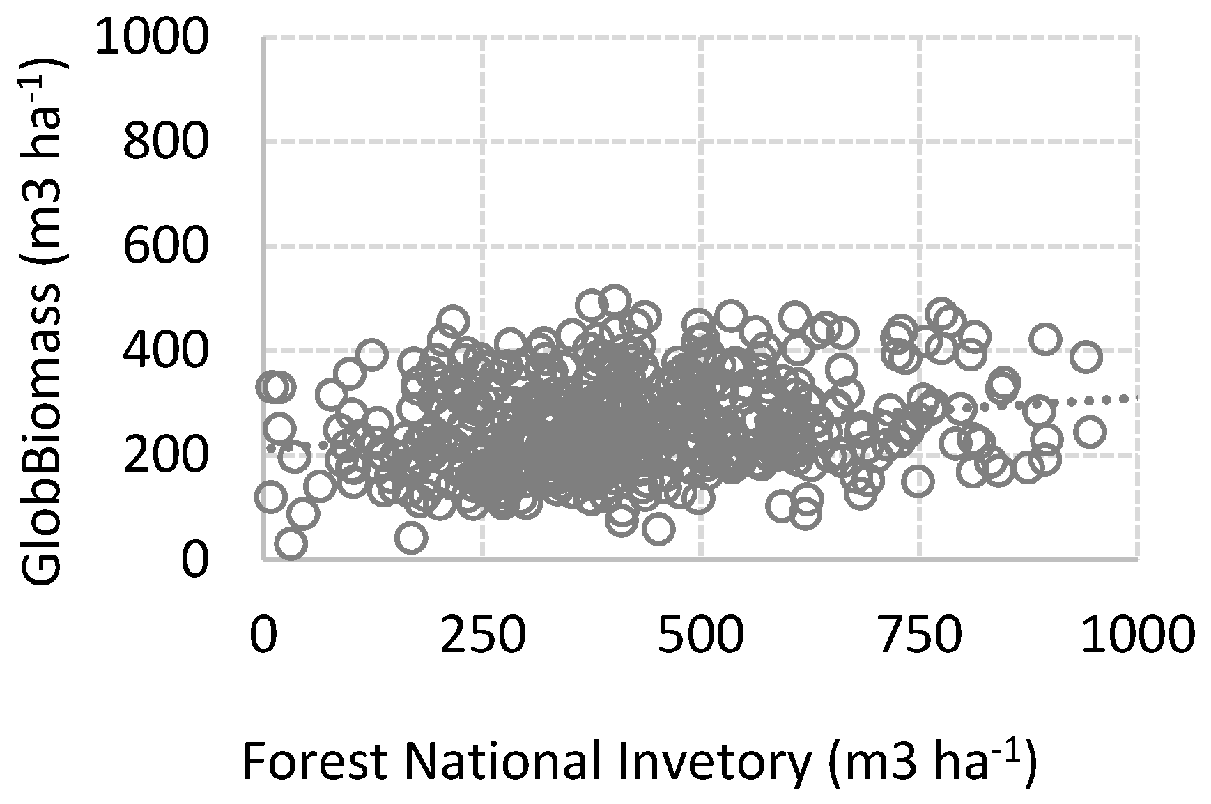
4.3. Comparison to Global Products

Our results support previous findings which demonstrated increased retrieval accuracies for locally calibrated models [14,23,24,25]. When compared to the GlobBiomass values (Figure 6), locally derived estimates showed potential to improve the RelRMSE by about 15% (55.4 vs. 70.5%), decrease the RMSE by about 54 m³ ha⁻¹ (236 vs. 290 m³/ha), and increase the correlation between predicted and observe values from 0.2 to 0.5. Such improvements, although significant and at a higher (30 vs. 100 m) spatial resolution, are still far from the required accuracies needed for operational forest management which target 5–10% accuracies for GSV at stand level. Nevertheless, one should notice that aggregating the pixel wise GSV to lower spatial resolution (e.g., stand level) has the potential to significantly decrease the RMSE and RelRMSE values [13,50] as also demonstrated by the improvements observed at grid level. The incentive in using SAR based GSV estimation from locally calibrate models resides in the opportunity to better fine tune the model to the local conditions when compared to using globally available estimate. In addition, SAR-based maps provide wall to wall cover, yearly updates, and the opportunity to derive regional statistics.

5. Conclusions

This study assessed the utility of C- and L-band data for GSV estimation over high growing stock volume forests in the Carpathians. The study included representative areas covering the three main forest species, oak, beech, and coniferous, making up the bulk of the Romanian forests. The in situ NFI data and the SAR imagery were acquired between 2015 and 2016. GSV retrieval was carried out at 30 m pixel size using a machine learning (Random Forests) algorithm and various configurations of the independent variables from single sensor single polarization to multi-sensor multi-polarization. The observed RelRMSE varied between 55–66% depending on the input predictor variables. For similar predictor variables, the mapping accuracy was slightly higher at L- when compared to C-band.

The availability of significantly more datasets at C-band reduced speckle as the much denser Sentinel-1 time series seemed to have compensated for the inherent limitations of a shorter wavelength. Such a finding suggests that using denser L-band time series, as those available from the soon to be launched NISAR mission, have the potential to further improve GSV estimation accuracy in high volume forests. The GSV retrieval errors decreased by 5–10% when adding temporal information (i.e., backscatter coefficient temporal standard deviation) as an independent variable eliminating the need for a second polarization. This suggests a high correlation between the information of co- and cross-polarized channels, which may be explained by the overall high GSV levels and thus the relative low correlation between GSV and backscatter. Little synergies were observed when using both C- and L-bands, as well as when jointly using C-band ascending and descending passes. While the utility of the pixel level GSV values is somewhat reduced, their aggregation at grid level decreased the estimation errors (25–35%) and provided more reliable estimates which may be useful for regional and national assessments. Future work should focus on reducing GSV errors by fusing the Lidar data acquired by NASA’s Global Ecosystem Dynamics Investigation (GEDI) mission to obtain a GSV gridded product that provides more accurate estimates for stock levels at regional to national levels. In addition, dense L-band temporal series from the future NISAR mission should be tested to ascertain the potential to improve the locally derived GSV estimates, as datasets from the P-band BIOMASS mission may not be available over the Carpathians.

As for the limitations of this study, the most important is related to the design of NFIs, which are not optimized for calibrating and validating remote sensing products [49], the large differences between the amount of data collected by the two SAR sensors, which limited a like-for-like comparison, and the available DEM (SRTM DEM) used for terrain normalization as a more precise DEM (e.g., Lidar based or Tandem-X DEM) allows for improved scattering area estimation reducing the effect of topography on the backscatter and thus improving the retrieval of the target biophysical characteristic [34,51].

References

1. Gibbs, H.K.; Brown, S.; Niles, J.O.; Foley, J.A. Monitoring and estimating tropical forest carbon stocks: Making redd a reality. Environ. Res. Lett. 2007, 2, 1–13. [Google Scholar] [CrossRef]
2. Breidenbach, J.; Granhus, A.; Hylen, G.; Eriksen, R.; Astrup, R. A century of national forest inventory in norway—Informing past, present, and future decisions. For. Ecosyst. 2020, 7, 46. [Google Scholar] [CrossRef] [PubMed]
3. Santoro, M.; Cartus, O. Research pathways of forest above-ground biomass estimation based on sar backscatter and interferometric sar observations. Remote Sens. 2018, 10, 608. [Google Scholar] [CrossRef] [Green Version]
4. Tanase, M.A.; de la Riva, J.; Santoro, M.; Pérez-Cabello, F.; Kasischke, E. Sensitivity of sar data to post-fire forest regrowth in mediterranean and boreal forests. Remote Sens. Environ. 2011, 115, 2075–2085. [Google Scholar] [CrossRef]
5. Nelson, R.F.; Hyde, P.; Johnson, P.; Emessiene, B.; Imhoff, M.L.; Campbell, R.; Edwards, W. Investigating radar–lidar synergy in a north carolina pine forest. Remote Sens. Environ. 2007, 110, 98–108. [Google Scholar] [CrossRef]
6. Tanase, M.; Ismail, I.; Lowell, K.; Karyanto, O.; Santoro, M. Detecting and quantifying forest change: The potential of existing c- and x-band radar datase. PLoS ONE 2015, 10, e0131079. [Google Scholar] [CrossRef]
7. Santoro, M.; Askne, J.; Smith, G.; Fransson, J.E.S. Stem volume retrieval in boreal forests from ers-1/2 interferometry. Remote Sens. Environ. 2002, 81, 19–35. [Google Scholar] [CrossRef]
8. Sandberg, G.; Ulander, L.M.H.; Fransson, J.E.S.; Holmgren, J.; Toan, T.L. L- and p-band backscatter intensity for biomass retrieval in hemiboreal forest. Remote Sens. Environ. 2011, 115, 2874–2886. [Google Scholar] [CrossRef]
9. Mitchard, E.T.A.; Saatchi, S.S.; White, L.J.T.; Abernethy, K.A.; Jeffery, K.J.; Lewis, S.L.; Collins, M.; Lefsky, M.A.; Leal, M.E.; Woodhouse, I.H.; et al. Mapping tropical forest biomass with radar and spaceborne lidar in lope national park, gabon: Overcoming problems of high biomass and persistent cloud. Biogeosceinces 2011, 9, 179–191. [Google Scholar] [CrossRef] [Green Version]
10. Neumann, M.; Saatchi, S.S.; Ulander, L.M.H.; Fransson, J.E.S. Assessing performance of l- and p-band polarimetric interferometric sar data in estimating boreal forest above-ground biomass. IEEE Trans. Geosci. Remote Sens. 2012, 50, 714–726. [Google Scholar] [CrossRef]
11. Askne, J.I.H.; Fransson, J.E.S.; Santoro, M.; Soja, M.J.; Ulander, L.M.H. Model-based biomass estimation of a hemi-boreal forest from multitemporal tandem-x acquisitions. Remote Sens. 2013, 5, 5574–5597. [Google Scholar] [CrossRef] [Green Version]
12. Tanase, M.A.; Panciera, R.; Lowell, K.; Aponte, C.; Hacker, J.M.; Walker, J.P. Forest biomass estimation at high spatial resolution: Radar vs. Lidar sensors. IEEE Trans. Geosci. Remote Sens. Lett. 2014, 11, 711–715. [Google Scholar] [CrossRef]
13. Santoro, M.; Beaudoin, A.; Beer, C.; Cartus, O.; Fransson, J.E.S.; Hall, R.J.; Pathe, C.; Schmullius, C.; Schepaschenko, D.; Shvidenko, A.; et al. Forest growing stock volume of the northern hemisphere: Spatially explicit estimates for 2010 derived from envisat asar. Remote Sens. Environ. 2015, 168, 316–334. [Google Scholar] [CrossRef]
14. Rodríguez-Veiga, P.; Quegan, S.; Carreiras, J.; Persson, H.J.; Fransson, J.E.S.; Hoscilo, A.; Ziółkowski, D.; Stereńczak, K.; Lohberger, S.; Stängel, M.; et al. Forest biomass retrieval approaches from earth observation in different biomes. Int. J. Appl. Earth Obs. Geoinf. 2019, 77, 53–68. [Google Scholar] [CrossRef]
15. Baccini, A.; Laporte, N.; Goetz, S.J.; Sun, M.; Dong, H. A first map of tropical africa’s above-ground biomass derived from satellite imagery. Environ. Res. Lett. 2008, 3, 45001. [Google Scholar] [CrossRef] [Green Version]
16. Saatchi, S.S.; Harris, N.L.; Brown, S.; Lefsky, M.; Mitchard, E.T.A.; Salas, W.; Zutta, B.R.; Buermann, W.; Lewis, S.L.; Hagen, S.; et al. Benchmark map of forest carbon stocks in tropical regions across three continents. Proc. Natl. Acad. Sci. USA 2011, 108, 9899–9904. [Google Scholar] [CrossRef] [Green Version]
17. Thurner, M.; Beer, C.; Santoro, M.; Carvalhais, N.; Wutzler, T.; Schepaschenko, D.; Shvidenko, A.; Kompter, E.; Ahrens, B.; Levick, S.R.; et al. Carbon stock and density of northern boreal and temperate forests. Glob. Ecol. Biogeogr. 2014, 23, 297–310. [Google Scholar] [CrossRef]
18. Avitabile, V.; Herold, M.; Heuvelink, G.B.M.; Lewis, S.L.; Phillips, O.L.; Asner, G.P.; Armston, J.; Ashton, P.S.; Banin, L.; Bayol, N.; et al. An integrated pan-tropical biomass map using multiple reference datasets. Glob. Chang. Biol. 2016, 22, 1406–1420. [Google Scholar] [CrossRef] [Green Version]
19. Hu, T.; Su, Y.; Xue, B.; Liu, J.; Zhao, X.; Fang, J.; Guo, Q. Mapping global forest aboveground biomass with spaceborne lidar, optical imagery, and forest inventory data. Remote Sens. 2016, 8, 565. [Google Scholar] [CrossRef] [Green Version]
20. Santoro, M.; Cartus, O.; Carvalhais, N.; Rozendaal, D.; Avitabilie, V.; Araza, A.; de Bruin, S.; Herold, M.; Quegan, S.; Rodríguez Veiga, P.; et al. The global forest above-ground biomass pool for 2010 estimated from high-resolution satellite observations. Earth Syst. Sci. Data Discuss. 2020, 2020, 1–38. [Google Scholar]
21. Mitchard, E.T.A.; Saatchi, S.S.; Lewis, S.L.; Feldpausch, T.R.; Woodhouse, I.H.; Sonké, B.; Rowland, C.; Meir, P. Measuring biomass changes due to woody encroachment and deforestation/degradation in a forest–savanna boundary region of central africa using multi-temporal l-band radar backscatter. Remote Sens. Environ. 2011, 115, 2861–2873. [Google Scholar] [CrossRef] [Green Version]
22. Tropek, R.; Sedláček, O.; Beck, J.; Keil, P.; Musilová, Z.; Šímová, I.; Storch, D. Comment on “high-resolution global maps of 21st-century forest cover change”. Science 2014, 344, 981. [Google Scholar] [CrossRef] [Green Version]
23. Rodríguez-Veiga, P.; Saatchi, S.; Tansey, K.; Balzter, H. Magnitude, spatial distribution and uncertainty of forest biomass stocks in mexico. Remote Sens. Environ. 2016, 183, 265–281. [Google Scholar] [CrossRef] [Green Version]
24. Michelakis, D.; Stuart, N.; Lopez, G.; Linares, V.; Woodhouse, I.H. Local-scale mapping of biomass in tropical lowland pine savannas using alos palsar. Forest 2014, 5, 2377–2399. [Google Scholar] [CrossRef] [Green Version]
25. Næsset, E.; McRoberts, R.E.; Pekkarinen, A.; Saatchi, S.; Santoro, M.; Trier, Ø.D.; Zahabu, E.; Gobakken, T. Use of local and global maps of forest canopy height and aboveground biomass to enhance local estimates of biomass in miombo woodlands in tanzania. Int. J. Appl. Earth Obs. Geoinf. 2020, 93, 102138. [Google Scholar] [CrossRef]
26. Knorn, J.; Kuemmerle, T.; Radeloff, V.C.; Szabo, A.; Mindrescu, M.; Keeton, W.S.; Abrudan, I.; Griffiths, P.; Gancz, V.; Hostert, P. Forest restitution and protected area effectiveness in post-socialist romania. Biol. Conserv. 2012, 146, 204–212. [Google Scholar] [CrossRef]
27. Schimel, D.; Melillo, J.; Tian, H.; McGuire, A.D.; Kicklighter, D.; Kittel, T.; Rosenbloom, N.; Running, S.; Thornton, P.; Ojima, D.; et al. Contribution of increasing co2 and climate to carbon storage by ecosystems in the united states. Science 2000, 287, 2004–2006. [Google Scholar] [CrossRef]
28. Scheller, R.M.; Mladenoff, D.J. A spatially interactive simulation of climate change, harvesting, wind, and tree species migration and projected changes to forest composition and biomass in northern wisconsin, USA. Glob. Chang. Biol. 2005, 11, 307–321. [Google Scholar] [CrossRef]
29. Griffiths, P.; Kuemmerle, T.; Kennedy, R.E.; Abrudan, I.V.; Knorn, J.; Hostert, P. Using annual time-series of landsat images to assess the effects of forest restitution in post-socialist romania. Remote Sens. Environ. 2012, 118, 199–214. [Google Scholar] [CrossRef]
30. Potapov, P.V.; Turubanova, S.A.; Tyukavina, A.; Krylov, A.M.; McCart, J.L.; Radeloff, V.C.; Hansen, M.C. Eastern europe’s forest cover dynamics from 1985 to 2012 quantified from the full landsat archive. Remote Sens. Environ. 2015, 159, 28–43. [Google Scholar] [CrossRef]
31. Olson, D.M.; Dinerstein, E.; Wikramanayake, E.D.; Burgess, N.D.; Powell, G.V.N.; Underwood, E.C.; D’amico, J.A.; Itoua, I.; Strand, H.E.; Morrison, J.C.; et al. Terrestrial ecoregions of the world: A new map of life on earth: A new global map of terrestrial ecoregions provides an innovative tool for conserving biodiversity. BioScience 2001, 51, 933–938. [Google Scholar] [CrossRef]
32. Giurgiu, V.; Decei, I.; Drăghiciu, D. Forest Mensuration Methods and Tables; Ed. Ceres: Bucuresti, Romania, 2004. [Google Scholar]
33. Werner, C.; Wegmuller, U.; Strozzi, T.; Wiesmann, A. Precision estimation of local offsets between pairs of sar slcs and detected sar images. In Proceedings of the Geoscience and Remote Sensing Symposium, Seoul, Korea, 25–29 July 2005; pp. 4803–4805. [Google Scholar]
34. Small, D. Flattening gamma: Radiometric terrain correction for sar imagery. IEEE Trans. Geosci. Remote Sens. 2011, 49, 3081–3093. [Google Scholar] [CrossRef]
35. Frey, O.; Santoro, M.; Werner, C.L.; Wegmüller, U. Dem-based sar pixel-area estimation for enhanced geocoding refinement and radiometric normalization. Geosci. Remote Sens. Lett. IEEE 2013, 10, 48–52. [Google Scholar] [CrossRef]
36. Wegmüller, U.; Werner, C.; Strozzi, T.; Wiesmann, A. Automated and precise image registration procedures. In Analysis of Multi-Temporal Remote Sensing Images; Bruzzone, L., Smits, P., Eds.; World Scientific: Singapore, 2002; Volume 2, pp. 37–49. [Google Scholar]
37. Lucas, R.; Armston, J.; Fairfax, R.; Fensham, R.; Accad, A.; Carreiras, J.; Kelley, J.; Bunting, P.; Clewley, D.; Bray, S.; et al. An evaluation of the alos palsar l-band backscatter—Above ground biomass relationship queensland, australia: Impacts of surface moisture condition and vegetation structure. IEEE J. Sel. Top. Appl. Earth Obs. Remote Sens. 2010, 3, 576–593. [Google Scholar] [CrossRef]
38. Englhart, S.; Keuck, V.; Siegert, F. Aboveground biomass retrieval in tropical forests—The potential of combined x- and l-band sar data use. Remote Sens. Environ. 2011, 115, 1260–1271. [Google Scholar] [CrossRef]
39. Cartus, O.; Santoro, M.; Kellndorfer, J. Mapping forest aboveground biomass in the northeastern united states with alos palsar dual-polarization l-band. Remote Sens. Environ. 2012, 124, 466–478. [Google Scholar] [CrossRef]
40. Mermoz, S.; Réjou-Méchain, M.; Villard, L.; Toan, T.L.; Rossi, V.; Gourlet-Fleury, S. Decrease of l-band sar backscatter with biomass of dense forests. Remote Sens. Environ. 2015, 159, 307–317. [Google Scholar] [CrossRef]
41. Villard, L.; Le Toan, T.; Ho Tong Minh, D.; Mermoz, S.; Bouvet, A. Forest biomass from radar remote sensing. In Land Surface Remote Sensing in Agriculture and Forest; Zribi, M., Ed.; Elsevier: Amsterdam, The Netherlands, 2016; pp. 363–425. [Google Scholar]
42. Tanase, M.A.; Marin, G.; Belenguer-Plomer, M.A.; Borlaf, I.; Popescu, F.; Badea, O. Deep neural networks for forest growing stock volume retrieval: A comparative analysis for l-band sar data. In Proceedings of the IGARSS 2020–2020 IEEE International Geoscience and Remote Sensing Symposium, Waikoloa, HI, USA, 26 September–2 October 2020; pp. 4975–4978. [Google Scholar]
43. Breiman, L. Random forests. Mach. Learn. 2001, 45, 5–32. [Google Scholar] [CrossRef] [Green Version]
44. Loh, W.Y. Regression trees with unbiased variable selection and interaction detection. Stat. Sin. 2002, 12, 361–386. [Google Scholar]
45. Robinson, C.; Saatchi, S.; Neumann, M.; Gillespie, T. Impacts of spatial variability on aboveground biomass estimation from l-band radar in a temperate forest. Remote Sens. 2013, 5, 1001–1023. [Google Scholar] [CrossRef] [Green Version]
46. Tanase, M.; Panciera, R.; Lowell, K.; Tian, S.; Hacker, J.; Walker, J.P. Airborne multi temporal l-band polarimetric sar data for forest biomass estimation in semi-arid forests. Remote Sens. Environ. 2014, 145, 93–104. [Google Scholar] [CrossRef]
47. Tanase, M.A.; Panciera, R.; Lowell, K.; Tian, S.; Garcia-Martin, A.; Walker, J.P. Sensitivity of l-band radar backscatter to forest biomass in semi-arid environments: A comparative analysis of parametric and non-parametric models. IEEE Trans. Geosci. Remote Sens. 2014, 52, 1–15. [Google Scholar] [CrossRef]
48. van Zyl, J.J. Unsupervised classification of scattering behavior using radar polarimetry data. IEEE Trans. Geosci. Remote Sens. 1989, 27, 36–45. [Google Scholar] [CrossRef]
49. Santoro, M.; Cartus, O.; Fransson, J.E.S. Integration of allometric equations in the water cloud model towards an improved retrieval of forest stem volume with l-band sar data in sweden. Remote Sens. Environ. 2021, 253, 112235. [Google Scholar] [CrossRef]
50. Santoro, M.; Beer, C.; Cartus, O.; Schmullius, C.; Shvidenko, A.; McCallum, I.; Wegmüller, U.; Wiesmann, A. Retrieval of growing stock volume in boreal forest using hyper-temporal series of envisat asar scansar backscatter measurements. Remote Sens. Environ. 2011, 115, 490–507. [Google Scholar] [CrossRef]
51. Borlaf-Mena, I.; Santoro, M.; Villard, L.; Badea, O.; Tanase, M.A. Investigating the impact of digital elevation models on sentinel-1 backscatter and coherence observations. Remote Sens. 2020, 12, 3016. [Google Scholar] [CrossRef]
Figure 1. Study area within the Romania borders (a) and the locations of the available national forest inventory (NFI) sample plots (b). Detail of NFI node (c). Each PSP is formed by concentric circles of 7.98 m, 12.62 m, and 25 m radius.
Forests 12 00944 g002
Figure 2. Growing stock volume distribution for all sample plots (left) and plots used for SAR-GSV modelling (right).
Forests 12 00944 g001
Figure 3. Scatterplots of cross-polarized backscatter coefficient as a function of growing stock volume (GSV) for all samples and by main forest species (ad). Values show multi-temporal averages. Grey and black (dashed) lines show logarithmic model fit.
Forests 12 00944 g003
Figure 4. GSV retrieval metrics at pixel level for single polarization C- and L-band models, as well as the combined C- and L-band data: (a) GSV by range, error bars indicate standard deviation of the predicted values. (b) Distribution of bias, (c) root mean square error, and (d) relative root mean squared error. Dotted lines indicate fitting polynomial (ac) and power (d) curve to the calculated points. The dashed line indicates identity line. Bins plotted at average bin value.
Forests 12 00944 g004
Figure 5. GSV retrieval metrics for 10 × 10 km grid cells for single polarization C-band models. Panels (ad) show the same information as in Figure 4.
Forests 12 00944 g005
Figure 6. Growing stock volume estimated by GlobBiomass map at national forest inventory locations.
Forests 12 00944 g006