
Balancing Large-Scale Wildlife Protection and Forest Management Goals with a Game-Theoretic Approach

 , ,
, , 
Abstract
1. Introduction
2. Materials and Methods
2.1. A Socially Optimal Habitat Protection Problem
2.2. A Bi-Level Habitat Protection Problem
2.3. The Follower’s Problem
2.4. The Leader’s Habitat Protection Problem
2.5. Equal Protected Area Proportion Problem
2.6. Equal Proportional Revenue Loss Problem
2.7. Maximum Harvest Revenue Problem
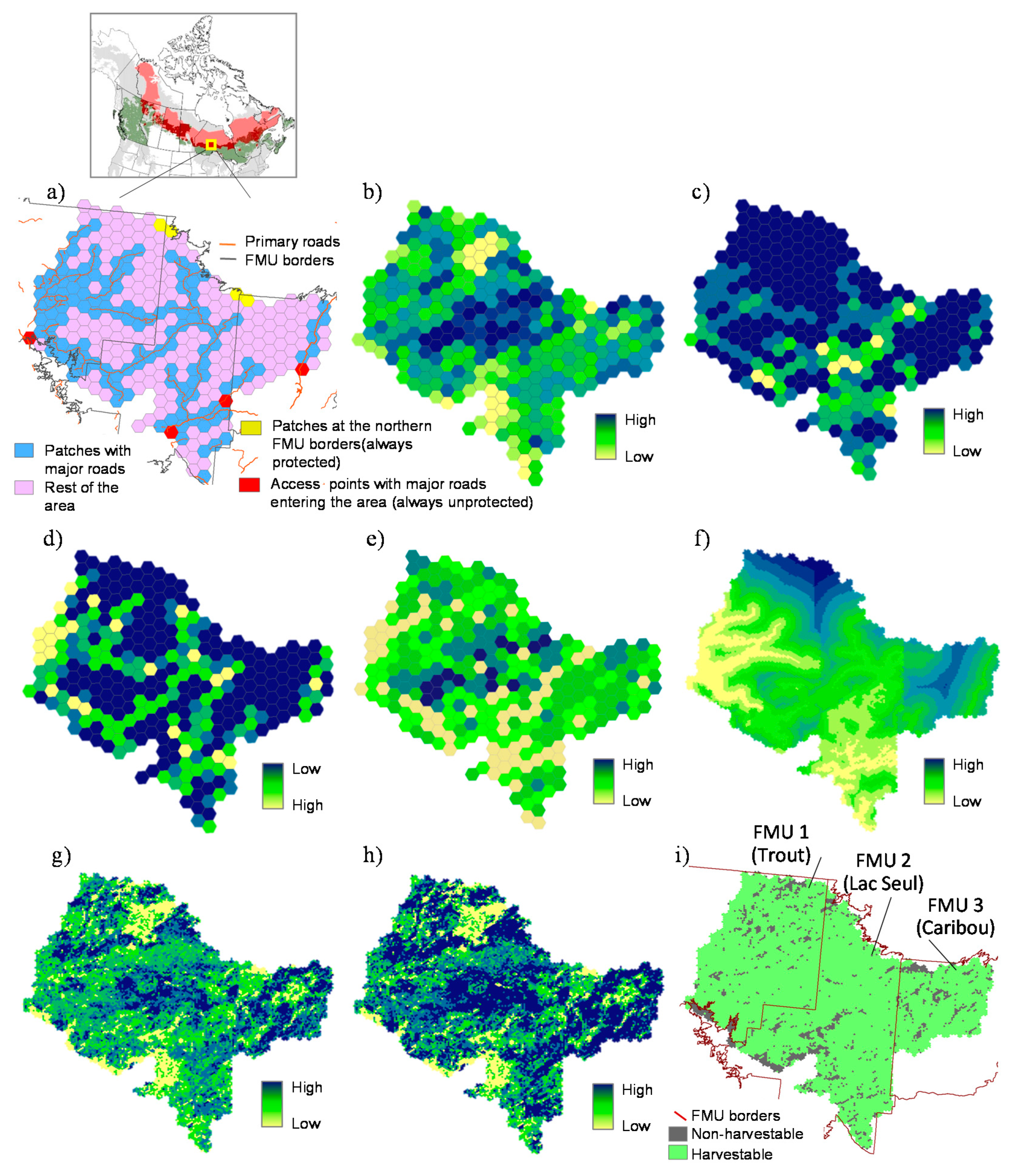
2.8. Case Study
2.9. Data
3. Results
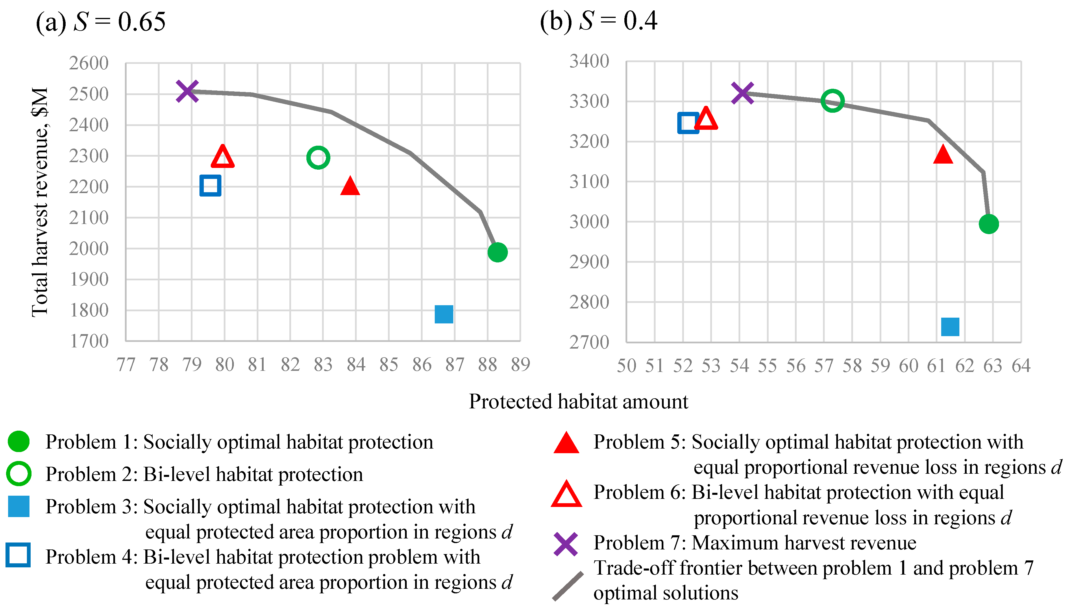
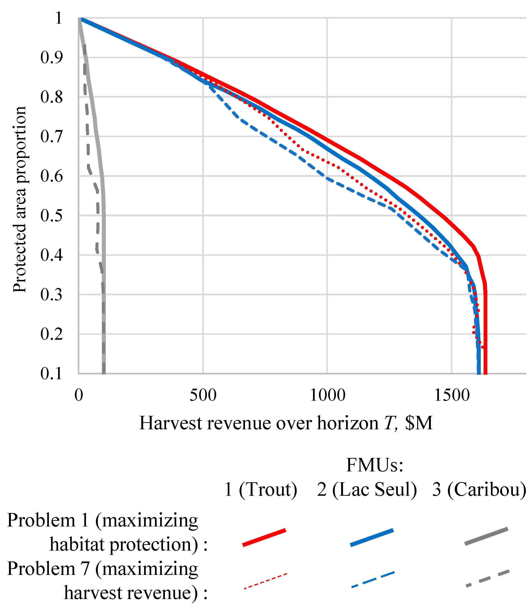
3.1. Trade-Off between Maximizing Habitat Protection and Maximizing Harvest Revenue
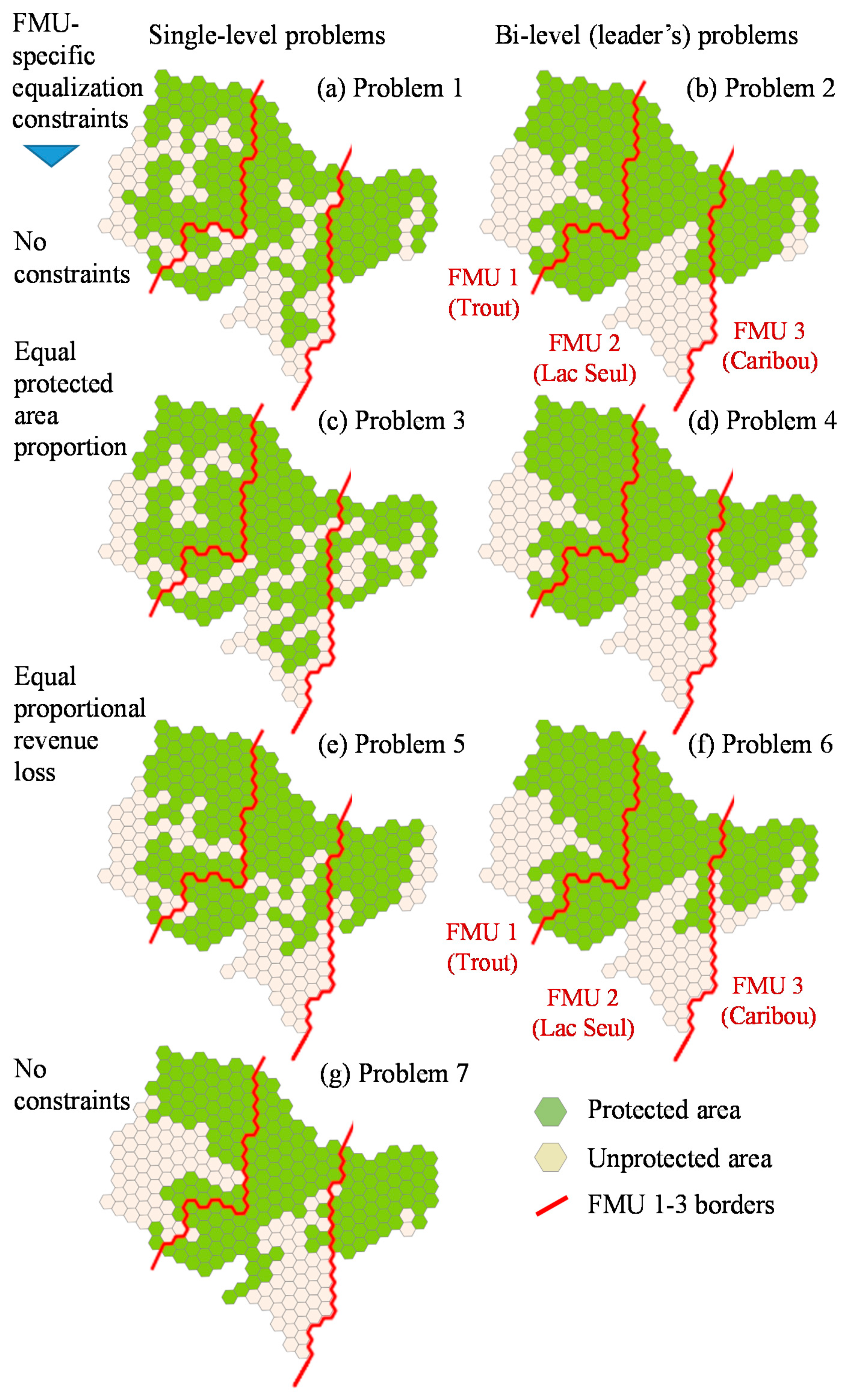
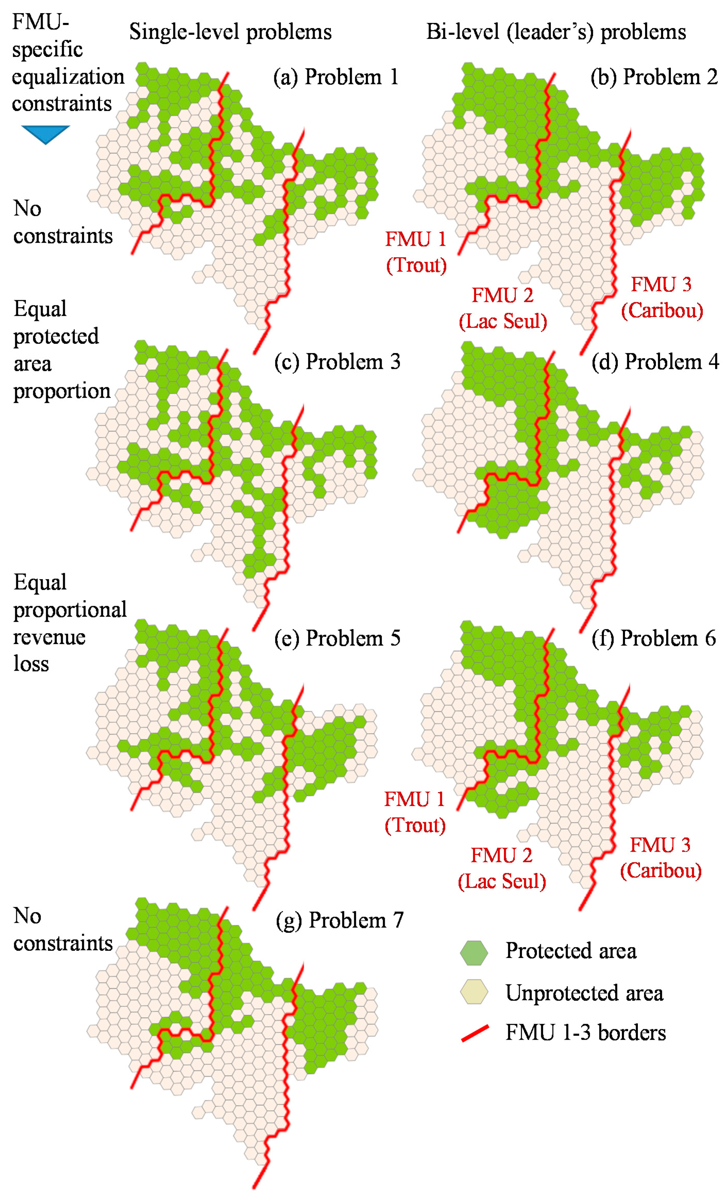
3.2. General Habitat Protection Patterns
4. Discussion
Author Contributions
Funding
Acknowledgments
Conflicts of Interest
References
- Brandt, J.P.; Flannigan, M.D.; Maynard, D.G.; Thompson, I.D.; Volney, W.J.A. An introduction to Canada’s boreal zone: Ecosystem processes, health, sustainability, and environmental issues. Environ. Rev. 2013, 21, 207–226. [Google Scholar] [CrossRef]
- Schaefer, J.A. Long-term range recession and the persistence of caribou in the taiga. Conserv. Biol. 2003, 17, 1435–1439. [Google Scholar] [CrossRef]
- Government of Canada. Species at Risk Act (SARA). Bill C-5, An Act Respecting the Protection of Wildlife Species at Risk in Canada. 25 August 2010. Available online: http://laws.justice.gc.ca/PDF/Statute/S/S-15.3.pdf (accessed on 2 February 2019).
- Festa-Bianchet, M.; Ray, J.C.; Boutin, S.; Cote, S.D.; Gunn, A. Conservation of caribou (Rangifer tarandus) in Canada: An uncertain future. Can. J. Zool. 2011, 89, 419–434. [Google Scholar] [CrossRef]
- Hebblewhite, M. Billion dollar boreal woodland caribou and the biodiversity impacts of the global oil and gas industry. Biol. Conserv. 2017, 206, 102–111. [Google Scholar] [CrossRef]
- Hebblewhite, M.; Fortin, D. Canada fails to protect its caribou. Science 2017, 358, 730–731. [Google Scholar] [PubMed]
- Environment Canada (EC). Recovery Strategy for the Woodland Caribou (Rangifer tarandus caribou), Boreal Population, in Canada; Species at Risk Act Recovery Strategy Series; Environment Canada: Ottawa, ON, Canada, 2012. Available online: http://www.registrelep-sararegistry.gc.ca/virtual_sara/files/plans/rs%5Fcaribou%5Fboreal%5Fcaribou%5F0912%5Fe1%2Epdf (accessed on 2 October 2019).
- Environment and Climate Change Canada (ECCC). Report on the Progress of Recovery Strategy Implementation for the Woodland Caribou (Rangifer tarandus caribou), Boreal Population in Canada for the Period 2012–2017; Species at Risk Act Recovery Strategy Series; Environment and Climate Change Canada: Ottawa, ON, Canada, 2017. Available online: http://registrelep-sararegistry.gc.ca/virtual_sara/files/Rs%2DReportOnImplementationBorealCaribou%2Dv00%2D2017Oct31%2DEng%2Epdf (accessed on 10 June 2020).
- Environment Canada (EC). Scientific Assessment to Support the Identification of Critical Habitat for Woodland Caribou (Rangifer tarandus caribou), Boreal Population, in Canada; Environment Canada: Ottawa, ON, Canada, 2011.
- McLoughlin, P.D.; Stewart, K.; Superbie, C.; Perry, T.; Tomchuk, P.; Greuel, R.; Singh, K.; Trucho-Savard, A.; Henkelman, J.; Johnston, J.F. Population Dynamics and Critical Habitat of Woodland caribou in the Saskatchewan Boreal Shield. Interim Project Report, 2013–2016; Department of Biology, University of Saskatchewan: Saskatoon, SK, Canada, 2016; Available online: http://mcloughlinlab.ca/lab/wp-content/uploads/2016/11/2013-2016-SK-Boreal-Shield-Caribou-Project-Interim-Report-Nov-18-2016.pdf (accessed on 22 December 2019).
- DeMars, C.A.; Boutin, S. Nowhere to hide: Effects of linear features on predator-prey dynamics in a large mammal system. J. Anim. Ecol. 2018, 87, 274–284. [Google Scholar] [CrossRef]
- Saher, D.J.; Schmiegelow, F.K.A. Movement pathways and habitat selection by woodland caribou during spring migration. Rangifer Spec. Issue 2005, 16, 143–154. [Google Scholar] [CrossRef]
- Ferguson, S.H.; Elkie, P.C. Seasonal movement patterns of woodland caribou (Rangifer tarandus caribou). J. Zool. 2004, 262, 125–134. [Google Scholar] [CrossRef]
- Redpath, S.M.; Gutiérrez, R.J.; Wood, K.A.; Young, J.C. (Eds.) Conflicts in Conservation: Navigating towards Solutions; Cambridge University Press: Cambridge, UK, 2015; 315p. [Google Scholar]
- Martin, A.B.; Ruppert, J.L.W.; Gunn, E.A.; Martell, D.L. A replanning approach for maximizing woodland caribou habitat alongside timber production. Can. J. For. Res. 2017, 47, 901–909. [Google Scholar] [CrossRef]
- McKenney, D.W.; Nippers, B.; Racey, G.; Davis, R. Trade-offs between wood supply and caribou habitat in northwestern Ontario. Rangifer 1997, 10, 149–156. [Google Scholar] [CrossRef][Green Version]
- McKenney, D.W.; Mussell, A.; Fox, G. An economic perspective on emulation forestry and a case study on woodland caribou-wood production trade-offs in northern Ontario. Chapter 17. In Emulating Natural Forest Landscape Disturbances: Concepts and Applications; Perera, A., Buse, L., Weber, M., Eds.; Columbia University Press: New York, NY, USA, 2004; pp. 209–218. [Google Scholar]
- Öhman, K.; Edenius, L.; Mikusiński, G. Optimizing spatial habitat suitability and timber revenue in long-term forest planning. Can. J. For. Res. 2011, 41, 543–551. [Google Scholar] [CrossRef]
- Ruppert, J.L.W.; Fortin, M.-J.; Gunn, E.A.; Martell, D.L. Conserving woodland caribou habitat while maintaining timber yield: A graph theory approach. Can. J. For. Res. 2016, 46, 914–923. [Google Scholar] [CrossRef]
- St. John, R.; Öhman, K.; Tóth, S.F.; Sandström, P.; Korosuo, A.; Eriksson, L.O. Combining spatiotemporal corridor design for reindeer migration with harvest scheduling in northern Sweden. Scand. J. For. Res. 2016, 37, 655–663. [Google Scholar] [CrossRef]
- St. John, R.; Tóth, S.F.; Zabinsky, Z. Optimizing the geometry of wildlife corridors in conservation reserve design. Oper. Res. 2018, 66. [Google Scholar] [CrossRef]
- Yemshanov, D.; Haight, R.G.; Koch, F.H.; Parisien, M.-A.; Swystun, T.; Barber, Q.; Burton, C.A.; Choudhury, S.; Liu, N. Prioritizing restoration of fragmented landscapes for wildlife conservation: A graph theoretic approach. Biol. Conserv. 2019, 232, 173–186. [Google Scholar] [CrossRef]
- Yemshanov, D.; Haight, R.G.; Liu, N.; Parisien, M.-A.; Barber, Q.; Koch, F.H.; Burton, C.; Mansuy, N.; Campioni, F.; Choudhury, S. Assessing the trade-offs between timber supply and wildlife protection goals in boreal landscapes. Can. J. For. Res. 2020, 50, 243–258. [Google Scholar] [CrossRef]
- Yemshanov, D.; Haight, R.G.; Rempel, R.; Liu, N.; Koch, F.H. Protecting wildlife habitat in managed forest landscapes-How can network connectivity models help? Nat. Resour. Model. 2020, e12286. [Google Scholar] [CrossRef]
- Conrad, J.; Gomes, C.P.; van Hoeve, W.-J.; Sabharwal, A.; Suter, J. Wildlife corridors as a connected subgraph problem. J. Environ. Econ. Manag. 2012, 63, 1–18. [Google Scholar] [CrossRef]
- Johnson, K.N.; Scheurman, H.L. Techniques for prescribing optimal timber harvest and investment under different objectives-discussion and synthesis. For. Sci. Monogr. 1977. [Google Scholar] [CrossRef]
- Boan, J.J.; Malcolm, J.R.; Vanier, M.D.; Euler, D.L.; Moola, F.M. From climate to caribou: How manufactured uncertainty is affecting wildlife management. Wildl. Soc. Bull. 2018, 42, 366–381. [Google Scholar] [CrossRef]
- Yenipazarli, A. Managing new and remanufactured products to mitigate environmental damage under emissions regulation. Eur. J. Oper. Res. 2016, 249, 117–130. [Google Scholar] [CrossRef]
- Gao, Y.; Li, Z.; Wang, F.; Wang, F.; Tan, R.R.; Bi, J.; Jia, X. A game theory approach for corporate environmental risk mitigation. Resour. Conserv. Recycl. 2018, 130, 240–247. [Google Scholar] [CrossRef]
- Karplus, V.J.; Zhang, S.; Almond, D. Quantifying coal power plant responses to tighter SO2 emissions standards in China. Proc. Natl. Acad. Sci. USA 2018, 115, 7004–7009. [Google Scholar] [CrossRef] [PubMed]
- Government of Ontario. Endangered Species Act, 2007, S.O. 2007, c. 6. Available online: https://www.ontario.ca/laws/statute/07e06 (accessed on 10 December 2020).
- Government of Ontario. Range Management Policy in Support of Woodland Caribou Conservation and Recovery. Available online: https://www.ontario.ca/page/range-management-policy-support-woodland-caribou-conservation-and-recovery (accessed on 2 March 2021).
- Myerson, R.B. Game Theory; Harvard University Press: Cambridge, MA, USA, 2013. [Google Scholar]
- Colson, B.; Marcotte, P.; Savard, G. An overview of bilevel optimization. Ann. Oper. Res. 2007, 153, 235–256. [Google Scholar] [CrossRef]
- Von Stackelberg, H. Market Structure and Equilibrium; Springer Science & Business Media: Berlin/Heidelberg, Germany, 2010. [Google Scholar]
- Paradis, G.; Bouchard, M.; LeBel, L.; D’Amours, S. Extending the Classical Wood Supply Model to Anticipate Industrial Fibre Consumption. Interuniversity Research Centre on Enterprise Network, Logistics and Transportation Report CIRRELT-2015-06. 2015. Available online: https://www.cirrelt.ca/documentstravail/cirrelt-2015-06.pdf (accessed on 1 October 2020).
- Paradis, G. Hierarchical Forest Management Planning. A Bilevel Wood Supply Modelling Approach. Ph.D. Thesis, University Laval, Québec, QC, Canada, 2016. Available online: https://corpus.ulaval.ca/jspui/bitstream/20.500.11794/27060/1/31750.pdf (accessed on 10 May 2020).
- Amacher, G.S.; Malik, A.S.; Haight, R.G. Reducing social losses from forest fires. Land Econ. 2006, 82, 367–383. [Google Scholar] [CrossRef][Green Version]
- Conitzer, V. On Stackelberg Mixed Strategies. Synthese 2016, 193, 689–703. [Google Scholar] [CrossRef]
- Colson, B.; Marcotte, P.; Savard, G. Bilevel programming: A survey. 4OR 2005, 3, 87–107. [Google Scholar] [CrossRef]
- Bard, J.F.; Plummer, J.; Sourie, J.C. A bilevel programming approach to determining tax credits for biofuel production. Eur. J. Oper. Res. 2000, 120, 30–46. [Google Scholar] [CrossRef]
- Brotcorne, L.; Labbé, M.; Marcotte, P.; Savard, G. A bilevel model for toll optimization on a multicommodity transportation network. Transp. Sci. 2001, 35, 345–358. [Google Scholar] [CrossRef]
- Burgard, A.P.; Pharkya, P.; Maranas, C.D. Optknock: A bilevel programming framework for identifying gene knockout strategies for microbial strain optimization. Biotechnol. Bioeng. 2003, 84, 647–657. [Google Scholar] [CrossRef]
- Ren, S.; Zeng, B.; Qian, X. Adaptive bi-level programming for optimal gene knockouts for targeted overproduction under phenotypic constraints. BMC Bioinform. 2013, 14, 1. Available online: https://bmcbioinformatics.biomedcentral.com/articles/10.1186/1471-2105-14-S2-S17 (accessed on 1 December 2020). [CrossRef]
- Raghunathan, A.U.; Biegler, L.T. Mathematical programs with equilibrium constraints (MPECs) in process engineering. Comput. Chem. Eng. 2003, 27, 1381–1392. [Google Scholar] [CrossRef]
- Raghunathan, A.U.; Diaz, M.S.; Biegler, L.T. An MPEC formulation for dynamic optimization of distillation operations. Comput. Chem. Eng. 2004, 28, 2037–2052. [Google Scholar] [CrossRef]
- Arroyo, J.M. Bilevel programming applied to power system vulnerability analysis under multiple contingencies. IET Gener. Transm. Distrib. 2010, 4, 178–190. [Google Scholar] [CrossRef]
- Hobbs, B.F.; Metzler, C.B.; Pang, J.-S. Strategic gaming analysis for electric power systems: An MPEC approach. IEEE Trans. Power Syst. 2000, 15, 638–645. [Google Scholar] [CrossRef]
- Hu, X.; Ralph, D. Using EPECs to model bilevel games in restructured electricity markets with locational prices. Oper. Res. 2007, 55, 809–827. [Google Scholar] [CrossRef]
- Bogle, T.; van Kooten, G.C. Why mountain pine beetle exacerbates a principal–agent relationship: Exploring strategic policy responses to beetle attack in a mixed species forest. Can. J. For. Res. 2012, 42, 621–630. [Google Scholar] [CrossRef]
- Ramo, J.; Tahvonen, O. Optimizing the harvest timing in continuous cover forestry. Environ. Resour. Econ. 2016, 67, 853–868. [Google Scholar] [CrossRef]
- Yue, D.; You, F. Game-theoretic modeling and optimization of multi-echelon supply chain design and operation under Stackelberg game and market equilibrium. Comput. Chem. Eng. 2014, 71, 347–361. [Google Scholar] [CrossRef]
- Zhai, W.; Zhao, Y.; Lian, X.; Yang, M.; Lu, F. Management planning of fast-growing plantations based on a bi-level programming model. For. Policy Econ. 2014, 38, 173–177. [Google Scholar] [CrossRef]
- Hornseth, M.L.; Rempel, R.S. Seasonal resource selection of woodland caribou (Rangifer tarandus caribou) across a gradient of anthropogenic disturbance. Can. J. Zool. 2015, 94, 79–93. [Google Scholar] [CrossRef]
- Johnson, C.J.; Parker, K.L.; Heard, D.C.; Gillingham, M.P. A multiscale behavioural approach to understanding the movements of woodland caribou. Ecol. Appl. 2002, 12, 1840–1860. [Google Scholar] [CrossRef]
- Rempel, R.S.; Hornseth, M.L. Range-Specific Seasonal Resource Selection Probability Functions for 13 Caribou Ranges in Northern Ontario; Science and Research Internal File Report IFR-01; Ontario Ministry of Natural Resources and Forestry, Science and Research Branch: Peterborough, ON, Canada, 2018; 42p.
- Rettie, W.J.; Messier, F. Range use and movement rates of woodland caribou in Saskatchewan. Can. J. Zool. 2001, 79, 1933–1940. [Google Scholar] [CrossRef]
- Sessions, J. Solving for habitat connections as a Steiner network problem. For. Sci. 1992, 38, 203–207. [Google Scholar]
- Jafari, N.; Hearne, J. A new method to solve the fully connected reserve network design problem. Eur. J. Oper. Res. 2013, 231, 202–209. [Google Scholar] [CrossRef]
- Keim, J.L.; Lele, S.R.; DeWitt, P.D.; Fitzpatrick, J.J.; Jenni, N.S. Estimating the intensity of use by interacting predators and prey using camera traps. J. Anim. Ecol. 2019, 88, 690–701. [Google Scholar] [CrossRef]
- Mumma, M.A.; Gillingham, M.P.; Johnson, C.J.; Parker, K.L. Understanding predation risk and individual variation in risk avoidance for threatened boreal caribou. Ecol. Evol. 2017, 7, 10266–10277. [Google Scholar] [CrossRef]
- National Forestry Database (NFD). Harvest. 5.2 Area Harvested by Jurisdiction, Tenure, Management and Harvesting Method. 2019. Available online: http://nfdp.ccfm.org/en/data/harvest.php (accessed on 17 May 2020).
- James, A.R.C.; Boutin, S.; Hebert, D.M.; Rippin, A.B. Spatial separation of caribou from moose and its relation to predation by wolves. J. Wildl. Manag. 2004, 68, 799–809. [Google Scholar] [CrossRef]
- Latham, A.D.M.; Latham, C.; McCutchen, N.A.; Boutin, S. Invading white-tailed deer change wolf-caribou dynamics in northeastern Alberta. J. Wildl. Manag. 2011, 75, 204–212. [Google Scholar] [CrossRef]
- Wittmer, H.U.; Sinclair, A.R.E.; McLellan, B.N. The role of predation in the decline and extirpation of woodland caribou. Oecologia 2005, 144, 257–267. [Google Scholar] [CrossRef]
- Ferguson, S.H.; Elkie, P.C. Habitat requirements of boreal forest caribou during the travel seasons. Basic Appl. Ecol. 2004, 5, 465–474. [Google Scholar] [CrossRef]
- Brown, G.S.; Mallory, F.F.; Rettie, J. Range size and seasonal movement for female woodland caribou in the boreal forest of northeastern Ontario. Rangifer 2003, 23, 227–233. [Google Scholar] [CrossRef][Green Version]
- Ontario Ministry of Natural Resources and Forestry (OMNRF). General Habitat Description for the Forest-Dwelling Woodland caribou (Rangifer tarandus caribou). 2015. Available online: http://govdocs.ourontario.ca/node/29324 (accessed on 1 February 2019).
- GAMS (GAMS Development Corporation). General Algebraic Modeling System (GAMS); Version 33; GAMS: Washington, DC, USA, 2020; Available online: http://www.gams.com (accessed on 1 April 2020).
- GUROBI (Gurobi Optimization Inc.). GUROBI Optimizer Reference Manual. Version 9.1. 2020. Available online: http://www.gurobi.com (accessed on 1 April 2020).
- Canadian Parks and Wilderness Society, Wildland League (CPAWS). A Snapshot of Caribou Range Condition in Ontario. Special Report. 2009. Available online: https://wildlandsleague.org/media/Caribou-Range-Condition-in-Ontario-WL2009-HIGH-RES.pdf (accessed on 13 October 2020).
- Ontario Ministry of Natural Resources (OMNR). Ontario’s Woodland Caribou Conservation Plan Progress Report Winter 2012; Ontario Ministry of Natural Resources: Toronto, ON, Canada, 2012. Available online: https://www.porcupineprospectors.com/wp-content/uploads/Woodland-Caribou.pdf (accessed on 1 February 2019).
- Elkie, P.; Green, K.; Racey, G.; Gluck, M.; Elliott, J.; Hooper, G.; Kushneriukand, R.; Rempel, R. Science and Information in Support of Policies that Address the Conservation of Woodland Caribou in Ontario: Occupancy, Habitat and Disturbance Models, Estimates of Natural Variation and Range Level Summaries. Electronic Document. Version 2018; Ontario Ministry of Natural Resources, Forests Branch: Toronto, ON, Canada, 2018.
- Natural Resources Canada (NRCan). Topographic Data of Canada-CanVec Series. 2019. Available online: https://open.canada.ca/data/en/dataset/8ba2aa2a-7bb9-4448-b4d7-f164409fe056 (accessed on 10 April 2020).
- Maure, J.; Ontario Forest Biofibre. Presentation Made at Cleantech Biofuels Workshop. 13 February 2013. Available online: https://www.sault-canada.com/en/aboutus/resources/Supporting_Doc_2_-_Available_biomass.pdf (accessed on 10 April 2019).
- Ontario Ministry of Natural Resources and Forestry (OMNRF) Forest Resources Inventory (FIM v 2.2D) Packaged Product. 2019. Available online: https://geohub.lio.gov.on.ca/datasets/forest-resources-inventory-fim-v2-2d-packaged-product (accessed on 1 February 2019).
- McKenney, D.W.; Yemshanov, D.; Pedlar, J.; Allen, D.; Lawrence, K.; Hope, E.; Lu, B.; Eddy, B. Canada’s Timber Supply: Current Status and Future Prospects under a Changing Climate; Information Report GLC-X-15; Natural Resources Canada, Canadian Forest Service, Great Lakes Forestry Centre: Sault Ste. Marie, ON, Canada, 2016. [Google Scholar]
- Boulanger, Y.; Gauthier, S.; Burton, P.J. A refinement of models projecting future Canadian fire regimes using homogeneous fire regime zones. Can. J. For. Res. 2014, 44, 365–376. [Google Scholar] [CrossRef]
- Ontario Nature. How Can We Protect Critical Caribou Habitat and Support Forestry Jobs in Ontario? A Background Paper Prepared by Ontario Nature. June 2019. Available online: https://davidsuzuki.org/wp-content/uploads/2019/06/how-can-we-protect-critical-caribou-habitat-and-support-forestry-jobs-in-ontario-2.pdf (accessed on 10 January 2021).
- Bentham, P.; Coupal, B. Habitat restoration as a key conservation lever for woodland caribou: A review of restoration programs and key learnings from Alberta. Rangifer Spec. Issue 2015, 35, 123–148. [Google Scholar] [CrossRef]
- Forest Stewardship Council (FSC) Canada Working Group. National Boreal Standard. 6 August 2004. Available online: https://ca.fsc.org/preview.national-boreal-standard.a-822.pdf (accessed on 10 January 2021).
- Forest Stewardship Council (FSC) Canada. FSC National Forest Stewardship Standard of Canada. 2018. Available online: https://ca.fsc.org/download.fsc-std-can-01-2018-en-v1.a-2364.pdf (accessed on 10 December 2020).
- Dzus, E.; Ray, J.; Thompson, I.; Wedeles, C. Caribou and the National Boreal Standard: Report of the FSC Canada Science Panel, Prepared for FSC Canada. 26 July 2010. Available online: https://ca.fsc.org/preview.caribou-and-the-national-boreal-standard-report-of-the-fsc-canada-science-panel.a-498.pdf (accessed on 10 January 2021).
- Crown Forest Sustainability Act., S.O. 1994, c.25. 1994. Available online: https://www.ontario.ca/laws/statute/94c25 (accessed on 1 December 2020).


| Symbol | Parameter/Variable Name | Description |
|---|---|---|
| Sets: | ||
| J | Patches j, k with suitable habitat—potential candidates for protection in a landscape J | j,k ∊ J |
| Jd | Patches j, k with suitable habitat located in region d | Jd ∊ J |
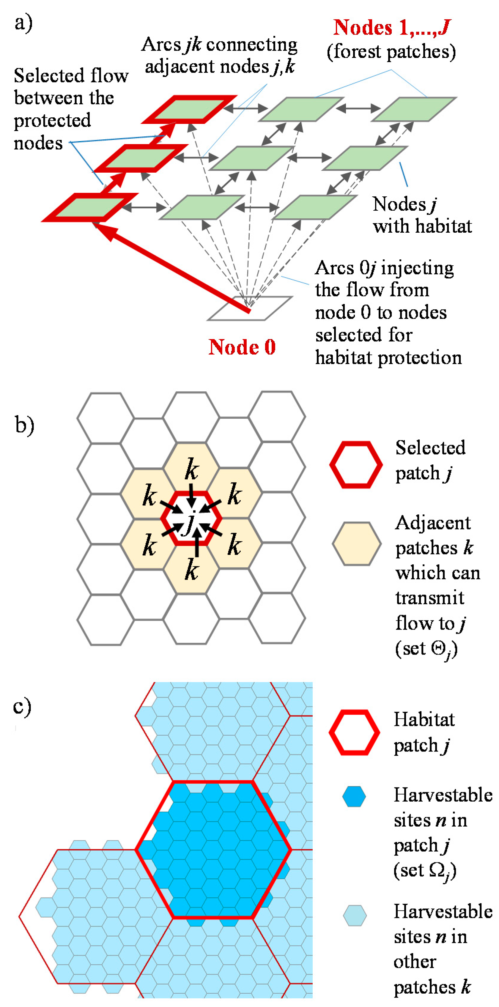
| Θj | Patches k which are connected to patch j and can transmit flow to j | kj ∊ Θj |
| Θj+ | Patches k which are connected to patch j and can receive flow from j | kj ∊ Θj |
| Θ jd | Patches k located in region d which can transmit flow to patch j located in region d | Θjd ∊ J |
| N | Forest sites n—potential harvest blocks in landscape N | n ∊ N |
| Nd | Forest sites n—potential harvest blocks located in region d | Nd ∊ N |
| Ωj | Forest sites n—potential harvest blocks located in habitat patch j | Ωj ∊ N |
| D | Forest management regions d where individual players (the followers) operate | d ∊ D |
| C | Habitat protection levels c | c ∊ C |
| T | Planning time periods, t | t ∊ T |
| I | Harvest prescriptions, i | i ∊ I |
| Decision variables: | ||
| wkj | Binary indicator of the species flow via arc kj in the protected area over timespan T | wjk ∊ {0,1} |
| vkj | Binary indicator of the connection between the adjacent unprotected patches k and j | vjk ∊ {0,1} |
| ykj | Amount of flow between the adjacent protected patches k and j | yjk ≥ 0 |
| zkj | Amount of flow between the adjacent unprotected patches k and j | zjk ≥ 0 |
| xni | Binary selection of harvest prescription i in site n | xni ∊ {0,1} |
| ωdc | Binary selection of the follower’s optima from a solution set for D regions × C protection levels | ωdc ∊ {0,1} |
| The value of binary variable ωdc denoting the selection of the precomputed follower’s solution c with the protected area portion of FMU d equal to selected target S. | ∊{0,1} | |
| P1 | The number of connections to node 0 above one in the network of protected patches | P1≥ 0 |
| P2 | The number of connections to node 0 above θ in the network of unprotected patches | P2≥ 0 |
| G | Proportional harvest revenue loss in region d over timespan T under protection level c | G ≥ 0 |
| Qd | Maximum sustainable harvest volume in region d in period t | Qd ≥ 0 |
| Parameters | ||
| bnit | Habitat amount in site n in prescription i in period t | bnit ≥ 0 |
| βnit | Habitat suitability in site n in prescription i in period t | βnit ≥ 0 |
| Bj | Habitat amount in patch j under protection (assuming the no-harvest prescription i = 1) | Bj ≥ 0 |
| αn | Habitat area in site n | αn ≥ 0 |
| Aj | Habitat area in patch j | Aj ≥ 0 |
| an | Harvestable forest area in site n | an ≥ 0 |
| Vnit | Volume of timber available for the harvest at site n in period t in prescription i | Vnit ≥ 0 |
| Rni | Net cash flow associated with harvesting site n according to prescription i | Rni ≥ 0 |
| ETmin | Average target forest age in the managed area at the end of the planning horizon T | 80 |
| Eni | Forest stand age in site n at the end of the planning horizon if prescription i is applied | 0–250 |
| ρn | Net unit price of timber harvested from site n | ρn > 0 |
| en | Postharvest regeneration costs | en > 0 |
| Sd | Target proportion of the protected area in region (FMU) d | Sd ∊ [0;1] |
| Sc | Target proportion of the protected area at protection level c | Sc ∊ [0;1] |
| S | Target proportion of the protected range area | S ∊ [0;1] |
| χjdc | Binary selection of patch j for protection in the follower’s solution for region d protection level c | χjdc ∊ {0,1} |
| rmax d | Harvest revenue in the maximum sustainable harvest scenario without protection in region d | rmax d ≥ 0 |
| rdc | Total harvest revenue over horizon T in region d at protection level c | rdc ≥ 0 |
| gdc | Proportional loss in harvest revenue in region d at protection level c vs. no-protection scenario | gdc ∊ [0;1] |
| ψj | Binary indicator of patches in northwestern and northeastern region’s corners which must remain unharvested to maintain the connectivity of habitat between regions | ψj ∊ {0,1} |
| γjd | Binary parameter defining patches j located in region d | γjd ∊ {0,1} |
| δnd | Binary parameter defining sites n located in region d | δnd ∊ {0,1} |
| μj | Binary parameter defining sites where permanent roads enter the area | μj ∊ {0,1} |
| θ | The number of major access points of entry to the range area (equal to the number of regions D) | 3 |
| σ | Allowable decrease in harvest volume in consecutive planning periods t and t +1 | 0.02 |
| ε | Small value | 0.05 |
| f1, f2, f3 | Scaling factors | f1, f2, f3 > 0 |
| U | Large positive value | U > 0 |
| Problem Type and Objective | Equalization Constraints for FMUs d | ||
|---|---|---|---|
| None | Equal Protected Area Proportion | Equal Proportional Harvest Revenue Loss | |
| Bi-level, max (protected habitat) | Bi-level habitat protection problem 2 | Bi-level equal protected area proportion problem 4 | Bi-level equal proportional revenue loss problem 6 |
| Single-level, socially optimal max (protected habitat) | Socially optimal habitat protection problem 1 | Socially optimal habitat protection equal protected area proportion problem 3 | Socially optimal habitat protection equal proportional revenue loss problem 5 |
| Single-level, max (harvest revenue) | Maximum harvest revenue problem 7 | ||
| Land Cover Type | Habitat Type | ||
|---|---|---|---|
| Useable | Preferred | Refuge | |
| Lowland spruce | 61 | ||
| Mixedwood conifers | 71 | ||
| Other lowland conifers | 51 | 41 * | |
| Jack pine dominant | 41 | 61 | 41 * |
| Jack pine mixed wood | 41 | 61 | 41 |
| Black spruce dominant or black spruce mixed wood | 61 | 41 | |
| Black spruce lowland | 41 | 101 | 41 * |
| Treed bog and fen | Permanent | Permanent | |
| Problem | Protected Habitat Amount | Total Harvest Revenue | Protected Area Proportion Target | Actual Protected Area Proportion | Protected Area Proportion per Region | Harvest Revenue Loss Ratio per Region * | ||||||
|---|---|---|---|---|---|---|---|---|---|---|---|---|
| FMU 1 Trout | FMU 2 Lac Seul | FMU 3 Caribou | Min-Max Range | FMU 1 Trout | FMU 2 Lac Seul | FMU 3 Caribou | Min-Max Range | |||||
| Protected area proportion target S = 0.65 | ||||||||||||
| Problem 1: Socially optimal habitat protection | 88.3 | 1987.4 | 0.65 | 0.67 | 0.668 | 0.596 | 0.909 | 0.313 | 0.457 | 0.335 | 0.715 | 0.38 |
| Problem 2: Bi-level habitat protection | 82.9 | 2294 | 0.65 | 0.67 | 0.632 | 0.631 | 0.89 | 0.259 | 0.289 | 0.317 | 0.694 | 0.405 |
| Problem 3: Socially optimal habitat protection with equal protected area % in FMUs d | 86.7 | 1786.9 | 0.65 | 0.67 | 0.674 | 0.675 | 0.673 | 0.002 | 0.469 | 0.463 | 0.477 | 0.014 |
| Problem 4: Bi-level habitat protection problem with equal protected area % in FMUs d | 79.6 | 2203.7 | 0.65 | 0.66 | 0.655 | 0.655 | 0.654 | 0.001 | 0.33 | 0.364 | 0.172 | 0.192 |
| Problem 5: Socially optimal habitat protection with equal proportional revenue loss in FMUs d | 83.8 | 2205.1 | 0.65 | 0.66 | 0.655 | 0.621 | 0.749 | 0.128 | 0.345 | 0.338 | 0.338 | 0.007 |
| Problem 6: Bi-level habitat protection with equal proportional revenue loss in FMUs d | 79.9 | 2300 | 0.65 | 0.65 | 0.644 | 0.631 | 0.729 | 0.098 | 0.308 | 0.317 | 0.317 | 0.009 |
| Problem 7: Maximum harvest revenue | 78.9 | 2509.3 | 0.65 | 0.64 | 0.51 | 0.65 | 0.948 | 0.438 | 0.111 | 0.353 | 0.884 | 0.773 |
| Protected area proportion target S = 0.4 | ||||||||||||
| Problem 1: Socially optimal habitat protection | 62.9 | 2993.9 | 0.4 | 0.42 | 0.478 | 0.294 | 0.6 | 0.31 | 0.224 | 0.004 | 0.336 | 0.34 |
| Problem 2: Bi-level habitat protection | 57.3 | 3308.6 | 0.4 | 0.42 | 0.494 | 0.248 | 0.691 | 0.44 | 0.101 | 0.005 | 0.227 | 0.23 |
| Problem 3: Socially optimal habitat protection with equal protected area % in FMUs d | 61.5 | 2737.9 | 0.4 | 0.41 | 0.414 | 0.415 | 0.409 | 0.01 | 0.202 | 0.165 | 0.132 | 0.07 |
| Problem 4: Bi-level habitat protection problem with equal protected area % in FMUs d | 52.2 | 3245.6 | 0.4 | 0.40 | 0.397 | 0.397 | 0.404 | 0.01 | 0.012 | 0.051 | 0.001 | 0.05 |
| Problem 5: Socially optimal habitat protection with equal proportional revenue loss in FMUs d | 61.2 | 3170 | 0.4 | 0.41 | 0.429 | 0.341 | 0.586 | 0.25 | 0.086 | 0.005 | 0.27 | 0.27 |
| Problem 6: Bi-level habitat protection with equal proportional revenue loss in FMUs d | 52.8 | 3259 | 0.4 | 0.40 | 0.397 | 0.4 | 0.421 | 0.02 | 0.013 | 0.042 | 0.001 | 0.04 |
| Problem 7: Maximum harvest revenue | 54.1 | 3320.5 | 0.4 | 0.40 | 0.384 | 0.311 | 0.661 | 0.35 | 0.002 | 0.007 | 0.133 | 0.13 |
Publisher’s Note: MDPI stays neutral with regard to jurisdictional claims in published maps and institutional affiliations. |
© 2021 by the authors. Licensee MDPI, Basel, Switzerland. This article is an open access article distributed under the terms and conditions of the Creative Commons Attribution (CC BY) license (https://creativecommons.org/licenses/by/4.0/).
Share and Cite
Yemshanov, D.; Haight, R.G.; Liu, N.; Rempel, R.S.; Koch, F.H.; Rodgers, A. Balancing Large-Scale Wildlife Protection and Forest Management Goals with a Game-Theoretic Approach. Forests 2021, 12, 809. https://doi.org/10.3390/f12060809
Yemshanov D, Haight RG, Liu N, Rempel RS, Koch FH, Rodgers A. Balancing Large-Scale Wildlife Protection and Forest Management Goals with a Game-Theoretic Approach. Forests. 2021; 12(6):809. https://doi.org/10.3390/f12060809
Chicago/Turabian StyleYemshanov, Denys, Robert G. Haight, Ning Liu, Robert S. Rempel, Frank H. Koch, and Art Rodgers. 2021. "Balancing Large-Scale Wildlife Protection and Forest Management Goals with a Game-Theoretic Approach" Forests 12, no. 6: 809. https://doi.org/10.3390/f12060809
APA StyleYemshanov, D., Haight, R. G., Liu, N., Rempel, R. S., Koch, F. H., & Rodgers, A. (2021). Balancing Large-Scale Wildlife Protection and Forest Management Goals with a Game-Theoretic Approach. Forests, 12(6), 809. https://doi.org/10.3390/f12060809