Modeling and Optimization Sustainable Forest Supply Chain Considering Discount in Transportation System and Supplier Selection under Uncertainty

Abstract

In recent decades, the forest industry has been growingly expanded due to economic conditions, climate changes, environmental and energy policies, and intense demand changes. Thus, appropriate planning is required to improve this industry. To achieve economic, social and environmental goals, a supply chain network is designed based on a multi-period and multi-product Mixed-Integer Non-Linear Programming (MINLP) model in which the objective is to maximize the profit, minimize detrimental environmental effects, improve social effects, and minimize the number of lost demands. In addition, to improve forest industry planning, strategic and tactical decisions have been implemented throughout the supply chain for all facilities, suppliers and machinery. These decisions significantly help to improve processes and product flows and to meet customers’ needs. In addition, because of the presence of uncertainty in some parameters, the proposed model was formulated and optimized under uncertainty using the hybrid robust possibilistic programming (HRPP-II) approach. The $\epsilon$-constraint technique was used to solve the multi-objective model, and the Lagrangian relaxation (LR) method was utilized to solve the model of more complex dimensions. A case study in Northern Iran was conducted to assess the efficiency of the suggested approach. Finally, a sensitivity analysis was performed to determine the impact of important parameters on objective functions. The results of this study show that increasing the working hours of machines instead of increasing their number, increasing the capacity of some facilities instead of establishing new facilities and expanding the transport fleet has a significant impact on achieving predetermined goals.

1. Introduction

Over recent decades, the demand for forestry products has risen around the world so that the development of the forest industry is not unexpectable. The forest industry contributes to 2–3% of the world GDP, whose annual value is estimated at USD 1,600,000 million. Nevertheless, this industry has been growing recently due to the economic conditions, climate changes, environmental and energy policies, and intense demand changes [1].

The concept of the supply chain (SC) can effectively help in planning and decision making in complex industries. A supply chain comprises centers, installations, and facilities helping the production of raw materials and various goods and product distribution in customers’ regions. Similarly to any other supply chain, forest supply chains also include these organizations. A forest supply chain consists of various production stages, processes, flows, and different products. Processes such as harvesting, distribution, transportation, and products such as biomass, energy, ethanol, wood, paper, and medium-density fiber (MDF) boards form the main body of these chains [2].

Such a supply chain is considered a complex one since it comprises several independent units, each responsible for a large number of dependent activities [3]. Thus, the use of supply chain techniques and logistics has increasingly been important regarding the forest industry [4,5]. A forest supply chain includes two main aspects, namely, forestry and forest management (such as planting, harvesting, transportation.) and production and industrial operations (e.g., producing lumbers, ethanol, energy) [6].

In addition, integrating and coordinating strategic, tactical, and operational decisions is vital to supply chain planning. Given the complex and large-scale problems, along with the diversity of products, suppliers, demand centers, periods, and operational, production, and logistic processes, it is usually necessary to use decomposition techniques and/or hierarchical planning methods [7]. Strategic decisions create limitations in the tactical planning process, which in turn cause barriers to the operational planning process [8]. Therefore, the forestry management community believes that a hierarchy of decisions at three levels, i.e., strategic, tactical, and operational levels, is an appropriate planning approach in this industry [1]. Accordingly, in this study, three strategic, tactical and operational planning approaches were implemented throughout the forest supply chain to help make better and more effective decisions.

The transportation of logs, wood residues, and chips, as raw materials, as well as the overall transportation system, contribute to 45% of the total costs of this industry. Consequently, strategic, tactical, and operational decisions, in terms of forest supply chain transportation systems, are of great importance [9,10]. At the strategic level, decisions are mainly related to road investments, facility location, and transportation system management [4,11]. The tactical decisions address planning the allocation of products from harvesting sites to production facilities [12,13]. Moreover, the decisions of the operational level are concerned with the routing and scheduling of machinery and equipment. To investigate the impact of the transport fleet and the number of vehicles and their rental costs on the forest supply chain, a discount model on the number of transport fleets was used.

Another notable decision-making level in the forest supply chain is inventory control and planning that accounts for 40% of the annual costs of this industry under supply and demand uncertainty [14,15]. Therefore, an inventory management system requires coordinated inventory decisions at each level and in each facility of the supply chain. In the model presented in this research, the inventory level for all supply chain facilities is considered in order to minimize the costs of maintaining production by adopting the best inventory level for each facility.

The forest industry plays a significant role in the social and economic development of many countries, as some regions and populations are involved in and affected by this industry [2]. An important concept that should be taken into consideration in supply chain design is the sustainability approach with the main components being the economic, environmental, and social dimensions [16,17]. Eskandarpour et al. [18] emphasized that only a few cases out of numerous investigations on the supply chain design have referred to sustainable development as a remarkable feature of this issue… Many studies have been affected by the economic dimension and somewhat by the environmental vision, while the social aspect of this industry has less been regarded [19,20]. This fact has been concluded by some investigations such as a quantitative assessment of relevant articles [21]. In order to evaluate all three dimensions of supply chain management in the forest industry, the goals of profit maximization, reduction in environmental pollutants and maximization of employment rate and reduction in unemployment rate are included in this research.

Regarding the above discussions, this research aims to present an optimization model for a forest supply chain network to not only focus on diverse products, but also plan on harvesting raw materials required for production centers. In addition, various tactical, strategic, and operational decisions, as well as sustainability aspects in the transportation system are considered in the model, Further, regarding the uncertainty of some variables in the real world, we design and optimize the proposed model under uncertainty to present a more realistic and efficient model to decision makers.

2. Literature Review

The forest supply chain comprises different levels, including production facilities, inventory control for a variety of products, and the transportation system, whose planning requires the use of tactical, strategic, and operational decisions.

2.1. Sustainable Forest Supply Chain

When it arose, the concept of forest industry sustainability had no clear focus on forest wood production and supply. Later, this concept was developed, and already it involves three dimensions, i.e., economic, environmental, and social, in all parts of the forest supply chain [22]. A review by [23] on research related to forest supply chains from 1995 to 2017, shows that almost 85% of studies have only focused on economic and environmental dimensions or a combination of the two. Although the social dimension has less been regarded, this aspect of sustainability greatly affects society, customer satisfaction, and the social environment in which the industry is active. For example, establishing a new industry in a region can improve living conditions, employment, and development rate [23]. Already, multi-objective optimizations are used extensively for integrating social or environmental dimensions with the economic aspect. Economic objective functions are often regarded as minimizing the total network cost [24,25] or maximizing the profit [26,27]. Environmental objectives are also incorporated into the model using various criteria, such as the Eco-indicator 99, IMPACT 2002+, and carbon footprint. Minimizing greenhouse gas emissions in the product life-cycle via the life-cycle assessment (LCA) is the most frequently used approach [28,29]. On the other hand, the social objective function tries to improve the efficiency of supply chain networks by increasing job capacity, decreasing the unemployment rate, and improving working conditions. Some studies have merely considered the economic dimension of the forest supply chain in order to be able to reduce sustainability costs and increase effectiveness [30,31,32]. In addition, Machani et al. [33] focused on the optimization of the net present value, and the authors of [34,35] attempted to improve the economic aspect of the forest supply chain by maximizing harvesting volume and demand satisfaction. Mobini et al. [36] regarded the minimization of costs and CO₂ emissions to address two sustainability aspects in the forest supply chain. Handler et al. [37] investigated the harvest and transportation processes in a wood supply chain to assess the consequences of fossil energy demand and environmental pollution. Boukherroub et al. [38] developed a mathematical model for a lumber supply chain in Canada, including economic, social, and environmental objectives. They solved the model using a weighted goals programming approach. Some other studies, sought to minimize detrimental environmental effects along with adopting strategic decisions [39,40,41,42,43,44]. The first one developed an optimization model to evaluate GHG and GWP emissions. The second determined the optimal amount of biomass to be supplied for power stations by minimizing global warming. The third one also tried to determine the optimal uses of biomass resources concerning global warming minimization. Chazara et al. [40] proposed a model to the optimal design of a bio-ethanol supply chain considering the number of jobs created by this industry. Leong et al. [41] suggested a sustainable bioenergy supply chain network considering CO₂ minimization. Meyer et al. [2] presented a multi-objective optimization problem for a sustainable forest supply chain, aiming at minimizing the costs and environmental impacts and maximizing social effects. She et al. [42,43,44] formulated two multi-period multi-product models for the forest supply chain considering economic and environmental aspects. H. Woo et al. [45] proposed a GIS-based model for lumber production, including all three sustainability elements.

2.2. Forest Supply Chain Planning and Decision-Making

As awareness of sustainability in supply chains, particularly forestry, increased, research on this concept has grown continuously [2,14,46,47]. However, due to the increased complexity caused by including sustainability, researchers attempted to use quantitative techniques such as mathematical modeling and optimization [9,48,49,50]; although decision-making approaches such as multi-criteria decision analysis (MCDA) and life cycle assessment (LCA) can also be used in this area, the most frequently used decision-making approach regarding the economic, social, and environmental dimensions of the supply chain is the mathematical programming, i.e., optimization [51]. Now, studies conducted on strategic, tactical, and operational decision making using optimization were reviewed.

Gunnarsson et al. [52] presented a mathematical model to find the optimal amount of raw material transportation from forest to pulp mills. Beaudoin et al. [53] formulated a Monte Carlo-based mixed integer programming (MIP) model to maximize the revenue obtained from the sale of wood and wood chips with respect to transportation costs. Lòpez et al. [54] developed a MIP model to minimize wood pulp supply chain costs. Additionally, Chauhan et al. [55] formulated a lumber supply chain to obtain optimal transportation costs. Kanzian et al. [56] examined an MIP and an LP model for a biomass supply chain and concluded that the direct transportation of wood and chippings at harvesting sites was cheaper than establishing separate terminals. Galatsidas et al. [34] presented two MIP models to optimize strategic decisions on production and oak harvest scheduling. Rix et al. [57] also proposed an MIP model in which, besides minimizing transportation costs, a penalty was considered for unsatisfied demands. Sacchelli et al. [27] incorporated economic, social, and environmental features of a supply chain into the production of biomass energy. Akhtari et al. [58] established an LP model for a biomass supply chain to decide the optimal amount of wood chips transport, inventory, and production. Gautam et al. [59] proposed a simulation–optimization model for tactical and operational decisions on harvest scheduling, in which the harvesting quantity was optimized in each period under demand constraints. Santibañez-Aguilar et al. [35] also designed a model to determine the technology, production facilities, and raw material flow. The model involved two objectives, aiming at maximizing demand satisfaction and increasing profit from the wood supply chain. Sosa et al. [60] formulated an LP model to determine the costs of harvesting, chipping, transportation, and storage in a wood biomass supply chain. Boukherroub et al. [38] built a three-objective model to optimize a lumber supply chain in Canada, aiming at reducing costs and greenhouse gas emissions and increasing the associated employment. Oliveira et al. [61] proposed an information system to optimize raw material utilization in the production system, focusing on strategic decisions. Palander [62] assessed the effects of different transportation and vehicle capacity scenarios in the forest industry on CO₂ emission. The results indicated that increasing the vehicle capacity caused CO₂ emission to decrease. Campanella et al. [6] developed a single-objective single-period MILP model to design a forest supply chain optimally in order to decide on establishing facilities with a specific capacity. Their model dealt with supplying raw materials for some products such as wood, wood chips, and energy in wood harvesting sites. Most of the relevant optimization approaches considered were bioenergy production [63], bioproduct [64], or both [65]. Other studies have merely regarded one product, such as wood [61] or paper [33]. In other words, these works focused on a particular product. Whitman et al. [66] studied the optimization of wood product transportation. Campanella et al. [6] presented a single-objective single-period MILP mathematic model for the forest supply chain in order to obtain the optimal facility location, the amounts of products, and all the material flows between forest sites. Most of the work on certain and uncertain programming has included stochastic programming, robust programming, robust optimization, and fuzzy programming [67]. She et al. [44] presented a bi-objective MILP model for a forest supply chain with economic and environmental approaches to mitigate detrimental environmental effects while minimizing costs. They used the $\epsilon$-constraint method to solve the model. Jonkman et al. [68,69] designed a single-period bi-objective model for a biomass supply chain considering economic and environmental dimensions. In addition, their model included strategic and operational planning for determining the optimal harvesting amount and transportation and location of biorefinery facilities. Meyer et al. [2] presented a multi-objective multi-product and single-period MILP model to design a sustainable forest supply chain optimally. The model allowed them to carry out strategic and operational planning for facility location, transportation volume, and wood residue harvesting volume. In addition, their model considered byproducts of each facility as raw material for other facilities. They solved the model using the $\epsilon$-constraint technique. Woo et al. [45] developed a GIS-based optimization model for lumber production dealing with the facility location problem in the forest industry in order to create a balance between economic, social, and environmental dimensions. They found that a major part of the cost was related to transporting forest resources to facilities. She et al. [42] formulated a metaheuristic solution approach to optimize a multi-period multi-product MIP model for a forest supply chain by minimizing costs and environmental pollutions. Moreover, the optimal amount of wood and wood residue harvesting and the produced pellet amount were determined. Fernandez-Lacruz et al. [70] developed a simulation-based costs analysis for wood chips production from logging residues. Already, one of the popular techniques in this industry is the maximum utilization of truck payload [71].

2.3. Research Gap, Goals and Assumptions

Prior research was mostly confined to one wood product, such as lumber, bioenergy, ethanol, or biomass. Therefore, aggregating all these items has not been previously addressed [43]. For this purpose, providing a model to plan for and decide on several products in a forest supply chain can remarkably help to understand this industry and improve its performance. The cost of the forest supply chain highly depends on the transport of resources, raw materials, and products within the chain [70]. Planning for reducing transportation costs according to real-world situations helps to solve this problem significantly. Specifically, some decisions can be determined on the number of vehicles, their capacity, and the number of their travels [72]. Another less-addressed issue is the constraints existing in the forest supply chain, including harvesting constraints, transportation constraints, the maximum number of transportation fleets, and machinery constraints [58,66]. Inventory control is also a valuable technique in reducing pollution, costs, and the number of travels [73]. Currently, a few studies have directly dealt with all three aspects of forest supply chain sustainability. Therefore, incorporating economic, social, and environmental considerations simultaneously into the forest supply chain is highly important [2]. Uncertainty plays a notable role in supply chain decision making. Uncertain parameters, robust optimization, and fuzzy uncertainty are some appropriate techniques that help to handle uncertainty in the forest supply chain [74,75,76,77]. In addition, the balance between costs, customer demand satisfaction and environmental effects will be key factors in the supply chain [78,79].

Regarding the above discussions, we intend to design a sustainable forest supply chain focusing on strategic, tactical, and operational decisions and economic, social, and environmental aspects of sustainability to fill the existing gap. This paper pursues the following goals.

• Developing a mathematical model for a sustainable forest supply chain to deal with multiple products;
• Improving the adverse impacts of transportation costs;
• Making more deliberate and realistic strategic, tactical, and operational decisions;
• Investigating the impact of uncertainty on forest supply chain models.

According to the literature review, this research developed a multi-objective multi-product multi-period MINLP model for a sustainable forest supply chain under uncertainty, particularly for strategic, tactical, and operational decision making. To improve the sustainability of the model, we incorporated four objective functions into the model, namely, maximizing the profit; minimizing environmental impacts of harvesting, production, and transportation; improving social dimensions considering the number of jobs created, development rate of regions, and suppliers; minimizing lost demand.

As stated before, a few studies incorporate uncertainty into this industry, causing the proposed models not to be in accord with real-world situations and decisions not to be documentable. This paper intends to incorporate uncertainty into the model. For this purpose, uncertainty is seen in some input parameters, and a robust fuzzy approach was used to deal with it.

Regarding all these gaps reviewed, the present research aims to cover these neglected concepts in the forest supply chain. In what follows, some important innovations of the research are stated.

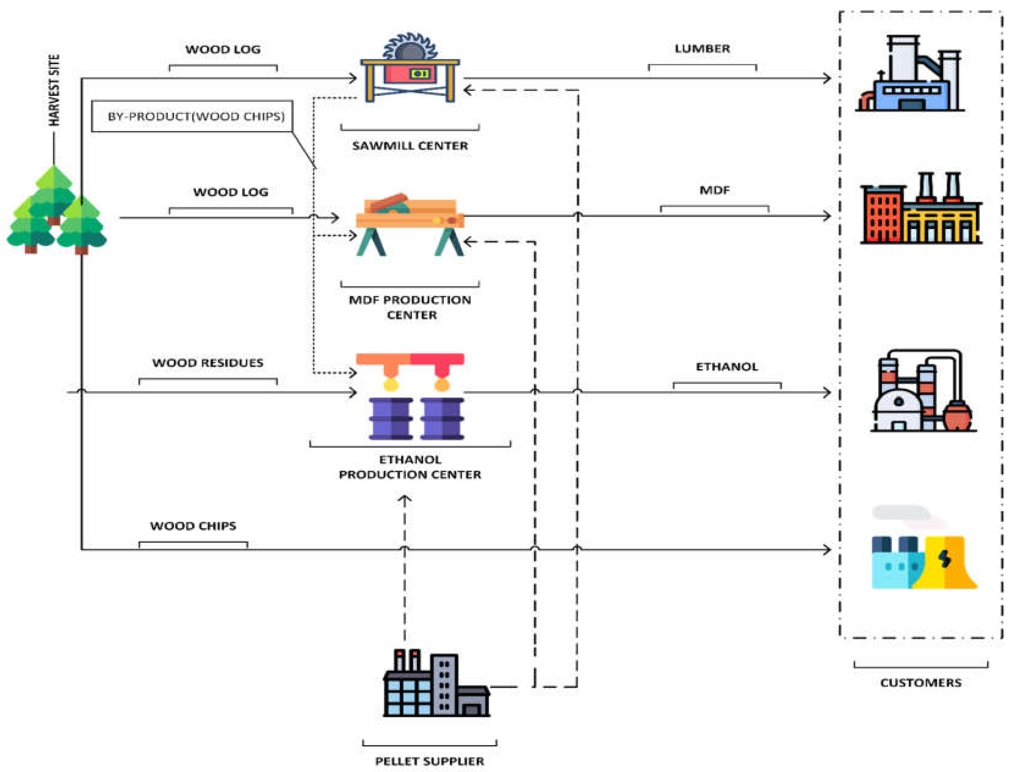
• Designing a sustainable forest supply chain considering log, MDF, and ethanol production facilities;
• Presenting a multi-period multi-product MINLP model, including four objective functions to minimize the profit, improve social aspects, reduce environmental pollution, and minimize lost demands;
• Considering discount in vehicle leasing costs;
• Selecting pellet suppliers based on two elements, order quantity discount and improving social dimensions;
• Considering uncertainty for important parameters that cannot be assumed certain due to their nature.

3. Materials and Methods

A supply chain network was designed based on a multi-period and multi-product Mixed-Integer Non-Linear Programming (MINLP) model for the forest industry, in which the objectives were to maximize profit, minimize detrimental environmental effects, improve social effects, and minimize the number of lost demands so that the chain has all sustainability features. These four objective functions can implement various aspects of forest supply chain sustainability well. Initially, for solving the problem, the multi-objective model was transformed into a single-objective mathematical model by the Epsilon constraint method. Then, for a better and more effective solution, the Lagrange relaxation method was used to reduce the complexity of the problem by relaxing the complex constraints of the problem.

Figure 1 represents the supply chain network that includes harvesting sites, sawmill, MDF production facilities, ethanol production centers, pellet suppliers, customers, and power stations. After determining the appropriate harvesting site, harvesters and wood chippers were assigned to selected sites. Logs harvested by harvesters were sent to the sawmill and MDF production facilities according to demand quantity. As logs were harvested, residues were collected to be sent to ethanol production facilities. Finally, wood wastes were also collected and converted into wood chips by wood chippers. Wood chips were used as the raw materials for power stations. A part of the logs harvested was sent to the sawmill to be converted into lumbers for customers. The by-product of this process was pellets, which can be used as energy sources for MDF and ethanol production facilities. The remaining logs were converted into MDF for sale. Pellets required for supplying the fuel shortage for these facilities were bought from pellet suppliers. The purchasing price of pellets from suppliers was variable depending on order quantity. Suppliers offered different discounts based on order quantity according to their policies. Wood residues were also converted into ethanol via a specific process to be delivered to customers. As stated before, decision making and planning have a particular importance in this industry. Therefore, some decisions were adopted at various levels in each period. One of these decisions was to lease harvesting sites with different capacities and leasing costs from the government. In addition, the number of harvester machines and wood chippers allocated to each harvesting site, the normal working time of machinery and their maximum working hours, and harvest amount should be decided. If required, some machinery to a limited number can be leased to achieve maximum harvesting and profitability. In each period, some trucks used in the supply chain were leased, and their costs varied depending on the quantity discount from suppliers. In the sawmill facility, a portable sawmill can be leased and added to the production line. Furthermore, in the ethanol production facility, the production capacity can be increased to a limited extent by increasing the number of machines. Due to the importance of inventory and storage control of raw materials in each facility, the inventory level of each facility was estimated in each period. Additionally, each facility can increase its inventory to a limited extent by paying the associated cost.

3.1. Mathematical Model

In this section, the proposed MINLP for the forest supply chain is presented. Before exhibiting the objective functions and constraints, indexes, parameters, and decision variables are introduced in

Table 1. Indices of mathematical model.

Indices	Description
I	Set for harvest site
J	Set for sawmill facility
K	Set for MDF production facility
M	Set for ethanol production facility
N	Set for power station
F	Set for harvester machine
R	Set for chipper machine
P	Set for MDF demand zone
D	Set for lumber demand zone
B	Set for ethanol demand zone
A	Set for pellet supplier
C	Set for supplier discount level
Q	Set for renting truck discount level
T	Set for period time

,

Table 2. Parameters of mathematical model.

Parameter	Description
${\mathrm{WT}}_{\mathrm{f}}^{\mathrm{m}}$	Minimum working hours of harvester machine F
${\mathrm{WT}}_{\mathrm{f}}$	Normal working hours of harvester machine F
${\mathrm{WT}}_{\mathrm{f}}^{*}$	Maximum working hours of harvester machine F
${\mathrm{CT}}_{\mathrm{i}}$	Maximum available logs in the harvest site i (${\mathrm{m}}^2$)
$\mathrm{CM}$	Available number of harvester machine F
$\mathrm{RF}$	Coefficient of wood residues obtained per unit of harvested log (m2)
$\mathrm{RN}$	Log harvesting coefficient per hour of harvester machine operation
$\mathrm{RW}$	Coefficient of wood waste obtained from each unit of harvested log that can be converted into wood chips
${\mathrm{KT}}_{\mathrm{r}}$	Normal working hours of chipper machine r
${\mathrm{KT}}_{\mathrm{r}}^{*}$	Maximum working hours of chipper machine r
${\mathrm{KT}}_{\mathrm{r}}^{\mathrm{m}}$	Minimum working hours of chipper machine r
$\mathrm{PCF}$	Conversion rate of wood waste into wood chips per hour of operation of the chipper machine r
$\mathrm{CC}$	Available number of chipper machine r
${\mathrm{SM}}_{\mathrm{j}}$	Number of gangsaw machines located in production line of sawmill J
$\mathrm{PC}$	Conversion rate of log into lumber by gangsaw machine
$\mathrm{PD}$	Conversion rate of log into lumber by portable bandsaw machine
${\mathrm{NZ}}_{\mathrm{j}}$	Number of rentable portable bandsaw machines for sawmill J
$\mathrm{RC}$	Coefficient of lumber obtained per unit of log
$\mathrm{NP}$	The amount of wood chips produced per unit of lumber produced in facility J (kg)
${\mathrm{Ca}}_{\mathrm{j}}$	Maximum storage capacity of logs in sawmill j
$\mathrm{JC}$	Conversion rate of log into MDF by MDF production facilities
$\mathrm{NC}$	Coefficient of MDF obtained per unit of log in facility k
${\mathrm{DK}}_{\mathrm{k}}$	Number of production lines in facility k
${\mathrm{CKK}}_k^{}$	Maximum logs storage capacity in facility k
$\mathrm{DZZ}$	Conversion rate of wood residues into ethanol
${\mathrm{JR}}_{\mathrm{mt}}$	Production capacity of ethanol in facility m in period t
${\mathrm{CT}}_{\mathrm{m}}$	Maximum wood residues inventory capacity in facility m
$\mathrm{EN}$	Energy required to produce each unit MDF
$\mathrm{PK}$	Conversion rate of wood chips into energy
$\mathrm{PN}$	Conversion rate of pellets into energy
$\mathrm{EE}$	Energy required to produce each unit ethanol(L)
${\mathrm{DL}}_{\mathrm{pt}}$	MDF demand in customer zone p in period time t
${\mathrm{DS}}_{dt}$	Lumber demand in customer zone d in period time t
${\mathrm{DKK}}_{\mathrm{bt}}$	Ethanol demand in customer zone b in period time t
${\mathrm{DZ}}_{\mathrm{nt}}$	Wood chips demand by power station n in period time t
$\mathrm{COL}$	Sale price per lumber unit (m2)
$\mathrm{COM}$	Sale price per MDF unit (m2)
$\mathrm{COE}$	Sale price per ethanol unit (L)
$\mathrm{COC}$	Sale price per wood chips unit
$\mathrm{EqO}$	Cost of extra-hours working of the harvester machine
$\mathrm{EqN}$	Cost of regular-hours working of the harvester machine
$\mathrm{ERC}$	Cost of renting harvester machine
$\mathrm{ERH}$	Cost of renting chipper machine
$\mathrm{EqS}$	Cost of extra-hours working of the chipper machine
$\mathrm{EqJ}$	Cost of regular-hours working of the chipper machine
$\mathrm{ERZ}$i	Cost of renting harvest site i
$\mathrm{HCJ}$	Holding cost of logs in sawmill
$\mathrm{HCK}$	Holding cost of logs in facility k
$\mathrm{HCM}$	Holding cost of logs in facility m
$\mathrm{PCN}$	Production cost of each unit lumber(m2)
$\mathrm{PCP}$	Production cost of each unit MDF(m2)
$\mathrm{PCM}$	Production cost of each unit ethanol (L)
$\mathrm{ERK}$	Cost of renting portable bandsaw
$\mathrm{ERS}$	Cost of increasing each unit of storage capacity facility J in each period
$\mathrm{MEC}$i	Maximum possible increase in storage capacity of facility J
$\mathrm{ERP}$	Cost of increasing production capacity in facility m
${\mathrm{PrC}}_{ac}$	Purchase price of each pellet unit as fuel from supplier a, with discount level c
${\mathrm{DSC}}_{af\prime }$	Pellet transportation cost between supplier a and facility $f\prime$
$\mathrm{COP}$	Penalty coefficient for lost demand in zone p
$\mathrm{COD}$	Penalty coefficient for lost demand in zone d
$\mathrm{COB}$	Penalty coefficient for lost demand in zone b
$\mathrm{CON}$	Penalty coefficient for lost demand in power station
${\mathrm{TPC}}_{f,f\prime }$	Transportation cost between facility $f$ and $f\prime$
$\mathrm{KHR}$	Cost of renting log transport truck
$\mathrm{KHN}$	Cost of renting wood residues transport truck
$\mathrm{CF}$	Capacity of lumber transport truck
$\mathrm{CB}$	Capacity of MDF transport truck
$\mathrm{CP}$	Capacity of ethanol transport truck
$\mathrm{CZ}$	Capacity of wood chips transport truck
$\mathrm{CQP}$	Amount of CO2 emission per hour of harvester machine operation
$\mathrm{CQN}$	Amount of CO2 emission per hour of chipper machine operation
$\mathrm{CQZ}$	Amount of CO2 emission per produced lumber unit
$\mathrm{CQM}$	Amount of CO2 emission per produced MDF unit
$\mathrm{CQF}$	Amount of CO2 emission per produced ethanol unit
${\mathrm{CTP}}_{ff\prime }$	Amount of CO2 emission by transportation between $fand f\prime$
$\mathrm{LBR}$	Coefficient of job opportunity per hour harvester machine operation
${\mathrm{BR}}_i$	Unemployment rate in the area where harvester site i is located
$\mathrm{LBC}$	Coefficient of job opportunity per hour chipper machine operation
${\mathrm{REV}}_a$	Regional economic value in supplier a location
${\mathrm{REV}}_{\mathrm{i}}^{\prime }$	Regional economic value in the location of harvest site i
${\mathrm{DRA}}_a$	Development coefficient of the area where the supplier a is located
$\mathrm{AVR}$	Available number of log transport trucks
$\mathrm{CV}$	Capacity of log transport truck
$\mathrm{CN}$	Capacity of wood residues transport truck
$\mathrm{AVL}$	Available number of wood residues transport trucks
${\mathrm{CSK}}_a$	Maximum capacity of supplier a
MECj	Maximum expandable storage capacity sawmill J
${\mathrm{S}}_{act}$	The lower limit of the discount level c for the purchase of pellets, which is set by supplier a in period t
$EZ$	Amount of energy required to reduce log moisture per unit of lumber produced
${\mathrm{UNM}}_q$	Upper bound of rentable lumber transport trucks between facility j and customer zone d with discount interval q
${\mathrm{UNP}}_q$	Upper bound of rentable wood chips transport trucks between harvest site i and power station n with discount interval q
${\mathrm{UNB}}_q$	Upper bound of rentable MDF transport trucks between facility m and customer zone b with discount interval q
${\mathrm{UNN}}_q$	Upper bound of rentable ethanol transport trucks between facility k and customer zone p with discount interval q
${\mathrm{TPCA}}_q$	Rent cost of MDF transport trucks between facility m and customer zone b with discount interval q
${\mathrm{TPCB}}_q$	Rent cost of lumber transport trucks between facility j and customer zone d with discount interval q
${\mathrm{TPCC}}_q$	Rent cost of ethanol transport trucks between facility k and customer zone p with discount interval q
${\mathrm{TPCD}}_q$	Rent cost of wood chips transport trucks between harvest site i and customer zone n with discount interval q

and

Table 3. Variables of mathematical model.

Variable	Description
${\mathrm{FT}}_{\mathrm{fit}}$	Total hours used by harvester machine F in harvest site i in period t
${\mathrm{FT}}_{\mathrm{fit}}^{*}$	Extra hours used by harvester machine F in harvest site i in period t
${\mathrm{RM}}_{\mathrm{t}}$	Number of rented harvester machines in period t
${\mathrm{CK}}_{\mathrm{rit}}$	Total hours used by chipper machine r in harvest site i in period t
${\mathrm{Ck}}_{\mathrm{rit}}^{*}$	Extra hours used by chipper machine r in harvest site i in period t
${\mathrm{ZM}}_{\mathrm{t}}$	Number of rented chipper machines in period t
${\mathrm{IJ}}_{\mathrm{jt}}$	Log inventory in facility j in period t (m2)
${\mathrm{FZ}}_{\mathrm{jt}}$	Number of rented portable bandsaws for facility j in period t
${\mathrm{FA}}_{\mathrm{it}}$	Number of harvested logs in harvest site i (m2)
${\mathrm{FB}}_{\mathrm{ijt}}$	Number of logs transported from harvest site i to sawmill j in period t
${\mathrm{FC}}_{\mathrm{ikt}}$	Number of logs transported from harvest site i to MDF production facility k in period t
${\mathrm{FE}}_{\mathrm{imt}}$	Amount of wood residues transported from harvest site i to facility m in period t
${\mathrm{FF}}_{\mathrm{it}}$	Amount of wood waste in harvest site i can be converted into wood chips in period t
${\mathrm{FH}}_{\mathrm{jdt}}$	Amount of lumber transported from sawmill j to demand zone d in period t
${\mathrm{FM}}_{\mathrm{jkt}}$	Amount of by-product (wood chips) transported from sawmill j to facility k in period t
${\mathrm{FP}}_{\mathrm{jmt}}$	Amount of by-product (wood chips) transported from sawmill j to facility m in period t
${\mathrm{IK}}_{\mathrm{kt}}$	Log inventory in facility k in period t
${\mathrm{Fq}}_{\mathrm{kpt}}$	Amount of MDF transported from facility k to demand zone p in period t
${\mathrm{IM}}_{\mathrm{mt}}$	Wood residues inventory in facility m in period t
${\mathrm{FS}}_{\mathrm{mbt}}$	Amount of produced ethanol transported from facility m to demand zone b in period time t
${\mathrm{EJ}}_{\mathrm{mt}}$	Increase production capacity in facility m in period time t
${\mathrm{FD}}_{\mathrm{akt}}$	Amount of pellets purchased from supplier a to supply energy in facility k in period t (Kg)
${\mathrm{FR}}_{\mathrm{amt}}$	Amount of pellets purchased from supplier a to supply energy in facility m in period t (Kg)
$\mathrm{F}{V}_{\mathrm{ajt}}$	Amount of pellets purchased from supplier a to supply energy in facility j in period t (Kg)
${\mathrm{LA}}_{\mathrm{pt}}$	Lost demand in customer zone p in period t
${\mathrm{LB}}_{\mathrm{dt}}$	Lost demand in customer zone d in period t
${\mathrm{LC}}_{\mathrm{bt}}$	Lost demand in customer zone b in period t
${\mathrm{LD}}_{\mathrm{nt}}$	Lost demand in power station n in period t
$V{R}_{\mathrm{ijt}}$	Number of log transport trucks assigned to transportation route between harvest site i and sawmill j
$V{K}_{\mathrm{ikt}}$	Number of log transport trucks assigned to transportation route between harvest site i and MDF production center k
$V{F}_{\mathrm{imt}}$	Number of wood residues transport trucks assigned to transportation route between harvest site i and sawmill j
$RV{R}_{\mathrm{t}}$	Number of rented log transport trucks in period time t
${\mathrm{RVL}}_{\mathrm{t}}$	Number of rented wood residues transport trucks in period time t
${\mathrm{VA}}_{\mathrm{jdt}}$	Number of rented lumber transport trucks from facility j to customer zone d in period time t
${\mathrm{VE}}_{\mathrm{kpt}}$	Number of rented MDF transport trucks from facility k to customer zone p in period time t
${\mathrm{VV}}_{\mathrm{mbt}}$	Number of rented ethanol transport trucks from facility m to customer zone b in period time t
${\mathrm{VZ}}_{\mathrm{jnt}}$	Number of rented wood chips transport trucks from harvest site i to power station n in period time t
${\mathrm{VI}}_{\mathrm{jkt}}$	Number of rented wood chips transport trucks from facility j to facility k in period time t
${\mathrm{VO}}_{\mathrm{jmt}}$	Number of rented wood chips transport trucks from facility j to facility m in period time t
${\mathrm{FG}}_{\mathrm{int}}$	Amount of wood chips transported from harvest site i to power station n in period t
${\mathrm{EC}}_{\mathrm{jt}}$	Increased inventory capacity in facility j in period time t
${\mathrm{Z}}_{\mathrm{fit}}$	If the harvester machine F is assigned to harvest site i in period t, 1; otherwise, 0
$\mathrm{G}$i	If harvest site i is rented in period t, 1; otherwise, 0
$y_{\mathrm{rit}}$	If chipper machine r is assigned to harvest site i in period t, 1; otherwise, 0
${\mathrm{H}}_{\mathrm{at}}$	If supplier a is selected in period t, 1; otherwise, 0
${\mathrm{QR}}_{\mathrm{act}}$	If discount level c is considered for purchase from supplier a in period t,1; otherwise, 0
${\mathrm{HLM}}_{\mathrm{qt}}$	1, if required trucks between facility j and demand zone d are rented at discount level q in period t; otherwise, 0
${\mathrm{HLN}}_{\mathrm{qt}}$	1, if required trucks between facility k and demand zone p are rented at discount level q in period t; otherwise, 0
${\mathrm{HLB}}_{\mathrm{qt}}$	1, if required trucks between facility m and demand zone b are rented at discount level q in period t; otherwise, 0
${\mathrm{HLP}}_{\mathrm{qt}}$	1, if required trucks between harvest site i and power station n are rented at discount level q in period t; otherwise, 0

.

The suggested MINLP model includes four objective functions, i.e., maximizing the profit, minimizing pollutant gas emissions, improving social dimensions, and minimizing lost demands. Equation (1) calculates the net profit earned by selling each product, including each unit of logs, MDF, ethanol, and wood chips, based on their purchasing price.

$$PFS={\displaystyle {\displaystyle \sum }_j}{\displaystyle {\displaystyle \sum }_d}{\displaystyle {\displaystyle \sum }_t}F{H}_{jdt}\times COL+{\displaystyle {\displaystyle \sum }_k}{\displaystyle {\displaystyle \sum }_{\rho }}{\displaystyle {\displaystyle \sum }_t}F{q}_{k\rho t}\times COM+{\displaystyle {\displaystyle \sum }_m}{\displaystyle {\displaystyle \sum }_b}{\displaystyle {\displaystyle \sum }_t}F{S}_{mbt}\times COE+{\displaystyle {\displaystyle \sum }_i}{\displaystyle {\displaystyle \sum }_n}{\displaystyle {\displaystyle \sum }_t}F{G}_{int}\times COC$$

(1)

Equation (2) measures the utilization costs of harvester and wood chipper machinery per usual working time and overtime. The cost of leasing the machinery and harvesting sites is also included in this equation.

$$\begin{gathered} CHS={\displaystyle {\displaystyle \sum }_f}{\displaystyle {\displaystyle \sum }_i}{\displaystyle {\displaystyle \sum }_t}F{T}_{fit}\times EqN+{\displaystyle {\displaystyle \sum }_f}{\displaystyle {\displaystyle \sum }_i}{\displaystyle {\displaystyle \sum }_t}F{T}_{fit}^{*}\times EqO+{\displaystyle {\displaystyle \sum }_r}{\displaystyle {\displaystyle \sum }_i}{\displaystyle {\displaystyle \sum }_t}C{K}_{rit}\times EqJ+{\displaystyle {\displaystyle \sum }_r}{\displaystyle {\displaystyle \sum }_i}{\displaystyle {\displaystyle \sum }_t}C{K}_{rit}^{*}\times EqS \\ +{\displaystyle {\displaystyle \sum }_t}R{M}_t\times ERC+{\displaystyle {\displaystyle \sum }_t}\Omega M_t\times ERH+{\displaystyle {\displaystyle \sum }_i}{G}_i\times ER{\Omega }_i \end{gathered}$$

(2)

Equation (3) considers the cost of production, inventory, increase in storage and production capacity at each facility.

$$\begin{gathered} CIF={\displaystyle {\displaystyle \sum }_j}{\displaystyle {\displaystyle \sum }_t}{I}_{jt}\times HC+{\displaystyle {\displaystyle \sum }_j}{\displaystyle {\displaystyle \sum }_d}{\displaystyle {\displaystyle \sum }_t}F{H}_{jdt}\times PCM+{\displaystyle {\displaystyle \sum }_j}{\displaystyle {\displaystyle \sum }_t}F{\Omega }_{jt}\times ERK+{\displaystyle {\displaystyle \sum }_j}{\displaystyle {\displaystyle \sum }_t}E{C}_{jt}\times ERS+{\displaystyle {\displaystyle \sum }_k}{\displaystyle {\displaystyle \sum }_t}{I}_{kt} \\ \times HCK+{\displaystyle {\displaystyle \sum }_k}{\displaystyle {\displaystyle \sum }_{\rho }}{\displaystyle {\displaystyle \sum }_t}F{q}_{k\rho t}\times \rho c\rho +{\displaystyle {\displaystyle \sum }_m}{\displaystyle {\displaystyle \sum }_t}I{M}_{mt}\times HCM+{\displaystyle {\displaystyle \sum }_m}{\displaystyle {\displaystyle \sum }_b}{\displaystyle {\displaystyle \sum }_t}F{S}_{mbt}\times \rho cN \\ +{\displaystyle {\displaystyle \sum }_m}{\displaystyle {\displaystyle \sum }_t}E{J}_{mt}\times ERP \end{gathered}$$

(3)

Equation (4) calculates the cost of ordering pellets from external supplier according to the quantity discount level.

$$SEFF={\displaystyle {\displaystyle \sum }_a}{\displaystyle {\displaystyle \sum }_c}{\displaystyle {\displaystyle \sum }_t}Pr{c}_{ac}\times Q{R}_{act}\times \left[{\displaystyle {\displaystyle \sum }_k}F{D}_{akt}+{\displaystyle {\displaystyle \sum }_m}F{R}_{amt}+{\displaystyle {\displaystyle \sum }_j}F{V}_{ajt}\right]$$

(4)

Equation (5) also represents the cost of transport between facilities. The transportation cost between harvesting sites, sawmills, MDF facilities, and ethanol facilities was considered in terms of the number of trucks. The quantity discount for the leased trucks, which was determined by the supplier according to the number of trucks, is considered in Equation (5).

$$\begin{gathered} TPCS={\displaystyle {\displaystyle \sum }_j}{\displaystyle {\displaystyle \sum }_j}{\displaystyle {\displaystyle \sum }_t}V{R}_{ijt}\times TP{C}_{ij}+{\displaystyle {\displaystyle \sum }_i}{\displaystyle {\displaystyle \sum }_k}{\displaystyle {\displaystyle \sum }_t}V{K}_{ikt}\times TP{C}_{ik}+{\displaystyle {\displaystyle \sum }_t}RV{R}_t\times KHR+{\displaystyle {\displaystyle \sum }_t}RV{L}_t\times KHN \\ +{\displaystyle {\displaystyle \sum }_i}{\displaystyle {\displaystyle \sum }_m}{\displaystyle {\displaystyle \sum }_t}V{F}_{imt}\times TP{C}_{im}+ \\ {\displaystyle {\displaystyle \sum }_m}{\displaystyle {\displaystyle \sum }_b}{\displaystyle {\displaystyle \sum }_t}{\displaystyle {\displaystyle \sum }_q}V{V}_{mbt}\times HL{B}_{qt}\times TPCA+{\displaystyle {\displaystyle \sum }_j}{\displaystyle {\displaystyle \sum }_d}{\displaystyle {\displaystyle \sum }_t}{\displaystyle {\displaystyle \sum }_q}V{A}_{jdt}\times HL{M}_{qt}\times TPC{B}_q \\ +{\displaystyle {\displaystyle \sum }_k}{\displaystyle {\displaystyle \sum }_{\rho }}{\displaystyle {\displaystyle \sum }_q}{\displaystyle {\displaystyle \sum }_t}V{E}_{k\rho t}\times HL{N}_{qt}\times TPC{C}_q+{\displaystyle {\displaystyle \sum }_i}{\displaystyle {\displaystyle \sum }_n}{\displaystyle {\displaystyle \sum }_t}{\displaystyle {\displaystyle \sum }_q}V{\Omega }_{int}\times HL{\rho }_{qt}\times TPCD+ \\ {\displaystyle {\displaystyle \sum }_i}{\displaystyle {\displaystyle \sum }_k}{\displaystyle {\displaystyle \sum }_t}V{I}_{jkt}\times T\rho C_{jk}+{\displaystyle {\displaystyle \sum }_j}{\displaystyle {\displaystyle \sum }_m}{\displaystyle {\displaystyle \sum }_t}V{O}_{jmt}\times T\rho C_{jm} \end{gathered}$$

(5)

Therefore, the first objective function that tries to maximize the profit of the forest supply chain is formulated as Equation (6).

$$\mathrm{Max}{Z}_1=\mathrm{PFS}-\mathrm{CHS}-\mathrm{CIF}-\mathrm{SEFF}-\mathrm{TPCS}$$

(6)

The second objective function aimed to minimize environmental impacts in the whole of the network by minimizing the CO₂ emitted by machinery per working hour, per unit of products, and pollution caused by transportation. This objective function is formulated as below (Equation (7)):

$$\begin{gathered} Min Z_2={\displaystyle {\displaystyle \sum }_f}{\displaystyle {\displaystyle \sum }_i}{\displaystyle {\displaystyle \sum }_t}\left(F{T}_{fit}+F{T}_{fit}^{*}\right)\times CQ\rho +{\displaystyle {\displaystyle \sum }_r}{\displaystyle {\displaystyle \sum }_i}{\displaystyle {\displaystyle \sum }_t}\left(C{K}_{rit}+C{K}_{rit}^{*}\right)\times CQN \\ +{\displaystyle {\displaystyle \sum }_j}{\displaystyle {\displaystyle \sum }_d}{\displaystyle {\displaystyle \sum }_t}F{H}_{jdt}\times CQ\Omega +{\displaystyle {\displaystyle \sum }_k}{\displaystyle {\displaystyle \sum }_{\rho }}{\displaystyle {\displaystyle \sum }_t}F{q}_{k\rho t}\times CQM+{\displaystyle {\displaystyle \sum }_m}{\displaystyle {\displaystyle \sum }_b}{\displaystyle {\displaystyle \sum }_t}F{S}_{mbt}\times CQF \\ +{\displaystyle {\displaystyle \sum }_i}{\displaystyle {\displaystyle \sum }_j}{\displaystyle {\displaystyle \sum }_t}V{R}_{ijt}\times CT{P}_{ij}+{\displaystyle {\displaystyle \sum }_i}{\displaystyle {\displaystyle \sum }_k}{\displaystyle {\displaystyle \sum }_t}V{K}_{ikt}\times CT{P}_{ik}+{\displaystyle {\displaystyle \sum }_i}{\displaystyle {\displaystyle \sum }_m}{\displaystyle {\displaystyle \sum }_t}V{F}_{imt}\times CT{P}_{im} \\ +{\displaystyle {\displaystyle \sum }_j}{\displaystyle {\displaystyle \sum }_d}{\displaystyle {\displaystyle \sum }_t}V{A}_{jdt}\times CT{P}_{jdt}+{\displaystyle {\displaystyle \sum }_k}{\displaystyle {\displaystyle \sum }_{\rho }}{\displaystyle {\displaystyle \sum }_t}V{E}_{k\rho t}\times CT{P}_{k\rho t}+{\displaystyle {\displaystyle \sum }_m}{\displaystyle {\displaystyle \sum }_b}{\displaystyle {\displaystyle \sum }_t}V{V}_{mbt}\times CT{P}_{mb} \\ +{\displaystyle {\displaystyle \sum }_i}{\displaystyle {\displaystyle \sum }_n}{\displaystyle {\displaystyle \sum }_t}V{\Omega }_{int}\times CT{P}_{in}+{\displaystyle {\displaystyle \sum }_j}{\displaystyle {\displaystyle \sum }_k}{\displaystyle {\displaystyle \sum }_t}V{I}_{jkt}\times CT{P}_{jk}+{\displaystyle {\displaystyle \sum }_j}{\displaystyle {\displaystyle \sum }_m}{\displaystyle {\displaystyle \sum }_t}V{O}_{jmt}\times CT{P}_{jm} \end{gathered}$$

(7)

The third objective function was associated with social effects involving two aspects. The first aspect (Equation (8)) was related to the unemployment rate and job opportunities created by the activities of machinery in harvest sites.

$$NF={\displaystyle {\displaystyle \sum }_f}{\displaystyle {\displaystyle \sum }_i}{\displaystyle {\displaystyle \sum }_t}F{T}_{fit}\times LBR\times B{R}_i+{\displaystyle {\displaystyle \sum }_r}{\displaystyle {\displaystyle \sum }_i}{\displaystyle {\displaystyle \sum }_t}C{K}_{rit}\times LBC\times B{R}_i$$

(8)

The second aspect (Equation (9)) also depended on the regional economic development indicator for the regions where the harvesting site and pellet suppliers were located. In other words, leasing the harvesting sites or selecting the suppliers located in less-developed regions improved the social impacts.

$$\begin{gathered} K\Omega F={\displaystyle {\displaystyle \sum }_a}{\displaystyle {\displaystyle \sum }_t}RE{V}_a\times \left(1-DR{A}_a\right)H_{at}+{\displaystyle {\displaystyle \sum }_f}{\displaystyle {\displaystyle \sum }_i}{\displaystyle {\displaystyle \sum }_t}{\Omega }_{fit}\times RE{V}_i^{\prime }\left(1-DR{A}_i^{\prime }\right) \\ +{\displaystyle {\displaystyle \sum }_r}{\displaystyle {\displaystyle \sum }_i}{\displaystyle {\displaystyle \sum }_t}{y}_{rit}\times RE{V}_i^{\prime }\times \left(1-DR{A}_i^{\prime }\right) \end{gathered}$$

(9)

Finally, the third objective function is formulated as follows (Equation (10)):

$$Min Z_3=\frac{{\left[KNF\right]}^{max}-\left[KNF\right]}{{\left[KNF\right]}^{max}-{\left[KNF\right]}^{min}}+\frac{{\left[K\Omega F\right]}^{max}-\left[K\Omega F\right]}{{\left[K\Omega F\right]}^{max}-{\left[K\Omega F\right]}^{min}}$$

(10)

As seen in Equation (10), the objective function related to social effects is constructed as $\left(Z^{max}-Z\right)/\left(Z^{max}-Z^{min}\right)$. The minimum value of this fraction was associated with the maximum value of $Z$. First, the value of $Z^{min}$ and $Z^{max}$ were obtained separately. Then, their values were replaced in the equation as constant values. Next, the maximum value of $Z$ was obtained by minimizing the objective function. The fourth objective function also attempted to minimize customers’ unmet demands. This objective function is written as follows (Equation (11)):

$$\begin{gathered} Min Z_4={\displaystyle {\displaystyle \sum }_{\rho }}{\displaystyle {\displaystyle \sum }_t}L{A}_{\rho t}\times COP+{\displaystyle {\displaystyle \sum }_d}{\displaystyle {\displaystyle \sum }_t}L{R}_{dt}\times COD \\ +{\displaystyle {\displaystyle \sum }_b}{\displaystyle {\displaystyle \sum }_t}L{C}_{bt}\times COB+{\displaystyle {\displaystyle \sum }_n}{\displaystyle {\displaystyle \sum }_t}L{D}_{nt}\times CON \end{gathered}$$

(11)

Following the description of the mathematical model, the equations are presented in

Table 4. Constraints of mathematical model.

Equation (12)	${\Omega }_{fit}.w{T}_f^m\le F{T}_{fit}\le \left(w{T}_f+w{T}_f^{*}\right){\Omega }_{fit}$	$\forall f,i,t$
Equation (13)	$F{T}_{fit}-w{T}_f\le F{T}_{fit}^{*}\le W{T}_f^{*}$	$\forall f,i,t$
Equation (14)	$F{A}_{it}={\displaystyle {\displaystyle \sum }_f}F{T}_{fit}\times Rn$	$\forall i,t$
Equation (15)	$F{A}_{it}={\displaystyle {\displaystyle \sum }_j}F{B}_{ijt}+{\displaystyle {\displaystyle \sum }_k}F{C}_{ikt}$	$\forall i,t$
Equation (16)	$F{A}_{it}\times RF\ge {\displaystyle {\displaystyle \sum }_m}F{E}_{imt}$	$\forall i,t$
Equation (17)	$F{A}_{it}.RW=F{F}_{it}$	$\forall i,t$
Equation (18)	${\displaystyle {\displaystyle \sum }_t}F{A}_{it}\le C{T}_i\times G_i$	$\forall i$
Equation (19)	${\displaystyle {\displaystyle \sum }_i}{\displaystyle {\displaystyle \sum }_f}{\Omega }_{fit}\le CM+R{M}_t$	$\forall t$
Equation (20)	${\displaystyle {\displaystyle \sum }_i}{\Omega }_{fit}\le 1$	$\forall f,t$
Equation (21)	$y_{rit}\times k{T}_r^m\le C{K}_{rit}\le \left(K{T}_r+K{T}_r^{*}\right)y_{rit}$	$\forall r,i,t$
Equation (22)	$C{K}_{rit}-K{T}_r\le C{K}_{rit}^{*}\le K{T}_r^{*}$	$\forall r,i,t$
Equation (23)	${\displaystyle {\displaystyle \sum }_n}F{G}_{int}\le {\displaystyle {\displaystyle \sum }_r}C{K}_{rit}\times PCF$	$\forall i,t$
Equation (24)	${\displaystyle {\displaystyle \sum }_r}C{K}_{rit}\times PCF\le F{F}_{it}$	$\forall i,t$
Equation (25)	${\displaystyle {\displaystyle \sum }_r}{\displaystyle {\displaystyle \sum }_i}{y}_{rit}\le CC+\Omega M_t$	$\forall t$
Equation (26)	${\displaystyle {\displaystyle \sum }_i}{y}_{rit}\le 1$	$\forall r,t$
Equation (27)	$I{J}_{Jt}=I{J}_{J\left(t-1\right)}+{\displaystyle {\displaystyle \sum }_i}F{B}_{ijt}-\frac{{{\displaystyle \sum }}_{d}F{H}_{jdt}}{RC}$	$\forall j,t$
Equation (28)	$I{J}_{jt}\le c{a}_j+E{c}_{jt}$	$\forall j,t$
Equation (29)	$E{C}_{jt}\le ME{C}_j$	$\forall j,t$
Equation (30)	${\displaystyle {\displaystyle \sum }_d}F{H}_{jdt}\le PC\times S{M}_j+PP\times F{\Omega }_{jt}$	$\forall j,t$
Equation (31)	$F{\Omega }_{jt}\le N{\Omega }_j$	$\forall j,t$
Equation (32)	${\displaystyle {\displaystyle \sum }_d}F{H}_{jdt}\times N\rho \ge {\displaystyle {\displaystyle \sum }_k}F{M}_{jkt}+{\displaystyle {\displaystyle \sum }_m}F{\rho }_{jmt}$	$\forall j,t$
Equation (33)	$I{K}_{kt}=I{K}_{k\left(t-1\right)}+{\displaystyle {\displaystyle \sum }_i}F{C}_{ikt}-\frac{{{\displaystyle \sum }}_{\rho }F{Q}_{k\rho t}}{JC}$	$\forall k,t$
Equation (34)	$F{q}_{k\rho t}\le D{K}_k.NC$	$\forall k,p,t$
Equation (35)	$I{K}_{kt}\le CK{K}_k$	$\forall k,t$
Equation (36)	$I{M}_{mt}=I{M}_{m\left(t-1\right)}+{\displaystyle {\displaystyle \sum }_i}F{E}_{imt}-\frac{{{\displaystyle \sum }}_{b}F{S}_{mbt}}{D\Omega \Omega }$	$\forall m,t$
Equation (37)	$I{M}_{mt}\le C{J}_m$	$\forall m,t$
Equation (38)	${\displaystyle {\displaystyle \sum }_b}F{S}_{mbt}\le J{R}_m+E{J}_{mt}$	$\forall m,t$
Equation (39)	${\displaystyle {\displaystyle \sum }_{\rho }}F{q}_{k\rho t}\times EN={\displaystyle {\displaystyle \sum }_j}F{M}_{jkt}\times Pk+{\displaystyle {\displaystyle \sum }_a}F{D}_{akt}\times PN$	$\forall k,t$
Equation (40)	${\displaystyle {\displaystyle \sum }_b}F{S}_{mbt}\times EE={\displaystyle {\displaystyle \sum }_j}F{\rho }_{jmt}\times Pk+{\displaystyle {\displaystyle \sum }_a}F{R}_{am}\times PN$	$\forall m,t$
Equation (41)	${\displaystyle {\displaystyle \sum }_d}F{H}_{jdt}\times E\Omega ={\displaystyle {\displaystyle \sum }_a}F{V}_{ajt}\times PN$	$\forall j,t$
Equation (42)	${\displaystyle {\displaystyle \sum }_k}F{q}_{k\rho t}+L{A}_{\rho t}=D{L}_{\rho t}$	$\forall p,t$
Equation (43)	${\displaystyle {\displaystyle \sum }_j}F{H}_{jdt}+L{B}_{dt}=D{S}_{dt}$	$\forall d,t$
Equation (44)	${\displaystyle {\displaystyle \sum }_m}F{S}_{mbt}+L{C}_{bt}=DK{K}_{bt}$	$\forall b,t$
Equation (45)	${\displaystyle {\displaystyle \sum }_i}F{G}_{int}+L{D}_{nt}=D{Z}_{nt}$	$\forall n,t$
Equation (46)	$F{B}_{ijt}\le V{R}_{ijt}.CV$	$\forall i,j,t$
Equation (47)	$F{C}_{ikt}\le V{K}_{ikt}.CV$	$\forall i,k,t$
Equation (48)	${\displaystyle {\displaystyle \sum }_i}{\displaystyle {\displaystyle \sum }_k}V{K}_{ikt}+{\displaystyle {\displaystyle \sum }_i}{\displaystyle {\displaystyle \sum }_j}V{R}_{ijt}\le AVR+RV{R}_t$	$\forall t$
Equation (49)	$F{B}_{ijt}\times BigM\ge V{R}_{ijt}$	$\forall i,j,t$
Equation (50)	$F{C}_{ikt}\times BigM\ge V{K}_{ikt}$	$\forall i,k,t$
Equation (51)	$F{E}_{imt}\le V{F}_{imt}.CN$	$\forall i,m,t$
Equation (52)	${\displaystyle {\displaystyle \sum }_i}{\displaystyle {\displaystyle \sum }_m}V{F}_{imt}\le AVL+RV{L}_t$	$\forall t$
Equation (53)	$F{E}_{imt}\times BigM\ge V{F}_{imt}$	$\forall i,m,t$
Equation (54)	${\displaystyle {\displaystyle \sum }_k}F{D}_{akt}+{\displaystyle {\displaystyle \sum }_m}F{R}_{amt}+{\displaystyle {\displaystyle \sum }_j}F{V}_{ajt}\le CS{K}_a\times H_{at}$	$\forall a,t$
Equation (55)	$Q{R}_{act}\times {\delta }_{act}\le F{X}_{at}$	$\forall a,c,t$
Equation (56)	$F{X}_{at}={\displaystyle {\displaystyle \sum }_k}F{D}_{akt}+{\displaystyle {\displaystyle \sum }_m}F{R}_{amt}+{\displaystyle {\displaystyle \sum }_j}F{V}_{ajt}$	$\forall a,t$
Equation (57)	${\displaystyle {\displaystyle \sum }_c}Q{R}_{act}=H_{at}$	$\forall a,t$
Equation (58)	$F{H}_{jdt}\le V{A}_{jdt}\times CF$	$\forall j,d,t$
Equation (59)	$F{q}_{k\rho t}\le V{E}_{k\rho t}\times CB$	$\forall k,\rho ,t$
Equation (60)	$F{S}_{mbt}\le V{V}_{mbt}\times CP$	$\forall m,b,t$
Equation (61)	$F{G}_{int}\le V{\Omega }_{int}\times CZ$	$\forall i,n,t$
Equation (62)	$F{M}_{jkt}\le V{I}_{jkt}\times CZ$	$\forall j,k,t$
Equation (63)	$F{\rho }_{jmt}\le V{o}_{jmt}\times CZ$	$\forall j,m,t$
Equation (64)	$E{J}_{mt}\le AN{N}_m$	$\forall m,t$
Equation (65)	$Gi\le {\displaystyle {\displaystyle \sum }_f}{\displaystyle {\displaystyle \sum }_t}{\Omega }_{fit}\le bigm\times Gi$	$\forall i$
Equation (66)	$UN{M}_{\left(q-1\right)}+bigm\left(HL{M}_{qt}-1\right)\le {\displaystyle {\displaystyle \sum }_j}{\displaystyle {\displaystyle \sum }_d}V{A}_{jdt}$	$\forall q,t$
Equation (67)	${\displaystyle {\displaystyle \sum }_j}{\displaystyle {\displaystyle \sum }_d}V{A}_{jdt}\le UN{M}_q+bigm\left(1-HL{M}_{qt}\right)$	$\forall q,t$
Equation (68)	$UNP+bigm\left(HL{P}_{qt}-1\right)\le {\displaystyle {\displaystyle \sum }_i}{\displaystyle {\displaystyle \sum }_n}V{\xi }_{int}$	$\forall t,q$
Equation (69)	${\displaystyle {\displaystyle \sum }_i}{\displaystyle {\displaystyle \sum }_n}V{\Omega }_{int}\le UN{P}_q+bigm\left(1-HL{P}_{qt}\right)$	$\forall t,q$
Equation (70)	$UN{B}_{\left(q-1\right)}+bigm\left(HL{B}_{qt}-1\right)\le {\displaystyle {\displaystyle \sum }_m}{\displaystyle {\displaystyle \sum }_b}V{V}_{mbt}$	$\forall m,b$
Equation (71)	${\displaystyle {\displaystyle \sum }_m}{\displaystyle {\displaystyle \sum }_b}V{V}_{mbt}\le UN{B}_q+bigm\left(1-HL{B}_{qt}\right)$	$\forall m,b$
Equation (72)	$UN{N}_{\left(q-1\right)}+bigm\left(HL{N}_{qt}-1\right)\le {\displaystyle {\displaystyle \sum }_k}{\displaystyle {\displaystyle \sum }_{\rho }}V{E}_{kpt}$	$\forall q,t$
Equation (73)	${\displaystyle {\displaystyle \sum }_k}{\displaystyle {\displaystyle \sum }_{\rho }}V{E}_{k\rho t}\le UN{N}_q+bigm\left(1-HL{N}_{qt}\right)$	$\forall q,t$
Equation (74)	${\displaystyle {\displaystyle \sum }_q}HL{M}_{qt}=1$	$\forall t$
Equation (75)	${\displaystyle {\displaystyle \sum }_q}HL{P}_{qt}=1$	$\forall t$
Equation (76)	${\displaystyle {\displaystyle \sum }_q}HL{B}_{qt}=1$	$\forall t$
Equation (77)	${\displaystyle {\displaystyle \sum }_q}HL{N}_{qt}=1$	$\forall t$

, which are the constraints of the proposed model.

Equations (12) and (13) were considered to determine the working time and overtime of each harvesting machine if they were allocated to harvesting sites. Equation (14) specified the harvesting quantity of logs in each period. Equation (15) guaranteed that, in each period time, the volume of logs transported to facilities k and j equaled the volume of logs harvested in that period time. Equation (16) ensured that the maximum amount of wood residue that could be transported to ethanol facilities was equal to the volume of produced wood residue. Equation (17) also determined the volume of wood waste convertible into wood chips. Equation (18) states that the maximum harvest volume from each harvest site was equal to the volume of harvestable logs. Equation (19) emphasized that the number of harvest machinery allocated to harvesting sites in each period time did not exceed the number of available and rentable machines. Equations (21) and (22) were, respectively, used to determine the working time for each wood chipper and its overwork if they were allocated to harvesting sites. Equation (23) determined the volume of wood chips transportable from harvesting sites to power stations. Equation (24) made sure that the volume of produced wood chips in each period time did not exceed the volume of wood wastes. Equation (25) ensured that the number of wood chippers allocated in each period did not surpass the number of existing or leased machines. Equation (26) also indicated that each wood chipper could only be allocated to one harvesting site in each period time. Equations (27)–(29) were, respectively considered to determine the inventory level in the sawmill facility, maximum inventory capacity, and maximum allowable increase in inventory capacity. Equation (30) represented the maximum production capacity of facility j. Equation (31) showed the maximum number of leasable portable bandsaws that could be added to facility j. Equation (32) specified the volume of pellets that were generated with each produced lumber and could be sent to facilities k and m as fuel. Equation (33) represented the balance level for inventory at facility k. Equation (34) showed the production and sending level in facility k in each period. Equation (35) indicated the maximum inventory storage capacity for facility k. Equations (36) and (37) represented the inventory level and maximum allowable inventory level in facility m. Equations (39)–(41) specified the volume of energy required for production in facilities m, j, and k. Equations (42)–(45) also determined the demand satisfaction for each product considering the number of lost demands. Equations (46) and (47) set the capacity and number of trucks carrying logs. Equation (48) ensured that the number of trucks carrying logs did not exceed the number of available and leased trucks. Equations (49) and (50) ensured that the trucks were allocated to log routes if there was a product to be transported on that route. Equation (51) was associated with the capacity of trucks carrying wood residues. Equation (53) guaranteed that the trucks carrying wood residues were assigned to a route if there was a product to be transported on that route. Equation (54) indicated the maximum production capacity of pellets by each supplier if selected. Equations (55) and (56) also specified the order quantity for each pellet supplier and its discount range. Equation (57) ensured that only one discount level from each pellet supplier could be chosen. Equations (58)–(61) indicated the capacity of the trucks carrying the orders from each facility to a demand node. Equations (62) and (63) also determined the capacity of the trucks carrying wood chips from facility j to facilities m and k and specified the volume that could be carried. Equation (64) showed the maximum allowable increase in the inventory level of facility m in each period. Equation (65) also made sure that the harvester machines were allocated to harvesting sites if the site was leased. Finally, Equations (66)–(73) set the discount on the number of leased machines between the existing nodes. Equations (73)–(77) ensured that only one discount level could be chosen for renting trucks.

3.2. Hybrid Robust Possibilistic Programming (HRPP-II)

In this research, the demand quantity for each product, the harvesting rate of each harvester machine, and the transformation rate of each wood chipper machine were considered uncertain. These parameters were determined based on historical data or previously accessed data. The value of these parameters could increase or decrease due to some changes. For example, the demand parameters whose value was different for various products could have been overestimated or underestimated due to incorrect estimation, changes in demanders’ behavior, or other changes. Underestimating these parameters relative to the real value could lead to the inability to fulfill demands and consequently cause the lost demands to increase. On the other hand, demand overestimation could increase holding, transportation, and ordering costs unreasonably. Both situations damaged the supply chain and affected predetermined goals. The incorrect estimation of the capacity and performance of machinery at harvesting sites also led to instability and a decrease in supply power. A robust approach was adapted in the mathematical model to deal with data uncertainty. Assume that the following model (Equation (78)) is a mathematical model considering uncertain parameters:

$$\begin{array}{c}Min F=B\times Z\hfill \\ S.t:\hfill \\ A\times Z\ge C\hfill \\ Z\ge 0\hfill \end{array}$$

(78)

Uncertain parameters had a trapezoidal probability distribution as follows (Equation (79)):

$$P_{\xi }\left(x\right)=\{\begin{array}{c}\frac{x-{\xi }_1}{{\xi }_2-{\xi }_1} if {\xi }_1\le x\le {\xi }_2\\ 1 if {\xi }_2\le x\le {\xi }_3\\ \begin{array}{c}\frac{x-{\xi }_4}{{\xi }_3-{\xi }_4} if {\xi }_3\le x\le {\xi }_4\\ 0 O.W.\end{array}\end{array}$$

(79)

As mentioned, the necessity of demand uncertainty was utilized. The previous model was defined in Equation (78), and its uncertain model is defined in Equation (80):

$$s.t. \begin{array}{c}MinE\left[Z\right]+\gamma \left(Z_{max}-E\left[Z\right]\right)\\ \begin{array}{c}+\delta \left[d_{\left(4\right)}-\left(1-\alpha \right)d_{\left(3\right)}-\alpha d_{\left(4\right)}\right]\\ \end{array}\\ \begin{array}{c}A*X\ge \left(1-\alpha \right)d_{\left(3\right)}+\alpha d_{\left(4\right)}d\\ X\ge 0\end{array}\end{array}$$

(80)

As mentioned in the constraints, parameter d’s uncertainty was considered. This parameter’s amount was not deterministic since it was an uncertain amount between the two ends of the spectrum, shown in Figure 2. Since a worst-case perspective and a pessimistic viewpoint were adopted in this model, the worst predictions were assumed for “d” which are shown as d₍₃₎ and d₍₄₎.

Ranging between 0 and 1, the confidence level (α) demonstrated the closeness of the assumed parameter to the worst state, that is, d₍₄₎. The nearer α was to one, the nearer the assumed parameter was to d₍₄₎, and the nearer the assumed parameter was to zero, the nearer it was to d₍₃₎. DMs could specify this coefficient level, different amounts of which could give DMs different decisions. Different states were examined and simulated using a reactive approach, which was easily used and understood, particularly for DMs. Regarding parameters’ uncertainty, a new criterion was suggested by the author of [76]. Measures of the events (Me), defined for x ≤ ξ and ξ ≤ x, were obtained with the following (Equation (81)):

$$Me\left\{\xi \le x\right\}=\{\begin{array}{c}0 if x\le {\xi }_1\\ \begin{array}{c}\lambda \frac{x-{\xi }_1}{{\xi }_2-{\xi }_1} if {\xi }_1\le x\le {\xi }_2\\ \lambda if {\xi }_2\le x\le {\xi }_3\end{array}\\ \begin{array}{c}\lambda +\left(1-\lambda \right)\frac{x-{\xi }_4}{{\xi }_4-{\xi }_3} if {\xi }_3\le x\le {\xi }_4\\ 1 if x\ge {\xi }_4\end{array}\end{array}$$

(81)

$$Me\left\{\xi \le x\right\}=\{\begin{array}{c}1 if x\le {\xi }_1\\ \begin{array}{c}\lambda +\left(1-\lambda \right)\frac{{\xi }_2-x}{{\xi }_2-{\xi }_1} if {\xi }_1\le x\le {\xi }_2\\ \lambda if {\xi }_2\le x\le {\xi }_3\end{array}\\ \begin{array}{c}\lambda \frac{{\xi }_4-x}{{\xi }_4-{\xi }_3} if {\xi }_3\le x\le {\xi }_4\\ 0 if x\ge {\xi }_4\end{array}\end{array}$$

(82)

Based on Me’s definition in Equations (81) and (82), the General Fuzzy Measure was determined as Equation (83), as a settable parameter in regard to λ. The λ coefficient is a pessimistic-optimistic parameter; the neared it was to zero, the more pessimistic our calculations were and vice versa. N(A) defines the necessity state; then, in the case of λ = 0, Me(A) suggests complete necessity. π(A) defines the possibility state; then, in the case of λ = 1, Me(A) suggests complete possibility, and in the case of λ = 0.5, Me(A) suggests half necessity and half possibility.

$$Me\left(A\right)=N\left(A\right)+\lambda \left[\pi \left(A\right)-N\left(A\right)\right]$$

(83)

For λ values ranging from 0 to 0.5, it was more in favor of necessity, though not complete necessity, yet it showed relative necessity based on the amount of λ. Conversely, for λ values ranging from 0.5 to 1, it was more in favor of a possibility, though not complete possibility, yet it showed relative possibility based on the amount of λ [76]. A new robust programming approach was proposed by combining the General Fuzzy Measure and RPP-II approach, called the Hybrid Robust Possibilistic Programming-II (HRPP-II), extending the drawbacks of the earlier approach [77].

A number of the General Fuzzy Measure was used in terms of RPP-II in the HRPP-II approach. Firstly, objective functions’ expected values were defined in Equation (84) for the conditions where 0 ≤ ξ₍₁₎. As previously mentioned, a necessity state was adopted, thus, considering the value of λ. Regarding the value of λ, 0 ≤ λ ≤ 0.5was considered as a relative necessity state.

$$E\left(Z\right)=\frac{1-\lambda }{2}\left(Z\left({\xi }_{\left(1\right)}\right)+Z\left({\xi }_{\left(2\right)}\right)\right)+\frac{\lambda }{2}\left(Z\left({\xi }_{\left(3\right)}\right)+Z\left({\xi }_{\left(4\right)}\right)\right)$$

(84)

Moreover, similarly, the parameter’s uncertainty in the constraint was assumed as Equation (85). Likewise, 0 ≤ λ ≤ 0.5 was considered as a relative necessity state in terms of the value of λ.

$$\frac{\left(\alpha -\lambda \right)*d_{\left(4\right)}+\left(1-\alpha \right)*d_{\left(3\right)}}{1-\lambda }$$

(85)

In this research, the demand of customers was considered uncertain.

3.3. Solution Method

It is possible to transform the multi-objective optimization model into a single-objective mathematical model using the ε-constraint method. Typically, conventional solution methods would take an enormously long time to solve the subsequent single-objective model even when trying to solve medium-sized problems. The Lagrangian relaxation method can be used to solve this model within a desired period of time.

3.3.1. Method of Epsilon Constraint

The ε-constraint method is one of the prevailing techniques which proposes a successful background in solving multi-objective problems, which was developed by Haimes [78].

In this model, objective functions (OFs) were prioritized in a way that the most important one was considered as the main OF, while the other OFs were considered as model constraints. Decision makers (DMs) may indeed evaluate the effect of other functions on the problem through prioritizing the profit functions, which is the main function. In this model, a virtual grid was predefined in the objective space, and several single-objective optimization problems were solved with each grid cell constrained. Thus, when the grid was adequately fine, all Pareto-optimal (PO) solutions were achievable so that maximally one single PO solution was left in each cell [79]. Its aim was to conquer the complexity of solving a multi-objective model through minimizing or maximizing one single objective at a time, while others were expressed as inequality constraints. Now, a MOP could be assumed with K objective functions as the following (Equation (86)):

$$Mi{n}_{x\in r}\left[P\left(r\right)=P_1\left(r\right), P_2\left(r\right), \dots ,P_k\left(r\right)\right)]$$

(86)

where x represents the decision variables vector, P₁ defines the notation of the vector of objective functions, and r represents the feasible solutions’ space. According to the method of epsilon constraint, the MO problem in Equation (86) would be transformed into one single-objective problem as the following model, where Equation (87) is the primary objective function:

$$\begin{array}{cc}Min P_k\left(r\right)& \\ \mathrm{S}.\mathrm{t}.:& \\ P_i\left(r\right)\le {\epsilon }_i& \forall i\in \left\{1,2,\dots ,k\right\}\end{array}$$

(87)

Hence, the suggested multi-objective model was changed as the following, by the profit objective function as the primary one (Equation (88)):

$$\begin{array}{c}Min\left[-Z_1\left(x\right)\right]\hfill \\ \mathrm{s}.\mathrm{t}.\hfill \\ Z_2\le {\epsilon }_2\hfill \\ Z_3\le {\epsilon }_3\hfill \\ Z_4\le {\epsilon }_4\hfill \end{array}$$

(88)

3.3.2. Lagrangian Relaxation

A large-scale model of MINLP was presented in the previous section, which could be solved by a commercial software, including GAMS. The problem diminutions may experience a sharp increase in case of increased solution problem size. Hence, it is impossible to solve large polynomial problems using conventional techniques, and more efficient and optimal methods were suggested instead. Therefore, in the present paper, the model of integrated optimization was solved by the Lagrangian relaxation method. It is one of the most suitable techniques for solving SC problems, which are robust and efficient. It could yield upper and lower bounds for the optimal OF value, which led to the improved quality of their solution method and determined the distance between the potential solutions and the optimal solution. In this paper, we used the Lagrangian relaxation method, which consists of three main steps. First, the lower bound was obtained for the optimal solution. Second, the upper bound was obtained for the optimal solution. Third, the values of lower/upper bounds were updated if the obtained values in the previous two steps were not adequately close. This procedure was continued until the values of the lower/upper bound reached a certain threshold [80].

3.4. Sensitivity Analysis

Sensitivity analysis is one of the methods used to study the effect of problem parameters on the values of objective functions, which can be used to determine the most effective parameter on the results of solving models. In this paper, the effect of changes in four important problem parameters, including the number of available trucks carrying logs (AVR), maximum storage capacity for facility j (Ca_j), maximum storage capacity for facility k (Ckk), and maximum inventory capacity for facility m (CT), on the proposed supply chain was examined to identify the most effective factor on each objective function and use them to improve decision making.

4. Results

As stated before, the multi-objective model was converted into a single-objective one using the $\epsilon$-constraint model. The following figures (Figure 3, Figure 4 and Figure 5) represent the Pareto front of the first objective along with other objectives. As seen, in iterations of the $\epsilon$-constraint method for the first and second objective functions, a direct relationship exists between environmental pollution and profitability. More precisely, an increase in profitability caused pollution to increase. Indeed, the first and second objectives are clearly in conflict with each other because they were desired to increase the first and decrease the second. Furthermore, according to the graphs, improving the social aspect required the acceptance of a lower profit. On the other hand, the first objective function improved in response to a decrease in lost demands.

Fifteen numerical test problems were evaluated to assess the efficiency and validity of the proposed solution methods. The problems were solved using the GAMS software in two cases, “using LR” and “without using LR.”

Table 5. Results of the developed epsilon-constraint method and Lagrangian relaxation.

Problem Number	Indices												GAMS	LR		Optimality Gap
	I	J	K	M	N	F	R	P	D	B	A	T	Run Time	Obj Value	Run Time	Obj Value
1	1	1	1	1	1	1	1	1	1	1	1	1	0.15	421.56	0.22	421.56	0.000000%
2	2	1	2	1	1	1	1	1	2	1	1	2	0.167	592.805	0.29	592.805	0.000000%
3	2	2	2	1	1	2	2	2	3	1	1	2	0.291	813.11	0.394	813.11	0.000000%
4	3	2	3	2	1	3	2	2	3	1	2	2	2.77	1346.831	0.79	1346.831	0.000000%
5	3	2	3	2	2	3	2	2	3	1	2	3	14.53	2496.067	5.96	2496.067	0.000000%
6	3	3	3	2	2	3	3	3	3	2	2	3	37.46	3062.064	11.25	3062.064	0.000000%
7	3	3	4	3	2	3	4	3	4	2	3	3	75.39	5127.064	24.9	5127.064	0.000000%
8	4	4	4	3	3	4	4	4	4	2	3	3	129.42	8315.462	49.23	8316.462	0.012026%
9	4	4	4	3	3	4	5	4	5	2	3	4	444.76	15,095.095	74.41	15,095.1	0.000000%
10	5	4	4	4	3	4	5	5	5	2	4	4	1079.61	27,951.095	131.91	27,955.1	0.014311%
11	5	5	4	4	4	5	6	5	5	3	4	5	1921.409	36,034.463	264.91	36,038.46	0.011100%
12	5	5	5	4	4	5	6	6	5	3	5	6	-	-	417.92	44,262.347	-
13	6	5	6	5	4	6	7	6	6	3	5	6	-	-	579.24	48,501.57	-
14	6	6	7	5	5	7	7	7	7	4	6	7	-	-	742.09	59,607.84	-
15	7	8	7	5	6	7	8	7	8	5	7	8	-	-	1099.11	65,212.84	-

shows the results. Table 5 provides some information such as the number of indexes, the value of the objective function in the two modes, the running time for both solution methods, and the optimal gap.

It is implied from the table that for small test problems, the GAMS solver performed better without using LR compared with using LR. In contrast, the LR mode handled large-scale problems much better, and the running time was significantly lower in this case. Unfortunately, the GAMS solver could not solve large-scale problems successfully without LR. However, the LR method was able to solve medium and large-sized problems more successfully. Figure 6 represents the running time for the solution of numerical instances, clearly confirming the lower running time with the LR method for large-scale problems.

The proposed MINLP model was solved by the GAMS software using and without using the LR method, which showed a good performance for medium and large-sized problems according to the analyzed results. Regarding the favorable effectiveness and efficiency of the LR method, this method can be applied to implement the proposed model on a real-world problem. Therefore, we used the proposed model for operational, strategic, and tactical decision making in a wood production company. The “CHOOBHAYE SABZ” company is one of the most active companies producing wood, lumber, and ethanol in the northern region of Iran. This company wants to lease some harvesting sites from the government among five sites for 6 future periods according to the market demand, facilities, and existing machinery. This company already has four harvester machines and seven chipping machines. Moreover, it has 6 MDF facilities, 3 ethanol facilities, and 6 sawmills. Furthermore, 5 pellet suppliers with different price discounts can be selected to supply pellets as fuel for facilities. The proposed model aims to suggest the largest number of strategic and operational decisions to the company’s managers. As stated before, the main objectives of these decisions should be maximized. Other than minimizing adverse environmental effects, the company seeks to improve social consequences and lost demands.

The multi-period multi-product multi-objective MINLP model formulated for a forest supply chain was solved by the LR method. The optimal level of the first objective function was estimated at USD 30975.116666. Additionally, the optimal value of the second, third, and fourth objectives were 8069.6354 m³, 1.2387, and 82540.8354 demand units, respectively. According to the optimal value of decision variables, as shown in

Table 6. Optimal value of binary variable G_i.

Gi	Value
1	1
2	1
3	0
4	0
5	0
6	0

, two out of six harvesting sites were chosen to be leased over the decision-making period.

Based on Figure 7, during these periods, 3 to 4 harvester machines were always allocated to the two harvesting sites. In addition, in all periods, all seven chipping machines were used to produce wood chips.

As seen in Figure 8, their overtime in each period was also given. Only in one period harvester machines were forced to work overtime, while chipping machines were forced to work overtime in most periods. On the other hand, this overwork allowed the company not only to not pay extra costs due to the lease of machines, but also to save money.

Selecting the appropriate supplier for pellets required directly affected the social objective function, besides affecting the cost and profit. Figure 9 clearly represents the order quantity for pellets from each supplier in each period. This figure also shows the percentage of supplier orders. The highest percentage is related to the third and fourth suppliers, who were acting in less-developed regions.

Now, a sensitivity analysis of the impact of parameters on the optimal solution and objective functions was carried out. Accordingly, the changes in objective functions in response to the changes in parameters were drawn, showing the influence of each parameter to be considered in making decisions. In the case study presented, the changes in the four main parameters, i.e., the number of available trucks carrying logs (AVR), maximum storage capacity for facility j (Ca_j), maximum storage capacity for facility k (Ckk), and maximum inventory capacity for facility m (CT), and their impact on each objective function was investigated separately. Figure 10 presents the impact of changes in these four parameters on the first objective function, i.e., maximizing the profit. Generally, an increase in these parameters yielded an improvement in profitability. However, the least improvement in profitability was related to increasing the number of trucks carrying logs. In the best possible case, an increase of 30% in these parameters led to a 4.2% increase in the expected profit. On the other hand, an increase in storage capacity of facility i by 3% and an increase in the maximum inventory capacity of facility m by 40% caused the overall profit to grow significantly up to 10%.

Additionally, the highest drop in profit occurred when the maximum storage capacity of facilities k and i decreased by 20%. In this case, a decrease in the profit by 10 to 12% was expected. According to the sensitivity analysis of the first objective function, shown in Figure 10, it was implied that the storage capacity of the facilities greatly affected profitability, providing a useful implication for decision makers.

Figure 11 shows the impact of changes in the main parameters on the second objective function, which tried to minimize environmental pollution. The highest rise in the amount of pollution was caused by an increase in the storage capacity of facility k. More precisely, by an increase in the capacity of this facility by 20%, environmental pollution increased up to 4%. It is worth mentioning that an increase of 30% in the number of trucks carrying logs was followed by the lowest increase in pollution. However, a decrease of 30% in this value led to improving the objective function by 2%.

Figure 12 shows the influence of the four parameters on the social objective. As seen, a positive impact on the inventory capacity of facility j left the least positive impact on the third objective function. However, a 20% reduction in this parameter showed the most negative effect on the social objective function so that its value worsened by 5.6%. The best effect of a 20% increase in parameters on this objective function was an increase of 3% associated with the increase in the maximum storage capacity of facility k. On the other hand, the most positive effect on this objective function was an increase of 5%, which was related to an increase of 40% in the number of trucks carrying logs.

Figure 13 exhibits the changes in the fourth objective function in response to changes in the main parameters. The least impact on the decrease in lost demands was related to an increase in the storage capacity of facility m. In the best possible case, an increase of 20% in this parameter led to a reduction of 1.7% in the value of the fourth objective function. A decrease of 20% in this parameter also yielded a reduction in the objective function by 6%, which was the most negative effect compared with the impact of other parameters. Regarding the increase in parameters by 10%, the best impact on the objective function was left by increasing the number of trucks, causing the lost demands to decrease by 3.5%. For an increase of 20% in parameters, raising the maximum storage capacity of facility k brought about a 5.7% reduction in this objective function. The highest possible decrease in lost demands was about 1.7%, caused by an increase in the number of trucks carrying logs by 40%.

5. Discussion

Nowadays, enterprise-scale management concepts and instruments are rapidly spreading and it is difficult to use them to build a sustainable competitive advantage [81,82,83,84]. Therefore, the attention of the top management is now focused on the implementation of the concept of managing the entire supply chain. It is assumed that an integrated and appropriately shaped and managed supply chain is a strong strategic “weapon”, difficult to copy and, thus, enabling the achievement of a long-term competitive advantage [85,86,87]. It seems particularly important to improve such areas of supply chain management as optimization of management processes, sustainable development, technology management and economic issues [88]. The research carried out in this article is in line with this trend and will enable managers to choose optimal management strategies that will maximize the effects and minimize costs. A multi-period multi-objective multi-product MINLP model was proposed for a forest supply chain. Some concepts such as quantity discounts on transportation and fuel orders from suppliers were incorporated into the model. The proposed model, focusing on strategic and operational decisions, aimed to identify the best possible trade-offs between the objective functions, i.e., maximizing the profitability, decreasing the environmental pollutions, improving the social aspects, and decreasing the lost demands. Some important decisions in this model included selecting the harvesting sites, allocating harvester and chipper machines to sites; determining the number of transportation fleets, the amount to be transported between facilities, working time and overtime of machinery, order quantity, and selecting appropriate suppliers. Data uncertainty was also dealt with via the HRPP-II approach. The multi-objective model was converted into a single-objective one using the $\epsilon$-constraint method. To solve the large-scale model and handle the case study, we used the LR technique, whose efficiency was strongly approved. The research results indicated that increasing the storage capacity of MDF facility, sawmills, and ethanol facility performed effectively in maximizing the profit. An increase of 30% in the number of trucks carrying logs incurred a lower negative impact on the second objective function, compared with other parameters. The largest amount of improvement in the objective function representing the social aspect was related to an increase in the number of trucks carrying logs, an increase in the capacity of the ethanol facility, and an increase in the capacity of the MDF facility, respectively. The impact of a 20% increase in each parameter showed that the increase in the capacity of the ethanol facility significantly reduced the number of lost demands, the strongest impact among all parameters. However, as each parameter increased by 40%, the rise in the number of trucks carrying logs left the most positive impact on reducing the number of lost demands.

Although this study tried to cover the neglected concepts in the forest supply chain, there were still shortcomings due to existing limitations. One of the limitations in this model was the inadequate measurement and grading of wood moisture, which was not discussed due to the lack of appropriate tools. Due to insufficient data, the proposed model was not integrated with the GIS system, in which case the model and its output could be more realistic. The proposed model tried to cover the existing gaps in the relevant research to the best possible extent but there is still room for improvement. A suggestion for future research may be incorporating the concept of machinery disruption into the model to be more realistic. In addition, the impact of weather conditions on this industry is a matter of importance and a critical factor. Adapting a metaheuristic method to solve the model in larger dimensions and comparing its results with the current approach may be suitable.

6. Conclusions

Optimizing a sustainable forest supply chain by considering different levels of strategic, tactical and operational decision making has improved the efficiency and performance of this industry. Determining the optimal amount of harvest from harvest sites, the number of machines required in all facilities, the amount of optimal ordering from foreign suppliers and preparing the appropriate transport fleet according to the discounts offered, are some of the achievements of this research. In addition, the proposed model balance the overall costs, destructive environmental effects, social effects, and customer demand. The results of the MINLP mathematical model presented in this paper is a practical and effective tool for developing optimal forest management plans.

References

1. Broz, D.; Rossit, D.; Rossit, D.; Cavallín, A. The argentinian forest sector: Opportunities and challenges in supply chain management. Uncertain Supply Chain. Manag. 2018, 6, 375–392. [Google Scholar] [CrossRef]
2. Meyer, R.; Campanella, S.; Corsano, G.; Montagna, J.M. Optimal design of a forest supply chain in Argentina considering economic and social aspects. J. Clean. Prod. 2019, 231, 224–239. [Google Scholar] [CrossRef]
3. Fu, R.; Qiang, Q.; Ke, K.; Huang, Z. Closed-loop supply chain network with interaction of forward and reverse logistics. Sustain. Prod. Consum. 2021, 27, 737–752. [Google Scholar] [CrossRef]
4. Carlsson, D.; Rönnqvist, M. Supply chain management in forestry—Case studies at Södra Cell AB. Eur. J. Oper. Res. 2005, 163, 589–616. [Google Scholar] [CrossRef]
5. Rönnqvist, M.; D’Amours, S.; Weintraub, A.; Jofre, A.; Gunn, E.; Haight, R.G.; Martell, D.; Murray, A.T.; Romero, C. Operations Research challenges in forestry: 33 open problems. Ann. Oper. Res. 2015, 232, 11–40. [Google Scholar] [CrossRef]
6. Campanella, S.; Corsano, G.; Montagna, J.M. A modeling framework for the optimal forest supply chain design considering residues reuse. Sustain. Prod. Consum. 2018, 16, 13–24. [Google Scholar] [CrossRef]
7. Long, X.; Ge, J.; Shu, T.; Liu, C. Production Decision and Coordination Mechanism of Socially Responsible Closed-Loop Supply Chain. Complexity 2020, 2020, 9095215. [Google Scholar] [CrossRef]
8. Tan, M.; Tu, M.; Wang, B.; Zou, T.; Cheng, H. A Two-Echelon Agricultural Product Supply Chain with Freshness and Greenness Concerns: A Cost-Sharing Contract Perspective. Complexity 2020, 2020, 8560102. [Google Scholar] [CrossRef]
9. Weintraub, A.; Epstein, R.; Morales, R.; Serón, J.; Traverso, P. A Truck Scheduling System Improves Efficiency in the Forest Industries. Interfaces 1996, 26, 1–12. [Google Scholar] [CrossRef]
10. Broz, D.R. Técnicas de Simulación y Optimización Aplicadas a la Planificación Forestal; EdiUNS: Bahía Blanca, Argentina, 2015. [Google Scholar]
11. Lin, P.; Contreras, M.A.; Dai, R.; Zhang, J. A multilevel ACO approach for solving forest transportation planning problems with environmental constraints. Swarm Evol. Comput. 2016, 28, 78–87. [Google Scholar] [CrossRef]
12. Troncoso, J.J.; Garrido, R.A. Forestry production and logistics planning: An analysis using mixed-integer programming. For. Policy Econ. 2005, 7, 625–633. [Google Scholar] [CrossRef]
13. François, J.; Moad, K.; Bourrières, J.-P.; Lebel, L. A tactical planning model for collaborative timber transport. IFAC-PapersOnLine 2017, 50, 11713–11718. [Google Scholar] [CrossRef]
14. Ganeshan, R. Managing supply chain inventories: A multiple retailer, one warehouse, multiple supplier model. Int. J. Prod. Econ. 1999, 59, 341–354. [Google Scholar] [CrossRef]
15. Žic, J.; Žic, S. Multi-criteria decision making in supply chain management based on inventory levels, environmental impact and costs. Adv. Prod. Eng. Manag. 2020, 15, 151–163. [Google Scholar] [CrossRef]
16. Zimon, D.; Tyan, J.; Sroufe, R. Implementing Sustainable Supply Chain Management: Reactive, Cooperative, and Dynamic Models. Sustainability 2019, 11, 7227. [Google Scholar] [CrossRef] [Green Version]
17. Jum’a, L.; Zimon, D.; Ikram, M. A Relationship Between Supply Chain Practices, Environmental Sustainability and Financial Performance: Evidence from Manufacturing Companies in Jordan. Sustainability 2021, 13, 2152. [Google Scholar] [CrossRef]
18. Eskandarpour, M.; Dejax, P.; Miemczyk, J.; Péton, O. Sustainable supply chain network design: An optimization-oriented review. Omega 2015, 54, 11–32. [Google Scholar] [CrossRef]
19. Brandenburg, M.; Govindan, K.; Sarkis, J.; Seuring, S. Quantitative models for sustainable supply chain management: Developments and directions. Eur. J. Oper. Res. 2014, 233, 299–312. [Google Scholar] [CrossRef]
20. Palmeros Parada, M.; Osseweijer, P.; Posada Duque, J.A. Sustainable biorefineries, an analysis of practices for incorporating sustainability in biorefinery design. Ind. Crops Prod. 2017, 106, 105–123. [Google Scholar] [CrossRef]
21. Tang, C.S. Socially responsible supply chains in emerging markets: Some research opportunities. J. Oper. Manag. 2018, 57, 1–10. [Google Scholar] [CrossRef]
22. Santos, A.; Carvalho, A.; Barbosa-Póvoa, A.P.; Marques, A.; Amorim, P. Assessment and optimization of sustainable forest wood supply chains—A systematic literature review. For. Policy Econ. 2019, 105, 112–135. [Google Scholar] [CrossRef]
23. Miret, C.; Chazara, P.; Montastruc, L.; Negny, S.; Domenech, S. Design of bioethanol green supply chain: Comparison between first and second generation biomass concerning economic, environmental and social criteria. Comput. Chem. Eng. 2016, 85, 16–35. [Google Scholar] [CrossRef] [Green Version]
24. You, F.; Wang, B. Life cycle optimization of biomass-to-liquid supply chains with distributed-centralized processing networks. Ind. Eng. Chem. Res. 2011, 50, 10102–10127. [Google Scholar] [CrossRef]
25. You, F.; Tao, L.; Graziano, D.J.; Snyder, S.W. Optimal design of sustainable cellulosic biofuel supply chains: Multiobjective optimization coupled with life cycle assessment and input-output analysis. AIChE J. 2012, 58, 1157–1180. [Google Scholar] [CrossRef] [Green Version]
26. Santibañez-Aguilar, J.E.; González-Campos, J.B.; Ponce-Ortega, J.M.; Serna-González, M.; El-Halwagi, M.M. Optimal planning of a biomass conversion system considering economic and environmental aspects. Ind. Eng. Chem. Res. 2011, 50, 8558–8570. [Google Scholar] [CrossRef]
27. Sacchelli, S.; Bernetti, I.; De Meo, I.; Fiori, L.; Paletto, A.; Zambelli, P.; Ciolli, M. Matching socio-economic and environmental efficiency of wood-residues energy chain: A partial equilibrium model for a case study in Alpine area. J. Clean. Prod. 2014, 66, 431–442. [Google Scholar] [CrossRef] [Green Version]
28. Čuček, L.; Varbanov, P.S.; Klemeš, J.J.; Kravanja, Z. Total footprints-based multi-criteria optimisation of regional biomass energy supply chains. Energy 2012, 44, 135–145. [Google Scholar] [CrossRef]
29. Pérez-Fortes, M.; Laínez-Aguirre, J.M.; Bojarski, A.D.; Puigjaner, L. Optimization of pre-treatment selection for the use of woody waste in co-combustion plants. Chem. Eng. Res. Des. 2014, 92, 1539–1562. [Google Scholar] [CrossRef]
30. Chompu-Inwai, R.; Jaimjit, B.; Premsuriyanunt, P. A combination of Material Flow Cost Accounting and design of experiments techniques in an SME: The case of a wood products manufacturing company in northern Thailand. J. Clean. Prod. 2015, 108, 1352–1364. [Google Scholar] [CrossRef]
31. Banerjee, O.; Alavalapati, J.R.R.; Lima, E. A framework for ex-ante analysis of public investment in forest-based development: An application to the Brazilian Amazon. For. Policy Econ. 2016, 73, 204–214. [Google Scholar] [CrossRef]
32. Hsueh, S.L. Assessing the effectiveness of community-promoted environmental protection policy by using a Delphi-fuzzy method: A case study on solar power and plain afforestation in Taiwan. Renew. Sustain. Energy Rev. 2015, 49, 1286–1295. [Google Scholar] [CrossRef] [Green Version]
33. Machani, M.; Nourelfath, M.; D’Amours, S. A scenario-based modelling approach to identify robust transformation strategies for pulp and paper companies. Int. J. Prod. Econ. 2015, 168, 41–63. [Google Scholar] [CrossRef]
34. Galatsidas, S.; Petridis, K.; Arabatzis, G.; Kondos, K. Forest Production Management and Harvesting Scheduling Using Dynamic Linear Programming (LP) Models. Procedia Technol. 2013, 8, 349–354. [Google Scholar] [CrossRef] [Green Version]
35. Santibañez-Aguilar, J.E.; Rivera-Toledo, M.; Flores-Tlacuahuac, A.; Ponce-Ortega, J.M. A mixed-integer dynamic optimization approach for the optimal planning of distributed biorefineries. Comput. Chem. Eng. 2015, 80, 37–62. [Google Scholar] [CrossRef]
36. Mobini, M.; Sowlati, T.; Sokhansanj, S. Forest biomass supply logistics for a power plant using the discrete-event simulation approach. Appl. Energy 2011, 88, 1241–1250. [Google Scholar] [CrossRef]
37. Handler, R.M.; Shonnard, D.R.; Lautala, P.; Abbas, D.; Srivastava, A. Environmental impacts of roundwood supply chain options in Michigan: Life-cycle assessment of harvest and transport stages. J. Clean. Prod. 2014, 76, 64–73. [Google Scholar] [CrossRef]
38. Boukherroub, T.; Ruiz, A.; Guinet, A.; Fondrevelle, J. An integrated approach for sustainable supply chain planning. Comput. Oper. Res. 2015, 54, 180–194. [Google Scholar] [CrossRef]
39. Tonini, D.; Vadenbo, C.; Astrup, T.F. Priority of domestic biomass resources for energy: Importance of national environmental targets in a climate perspective. Energy 2017, 124, 295–309. [Google Scholar] [CrossRef]
40. Chazara, P.; Negny, S.; Montastruc, L. Quantitative method to assess the number of jobs created by production systems: Application to multi-criteria decision analysis for sustainable biomass supply chain. Sustain. Prod. Consum. 2017, 12, 134–154. [Google Scholar] [CrossRef] [Green Version]
41. Leong, H.; Leong, H.; Foo, D.C.Y.; Ng, L.Y.; Andiappan, V. Hybrid approach for carbon-constrained planning of bioenergy supply chain network. Sustain. Prod. Consum. 2019, 18, 250–267. [Google Scholar] [CrossRef]
42. She, J.; Chung, W.; Vergara, H. Multiobjective record-to-record travel metaheuristic method for solving forest supply chain management problems with economic and environmental objectives. Nat. Resour. Model. 2020, 34, e12256. [Google Scholar] [CrossRef]
43. Alayet, C.; Lehoux, N.; Lebel, L. Logistics approaches assessment to better coordinate a forest products supply chain. J. For. Econ. 2018, 30, 13–24. [Google Scholar] [CrossRef]
44. She, J.; Chung, W.; Han, H. Economic and Environmental Optimization of the Forest Supply Chain for Timber and Bioenergy Production from Beetle-Killed Forests in Northern Colorado. Forests 2019, 10, 689. [Google Scholar] [CrossRef] [Green Version]
45. Woo, H.; Han, H.; Cho, S.; Jung, G.; Kim, B.; Ryu, J.; Won, H.K.; Park, J. Investigating the optimal location of potential forest industry clusters to enhance domestic timber utilization in South Korea. Forests 2020, 11, 936. [Google Scholar] [CrossRef]
46. Newton, P.; Agrawal, A.; Wollenberg, L. Enhancing the sustainability of commodity supply chains in tropical forest and agricultural landscapes. Glob. Environ. Chang. 2013, 23, 1761–1772. [Google Scholar] [CrossRef]
47. Midgley, S.J.; Stevens, P.R.; Arnold, R.J. Hidden assets: Asia’s smallholder wood resources and their contribution to supply chains of commercial wood. Aust. For. 2017, 80, 10–25. [Google Scholar] [CrossRef]
48. Leyder, C.; Klippel, M.; Bartlomé, O.; Heeren, N.; Kissling, S.; Goto, Y.; Frangi, A. Investigations on the Sustainable Resource Use of Swiss Timber. Sustainability 2021, 13, 1237. [Google Scholar] [CrossRef]
49. D’amours, S.; Rönnqvist, M.; Weintraub, A. Using Operational Research for supply chain planning in the forest products industry. INFOR Inf. Syst. Oper. Res. 2008, 46, 265–281. [Google Scholar] [CrossRef]
50. Cambero, C.; Sowlati, T. Assessment and optimization of forest biomass supply chains from economic, social and environmental perspectives—A review of literature. Renew. Sustain. Energy Rev. 2014, 36, 62–73. [Google Scholar] [CrossRef]
51. Barbosa-Póvoa, A.P.; da Silva, C.; Carvalho, A. Opportunities and challenges in sustainable supply chain: An operations research perspective. Eur. J. Oper. Res. 2018, 268, 399–431. [Google Scholar] [CrossRef]
52. Gunnarsson, H.; Rönnqvist, M.; Carlsson, D. Integrated production and distribution planning for Södra Cell AB. J. Math. Model. Algorithms 2007, 6, 25–45. [Google Scholar] [CrossRef]
53. Beaudoin, D.; LeBel, L.; Frayret, J.M. Tactical supply chain planning in the forest products industry through optimization and scenario-based analysis. Can. J. For. Res. 2007, 37, 128–140. [Google Scholar] [CrossRef] [Green Version]
54. Lòpez, R.C.; Carrero, G.O.E.; Jerez, M.; Quintero, M.M.A.; Stock, J. Modelo preliminar para la planificación del aprovechamiento en plantaciones forestales industriales en Venezuela. Interciencia 2008, 33, 802–809. [Google Scholar]
55. Chauhan, S.S.; Frayret, J.M.; LeBel, L. Multi-commodity supply network planning in the forest supply chain. Eur. J. Oper. Res. 2009, 196, 688–696. [Google Scholar] [CrossRef]
56. Kanzian, C.; Holzleitner, F.; Stampfer, K.; Ashton, S. Regional energy wood logistics—Optimizing local fuel supply. Silva Fenn. 2009, 43, 113–128. [Google Scholar] [CrossRef] [Green Version]
57. Rix, G.; Rousseau, L.-M.; Pesant, G. A Transportation-Driven Approach to Annual Harvest Planning; CIRRELT: Montréal, QC, Canada, 2014. [Google Scholar]
58. Akhtari, S.; Sowlati, T.; Day, K. Optimal flow of regional forest biomass to a district heating system. Int. J. Energy Res. 2014, 38, 954–964. [Google Scholar] [CrossRef]
59. Gautam, S.; Le Bel, L.; Beaudoin, D.; Simard, M. Modelling hierarchical planning process using a simulation-optimization system to anticipate the long-term impact of operational level silvicultural flexibility. IFAC-PapersOnLine 2015, 28, 616–621. [Google Scholar] [CrossRef]
60. Sosa, A.; Sosa, A.; Acuna, M.; McDonnell, K.; Devlin, G. Managing the moisture content of wood biomass for the optimisation of Ireland’s transport supply strategy to bioenergy markets and competing industries. Energy 2015, 86, 354–368. [Google Scholar] [CrossRef]
61. Oliveira, O.; Gamboa, D.; Fernandes, P. An Information System for the Furniture Industry to Optimize the Cutting Process and the Waste Generated. Procedia Comput. Sci. 2016, 100, 711–716. [Google Scholar] [CrossRef] [Green Version]
62. Palander, T. The environmental emission efficiency of larger and heavier vehicles—A case study of road transportation in Finnish forest industry. J. Clean. Prod. 2017, 155, 57–62. [Google Scholar] [CrossRef]
63. Woo, Y.B.; Cho, S.; Kim, J.; Kim, B.S. Optimization-based approach for strategic design and operation of a biomass-to-hydrogen supply chain. Int. J. Hydrogen Energy 2016, 41, 5405–5418. [Google Scholar] [CrossRef]
64. Mansoornejad, B.; Pistikopoulos, E.N.; Stuart, P. Metrics for evaluating the forest biorefinery supply chain performance. Comput. Chem. Eng. 2013, 54, 125–139. [Google Scholar] [CrossRef]
65. Kim, M.; Kim, J. Optimization model for the design and analysis of an integrated renewable hydrogen supply (IRHS) system: Application to Korea’s hydrogen economy. Int. J. Hydrogen Energy 2016, 41, 16613–16626. [Google Scholar] [CrossRef]
66. Whitman, M.G.; Barker, K.; Johansson, J.; Darayi, M. Component importance for multi-commodity networks: Application in the Swedish railway. Comput. Ind. Eng. 2017, 112, 274–288. [Google Scholar] [CrossRef]
67. Zahiri, B.; Pishvaee, M.S. Blood supply chain network design considering blood group compatibility under uncertainty. Int. J. Prod. Res. 2017, 55, 2013–2033. [Google Scholar] [CrossRef]
68. Jonkman, J.; Kanellopoulos, A.; Bloemhof, J.M. Designing an eco-efficient biomass-based supply chain using a multi-actor optimisation model. J. Clean. Prod. 2019, 210, 1065–1075. [Google Scholar] [CrossRef]
69. Jonkman, J.; Barbosa-Póvoa, A.P.; Bloemhof, J.M. Integrating harvesting decisions in the design of agro-food supply chains. Eur. J. Oper. Res. 2019, 276, 247–258. [Google Scholar] [CrossRef]
70. Fernandez-Lacruz, R.; Eriksson, A.; Bergström, D. Simulation-based cost analysis of industrial supply of chips from logging residues and small-diameter trees. Forests 2020, 11, 1. [Google Scholar] [CrossRef] [Green Version]
71. Acuna, M.; Sessions, J.; Zamora, R.; Boston, K.; Brown, M.; Ghaffariyan, M.R. Methods to Manage and Optimize Forest Biomass Supply Chains: A Review. Curr. For. Rep. 2019, 5, 124–141. [Google Scholar] [CrossRef]
72. Strandgard, M.; Turner, P.; Mirowski, L.; Acuna, M. Potential application of overseas forest biomass supply chain experience to reduce costs in emerging Australian forest biomass supply chains—A literature review. Aust. For. 2019, 82, 9–17. [Google Scholar] [CrossRef]
73. Akhtari, S.; Sowlati, T.; Siller-Benitez, D.G.; Roeser, D. Impact of inventory management on demand fulfilment, cost and emission of forest-based biomass supply chains using simulation modelling. Biosyst. Eng. 2019, 178, 184–199. [Google Scholar] [CrossRef]
74. Soares, R.; Marques, A.; Amorim, P.; Rasinmäki, J. Multiple vehicle synchronisation in a full truck-load pickup and delivery problem: A case-study in the biomass supply chain. Eur. J. Oper. Res. 2019, 277, 174–194. [Google Scholar] [CrossRef]
75. Fattahi, M.; Govindan, K. A multi-stage stochastic program for the sustainable design of biofuel supply chain networks under biomass supply uncertainty and disruption risk: A real-life case study. Transp. Res. Part E Logist. Transp. Rev. 2018, 118, 534–567. [Google Scholar] [CrossRef]
76. Xu, J.; Zhou, X. Approximation based fuzzy multi-objective models with expected objectives and chance constraints: Application to earth-rock work allocation. Inf. Sci. 2013, 238, 75–95. [Google Scholar] [CrossRef]
77. Mousazadeh, M.; Torabi, S.A.; Pishvaee, M.S.; Abolhassani, F. Health service network design: A robust possibilistic approach. Int. Trans. Oper. Res. 2018, 25, 337–373. [Google Scholar] [CrossRef]
78. Haimes, Y.Y. Integrated System Identification and Optimization. Control Dyn. Syst. 1973, 10, 435–518. [Google Scholar]
79. Mavrotas, G. Effective implementation of the ε-constraint method in Multi-Objective Mathematical Programming problems. Appl. Math. Comput. 2009, 213, 455–465. [Google Scholar] [CrossRef]
80. Fisher, M.L. The Lagrangian Relaxation Method for Solving Integer Programming Problems. Manag. Sci. 1981, 27, 1–18. [Google Scholar] [CrossRef]
81. Croom, S.; Romano, P.; Giannakis, M. Supply chain management: An analytical framework for critical literature review. Eur. J. Purch. Supply Manag. 2000, 6, 67–83. [Google Scholar] [CrossRef]
82. Zimon, D.; Woźniak, J.; Domingues, P.; Ikram, M.; Kuś, H. Proposition of Improving Selected Logistics Processes of Pellet Production. Int. J. Qual. Res. 2021, 15, 387–402. [Google Scholar] [CrossRef]
83. Domingues, P.; Sampaio, P.; Arezes, P.M. Integrated management systems assessment: A maturity model proposal. J. Clean. Prod. 2016, 124, 164–174. [Google Scholar] [CrossRef]
84. Khan, A.S.; Salah, B.; Zimon, D.; Ikram, M.; Khan, R.; Pruncu, C.I. A Sustainable Distribution Design for Multi-Quality Multiple-Cold-Chain Products: An Integrated Inspection Strategies Approach. Energies 2020, 13, 6612. [Google Scholar] [CrossRef]
85. Zimon, D. ISO 14001 and the creation of SSCM in the textile industry. Int. J. Qual. Res. 2020, 14, 739–748. [Google Scholar] [CrossRef]
86. Chkanikova, O.; Sroufe, R. Third-party sustainability certifications in food retailing: Certification design from a sustainable supply chain management perspective. J. Clean. Prod. 2021, 282, 124344. [Google Scholar] [CrossRef]
87. Budzik, G.; Woźniak, J.; Paszkiewicz, A.; Przeszłowski, Ł.; Dziubek, T.; Dębski, M. Methodology for the Quality Control Process of Additive Manufacturing Products Made of Polymer Materials. Materials 2021, 14, 2202. [Google Scholar] [CrossRef] [PubMed]
88. Oszust, K.; Stecko, J. Theoretical aspects of consumer behaviour together with an analysis of trends in modern consumer behaviour. Mod. Manag. Rev. 2020, 2, 113. [Google Scholar] [CrossRef]
Figure 1. Presented forest supply chain network.
Forests 12 00964 g001
Figure 2. The trapezoidal possibility distribution of fuzzy parameter.
Forests 12 00964 g002
Figure 3. Pareto front of first objective function and second objective function.
Forests 12 00964 g003
Figure 4. Pareto front of first objective function and third objective function.
Forests 12 00964 g004
Figure 5. Pareto front of first objective function and fourth objective function.
Forests 12 00964 g005
Figure 6. Run time of sample problems with and without “LR” method.
Forests 12 00964 g006
Figure 7. Optimal solution of harvester machine assignment to harvest site in each period time.
Forests 12 00964 g007
Figure 8. Optimal solution for regular and extra work time of harvester and chipper machines in each period time.
Forests 12 00964 g008
Figure 9. Optimal percentage of supplier orders.
Forests 12 00964 g009
Figure 10. Sensitivity analysis of the first objective function by changing the important parameters.
Forests 12 00964 g010
Figure 11. Sensitivity analysis of the second objective function by changing the important parameters.
Forests 12 00964 g011
Figure 12. Sensitivity analysis of the third objective function by changing the important parameters.
Forests 12 00964 g012
Figure 13. Sensitivity analysis of the fourth objective function by changing the important parameters.
Forests 12 00964 g013